Intra-beam Scattering Study for Low Emittance of BAPS S.K.Tian(IHEP)

09/19/2008 J. Beebe-Wang 1
Beem-Beam Induced Emittance Growth
Simulation of RHIC 2006 pp Run
Joanne Beebe-Wang
Brookhaven National Laboratory, Upton, NY, USA

09/19/2008 J. Beebe-Wang 2
1. LIFETRAC technique and the history
2. Emittance growth simulation in RHIC
3. Comparison to the measurement data
4. A look into shorter bunch options
5. Conclusion and future work
Outline

09/19/2008 J. Beebe-Wang 3
1. Initial concept was proposed by J. Irwin 1989 (J. Irwin, 3rd ICFA Workshop, Novosibirsk, 1989);
2. Concept was further developed and implemented into beam-beam simulation code “LIFETRAC” by D. Shatilov at INP (D. Shatilov, INP 92-79, Novosibirsk, 1992, in Russian);
3. Same concept, but slightly different method, was developed independently and implemented into beam-beam code “LFM” by T. Chen, et al. at SLAC (T. Chen, et al., Phys. Rev. E49, p2323, 1994);
4. Both codes were tested against multiparticle brute force tracking code “TRS”. They reached good agreement (M. Furman, CBP Tech Note 59, 1995)
5. INP 92-79 tech-note ( in Russian) was translated and published in English by D. Shatilov. (D. Shatilov, Particle Accelerators, Vol.52, p65, 1996)
History of the tracking technique and code for Equilibrium Distribution
09/19/2008 J. Beebe-Wang 4
1. Developed to determine beam halo and life time and reduce the required CPU time by 1-2 magnitudes.
2. Beginning from the core region the beam distribution is built step by step in the amplitude space.
3. During each step only those particles fall outside of the given region in amplitude space are tracked.
4. At the end of each step the boundary of the region is moved to larger amplitude where the line of equal distribution density is.
5. The border conditions taken from the previous step connect the distributions of in/out of the region.
LIFETRAC Tracking Technique (Developed for Equilibrium Distribution)

09/19/2008 J. Beebe-Wang 5
How does LIFETRAC Handle the Underlying Physics
The code is designed to simulate the beam tail/halo without introducing bias towards any one mechanism:
Resonance overlap The beam-beam interaction is treated as a kick. So, it includes all overlapped and isolated resonances.
Diffusion The global expansion of the boundary separating core and halo naturally accommodates diffusion.
Resonance streaming Instead of using simple circular arcs as boundaries LIFETRAC used irregular shaped boundary defined by equal distribution density which naturally stretch out in the direction of Resonance streaming in the Ax-Ay plan.

09/19/2008 J. Beebe-Wang 6
Underlying Physics
Resonance overlap When high-order resonances are wide enough, or close enough, they may overlap which leads to chaotic motion of particles moving from one resonance to another and reach larger amplitude.
Diffusion Particles starting at locations throughout the core slowly diffuse to larger amplitudes where they move as oscillators driven by noise from the beam-beam kick. It may generate non-Gaussian tail.
Resonance streaming Quantum fluctuations drive particles into nonlinear resonances. These particles oscillate around the resonance center located in the Ax-Ay plan satisfying the resonance condition: p Qx(Ax,Ay) + r Qy(Ax,Ay) + m Qs = n where p, r, m and n are integers.

09/19/2008 J. Beebe-Wang 7
How does LIFETRAC Handle the Underlying Physics
The code is designed to simulate the beam tail/halo without introducing bias towards any one mechanism:
Resonance overlap The beam-beam interaction is treated as a kick. So, it includes all overlapped and isolated resonances.
Diffusion The global expansion of the boundary separating core and halo naturally accommodates diffusion.
Resonance streaming Instead of using simple circular arcs as boundaries LIFETRAC used irregular shaped boundary defined by equal distribution density which naturally extends out in the direction of Resonance streaming in the Ax-Ay plan.

09/19/2008 J. Beebe-Wang 8
About LIFETRAC Package
Original Author Dmitry Shatilov, BINP SB RAS, Novosibirsk, Russia, General Purpose weak-strong simulation of beam-beam effects Method Macro-particle tracking with a special technique Particles Electron-positron, proton-antiproton Initial Distribution Gaussian (by default) or from separate text input file Program Language FORTRAN 90 Computer Platform Linux Compiler Intel(R) Fortran Compiler for 32-bit applications, Version 7.1
Speed (CAD godzilla) 2.5x10⁹ (part x turn) /node/day 1011 (part x turn) needs 4-10 days on 10 nodes of gadzilla
Speed (BNL cluster) 5.3x10⁹ (part x turn) /node/day 1011 (part x turn) needs 19 days on 1 node of cluster.bnl.gov

09/19/2008 J. Beebe-Wang 9
2-Dimentional coupled optics; 3-Dimensional, beam-beam kick computed using
interpolated formulae; Non-Gaussian transverse density of the strong bunches
(superposition of up to 3 Gaussian distributions with different emittances);
Chromatic modulation of beta functions; Longitudinally sliced strong bunch for transformation
through main IPs; RF cavity; Non linear elements for beam-beam compensation; Beam tail treatment (by applying more weight on core
particles and less weight on tail particles); Optics error; Noise can be introduced as a short kick at each turn; Macro particle of weak beam (~10,000 particles); Parallel computation.
Advanced Features in LIFETRAC

09/19/2008 J. Beebe-Wang 10
LIFETRAC Specifics
1. Originally developed for e+e- colliders where the equilibrium is reached within a few dumping times. Then the code is extended to un-equilibrium cases.
2. The beam-beam parameter is an input (not a result). The number of particles and charge/macro-particle are calculated through
3. 3D=2D (transverse) + 1D (longitudinal)
4. Statistics are over all macro-particles and all turns within macro-steps. (Nmac-part*Nturn<2*109)

09/19/2008 J. Beebe-Wang 11
1. Novosibirsk B-factory with flat beam Confirmation of reduction on resonance width with increased monochromatization parameter
2. Novosibirsk B-factory with parasitic crossing
3. Novosibirsk φ-factory with round beam
4. HERA electron beam
5. Tevotron, FNAL proton and antiproton Lifetime and Emittance growth simulation
6. RHIC polarized proton run 2006 Emittance growth simulation
(The list is limited to my knowledge only)
Where LIFETRAC has been Successful

09/19/2008 J. Beebe-Wang 12
Simulation Parameters Lattice (RHIC Blue ring) 2006 100GeV proton Blue tunes (x, y) 28.691, 29.690 Yellow tunes (x, y) 28.697, 29.687 Chromaticity (x, y) 2m, 2m Beta* IP 6, 8, 10, 12, 2, 4 1, 1, 10, 10, 10, 10 [m] Blue Initial Emittance x, y 15πmmrad (95% norm) Yellow Initial Emittance x, y 15πmmrad (95% norm) Initial RMS Beam Length 1m dE/E 10-3 Aperture x, y, z 8.5σ, 8.5σ, 10.6σ Beam-beam parameter simulated 0.0~0.018 Initial particle distribution Gaussian Number of macro-particles (in core) 104 Number of macro-steps simulated 102 Number of turns per macro-step 105 Total turns simulated 107 Total RHIC time simulated 2.13 mins

09/19/2008 J. Beebe-Wang 13
Tune Scan Emittance [cm-rad] after 105 turns
This working point is used in all the beam-beam simulations

09/19/2008 J. Beebe-Wang 14
Emittance Growth from Simulation
0 10 20 30 40 50 60 70 80 90 100 110 120 1300
0.005
0.01
0.015
0.02
0.025
0.03
0.035
0.04
Time [second]
Emitta
nce g
rowth
[ mm
mrad
] =0.000=0.001=0.002=0.003=0.004=0.006=0.008=0.010=0.012=0.014=0.016=0.018
09/19/2008 J. Beebe-Wang 15
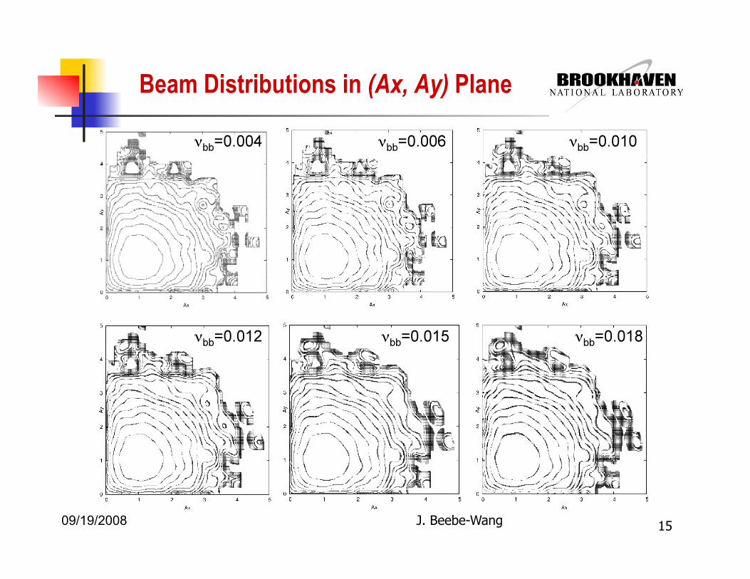
Beam Distributions in (Ax, Ay) Plane

09/19/2008 J. Beebe-Wang 16
RHIC Emittance Measurement

09/19/2008 J. Beebe-Wang 17
Emittance Growth Rate
2 3 4 5 6 7 8 9 10 11 12 13 140
1
2
3
4
5
6
7
8
9
10
11
12
Beam beam Parameter [10 3]
Emitt
ance
Gro
wth
Rat
e [%
per
Hou
r] measurement run 5measurement run 6simulation /sim. line fit /

09/19/2008 J. Beebe-Wang 18
Discussion on Comparison of Simulation to Experiment
The simulation result is slightly higher than the experiment.
Experiment: The measured emittance was averaged over 4 hours of beam store from 1.5 hours to 5.5 hours after the accelaration ramp event (accramp). The beam-beam parameter was measured at the beginning of the 4 hour period (not averaged). Thus, the average value of beam-beam parameter over the 4 hour period could in fact be lower if the effect of beam intensity drop and the beam emittance growth were included.
Simulation: Tracks the initial 2.13 minute after the beams are brought to perfect head on collision, when the intensity drop and emittance blow up are both the strongest. This may account for the higher emittance growth rate predicted by the simulation as compared with the calculation based on ZDC measurements.

09/19/2008 J. Beebe-Wang 19
RHIC RF System Upgrade

09/19/2008 J. Beebe-Wang 20
Emittance Growth vs Bunch Length
Emittance growth rate as function of σRMS from polynomial curve fit: dε/ε = 0.01324 σRMS
3 -0.0727 σRMS2 +0.101σRMS-0.003
20 30 40 50 60 70 80 90 100 1101.21.41.61.8
22.22.42.62.8
33.23.43.63.8
44.24.4
RMS bunch length RMS [cm]
Emitta
nce gro
wth rat
e [% pe
r hour]
Full bunch length Full [nsec]
LIFETRC simulationPolynomial curve fit
3 4 5 6 7 8 9 10 11 12 13 14
1.21.41.61.8
22.22.42.62.8
33.23.43.63.8
44.24.4

09/19/2008 J. Beebe-Wang 21
1. The simulations of RHIC 2006 run and the measurement from ZDC are in reasonably good agreement.
2. Magnet nonlinearities and noises are not included so far. A) Can’t directly tack MAD nonlinear model as input. B) There is a plan to build a more advanced model or, at least, include
the magnet errors in the form of global noise matrix.
3. The cooling effect could be investigated in the form of damping. (Currently looking into related issues)
2. Simulations on emittance growth vs. bunch length gave incoraging result. However, we need more detailed studies with the conditions of proposed RF upgrades. Currently in the prograss of setting up models for simulations with A) 28MHz RF system B) 56MHz RF system C) RF system for 250GeV protons
Conclusion and future work