Becoming oldest-old: evidence from historical U.S. data

GENUS, LXI (No. 1), 125-161

125

DORA L. COSTA – JOANNA LAHEY

Becoming oldest-old: evidence from historical U.S. data 1. INTRODUCTION

The twentieth century has witnessed remarkable declines in older age

mortality in Western Europe, Japan, and the United States (Robine and Vaupel, 2002; Kannisto, 1996; Vaupel, 1997; Wilmoth et al. 2000). The first documented 111 year old died in 1932 and the first verified 122 year old died in 1997 (Vaupel, 1997). Not only has the maximum age of death increased, but the number of people living beyond 100 has increased as well, calling into question whether the upper limit to the length of human life postulated by Fries (1980) is anywhere in sight and whether such an upper limit even exists (Vaupel and Jeune, 1995; Wilmoth and Lundström, 1996). In the United States life expectancy in 1900 at age 65 for both sexes combined was less than 12 years and only 13 percent of all 65 year olds could expect to reach age 85 and join the ranks of the oldest old. By century’s end life expectancy at age 65 had risen to almost 17 years and 42 percent of all 65 year olds could expect to live until age 85. This increase in life expectancy was extremely slow at first, rising by only half a year during the first three decades of the twentieth century. Since 1930 the increase in life expectancy at age 65 has accelerated to 2 years between 1930 and 1960 and then to 3 years between 1960 and 19991.

What accounts for the twentieth century increase in life expectancy and in the proportion of the older population who have become oldest-old? Scientists account for change by genetic evolution, postulating that mutations with bad effects at late ages have bad effects at young ages thus weeding out late-age failures (e.g. Charlesworth, 2001). In contrast, demographers and economists have pointed to the environment. Robine (2003; 2001) argues that contrary to most scientists’ assumptions, the environment, not genetics, determines life span with genetics accounting for individual variation in life spans. Empirically we observe that as individuals age mortality rates increase at a roughly constant rate until around age 109 and then plateau or even decline (Thatcher et al., 1998; Vaupel et al., 1998). Robine (2003) hypothesizes that while the shape of the mortality trajectory

1 See the Berkeley Mortality Database and the Human Mortality DataBase, http://www.mortality.org. All life expectancies are period life expectancies.


126

may be a biological constant, its level, the rate of increase in mortality rates, and perhaps even the age at which the plateau is reached, is determined by the environment. Fogel and Costa (1997) and Fogel (1994) have argued that the unprecedented degree of control that humans have gained over their environment in the last 300 years has led to changes in human physiology that have lengthened life and improved health. Just over the last 100 years major environmental changes in the developed world include the virtual elimination of the infectious diseases that ravaged childhood, the dramatic expansion of the supply of calories and of micro-nutrients, the control of chronic disease conditions through new drugs and surgeries, increased knowledge (though not always application) of good health and dietary habits, and reduced exposure to physical hazards, including environmental pollutants and poisons, both in the home and in the workplace.

If the environment determines life span then such environmental insults as infectious disease, poor nutrition, low socio-economic status, or occupational hazards have a permanent scarring effect, leading to death at later ages by leaving survivors with permanent damage to their hearts, lungs, or other organs as in the case of rheumatic fever or tuberculosis. However, it is not clear a priori that environmental insults necessarily reduce longevity. Individuals who are more frequently exposed to disease may acquire full or partial immunities to such diseases as typhoid or influenza. If only the healthiest survive insults, then selection may lead to a negative relationship between insults and later mortality. Although a large body of research has found evidence that environmental insults, including those in utero and early childhood, affect older age health and longevity (Costa, 2003; Doblhammer and Vaupel, 2001; Preston, Hill and Drevenstedt, 1998; Manton, Stallard and Corder, 1997; Costa, 2000; Elo and Preston, 1992; Barker, 1992, 1994; cf. Christensen et al., 1995; Kannisto, Christensen and Vaupel, 1997; Kannisto, 1994), much of this research can be criticized on the grounds that an observed positive relationship between insults and later death may result from correlation between insults and an omitted variable such as life-long poverty (Paneth and Susser, 1995).

This paper reviews the literature on causes of lengthening life, emphasizing what scholars have learned from studying past populations, and uses historical data to assess the impact of environmental insults in early childhood and at later ages on the mortality of men and women in their sixties and seventies, focusing primarily on the effects of insults related to nutrition and infectious disease. Although we do not present new evidence on the roles of improvements in medical care, changes in health or dietary habits, and reduced exposure to environmental pollutants and poisons in the twentieth century mortality decline, we briefly discuss these factors. We

BECOMING OLDEST -OLD: EVIDENCE FROM HISTORICAL U.S. DATA

127

present new evidence on the effects of immigration on historical United States mortality patterns. Manton and Vaupel (1995) suggest that because immigrants are healthier, recent increases in life expectancy in the United States could arise from immigration. All of our analyses emphasize the predictors of survival to become oldest-old, a rare achievement for most of our ancestors.

The paper first reviews the types of historical data that are available. The next two sections discuss the impact of insults in early childhood and in later life, respectively, on older age mortality. The indicators of environmental stress that we focus on are quarter of birth, residence, socioeconomic status, and the incidence of specific infectious diseases. The fourth section examines the mortality experience of immigrants relative to the native-born in both the nineteenth and the twentieth century. The fifth section evaluates the likely magnitude of environmental insults on older age mortality. The sixth section discusses anthropometric indicators of environmental stress, because these have been widely used in the literature. The seventh section discusses alternative explanations for the mortality decline at older ages. We then summarize our results and conclude with some thoughts on future trends in life expectancy at older ages.

2. HISTORICAL DATA Historical data are useful for establishing long-term mortality trends and

for investigating the determinants of mortality under very different environmental conditions. Past populations were exposed to a wide variety of infectious diseases which varied greatly depending upon size of city of residence. They faced greater nutritional stress both because of their greater poverty and because their intake of vitamins and nutrients was determined by the local agricultural cycle. In addition, they faced high occupational risks and had medical care that was ineffective at best, thus allowing us to examine the effects of untreated infectious disease on later mortality.

Much of the initial work with historical data used aggregate data (e.g. Preston and Van de Walle, 1978; Condran and Cheney, 1982) and these are still valuable in understanding mortality trends at older ages (e.g. Wilmoth and Horiuchi, 1999). However, a disadvantage of aggregate data is that it is very hard to identify the effects of environmental stress on mortality and even harder to distinguish the effects of different types of stresses. Demographers and economic historians have therefore turned to individual-level data.

Individual-level data has consisted of either cross-sectional data with


128

retrospective mortality information or longitudinal data. Cross-sectional data with retrospective mortality information includes the 1900 and 1910 micro-census data with its questions on number of children ever born and number of children surviving used by Preston and Haines (1991) to study the predictors of child mortality. It also includes the 1850 and 1860 census mortality schedules linked to the 1850 and 1860 census population schedules used by Ferrie (2003).

Group level longitudinal data can be created from such individual-level data as the census micro samples. For example, Lleras-Muney (2002) used the 1960-1980 micro census samples to examine the causal effect of education on 10 year mortality, creating cells based upon sex/cohort and state of birth and instrumenting for education with the compulsory school laws that were in effect between 1915-1939. A potential drawback to creating group level artificial cohorts is that for the variables of interest the cell sizes may be too small.

The individual-level longitudinal datasets that have been created have varied widely in the number of years of life that they cover. Steckel (1988) linked households across the 1850 and 1860 censuses to study the mortality of women and children. Preston, Hill and Drevenstedt (1998) linked African-Americans who survived until age 85 to either their 1900 or 1910 household and used these censuses to draw a control sample. Perhaps the most ambitious linkage project of all has been the creation of the dataset, The Aging of Union Army Veterans, available for download from http://www.cpe.uchicago.edu. These data, collected by a team of researchers led by Robert Fogel, cover the life histories of men born between 1820 and 1850, and who reached age 65 between 1885 and 1915. The sample is based upon 35,570 white males who were mustered into the Union Army during 1861-1865. Socioeconomic and biomedical histories of the recruits from childhood to death were created by linking together information from different sources, including military records, pension records, reports from examining surgeons, and the 1850, 1860, 1900, and 1910 censuses.

The new results in this paper are based upon both group-level longitudinal data created from the public use micro census samples and upon individual-level longitudinal data from the Union Army data2.

2 The results presented here for the Union Army data differ from those in Costa (2003) because a larger sample size is used and because the effects of additional variables such as quarter of birth and family income are examined.


129

3. INSULTS IN EARLY CHILDHOOD There is a large body of literature stressing the connection between

intrauterine and infant growth and premature morbidity and mortality at ages above 50. The diseases that are most closely linked to anthropological markers of maternal and intrauterine deprivation are hypertension, coronary heart disease, cerebral hemorrhage, and type II diabetes (Barker, 1992, 1996; Eriksson et al., 2000). Much of the evidence comes from studies carried out by Barker and his collegues in Britain, but there is also evidence from Sweden, Finland, and India (Hyppönen et al., 2001; Leon et al., 1998; Forsén et al., 1999; Stein et al., 1996). These studies have been criticized for not adequately adjusting for such confounding factors as middle -age variations in nutrition and life style and for reflecting the impact of random error (Huxley, Neil and Collins, 2002; Paneth and Susser, 1995; Scrimshaw, 1997). Other studies have found no evidence that intrauterine growth retardation affects later mortality. Christensen et al. (1995) compare twins and singletons and find no mortality differentials except among women age 60-84, among whom twin mortality was higher. Almond, Chay, and Lee (2004) find no evidence that the lighter birth weight twin suffers increased mortality after one year. But, twinning may well be a different process from intrauterine growth retardation. Kannisto, Christensen, and Vaupel (1997) find no evidence of increased mortality in later life for cohorts born dur ing famine compared to cohorts born 5 years before and 5 years after the famine, but variation across cohorts may not be enough to identify the effects of famine if nutritional stress in childhood and of the mother also has an effect on mortality. Steckel (1989) documents that although American slave children experienced such severe deprivation that by four and half years of age they were only at the 0.2 height centile, below the level of the poorest populations of developing countries, they experienced remarkable catch-up growth when they reached field hand age and large quantities of meat were introduced into their diets. By adulthood slaves were only slightly shorter than whites and their mortality rates at ages 20-24 were comparable to those of whites, suggesting to us that while slaves’ early childhood did leave a scarring effect, rapid improvements in conditions during adolescence minimized the scar’s impact.

Some of the strongest evidence for the impact of early life environmental factors on older age mortality comes from studies of the effect of month of birth (Doblhammer and Vaupel, 2001; Doblhammer, 1999; Gavrilov and Gavrilova, 1999). Doblhammer and Vaupel (2001) find that in Austria and Denmark fifty year olds born in the fourth quarter live longer than those born in the second quarter whereas in Austalia the pattern


130

among the native-born is shifted by half a year but among the British-born it is similar to that observed in Austria and Denmark. Kanjanapipatkul (2002) finds that Union Army veterans born in the second quarter experienced shorter life-spans than Union Army veterans born in the fourth quarter. (In contrast, Huntington (1938) found that in a sample of genealogies individuals born in February or March lived longer than those born in July or August.) Doblhammer and Vaupel (2001) reject the hypotheses that season of birth is an indicator of social status or of age and hypothesize that month of birth has an effect on older age mortality through birth weight, pointing out that in Austria during the crisis years of 1916-1922 children born in the fall had higher birth weights than those born in other seasons (Ward, 1993: 22).

Additional evidence for the impact of early life environmental factors on older age mortality comes from historical studies of the impact of place of birth. Preston, Hill, and Drevenstedt (1998) find that among African-Americans farm background was a strong predictor of survival to age 85. Costa (2003) finds that enlisting in a large city (a proxy for growing up in a large city) had a large negative effect on survival among Union Army veterans who lived until age 50 even controlling for size of current city of residence. There is, however, also evidence that under the extreme disease conditions of Union Army camp life growing up in a large city relative to an isolated rural area had a beneficial mortality effect, because men from isolated areas lacked immunities to the diseases that ravaged Union Army camps (Lee, 2003).

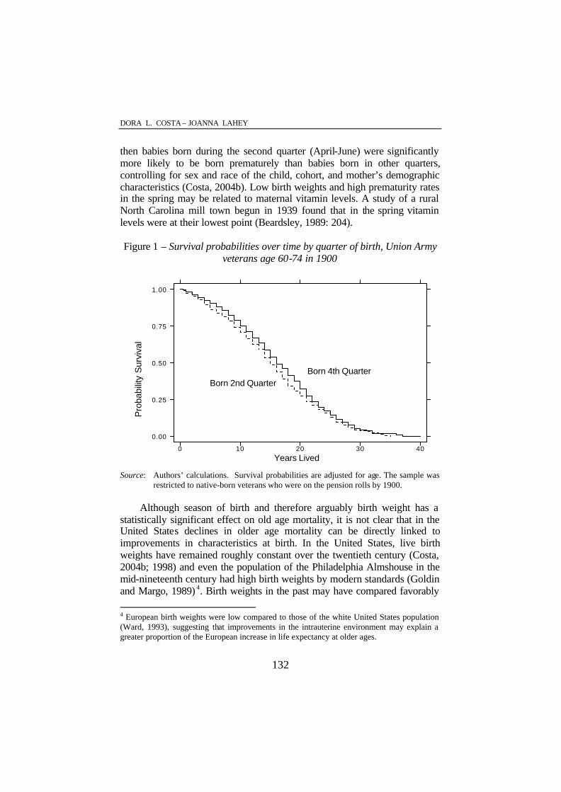
In the United States both quarter and region of birth predict ten year mortality rates of 60-79 year-olds in 1960-1980 (see Table 1). Controlling for age group, sex, and cohort, the ten year mortality rate of men and women born in the Midwest and West was lower by 0.01 and 0.05, respectively, than that of their counterparts born in the Northeast. The ten year mortality rate of men and women born in the second quarter was higher by 0.03 than that of their counterparts born in the fourth quarter, an 8 percent increase in the mean ten year mortality rate of 0.36, and the effect was strongly statistically significant3.

Figures 1 and 2 illustrate the importance of season and of place of birth on the survival probabilities of Union Army veterans who were age 60-74 in 1900. Adjusting for age, veterans born in the second quarter had lower survival probabilities than those born during the fourth quarter. Those born during the first and third quarters also had higher survival probabilities than 3 We did not find differences in the effect of quarter of birth by region. Note that the linear specification provides a better fit. We suspect that this is because we examine a relatively narrow age group.


131

Table 1 – Effects of region and season of birth on ten year mortality rates of 60-79 year-olds in the United States, 1960-1980

Linear specification Log-linear specification Coefficient Std error Coefficient Std error Dummy=1 if born in the Northeast Midwest -0.014 *** 0.006 -0.040 0.038 South -0.005 0.005 -0.006 0.033 West -0.053 *** 0.005 -0.195 *** 0.058 Dummy=1 if born in First quarter 0.003 0.005 0.012 0.043 Second quarter 0.030 *** 0.006 0.118 *** 0.043 Third quarter 0.013 ** 0.006 0.046 0.047 Fourth quarter R2 0.984 0.929 Notes: 128 observations. Each observation is an age group, sex, cohort, region, and quarter

of birth cell. The sample was restricted to the native-born. The dependent variable in the linear specification is the 10 year mortality rate of each cell. The dependent variable in the log-linear specification is the logarithm of the 10 year mortality rate. The mean weighted 10 year mortality rate was 0.36. Additional controls include dummies for age 70 or older, female, and birth cohort (1900-1909 and 1910-1919, with 1890-1899 as the omitted category). The ordinary least squares regression is weighted by cell size. The symbols *** and ** indicate that the coefficient is statistically significantly different from zero at the 1 and 5 percent level, respectively.

Source: Authors’ calculations from the Integrated Public Use Census Samples.

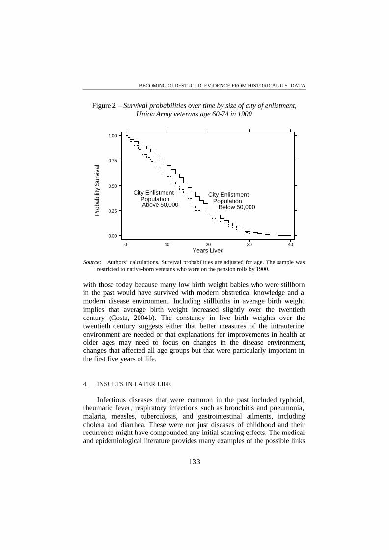
those born during the second quarter (not shown). Veterans who enlisted in a city whose popula tion was above 50,000 in 1860 (the largest 16 cities in the country), faced an elevated mortality risk relative to those who enlisted in smaller cities. Even though food was plentiful and may have been more varied than in rural areas, rising population density and poor sanitation made the largest cities in the country particularly lethal. Life expectancy at birth in the largest Northern cities was only 24. Because city of enlistment was a good indicator of city of birth (Costa 2003), city of enlistment provides a good indication of environmental stress both at birth and in early childhood.

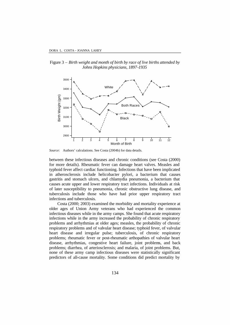
Data on birth weight from Johns Hopkins Hospital provide suggestive evidence that those born during the spring (March-May) fared worse than those born at other times of the year (see Figure 3). Controlling for prematurity, the sex and race of the child, cohort, and mother’s demographic characteristics, babies born in the spring weighed 81 grams less than those born in the summer. For full-term births the difference was 73 grams controlling for gestational age. When season of birth was defined by quarter,


132

then babies born during the second quarter (April-June) were significantly more likely to be born prematurely than babies born in other quarters, controlling for sex and race of the child, cohort, and mother’s demographic characteristics (Costa, 2004b). Low birth weights and high prematurity rates in the spring may be related to maternal vitamin levels. A study of a rural North Carolina mill town begun in 1939 found that in the spring vitamin levels were at their lowest point (Beardsley, 1989: 204).

Figure 1 – Survival probabilities over time by quarter of birth, Union Army

veterans age 60-74 in 1900

P

roba

bilit

y S

urvi

val

Years Lived0 10 20 30 40

0.00

0.25

0.50

0.75

1.00

Born 4th QuarterBorn 2nd Quarter

Source: Authors’ calculations. Survival probabilities are adjusted for age. The sample was

restricted to native-born veterans who were on the pension rolls by 1900. Although season of birth and therefore arguably birth weight has a

statistically significant effect on old age mortality, it is not clear that in the United States declines in older age mortality can be directly linked to improvements in characteristics at birth. In the United States, live birth weights have remained roughly constant over the twentieth century (Costa, 2004b; 1998) and even the population of the Philadelphia Almshouse in the mid-nineteenth century had high birth weights by modern standards (Goldin and Margo, 1989) 4. Birth weights in the past may have compared favorably 4 European birth weights were low compared to those of the white United States population (Ward, 1993), suggesting that improvements in the intrauterine environment may explain a greater proportion of the European increase in life expectancy at older ages.


133

Figure 2 – Survival probabilities over time by size of city of enlistment, Union Army veterans age 60-74 in 1900

P

roba

bilit

y S

urvi

val


0.00

0.25

0.50

0.75

1.00

Above 50,000Population

City Enlistment

Below 50,000Population

City Enlistment


restricted to native-born veterans who were on the pension rolls by 1900.

with those today because many low birth weight babies who were stillborn in the past would have survived with modern obstretical knowledge and a modern disease environment. Including stillbirths in average birth weight implies that average birth weight increased slightly over the twentieth century (Costa, 2004b). The constancy in live birth weights over the twentieth century suggests either that better measures of the intrauterine environment are needed or that explanations for improvements in health at older ages may need to focus on changes in the disease environment, changes that affected all age groups but that were particularly important in the first five years of life.

4. INSULTS IN LATER LIFE Infectious diseases that were common in the past included typhoid,

rheumatic fever, respiratory infections such as bronchitis and pneumonia, malaria, measles, tuberculosis, and gastrointestinal ailments, including cholera and diarrhea. These were not just diseases of childhood and their recurrence might have compounded any initial scarring effects. The medical and epidemiological literature provides many examples of the possible links


134

Figure 3 – Birth weight and month of birth by race of live births attended by Johns Hopkins physicians, 1897-1935

Both Races

White

Birt

h W

eigh

t (gm

)

Month of Birth

Black

1 2 3 4 5 6 7 8 9 10 11 12

2900

3000

3100

3200

3300

3400

3500

Source: Authors’ calculations. See Costa (2004b) for data details.

between these infectious diseases and chronic conditions (see Costa (2000) for more details). Rheumatic fever can damage heart valves. Measles and typhoid fever affect cardiac functioning. Infections that have been implicated in atherosclerosis include helicobacter pylori, a bacterium that causes gastritis and stomach ulcers, and chlamydia pneumonia, a bacterium that causes acute upper and lower respiratory tract infections. Individuals at risk of later susceptibility to pneumonia, chronic obstructive lung disease, and tuberculosis include those who have had prior upper respiratory tract infections and tuberculosis.

Costa (2000; 2003) examined the morbidity and mortality experience at older ages of Union Army veterans who had experienced the common infectious diseases while in the army camps. She found that acute respiratory infections while in the army increased the probability of chronic respiratory problems and arrhythmias at older ages; measles, the probability of chronic respiratory problems and of valvular heart disease; typhoid fever, of valvular heart disease and irregular pulse; tuberculosis, of chronic respiratory problems; rheumatic fever or post-rheumatic arthopathies of valvular heart disease, arrhythmias, congestive heart failure, joint problems, and back problems; diarrhea, of arteriosclerosis; and malaria, of joint problems. But, none of these army camp infectious diseases were statistically significant predictors of all-cause mortality. Some conditions did predict mortality by


135

cause. For example, respiratory infection predicted death from respiratory disease, diarrhea predicted death from gastrointestinal and stomach ailments, and rheumatic fever predicted death from myocarditis. Men who had been prisoners of war and therefore had probably suffered gastrointestinal ailments during their imprisonment, were more likely to die from stomach ailments. Because a large fraction of deaths among Union Army veterans were from infectious, respiratory, and diarrheal disease, it may be difficult to detect the effects of early life and young adult events on all cause mortality because such current events as recent exposure to infectious and parasitic disease may have been more important.

Occupational hazards may also have scarring effects on older age mortality and morbidity. Lung diseases and respiratory symptoms resulting from occupational exposure to dust, fumes, or gases include asthma, chronic bronchitis, chronic air flow limitation, and turberculosis. Workers in mining, steel foundries, tool grinding, glassmaking, metal casting, and stone polishing are particularly prone to occupational lung disease. Farmers are also affected because they inhale organic dust from moldy plant materials and from animal waste, hair, and feathers. Occupational stress is also an important determinant of musculoskeletal capacity. Among Union Army veterans, those in a manual occupation (including farming), disproportionately suffered from arthritis and from back problems at older ages. Veterans who had worked in occupations where they were exposed to dust and fumes were more likely to suffer respiratory ailments at older ages (Costa, 2000). Although laborers were significantly more likely to die of heart disease than farmers, occupation had no effect on the all cause mortality of Union Army veterans (Costa, 2003). Note that in data on more recent populations, occupational differences in all-cause mortality are more pronounced. The most common causes of death may now be those where socioeconomic status has the largest impact. Alternatively, the relationship between socioeconomic status and mortality may have changed. Both United States and British studies from the 1930s and 1940s found a positive correlation between high socioeconomic status and risk of coronary heart disease in men, but studies from 1940 to 1960 found a negative correlation (Manton et al., 1997).

Evidence for the impact of income on mortality in historical United States populations is mixed. Wealth conveyed no systematic advantage for survival of women and children in households matched in the 1850 and 1860 censuses (Steckel, 1998). Preston and Haines (1991) used the questions on number of children ever born and number of children still living in the 1900 census to report that place of residence and race were the most important correlates of child survival in the late nineteenth century, much more


136

important than father’s occupation. Preston and Ewbank (1990) find that infant mortality differentials by social class increased from 1900 to 1930, perhaps because the germ theory of disease first spread to the more educated classes. However, even before knowledge of the germ theory of disease, income enabled individuals to buy lower room congestion, housing in an area of a city with better sanitation, better food, and less work away from home for the pregnant mother. Within U.S. cities there was a steep gradient between infant mortality and family income (e.g. see Rochester (1923)). Chapin (1924) reported that in Providence, Rhode Island, in 1865 the annual crude death rate for taxpayers was 11 per thousand, while the corresponding rate for non-taxpayers was 25 per thousand. Ferrie (2003) linked households in 1850 and 1860 to one year mortality rates as reported in the 1850 and in the 1860 censuses of mortality and found a wealth gradient in rural areas of the United States. Those with greater personal wealth were less likely to die from any cause and were less likely to die from pulmonary tuberculosis, a disease associated with crowding and poor housing. They were not more likely to die of cholera, a disease spread through contaminated water supplies because they did not know how to protect themselves from cholera.

Figures 4 and 5 illustrate the impact of personal property wealth in 1860 and of occupation at enlistment on the age adjusted survival probabilities of Union Army veterans age 60-74 in 1900. Those of higher socioeconomic status were favored in survival. These measures of socioeconomic status will be strongly correlated with the socioeconomic status of the household veterans grew up in as children (if they had not yet formed their own households then wealth is parental family wealth) and will also be correlated with socioeconomic status later in life. Although we cannot adjust for wealth later in the life-cycle, when we adjust for occupational class at older ages we find that occupation at enlistment still has an effect on older age mortality.

The graphs of survival probabilities over time of Union Army veterans show that the effects of such environmental factors as quarter of birth, city of enlistment, wealth, and occupation diminish with age. They also suggest that at very late ages, survival probabilities no longer fall as steeply as at younger ages.

5. IMMIGRATION Recent increases in life expectancy in the United States may arise from

increased migration. Manton and Vaupel (1995) suggest that immigrants are healthier than the people who did not choose to immigrate, and probably have healthier children as a result. Nineteenth century migration, however,


137

Figure 4 – Survival probabilities over time by personal property wealth in 1860 family, Union Army veterans age 60-74 in 1900

P

roba

bilit

y S

urvi

val


0.00

0.25

0.50

0.75

1.00

Low Wealth

High Wealth

Source: Authors’ calculations. High Wealth is defined as holdings of $250 or more. Survival

probabilities are adjusted for age. The sample was restricted to native-born veterans who were on the pension rolls by 1900.

may have been harmful to health. European soldiers were long aware that strange “climates’’ could have fatal effects (Curtin, 1989). Large cities, and particularly their immigrant wards, were the sources of many epidemics. Sánchez (2003) used the longitudinal residential information in the Union Army records to trace the effects of internal migration on life expectancy. He found that migrants were more likely to die of infectious disease than non-migrants and that although mortality rates were higher among migrants to urban areas than among migrants to rural areas, even migrants to rural areas faced an elevated mortality risk compared to non-migrants.

Table 2 shows the impact of foreign-birth on the ten year mortality rate of white 60-79 year olds differs by cohort. There was no statistically significant difference in mortality rates at older ages between immigrants and the native-born among cohorts born 1830-1859. But, among cohorts born 1870-1899, the foreign-born faced a higher mortality risk at older ages and among cohorts born 1900-1929 the foreign born faced a lower mortality risk at older ages than the native-born. When we examined birth place of origin we found that for the 1830-59 and 1870-99 cohorts the Irish faced higher mortality risk than the Germans or the English and that this risk was


138

Figure 5 – Survival probabilities over time by occupation at enlistment, Union Army veterans age 60-74 in 1900

P

roba

bilit

y S

urvi

val


0.00

0.25

0.50

0.75

1.00

Professional/Proprietor

Laborer


restricted to native-born veterans who were on the pension rolls by 1900.

much higher for the earlier Irish cohort (which had greater life-long poverty and which was born during the Potato Famine) than the later one. For the 1900-29 cohort those born in Mexico and, to a lesser extent, those born in Mediterranean countries faced a lower mortality risk perhaps because immigration from these countries was temporary and those in need of family support returned home.

6. ACCOUNTING FOR MORTALITY IMPROVEMENTS Regression analysis allows us to assess the relative importance of

different types of environmental stress over the life cycle among Union Army veterans age 60-74 in 1900. We model the probability of survival to age 85 by means of a probit equation,

)()()1( ββε XXprobIprob ′Φ=′<== [1]

where 1=I if the veteran survived until age 85, ()Φ is a standard normal cumulative distribution function, and X is a vector of control variables. The


139

TABLE 2 PAGE 1 OF 1


140

effect of a unit change in one of the independent variables on the probability of having a given chronic condition is given by the partial derivative of the probit function P with respect to that independent variable. We model the number of years lived after 1900 by means of a hazard model, in which our estimated hazard, ),(tλ is

,)()exp()( 0 tXt λβλ ′= [2]

where X is the vector of control variables and )(tOλ is the baseline hazard which we assume to be Gompertz, )exp()( ttO γλ = 5. The hazard ratios that we report indicate whether a one unit change in an independent variable gives an increase/decrease in the odds of an event. For the sample of men for whom cause of death is known, we estimate separate independent competing risk models for five specific causes of death, treating other causes of death as censored. The five specific causes of death that we examine are death from heart disease (excluding stroke), death from stroke, death from infectious diseases (including tuberculosis), death from both chronic and acute respiratory ailments such as pneumonia, influenza, and acute bronchitis, and death from stomach ailments such as gastritis/duodentitis and ulcers. Our estimated hazard, )(tiλ , for one of our five models (i), is

,)()exp()( 0 tXt iii λβλ ′= [3]

where X is the vector of control variables and )(tiOλ is the baseline hazard which we assume to be Gompertz.

The primary control variables used in the analysis are season of birth (four quarters); size of city of enlistment (50,000 and over, 25,000-50,000, 2500-25,000, and less than 2500); a dummy equal to one if the household’s total personal property wealth in 1860 was greater than $250; occupation at enlistment and occupation circa 1900, using last known occupation for the

5 A Gompertz model is favored over a Weibull or log-logistic model by the Aikaike information criterion, but using these other models yields very similar conclusions. Using the Gompertz model we cannot reject the hypothesis that there is unobserved individual level heterogeneity whereas we can reject this hypothesis using the other models, suggesting that we should be using a model in which after a while individual hazards fall. However, the estimated heterogeneity parameter is quantitatively small and the parameter estimates remain very similar, perhaps because relatively few individuals survive to ages where individual hazards begin to fall. (Parametric estimates suggest that the hazard does not fall until after age 99, when only 1 percent of the sample was alive.) For simplicity we therefore present the Gompertz models.


141

retired (farmer, professional, manager or proprietor, clerical service, craft, operative, service, and laborer); prisoner of war status; and infectious disease experienced while in the service (diarrhea, respiratory, measles, tuberculosis, rheumatism/rheumatic fever, malaria, typhoid, stomach ailments, and syphilis). Additional control variables include age in 1900, indicators of missing information, a dummy indicating whether the veteran was ever wounded in the war, size of city of residence in 1900, and marital status in 1900.

Being born in the second relative to the fourth quarter decreased the probability of survival to age 85 by 0.04, a decline of 23 percent relative to the predicted sample survival probability of 0.17 (see Table 3) 6. Enlisting in a large rather than a small city had a larger effect on the probability of survival to age 85, lowering the probability of survival to age 85 by 0.06. Relative to men who were farmers at enlistment, men who were laborers had a survival probability that was lower by 0.05. Occupation circa 1900 and wartime service had no effect on the probability of surviving until age 85. Although enlisting in a large city had the largest effects on mortality, relatively few men in enlisted in a large city. If no one had enlisted in a large city the predicted probability of survival would have been 0.18. In contrast if no one had been born in the second quarter the predicted probability of survival would have been 0.19. If everyone had been a farmer at enlistment the predicted probability of survival would have been 0.19 and if everyone had been a professional the predicted probability would have been 0.21.

The all-cause mortality hazard model also emphasizes the importance of size of city of enlistment. Enlisting in a large city increased the odds of dying by 1.24. Being born in both the second and third quarter relative to the fourth quarter increased the odds of dying by 1.10. Non-farmers faced an elevated mortality risk. Although being an operative at enlistment rather than a farmer increased the odds of dying by 2.02, a large standard error means that the effect was not statistically significant. Those with high personal property wealth faced a lower odds of death. Using the hazard model specification, the largest effects on mortality come from high personal property wealth. If everyone had had high personal property wealth then the predicted median number of years lived after 1900 would have been 12.8,

6 The probability of survival in this sample is higher than that from a 1900 life table for the death registration states. In the 1900 life table men age 65 (the mean age in the Union Army sample) had only a 13 percent chance of surviving to age 85 and a life expectancy of 11.4 years. In contrast life expectancy among Union Army veterans was 12.6. Mortality rates life table for the death registration states probably overstate the national average because the death registration states were disproportionately the urban, Northeastern states in which mortality was higher.


142

Table 3 – Probability model of surviving to age 85 and hazard model of years to death, Union Army veteran age 60-74 in 1900

Probit model Hazard model dP/dx Std error Hazard rate Std error Dummy=1 if born

First quarter -0.012 0.016 1.062 0.048 Second quarter -0.036 ** 0.016 1.105 ** 0.051 Third quarter -0.014 0.017 1.095 ** 0.051 Fourth quarter

Dummy=1 if enlisted in city with population of 50,000+ -0.055 * 0.027 1.241 *** 0.102 25,000-50,000 -0.028 0.032 1.063 0.096 2,500-25,000 -0.016 0.013 1.056 0.036 Less than 2,500

Dummy=1 if personal property wealth in 1860 household above $250 0.023 0.016 0.925 * 0.039

Dummy=1 if occupation at enlistment Farmer Professional 0.022 0.038 1.024 0.097 Manager/Proprietor -0.100 * 0.044 1.183 0.211 Clerical/Service -0.008 * 0.053 1.073 0.157 Craft -0.034 0.018 1.130 ** 0.057 Service 1.118 * 0.076 Operative -0.050 ** 0.022 2.022 0.836 Laborer -0.014 0.021 1.074 0.062

Dummy=1 if occupation circa 1900 Farmer Professional -0.001 0.034 1.079 0.098 Manager/Proprietor 0.008 0.026 0.976 0.067 Clerical/Service 0.001 0.034 0.956 0.087 Craft -0.003 0.020 1.009 0.054 Operative -0.024 0.024 1.208 ** 0.082 Service -0.009 0.048 1.144 0.146 Laborer -0.001 0.019 1.066 0.055

Dummy=1 if was POW -0.020 0.019 1.046 0.055 Dummy=1 in service had

Diarrhea -0.002 0.012 1.017 0.034 Respiratory -0.020 0.016 1.065 0.047 Measles 0.016 0.027 0.903 0.063 Tuberculosis 0.022 0.043 0.900 0.096 Rheumatism/rheumatic fever -0.022 0.016 1.033 0.045

Observations 4,641 4,647 Pseudo R2 0.030 ? 0.090 *** 0.002 ?2(42) for significance of all coefficients 481.770 0.000


143

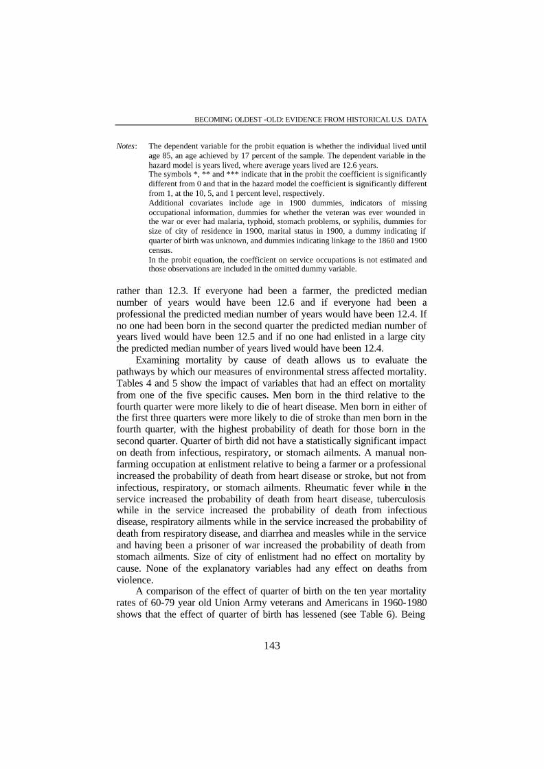
Notes: The dependent variable for the probit equation is whether the individual lived until age 85, an age achieved by 17 percent of the sample. The dependent variable in the hazard model is years lived, where average years lived are 12.6 years. The symbols *, ** and *** indicate that in the probit the coefficient is significantly different from 0 and that in the hazard model the coefficient is significantly different from 1, at the 10, 5, and 1 percent level, respectively. Additional covariates include age in 1900 dummies, indicators of missing occupational information, dummies for whether the veteran was ever wounded in the war or ever had malaria, typhoid, stomach problems, or syphilis, dummies for size of city of residence in 1900, marital status in 1900, a dummy indicating if quarter of birth was unknown, and dummies indicating linkage to the 1860 and 1900 census. In the probit equation, the coefficient on service occupations is not estimated and those observations are included in the omitted dummy variable.

rather than 12.3. If everyone had been a farmer, the predicted median number of years would have been 12.6 and if everyone had been a professional the predicted median number of years would have been 12.4. If no one had been born in the second quarter the predicted median number of years lived would have been 12.5 and if no one had enlisted in a large city the predicted median number of years lived would have been 12.4.

Examining mortality by cause of death allows us to evaluate the pathways by which our measures of environmental stress affected mortality. Tables 4 and 5 show the impact of variables that had an effect on mortality from one of the five specific causes. Men born in the third relative to the fourth quarter were more likely to die of heart disease. Men born in either of the first three quarters were more likely to die of stroke than men born in the fourth quarter, with the highest probability of death for those born in the second quarter. Quarter of birth did not have a statistically significant impact on death from infectious, respiratory, or stomach ailments. A manual non-farming occupation at enlistment relative to being a farmer or a professional increased the probability of death from heart disease or stroke, but not from infectious, respiratory, or stomach ailments. Rheumatic fever while in the service increased the probability of death from heart disease, tuberculosis while in the service increased the probability of death from infectious disease, respiratory ailments while in the service increased the probability of death from respiratory disease, and diarrhea and measles while in the service and having been a prisoner of war increased the probability of death from stomach ailments. Size of city of enlistment had no effect on mortality by cause. None of the explanatory variables had any effect on deaths from violence.

A comparison of the effect of quarter of birth on the ten year mortality rates of 60-79 year old Union Army veterans and Americans in 1960-1980 shows that the effect of quarter of birth has lessened (see Table 6). Being


144

Table 4 – Independent competing risk model of years until death from heart disease (excluding stroke) and from stroke,

Union Army veterans age 60-74 in 1900

Heart disease Stroke Hazard rate Std error Hazard rate Std error Dummy=1 if born

First quarter 0.964 0.121 1.583 ** 0.336 Second quarter 1.141 0.139 1.701 *** 0.362 Third quarter 1.251 * 0.156 1.596 ** 0.347 Fourth quarter

Dummy=1 if occupation circa 1900 Farmer Professional 1.187 0.274 1.174 0.495 Manager/Proprietor 1.146 0.217 1.510 0.430 Clerical/Service 1.442 * 0.294 1.172 0.407 Craft 1.319 ** 0.183 1.429 0.325 Operative 1.324 * 0.225 1.658 * 0.440 Service 1.472 0.407 1.921 0.788 Laborer 1.392 *** 0.185 1.051 0.245

Dummy=1 in service had Rheumatism/rheumatic fever 1.249 ** 0.133 0.778 0.161

Observations 2,178 2,178 ? 0.081 *** 0.005 0.106 *** 0.008 ?2(42) for significance of all coefficients

84.760

0.000

62.780

0.021

Notes: The dependent variables are years lived until death from the specific causes. The symbols *, ** and *** indicate that the coefficient is significantly different from 1 at the 10, 5, and 1 percent level, respectively. Additional covariates include dummies for size of city of enlistment, a dummy for personal property wealth in 1860, dummies for occupation at enlistment, a dummy if the veteran was a POW, dummies if the veteran, while in the service, had diarrhea, respiratory conditions, measles, or tuberculosis, age in 1900 dummies, indicators of missing occupational information, dummies for whether the veteran was ever wounded in the war or ever had malaria, typhoid, stomach problems, or syphilis, dummies for size of city of residence in 1900, marital status in 1900, a dummy indicating if quarter of birth was unknown, and dummies indicating linkage to the 1860 and 1900 census.

born in either the second or third rather than the fourth quarter increased Union Army veterans’ probability of dying by 0.04, a 9 percent increase in the mean ten year mortality rate of 0.45. In contrast, in 1960-1980, using the better fitting linear specification, being born in the second rather than the fourth quarter increased the mean ten year mortality rate of 0.36 by 0.03, an 8 percent increase, and being born in the third rather than the fourth quarter


145

TABLE 5 PAGE 1 OF 1


146

increased the ten year mortality rate by 0.01, a 4 percent increase. Using the log-linear specification reveals an increase in second relative to fourth quarter mortality and a large decrease in third relative to fourth quarter mortality. The declining impact of being born in the summer, a time when the disease burden from water-borne diseases was especially high, suggests improvements in either the intrauterine or the early infancy environment7.

The declining impact of season of birth accounts for roughly 16 to 17 percent of the 0.087 difference in the ten year mortality rates of Union Army veterans and of Americans in 1960-1980. Differences in the seasonality of births in the two samples are negligible 8. Assuming that ten year mortality rates in the Union Army sample and the recent sample can be written as linear functions of quarter of birth using the coefficients in Table 6, the difference in ten year mortality rates due to changes in the coefficients on birth weights can be written as

)(3)(2)(1 ,3,3,2,2,1,1 RqUAqUARqUAqUARqUAqUA qqq ββββββ −+−+−

using the recent function and as

)(3)(2)(1 ,3,3,2,2,1,1 RqUAqRRqUAqRRqUAqR qqq ββββββ −+−+− using the Union Army function, where 1q , 2q , and 3q indicate the first, second, and third quarters and where the subscripts UA and R indicate the Union Army sample and the recent sample, respectively. Using the linear specification, these respective sums yield 0.014 and 0.015, which represents 16 and 17 percent of the difference in ten year mortality rates. The difference in ten year mortality rates due to changes in season of birth is virtually zero.

Rising wealth, an improving disease environment, declining occupational risks, and a more favorable intrauterine environment may explain at least one-fifth of the increase between 1900 and 1999 in the proportion of the population living to age 85 and of the increase in life expectancy at age 65. Between 1900 and 1999, the probability that a 65 year old man (the mean age in the Union Army sample) would survive to age 85 rose from 13 to 35 percent and life expectancy at age 65 rose from 11.4 to

7 Kanjanapipatkul (2002) finds that in recent United States data the seasonal pattern differs from that observed at Johns Hopkins and that since the 1960s seasonal fluctations in birth weight have diminished. 8 The fractions born in the first, second, third, and fourth quarters were 0.261, 0.252, 0.241, and 0.245, respectively, in the Union Army sample. The respective fractions for Americans in 1960-1980 were 0.266, 0.232, 0.257, and 0.245.


147

TABLE 6 PAGE 1 OF 1


148

13.5 years9. Had all men in the Union Army sample had a very favorable experience, here proxied as the same mortality experience as men who were farmers at enlistment, who grew up in a small city, who were born in the fourth quarter, and who had high personal property wealth, their predicted probability of living until age 85 would have been 22 percent and their predicted median number of years lived after 1900 would have been 13.5 years instead of the observed probability of living until age 85 of 17 percent and the median number of years lived after 1900 of 12.3. By modern standards this is not a very favorable experience, but over three-quarters of Union Army veterans fared much worse in terms of mortality. The increase of 0.05 in the predicted probability of living to age 85 and the increase of 1.2 years in predicted median number of years lived represents roughly one-fifth of the observed increase in the period life tables. Much of the increase in survival probabilities, however, cannot be explained by our regression models, perhaps because many risks are not observed, but also because, as noted for quarter of birth, the relationship between risk factors and mortality has changed.

7. ANTHROPOMETRIC MEASURES Anthropometric measures provide useful proxies for environmental

stress. Heights have been widely used as proxies for the environmental stress faced by past populations because they were commonly recorded by the military for identification purposes. Additional anthropometric measures that have been used include Body Mass Index (BMI) and measures of central body fat. Poor net nutritional status during the growing years (including the fetal stage) leads to a shorter population and poor current net nutritional status to a lighter population. Low birth weight for gestational age babies not only grow up to be shorter, but they may also grow up to have greater abdominal fat deposits, controlling for body mass (Paz et al., 1993; Lagerström et al., 1994).

Height, weight, and fat patterning are predictors of subsequent morbidity and mortality. Costa (1993) and Costa and Steckel (1997) found that the relationship between height and BMI and subsequent mortality was similar among a sample of Union Army veterans and among modern Norwegians males. All-cause mortality first declines with height to reach a

9 See the Berkeley Mortality Database and the Human Mortality DataBase, http://www.mortality.org. All life expectancies are period life expectancies.


149

minimum at heights close to 185cm and then starts to rise10. All-cause mortality risk first declines at low weights as BMI increases, stays rela tively flat over BMI levels from the low to high twenties, then starts to rise again, but less steeply than at very low BMIs. In recent data low BMIs are associated with respiratory disease and high BMIs with heart disease. Height appears to be inversely related to heart and respiratory disease and positively related to the hormonal cancers (Barker, 1992). It is also related to stroke (McCarron et al., 2001). Abdominal fat distribution is associated with antecedents of cardiovascular disease such as hypertension, non-insulin dependent diabetes, high plasma concentrations of atherogenic lipids, and low concentrations of high density lipoprotein cholesterol (Ohlson et al., 1985; Blair et al., 1984; Folsom et al., 1989). A 23-year follow-up study of WWII soldiers measured prior to discharge in 1946-47 shows that a standard deviation increase in waist-hip ratio above the mean increased mortality risk from ischemic and cerebrovascular heart disease by up to 1.24 times and that this relationship was linear (Terry et al., 1992). Yao et al. (1991) find that measures of central body are linearly related to cardiovascular disease, but, like BMI, they have a U-shaped relation with all cause mortality. Costa (2004a) found that in a sample of Civil War soldiers measured by the United States Sanitary Commission, waist-hip ratio at young adult ages was an excellent predictor of older age mortality from ischemic heart disease or stroke and that the relationship was U-shaped.

In the sample of Union Army veterans used in this paper, height at enlistment was not a predictor of older age mortality. BMI in 1900 was a U-shaped predictor of both all-cause and respiratory disease mortality, but did not significantly affect death from the other specific causes, suggesting that BMI at older ages may be reflecting current underlying disease conditions, particularly respiratory ones. Controlling for all other early and later life socioeconomic and demographic characteristics, men with a BMI of 24 circa 1900 were the most likely to survive to age 85.

Past populations were shorter, lighter, and, controlling for BMI, had more abdominal fat (Fogel and Costa, 1997; Costa and Steckel, 1997; Costa, 2004a). How did changes in frame size affect mortality trends? Costa (1993) calculated that increases in BMI from 1900 to 1986 explain roughly 20 percent of the total decline in mortality above age 50. Costa (2004a) estimated that changes in frame size (height, BMI, and waist-hip ratio) accounted for almost half of the mortality declines among 56-72 year old white men between 1914 and 1988. The impact of changes in frame size on 10 However, in later work Costa (2003) did not find a relationship between height and older age mortality among Union Army veterans. Costa (1993) showed that the relationship between height and mortality among Norwegian males was very sensitive to sample size.


150

mortality may have been even larger in other countries. Changes in French height and weight jointly explain about 90 percent of the decline in French mortality rates between 1785 and 1870 and about half of the decline in the twentieth century, with much of the mortality improvement prior to 1870 due to increases in height and much of it after 1870 due to increases in weight (Fogel and Costa, 1997). These calculations reinforce the importance of environmental stress (though improvements in BMI could arise from better medical control of chronic conditions), but suggest that the childhood factors proxied by height have become less important over time.

8. OTHER FACTORS We estimated that at least one-fifth of the increase between 1900 and

1999 in the probability of a 65 year old surviving to age 85 to become oldest-old may be attributable to improvements in early life conditions. What might account for the remaining four-fifths? Potential explanations include improvements in medical care and knowledge, a move away from salt as a food preservative with the rise of refrigeration, and declines in environmental pollution and poison, among other factors, and these are the explanations that we review below in greater detail. (Other explanations such as smoking may explain the recent decline in death rates, but probably initially increased death rates during the twentieth century.)

Inadequate medical care, such as lack of treatment for heart attacks, can have immediate effects on mortality. Suggestive evidence for the impact of medical care on mortality comes from cross-country mortality comparisons. Velkova, Volleswinkel-Van den Bosch, and Mackenbach (1997) report that temporary life expectancy from birth to age 75 (the average number of years a cohort of newly born infants would live between birth and age 75) was higher by 1.25 to 6.29 years for men and 1.09 to 3.44 years for women in Western compared to Central and Eastern Europe. Excluding neonatal deaths, mortality from conditions amenable to medical intervention accounted for 11 to 50 percent of the difference in temporary life expectancy among men and 24 to 59 percent of the difference among women. Gjonça, Brockman, and Maier (2000) report that among those older than 79 mortality in Western Germany was decreasing since the 1970s whereas in East Germany mortality did not decline until the late 1980s and the decline accelerated sharply after German re-unification when the Western health care and pension system was installed in East Germany and when purchases of fresh fruits and vegetables increased. Bailey and Garber (1997) point out that the United States devotes more resources to curing lung cancer, breast


151

cancer, and diabetes than the United Kingdom and has the more favorable outcomes for breast and lung cancer whereas the United Kingdom has the most favorable outcomes for diabetes, a condition controlled by patient behavior not by capital intensive equipment.

Evidence for the effects of medical care on mortality also come from clinical studies of specific conditions. Cutler, McClellan, and Newhouse (1999) document the substantial change in heart attack treatment from the mid-1970s to the mid-1990s and, based upon their review of clinical studies, conclude that changes in medical treatment used in the management of acute myocardial infarction account for approximately 55 percent of the reduction in mortality that has occurred in acute myocardial infarction cases between 1975 and 1995, a time period when heart attack mortality fell by almost one-third. Their analysis of Medicare claims data from 1984 to 1991 confirms that mortality rates following a heart attack have fallen sharply (by 2 percentage points during the initial hospital stay and by 5 percentage points after one year) and have fallen more for heart attack patients than for the general population of the same age, suggesting that improved medical treatment is the most likely explanation.

The shift from salting and smoking to preserve foods to refrigeration has been pointed to as an explanation for the decline in stroke mortality11. Thus in Belgium where only 21 percent of households had a refrigerator in 1960 compared to 96 percent in the United States (Lebergott, 1993: 111), researchers documented a 50 percent decline in mean 24-hour sodium excretion in subjects studied between 1966 and 1979 (e.g. Joossens, Kesteloot, and Amery, 1979). But, a comparison of age-adjusted international stroke mortality trends (see de Looper and Bhatia (1998)) reveals no clear pattern by refrigerator diffusion. In the United States 44 percent of homes had a refrigerator in 1940, a level achieved in France only 20 years later (Lebergott, 1993: 111, 113), but declines in stroke mortality for men and women were of a similar order of magnitude (around 70 percent) in the two countries between 1950-54 and 1992. Cummins (1983) found that although salt purchases in England and Wales declined between 1958 and 1978, coincident with declines in stroke mortality, the picture is confused by an increase in meals eaten outside the home and by the consumption of more processed foods. Other scholars have questioned whether there even is a relationship between the sodium contents of food and salt use and hypertension (e.g. Harlan et al., 1984). Lawlor et al. (2002) used data on British autopsies to infer that although both cerebral infarct mortality

11 It has also been pointed to as an explanation for declines in stomach cancer because of the interaction between salt and helicobactor pylori (Manton, Stallard, and Corder, 1997).


152

and cerebral hemorrhage mortality have fallen since 1932, the different patterns suggest that the aetiological factors differ. Estimated cerebral infarct mortality first rose and then declined sharply after the 1960s, following a pattern similar to that of coronary heart disease mortality. In contrast, estimated cerebral hemorrhage mortality declined steadily. They hypothesize that whereas smoking and cholesterol may be important risk factors for coronary heart disease and cerebral infarct, early life risk factors may be more important for cerebral hemorrhage12.

Rising urbanization and industrialization, signalled by the heavy black clouds that hung over many early twentieth century cities (Stradling, 1999), may have initially contributed to an upsurge in the United States in respiratory disease and mortality, which then declined with anti-smoke and anti-pollution efforts after World War II. Studies based upon both geographic and temporal variation in air pollution find substantial effects of pollution on mortality and health. Ransom and Pope (1995) measured the external health costs of air pollution by using variation in the operation of a steel mill in a mountain valley in Central Utah and by using a nearby valley as a control. They reported that elevated pollution levels were associated with significant declines in childrens’ lung function and that deaths in Utah county when the steel mill was operating were 3.2 percent higher per day than when it was not. Chay and Greenstone (2003) used geographic variation in the effects of the 1981-1982 recession to find that pollution significantly affects infant deaths, particularly within one month and one day of birth, suggesting that fetal exposure may be harmful. They also find that the incidence of low birth weight babies (less than 2500 grams) falls with declines in pollution.

Another environmental hazard at the beginning of the twentieth century was lead poisoning, which by impairing the immune system, could have far reaching effects on older age mortality (e.g. see Fischbein et al. (1993)). Troesken (2003) documents that in 1897 half of United States municipalities were using water from lead pipes and that lead levels in Massachusetts towns ranged from 3 to 411 times current Environmental Protection Agency guidelines. He finds that the use of lead pipes increased infant mortality rates by 25 to 50 percent, depending on the age of the lead pipes and on the corrosiveness of the water supply. Corrosiveness of the water supply was a problem particularly in New England. Troesken (2003) estimates that between 1910 and 1921, the decline in lead levels in New Hampshire water either from the gradual oxidization of lead pipes and their replacement or

12 Birth weight is strongly inversely associated with cerebral hemorrhage but not with cerebral infarct (Hyppönen et al., 2001; Eriksson et al., 2000).


153

from declining industrial pollution cut infant deaths rates by up 16 percent. Given that roughly 28 percent of all births in the death registration areas were from New England, we calculate that if all of New England experienced New Hampshire’s decline in lead levels then 12 percent of the decline in infant mortality between 1910 and 1921 is explained by reductions in lead levels.

9. CONCLUSION This paper has used longitudinal data on past populations who faced

extreme variations in local environmental conditions to study the role of environmental stress throughout the life cycle on older-age mortality. We found that environmental insults in early childhood and during young adulthood reduced life expectancy. Among Union Army veterans age 60-74 in 1900, those born in either the second or third quarter relative to the fourth, those enlisting in a large city, and those of low socioeconomic status in their youth whether measured by occupation at enlistment or family wealth before the war did not live as long and were less likely to become the oldest-old. The infectious disease that soldiers had while in the army affected their later probability of death from a specific cause. Those who had had rheumatic fever as young men in the army were more likely to die of heart disease after age 60, those who had had tuberculosis were more likely to die of infectious disease, those who had had a respiratory disease were more likely to die of a respiratory disease, and those who had had diarrhea or had been prisoners of war were more likely to die of stomach ailments.

Among Americans in their sixties and seventies in 1960-1980, mortality rates also varied by place of birth and mortality rates were higher for those born in the second and third quarters relative to the fourth quarter, but the magnitude of the effect of quarter of birth, particularly for the third quarter, was smaller in these more recent data than among Union Army veterans. We showed that in the first third of the twentieth century, the birth weights of children born in the spring were lower than those of children born in the summer, suggesting that quarter of birth may in part proxy for intrauterine growth retardation, though it could also reflect seasonal differences in the disease environment a child was born into. We calculated that 16 to 17 percent of the difference in older age ten year mortality rates between Union Army veterans and Americans in 1960-1980 was attributable to the declining impact of quarter of birth on mortality rates. We also estimated that at least one-fifth of the increase between 1900 and 1999 in the probability of a 65 year old surviving to age 85 may be attributable to early life conditions.


154

What explains improvements in early life conditions? The twentieth century witnessed the filtration and chlorination of water, the construction of integrated sewage systems and the adoption of sewage treatment, the cleaning of the milk supply and the eradication of bovine tuberculosis, widespread vaccination against childhood diseases, improved commercial food processing and the supplementation of foods with iodine and iron, the decline in exposure to environmental pollution and poisons both in the home and in the workplace, the decrease in crowding that coincided with reductions in fertility and immigration and with rising incomes, and the availability of more varied and fresher food with the growing use of refrigeration in transportion, in stores, and in the home. The relative contributions of public health campaigns, technological change, and rising wealth to the improvement in early life conditions still remains an issue for future research.

Our findings have implications for future mortality trends. The cohort which will reach age 65 in 2020 was born in 1955 after the steep plunge in infant and child mortality and the historical record suggests that this cohort may be particularly long-lived compared to past cohorts. However, mortality rates may not fall as steeply for the cohorts born after 1955 as for earlier cohorts. The difference in early life conditions for cohorts born in 1955 instead of 1995 was not as stark as that for cohorts born in 1915 instead of 1955. For cohorts born after 1955 improvements in older age mortality rates will need to come from medical care or better health habits and unless the rate of innovation in medical increases the rate of reduction in future mortality improvements may not be as sharp as it has been in the recent past. But, if mortality rates reach a plateau at older ages then as long as we can change the level of the plateau, investments in health at very old ages will not hit diminishing returns.

Acknowledgements Prepared for 2003 IUSSP seminar on “Increasing Longevity: Causes,

Consequences, and Prospects.’’ We thank participants at the NBER Aging Summer Institute, the IUSSP seminar, and the Harvard Economic History Tea for comments. Dora Costa gratefully acknowledges the support of NIH grants R01 AG19637 and P01 AG10120, of the Robert Wood Johnson Foundation, and of the Center for Retirement Research at Boston College pursuant to a grant from the United States Social Security Administration funded as part of the Retirement Research Consortium. The opinions and


155

conclusions are solely those of the authors and should not be construed as representing the opinions or policy of the Robert Wood Johnson Foundation, the National Institutes of Health, the Social Security Administration, or any agency of the federal government, or the Center for Retirement Research at Boston College.

References

ALMOND D., CHAY K.Y., LEE D.S. (2004), The costs of low birth weight, National Bureau of Economic Research Working Paper No. 105502.

BAILY M.N., GARBER A.M . (1997), “Health care productivity”, Brookings Papers on Economic Activity, Microeconomics, 143-202.

BARKER D.J.P. (1992), Fetal and Infant Origins of Adult Disease, London, British Medical Journal Publishing Group.

BARKER D.J.P. (1994), Mothers, Babies, and Disease in Later Life, London, British Medical Journal Publishing Group.

BEARDSLEY E.H. (1987), A History of Neglect: Health Care for Blacks and Mill Workers in the Twentieth Century South, Knoxville, TN, University of Tennessee Press.

BLAIR D., HABICHT J.P., SIMS E.A.H., SYLWESTER D., ABRAHAM S. (1984), “Evidence for an increased risk of hypertension with centrally located body fat and the effect of race and sex on this risk”, American Journal of Epidemiology, 119(4), 526-540.

CHAPIN C.V. (1924), “Death Among taxpayers and non-taxpayers, income tax, Providence, 1865”, American Journal of Public Health, 14, 647.

CHARLESWORTH B. (2001), “Patterns of age-specific means and genetic variances of mortality rates predicted by the mutation-accumulating theory of ageing”, Journal of Theoretical Biology, 210(1), 47-65.

CHAY K.Y., GREENSTONE M. (2003), “The impact of air pollution on infant mortality: Evidence from geographic variation in pollution shocks induced by a recession”, Quarterly Journal of Economics, 118(3), 1121-1167.

CHRISTENSEN K., VAUPEL J.W., HOLM H.V., YASHIN A.I. (1995), “Mortality among twins age 6: Fetal origins hypothesis versus twin method”, British Medical Journal, 310(6977), 432-436.

CONDRAN G., CHENEY R.A. (1982), “Mortality trends in Philadelphia: Age-and case-specific death rates 1870-1930”, Demography, 19(1), 97-123.


156

COSTA D.L. (2004a), “The measure of man and older age mortality: Evidence from the Gould sample”, Journal of Economic History, 64(1), 1-23.

COSTA D.L. (2004b), “Race and pregnancy outcomes in the twentieth century: A long-term comparison”, Journal of Economic History, 64(4), 1056-1086.

COSTA D.L. (2003), “Understanding mid-life and older age mortality declines: Evidence from Union Army veterans”, Journal of Econometrics, 112(1), 175-192.

COSTA D.L. (2002), “Changing chronic disease rates and long-term declines in functional limitation among older men”, Demography, 39(1), 119-138.

COSTA D.L. (2000), “Understanding the twentieth century decline in chronic conditions among older men”, Demography, 37(1), 53-72.

COSTA D.L. (1993), “Height, weight, wartime stress, and older age mortality: Evidence from the Union Army records”, Explorations in Economic History, 30(4), 424-449.

COSTA D.L., STECKEL R.H. (1997), “Long-term trends in health, welfare, and economics growth in the United States”, in FLOUD R., STECKEL R.H. (eds.), Health and Welfare During Industrialization, Chicago, University of Chicago Press for NBER, 47-89.

CUMMINS R.O. (1983), “Recent changes in salt use and stroke mortality in England and Wales. Any help for the salt-hypertension debate?”, Journal of Epidemiology and Community Health, 37(1), 25-28.

CUTLER D.M., MCCLELLAN M., NEWHOUSE J.P. (1999), “The costs and benefits of intensive treatment for cardiovascular disease”, in TRIPLETT J.E. (ed.), Measuring the Price of Medical Services, Washington D.C., The Brookings Institute, 34-71.

DOBLHAMMER G. (1999), “Longevity and month of birth: Evidence from Austria and Denmark”, Demographic Research, http://www.demographic -research.org/Volumes/Vol1/3

DOBLHAMMER G., VAUPEL J.W. (2001), “Lifespan depends on month of birth”, Proceedings of the National Academy of Sciences, 98(5), 2934-2939.

ELO I.T., PRESTON S.H. (1992), “Effects of early-life conditions on adult mortality: A review”, Population Index, 58(2), 186-212.

ERIKSSON J.G., FORSÉN T., TUOMILEHTO J., OSMOND C., BARKER D.J.P. (2000), “Early growth, adult income, and risk of stroke”, Stroke, 31(4), 869-874.


157

EWBANK D., PRESTON S.H. (1990), “Personal health behavior and the decline in infant and child mortality: The United States, 1900-1930”, Proceedings of the Health Transition Workshop, Canberra, Australia, 15-19 May.

FERRIE J.P. (2003), “The poor and the dead: Socioeconomic status and mortality in the United States, 1850-1860”, in COSTA D.L. (ed.), Health and Labor Force Participation Over the Life Cycle: Evidence from the Past, Chicago, University of Chicago Press, 11-50.

FISCHBEIN A., TSANG P., LUO J.J., ROBOZ J.P., JIANG J.P., BEKESI J.G. (1993), “The immune system as a target for subclinical lead related toxicity”, British Journal of Industrial Medicine, 50(2), 185-186.

FOGEL R.W. (1994), “Economic growth, population theory, physiology: The bearing of long-term processes on the making of economic policy”, American Economic Review, 84(3), 369-395.

FOGEL R.W., COSTA D.L. (1997), “A theory of technophysio evolution, with some implications for forecasting population, health care costs, and pension costs”, Demography, 34(1), 49-66.

FOLSOM A.R., PRINEAS R.J., KAYE S.A., SOLER J.T. (1989), “Body fat distribution and self-reported prevalence of hypertension, heart attack, and heart disease in older women”, International Journal of Epidemiology, 18(2), 361-367.

FORSÉN T., ERIKSSON J.G., TUOMILEHTO J., OSMOND C., BARKER D.J.P. (1999), “Growth in utero and during childhood among women who develop coronary heart disease. Longitudinal study”, British Medical Journal, 319(7222), 1403-1407.

FRIES J.F. (1980), “Aging, natural death, and the compression of morbidity”, New England Journal of Medicine, 303(3), 130-136.

GAVRILOV L.A., GAVRILOVA N.S. (1999), “Season of birth and human longevity”, Journal of Anti-Aging Medicine, 2(4), 365-366.

GJONÇA A., BROCKMANN H., MAIER H. (2000), “Old-age mortality in Germany prior to and after reunification”, Demographic Research, http://www.demographic -research.org/Volumes/Vol3/1

GOLDIN C., MARGO R.A. (1989), “The poor at birth: Birth weights and infant mortality at Philadelphia’s Almshouse Hospital, 1848-1873”, Explorations in Economic History, 26(3), 360-379.

HARLAN W.R., HULL A.L., SCHMOUDER R.L., LANDIS J.R., THOMPSON F.E., LARKIN F.F.A. (1984), “Blood pressure and nutrition in adults: The National Health and Nutrition Examination Survey”, American Journal of Epidemiology, 120(1), 17-28.

HORIUCHI S., WILMOTH J.R. (1998), “Deceleration in the age pattern of mortality at older ages”, Demography, 35(4), 391-412.

HUNTINGTON E. (1938), Season of Birth , New York: John Wiley and Sons.


158

HUXLEY R., NEIL A., COLLINS R. (2002), “Unravelling the fetal origins hypothesis: is there really an inverse association between birthweight and subsequent blood pressure?”, The Lancet, 360(9334), 659-665.

HYPPÖNEN E., LEON D.A., KENWARD M.G., LITHELL H. (2001), “Prenatal growth and risk of occlusive and haemorrhagic stroke in Swedish men and women born 1915-29: historical cohort study”, British Medical Journal, 323(3), 1033-1034.

JOOSSENS J.V., KESTELOOT H., AMERY A. (1979), “Salt intake and mortality from stroke”, New England Journal of Medicine, 300(24), 1396.

KANJANAPIPATKUL T. (2002), Seasonal Fluctuations in Food Prices, Foreign Trade, and their Interaction with Technophysio Evolution, Unpublished Phd Dissertation, University of Chicago.

KANNISTO V. (1994), Development of oldest-old mortality, 1950-1990, Odense, Denmark,Odense University Press, http://www.demogr.mpg.de/Papers/Books/Monographs1/OldestOld.htm

KANNISTO V. (1996), The Advancing Frontier of Survival: Life Tables for Old Age, Odense, Denmark, Odense University Press,

http://www.demogr.mpg.de/Papers/Books/Monograph3/The advancing.htm KANNISTO V., CHRISTENSEN K., VAUPEL J.W. (1997), “No increased mortality

later in life for cohorts born during famine”, American Journal of Epidemiology, 145(11), 987-994.

LAGERSTRÖM M., BREMME K., ENEROTH P., JANSON C.-G. (1994), “Long-term Development for boys and girls at Age 16-18 as related to birth weight and gestational age”, International Journal of Psychophysiology, 17(2),175-180.

LAWLOR D.A., SMITH G.D., LEON D.A., STERNE J.A.C., EBRAHIM S. (2002), “Secular trends in mortality by stroke subtype in the 20th century: a restrospective analysis”, The Lancet, Published online Nov 12, 2002, http://image.thelancet.com/extras/02art1139web.pdf

LEBERGOTT S. (1993), Pursuing Happiness: American Consumers in the Twentieth Century, Princeton, NJ, Princeton University Press.

LEE C. (2003), “Prior exposure to disease and later health and mortality: Evidence from Civil War records”, in COSTA D.L. (ed.), Health and Labor Force Participation Over the Life Cycle: Evidence from the Past, Chicago, University of Chicago Press, 51-88.

LEON D.A., LITHELL H.O., VÄGERÖ D., KOUPILOVAÁ I., MOHSEN R., BERGLUND L., LITHELL U.-B., MCKEIGUE P.M . (1998), “Reduced fetal growth rate and increased risk of death from ischaemic heart disease: Cohort study of 15,000 Swedish men and women born 1915-29”, British Medical Journal, 317(7153), 241-245.


159

LLERAS-MUNEY A. (2002), The relationship between education and adult mortality in the United States, National Bureau of Economic Research Working Paper No. 8986.

DE LOOPER M., BHATIA K. (1998), International health-how Australia compares, Australian Institute of Health and Welfare, Canberra. AIHW cat. no. PHE8.

MANTON K.G., STALLARD E., CORDER L. (1997), “Changes in the age dependence of mortality and disability: Cohort and other determinants”, Demography, 34(1), 135-158.

MANTON K.G., VAUPEL J.W. (1995), “Survival after the age of 50 in the United States, Sweden, France, England, and Japan”, The New England Journal of Medicine, 333(18), 1232-1235.

MCCARRON P., HART C.L., HOLE D., SM ITH G.D. (2001), “The relation between adult height and haemorrhagic and ischaemic stroke in the Renfrew/Paisley study”, Journal of Epidemiology and Community Health, 55(6), 404-405.

OHLSON L.O., LARSSON B., SVÄRDSUDD K., WELIN L., ERIKSSON H., WILHELMSEN L., BJÖRNTORP P., TIBBLEN G. (1985), “The influence of body fat distribution on the incidence of diabetes mellitus. 13.5 years of follow-up of the participants in the study of men born in 1913”, Diabetes, 34(10), 1055-1058.

PANETH N., SUSSER M. (1995), “Early origin of coronary heart disease (the “Barker hypothesis”)”, British Medical Journal, 310(6977), 411-412.

PAZ I., SEIDMAN D.S., DNON Y.L., LAOR A., STEVENSON D.K., GALE R. (1993), “Are children born small for gestational age at increased risk of short stature?”, American Journal of Diseases of Children, 147(3), 337-339.

PERLS T.T., WILMOTH J., LEVENSON R., DRINKWATER M., COHEN M., BOGAN H., JOYCE E., BREWSTER S., KUNKEL L., PUCA A. (2002), “Life-long sustained mortality advantage of siblings of centenarians”, Proceedings of the National Academy of Sciences, 99(12), 8442-8447.

PRESTON S.H., HAINES M.R. (1991), Fatal Years: Child Mortality in Late Nineteenth Century America, Princeton, NJ, Princeton University Press.

PRESTON S.H., HILL M.E., DREVENSTEDT G.L. (1998), “Childhood conditions that predict survival to advanced ages among African-Americans”, Social Science and Medicine, 47(9), 231-246.

PRESTON S., VAN DE WALLE E. (1978), “French urban mortality in the nineteenth century”, Population Studies, 32(2), 275-297.

RANSOM M.R., POPE III C.A. (1995), “External health costs of a steel mill”, Contemporary Economic Policy, 13(2), 86-97.

ROBINE J.-M. (2001), “A new biodemographic model to explain the trajectory of mortality”, Experimental Gerontology, 36(4-6), 899-914.


160

ROBINE J.-M. (2003), “Life course, environmental change, and life span.” in CAREY J.R., TULJAPURKAR S. (eds.), Life Span: Evolutionary, Ecological, and Demographic Perspectives, A supplement to Population and Development Review, 29(2003), 229-238.

ROBINE J.-M., VAUPEL J.W. (2002), “Emergence of supercentenarians in low-mortality countries”, North American Actuarial Journal, 6(3), 54-63.

ROCHESTER A. (1923), Infant Mortality: Results of a Field Study in Baltimore, MD. Based on Births in One Year, U.S. Department of Labor. Children’s Bureau. Bureau Publication No. 119, Washington DC, Government Printing Office.

SÁNCHEZ M. (2003), “Internal migration, return migration and mortality: Evidence from panel data on Union Army veterans.” in COSTA D.L. (ed.), Health and Labor Force Participation Over the Life Cycle: Evidence from the Past, Chicago, University of Chicago Press, 203-230.

SCRIMSHAW N.S. (1997), “The relation between fetal malnutrition and chronic disease in later life”, British Medical Journal, 315(7112), 825.

STECKEL R.H. (1986), “A peculiar population: The nutrition, health, and mortality of American slaves from childhood to maturity”, Journal of Economic History, 46(3), 721-741.

STECKEL R.H. (1988), “The health and mortality of women and children, 1850-1860”, Journal of Economic History, 48(2), 333-345.

STEIN C.E., FALL C.H., KUMARAN K., OSMOND C., COX V., BARKER D.J.P. (1996), “Fetal growth and coronary disease in south India”, Lancet, 348(9037), 1269-1273.

STRADLING D. (1999), Smokestacks and Progressives: Environmentalists, Engineers, and Air Quality in America, 1881-1951, Baltimore, MD, Johns Hopkins University Press.

TERRY R.B., PAGE W.F., HASKELL W.L. (1992), “Waist/hip ratio, body mass index and pre-mature cardiovascula r disease mortality in US Army veterans during a twenty-three year follow-up study”, International Journal of Obesity , 16(6), 417-423.

THATCHER A.R., KANNISTO V., VAUPEL J.W. (1998), The Force of Mortality at Ages 80 to 120, Odense, Odense University Press, http://www.demogr.mpg.de/Papers/Books/Monograph5/ForMort.htm

TROESKEN W. (2003), Lead water pipes and infant mortality in turn-of-the-century Massachusetts, National Bureau of Economic Research Working Paper No. 9549.

VAUPEL J.W. (1997), “The remarkable improvements in survival at older ages”, Philosophical Transactions of the Royal Society of London. Series B: Biological Sciences, 352(1363), 1799-1804.


161

VAUPEL J.W., JEUNE B. (1995), “The emergence and proliferation of centenarians”, Exceptional Longevity, Odense, Denmark, Odense University Press. http://www.demogr.mpg.de/Papers/Books/Monograph2/

VAUPEL J.W., CAREY J.R., CHRISTIANSEN K., JOHNSON T.E., YASHIN A.I., HOLM N.U., IACHINE I.A., KANNISTO V., KHAZAELI A.A., LIEDO P., LONGO V.D., ZENG Y., MANTON K.G., CURTSINGER J.W. (1998), “Biodemographic trajectories of longevity”, Science, 280(5365), 855-860.

VELKOVA A., WOLLESWINKEL-VAN DEN BOSCH J.H., MACKENBACH J.P. (1997), “The East-West life expectancy gap: Differences in mortality from conditions amenable to medical intervention”, International Journal of Epidemiology, 26(1), 75-84.

WARD W.P. (1993), Birth Weight and Economic Growth: Women’s Living Standards in the Industrializing West, Chicago, University of Chicago Press.

WILMOTH J.R., HORIUCHI S. (1999), “Rectangularization revisted: Variability of age at death within human populations”, Demography, 36(4), 475-495.

WILMOTH J.R., LUNDSTRÖM H. (1995), “Extreme longevity in five countries: Presentation of trends with special attention to issues of data quality”, European Journal of Population/Revue European Démographie, 12(1), 63-93.

WILMOTH J.R., DEEGAN L.J., LUNDSTRÖM H., HORIUCHI S. (2000), “Increase of maximum lifespan in Sweden, 1861-1999”, Journal of Experimental Gerontology, 35(9-10), 1111-1129.

YAO C.H., SLATTERY M.L., JACOBS JR. D.R., FOLSOM A.R., NELSON E.T. (1991), “Anthropometric predictors of coronary heart disease and total mortality: Findings from the US Railroad Study”, American Journal of Epidemiology, 134(11), 1278-1289.

Table 2 – Effects of foreign birth on ten year mortality rates of white 60-79 year olds, by cohort

Linear specification Log-linear specification Census year Census year 1900-1920 1940-1990 1900-1920 1940-1990 Birth year Birth year 1830-59 1870-99 1900-29 1830-59 1870-99 1900-29 Coefficient on foreign-birth 0.011 0.032 *** -0.029 * 0.025 0.081 *** -0.143 Standard error (0.009) (0.007) (0.015) (0.495) (0.031) (0.097) R2 0.992 0.993 0.987 0.987 0.972 0.949 Observations 16 20 20 16 20 20 Mortality rate (weighted) 0.501 0.450 0.335 0.501 0.450 0.335 Notes: Each observation is an age group, sex, cohort, and native-born/foreign-born cell. The dependent variable in the linear specification is the

10 year mortality rate of each cell. The dependent variable in the log-linear specification is the logarithm of the 10 year mortality rate of each cell. Average weighted mortality rates were 0.50, 0.45, and 0.34 for the 1830-59, 1870-99, 1900-29 cohorts, respectively. Additional controls include dummies for age 70 or older, female, and birth cohort. The ordinary least squares regression is weighted by cell size. The symbols *** and * indicate that the coefficient is statistically significantly different from zero at the 1 and 10 percent level, respectively.

Source: Authors’ calculations from the Integrated Public Use Census Samples.

Table 5 – Effects of illness in service on years until death from selected acute conditions (independent competing risks model), Union Army veterans age 60-74 in 1900

Infectious Respiratory Stomach Hazard rate Std error Hazard rate Std error Hazard rate Std error Dummy=1 if was POW 1.170 0.476 1.027 0.231 1.592 *** 0.393 Dummy=1 if in service had

Diarrhea 0.828 0.235 0.906 0.130 1.562 *** 0.276 Respiratory 0.967 0.344 1.982 *** 0.320 1.389 0.307 Measles 0.741 0.541 0.864 0.285 1.782 * 0.579 Tuberculosis 4.113 *** 1.870 0.988 0.326 0.240 0.243 Rheumatism/rheumatic fever 0.830 0.303 0.855 0.164 1.070 0.243

Observations 2,178 2,178 2,178 ? -0.027 0.020 0.092 *** 0.008 0.037 * 0.012 ?2(42) for significance of all coefficients 38.750 0.614 73.490 0.002 45.570 0.326

Notes: The dependent variables are years lived until death from the specific causes. The category respiratory includes chronic respiratory conditions, pneumonia, influenza, and acute bronchitis. The category stomach

includes gastritis/duondentis and ulcers. The category infectious includes tuberculosis. The symbols *, ** and *** indicate that the coefficient is significantly different from 1 at the 10, 5, and 1 percent level, respectively.

Additional covariates include dummies for quarter of birth, dummies for size of city of enlistment, a dummy for personal property wealth in 1860, dummies for occupation at enlistment, dummies for occupation circa 1900, age dummies, indicators of missing occupational information, dummies for whether the veteran was ever wounded in the war or ever had malaria, stomach problems, or syphilis, dummies for size of city of residence in 1900, marital status in 1900, a dummy indicating if quarter of birth was unknown, and dummies indicating linkage to the 1860 and 1900 census.

Table 6 – Comparison of the effects of quarter of birth on ten year mortality rates of 60-79 year olds, Union Army veterans, 1900, and native-born Americans, 1960-1980

UA veterans Linear specification

1960-1980 Log-linear specification

1960-1980 dP/dx Std error Coefficient Std error dP/dx Std error Dummy=1 if born in

First quarter 0.020 0.022 0.003 0.005 0.005 0.017 Second quarter 0.042* 0.023 0.030*** 0.006 0.048*** 0.018 Third quarter 0.041* 0.023 0.013** 0.006 0.019 0.019 Fourth quarter

Obs 4,927 128 128 (Pseudo R2)/R2 0.036 0.984 0.929

Notes: The Union Army regression results are from a probit equation on individual level data in which the dependent variable is whether the veteran died within 10 years of being observed alive in 1900. The control variables are the full set of control variables used in Table 3. The 1960-1980 results are from the weighted ordinary least squares equation using group-level data given in Table 1. Derivatives are calculated for the log-linear specification and indicate the increase in the ten year mortality rate at older ages for a birth in a specific quarter. Ten year mortality rates in the Union Army sample are 0.445 and in 1960-1980 are 0.358.

The symbols *, ** and *** indicate that the coefficient is significantly different from 1 at the 10, 5, and 1 percent level, respectively

Becoming oldest-old: evidence from historical U.S. data

Documents

Transcript of Becoming oldest-old: evidence from historical U.S. data