Beausoleil 2010, The Empirical Validation of a Model

8/4/2019 Beausoleil 2010, The Empirical Validation of a Model

http://slidepdf.com/reader/full/beausoleil-2010-the-empirical-validation-of-a-model 1/11

Journal of Power Sources 195 (2010) 1416–1426

Contents lists available at ScienceDirect

Journal of Power Sources

j o u r n a l h o m e p a g e : w w w . e l s e v i e r . c o m / l o c a t e / j p o w s o u r

The empirical validation of a model for simulating the thermal and electricalperformance of fuel cell micro-cogeneration devices

Ian Beausoleil-Morrison∗

Department of Mechanical & Aerospace Engineering, Carleton University, 1125 Colonel By Drive, 3135 Mackenzie Building, Ottawa, Ontario, Canada K1S 5B6

a r t i c l e i n f o

Article history:

Received 12 June 2009

Accepted 7 September 2009Available online 11 September 2009

Keywords:

Fuel cell micro-cogeneration

Empirical validation

a b s t r a c t

Fuel cell micro-cogenerationis a nascenttechnology thatcan potentially reducethe energyconsumption

and environmental impact associated with serving building electrical and thermal demands. Accurately

assessing these potential benefits and optimizing the integration of micro-cogeneration withinbuildings

requires simulation methods that enablethe integratedmodellingof fuelcell micro-cogenerationdevices

with the thermal and electrical performance of the host building and other plant components. Such a

model has recently been developed and implemented into a number of building simulation programs as

part of an International Energy Agency research project. To date, the model has been calibrated (tuned)

for one particular prototype 2.8 kWAC solid-oxide fuel cell (SOFC) micro-cogeneration device. The cur-

rent paper examines the validity of this model by contrasting simulation predictions to measurements

from the 2.8 kWAC prototype device. Good agreement was found in the predictions of DC power pro-

duction, the rate of fuel consumption, and energy conversion efficiencies. Although there was greater

deviation between simulation predictions and measurements in the predictions of useful thermal out-

put, acceptable agreement was found within the uncertainty of the model and the measurements. It is

concluded that the form of the mathematical model can accurately represents the performance of SOFC

micro-cogeneration devices and that detailed performance assessments can now be performed with the

calibrated model to examine the applicability of the 2.8 kWAC prototype device for supplying building

electrical and thermal energy requirements.

© 2009 Elsevier B.V. All rights reserved.

1. Introduction

Fuelcell micro-cogeneration devices concurrentlyproduceelec-

tricity and heat from a single fuel source at a scale that is suitable

for use in single-family houses (< 15kWe). These emerging tech-

nologies offer a number of potential benefits: reduced primary

energy consumption, reduced greenhouse gas emissions, reduced

electrical transmission and distribution losses, and alleviation of

electrical grid congestion during peak periods. Numerous compa-

nies are actively developing fuel cell micro-cogeneration devices

and introducing these to market [1,2].Fuel cell micro-cogeneration devices have only modest fuel-

to-electrical conversion efficiencies. Several researchers have

measured the performance of natural-gas-fired prototype devices

based upon proton exchange membrane (PEMFC) and solid-

oxide fuel cells (SOFC) [3–13]. They have found efficiencies

to be in the range of 10–40% in terms of the net alternat-

ing current (AC) electrical output relative to the source fuel’s

∗ Corresponding author. Tel.: +1 613 520 2600; fax: +1 613 520 5715.

E-mail address: Ian [email protected].

lower heating value (LHV). Promising results have also been

obtained with a developmental alkaline fuel cell (AFC) device

[14].

Although these results are encouraging for early proto-

types, these electrical efficiencies are relatively low compared

to state-of-the-art natural-gas-fired central power generation:

combined-cycle central power plants can achieve efficiencies in

the order of 55% [15,16]. As such, if fuel cell micro-cogeneration

is to compete with the best-available central power generation

technologies, it is critical that the thermal output be well uti-

lized. Potential uses of this thermal output include space heating,domestic hot water (DHW) heating, and space cooling (through a

thermally activated cycle).

Therefore, in order to accurately assess the overall energy

performance of fuel cell micro-cogeneration and to optimize inte-

gration and control strategies it is imperative that the coupling

between the micro-cogeneration device, supporting components

for transferring and converting the thermal output, the building,

its occupants, and climate be considered in an integrated fashion.

Such an integrated modelling approach could be used to explore

answers to significant questions on the applicability and impact of

the technology, such as

0378-7753/$ – see front matter © 2009 Elsevier B.V. All rights reserved.

doi:10.1016/j.jpowsour.2009.09.013

http://www.sciencedirect.com/science/journal/03787753

http://www.elsevier.com/locate/jpowsour

mailto:[email protected]

http://dx.doi.org/10.1016/j.jpowsour.2009.09.013

http://dx.doi.org/10.1016/j.jpowsour.2009.09.013

mailto:[email protected]

http://www.elsevier.com/locate/jpowsour

http://www.sciencedirect.com/science/journal/03787753



I. Beausoleil-Morrison / Journal of Power Sources 195 (2010) 1416–1426 1417

• What are the net energy and greenhouse gas (GHG) impacts and

the impact upon the central electrical grid?• What combinations of building envelopes, occupancy patterns,

and climate are favourable for micro-cogeneration?• What are the optimal dispatch strategies: electric load following,

thermal load following, economic dispatch, minimization of GHG

emissions from the central electrical grid?• How should the building’s thermal plant (thermal storage, auxil-

iaryheating, pumps, heatexchangers)be designed andcontrolled

to maximally exploit the thermal output?• What are the appropriate electrical generation and thermal stor-

age capacities for single-family and multi-family housing?

These factors motivated the formation of Annex 42 of the

International Energy Agency’s Energy Conservation in Buildings

and Community Systems Programme (IEA/ECBCS). This interna-

tional collaborative project developed, validated, and implemented

models of micro-cogeneration devices for whole-building simu-

lation programs. The IEA/ECBCS Annex 42 mathematical model

for simulating the performance of fuel cell micro-cogeneration

systems [17,18] is a system-level quasi-steady-state model that

considers the thermodynamic performance of all components

that consume energy and produce thermal and electrical output.

The model relies heavily upon empirical information that can beacquired from the testing of coherent systems or components and

is designed for operation at a time resolution in the order of min-

utes.

This model has been calibrated (i.e. its inputdata established)to

representthe performance of a 2.8 kWAC SOFC micro-cogeneration

device [19,13]. A series of 45 experiments were conducted on this

device under varied and controlled boundary conditions. Measure-

ments of the device’s fuel and air consumption, power production,

thermal output, etc., under these operating conditions were used

to calibrate the various aspects of the model.

Sixteen additional experiments were performed with different

combinations of boundaryconditions.These experiments weredis-

junct from the 45 experiments whose data were used to calibrate

the model (the calibration experiments). The current paper uses thedata from these 16 validation experiments to examine thevalidityof

the mathematical model (as described in [17,18]) and the accuracy

of its calibration (as documented in [19,13]).

A brief review of pertinent aspects of the mathematical

model is first provided, followed by a concise presentation

of the model’s calibration to represent the prototype SOFC

micro-cogeneration device. The majority of the paper is dedi-

cated to comparisons between simulations conducted with the

calibrated model and measurements from the validation experi-

ments.

2. Model description

The fuel cell micro-cogenerationmodelis based upon an energybalance approach. For reasons of extensibility and adaptability it

discretizes the micro-cogeneration system’s components into con-

trol volumes that produce electrical power, supply air, capture

heat from the hot product gases, etc. Energy balances are formed

and solved for each control volume on a time-step basis, this to

accurately treat the interactions with the building, the occupants,

and control systems. Each control volume is modelled in as rigor-

ous a fashion as possible given the constraints of computational

efficiency and the need to calibrate model inputs based upon the

testing of coherent systems.

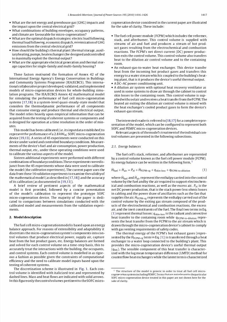
The discretization scheme is illustrated in Fig. 1. Each con-

trol volume is identified with italicized text and represented by

dashed lines. Mass and heat flows are indicated with solid arrows.

In this figureonly thecontrolvolumes pertinentto theSOFC micro-

cogeneration device considered in the current paper are illustrated

for the sake of clarity. These include:

• The fuel cell power module (FCPM) which includes the reformer,

stack, and afterburner. This control volume is supplied with

streams of air and fuel and produces a stream of hot prod-

uct gases resulting from the electrochemical and combustion

reactions. The FCPM’s net direct current (DC) power produc-

tion exits the control volume. This control volume also transfersheat to the dilution air control volume and to the containing

room.• An exhaust-gas-to-water heat exchanger. This device transfer

heat from the incoming hot product gases and transfers this

energy to a water stream whichis coupled to the building’s heat-

ing plant, that is it produces the device’s useful thermal output.• A DC–AC power conditioning unit.• A dilution air system with optional heat recovery ventilator as

used in some systems to draw air through the cabinet to control

skin losses to the containing room. This control volume is sup-

pliedwithcoolair andreceives a heat transfer from theFCPM. The

heated air exiting the dilution air control volume is mixed with

the heat exchanger’s cooled product gases to form the device’s

exhaust-gas stream.

Theinterested readeris referred to [18,17] f or a completerepre-

sentation of the model, which can be configured to represent both

SOFC and PEMFC micro-cogeneration devices.

Relevant aspects of themodel’s treatmentof theindividual con-

trol volumes are presented in the following subsections.

2.1. Energy balances

The fuel cell’s stack, reformer, and afterburner are represented

by a control volume known as the fuel cell power module (FCPM).

Its energy balance can be written in the following form,1

Hfuel + Hair = P el + HFCPM-cg + qskin-loss + qFCPM-to-dilution (1)

where Hfuel and Hair represent the enthalpy carried into the control

volume by the fuel andby the air required to support electrochem-

ical and combustion reactions, as well as the excess air. P el is the

net DC power production, that is the stack power less ohmic losses

in cabling and the power draw of ancillaries such as the fan that

supplies the air. HFCPM-cg represents the enthalpy carried out of the

control volume by the exiting gas stream composed of the prod-

ucts of the electrochemical and combustion reactions, the excess

air, and the inert constituents of the fuel. The final two terms in Eq.

(1) represent thermal losses: qskin-loss is the radiant and convective

heat transfer to the containing room while qFCPM-to-dilution repre-

sents the heat transfer from the FCPM to the air stream which is

drawn through the micro-cogeneration device’s cabinet to complywith gas venting requirements of safety codes.

The thermal energy of the FCPM’s hot exhaust gases (repre-

sented by the HFCPM-cg term in Eq. (1)) is transferred through a heat

exchanger to a water loop connected to the building’s plant. This

provides the micro-cogeneration device’s useful thermal output

(qHX). The sensible component of this heat transfer is character-

ized with the log mean temperature difference (LMTD) method for

counterflow heat exchangers while the latent term is characterized

1 The structure of the model is generic in order to treat all fuel cell micro-

cogeneration systemsincludingPEMFC.Terms thatare notrelevantto theparticular

SOFC micro-cogeneration device treated in this paper are not shown here for the

sake of clarity.



1418 I. Beausoleil-Morrison / Journal of Power Sources 195 (2010) 1416–1426

Fig. 1. Model discretization.

by estimating the rate of condensation. This is given by

qHX = qsensible + qlatent

= (UA)eff ·(T FCPM-cg − T w-out)− (T g-out − T w-in)

ln((T FCPM-cg − T w-out)/(T g-out − T w-in))

+ N H2O-cond · h fg

(2)

whereT FCPM-cg is the temperature of thehot gases exiting the FCPM

and entering the heat exchanger and T g-out is the temperature of

the cooled gases exiting the heat exchanger. T w-in is the temper-

ature of the cold water at the heat exchanger inlet and T w-out is

the temperature of the warmed water exiting the heat exchanger.

(UA)eff is the effective product of the heat transfer coefficient and

area (WK−1). N H2O-cond is the rate of condensation of water from

the gasstream (kmol s−1) and h fg is themolarheat of vapourization

of water (Jkmol−1).

A power conditioning system converts the FCPM’s DC output

to AC power to supply the building’s electrical loads and perhaps

to export power to the grid. A simple energy balance is used to

represent the control volume for this device

P AC = ÁPCU · P el (3)

where P AC represents the micro-cogeneration device’s AC power

production and ÁPCU is the DC–AC power conversion efficiency.

Eqs. (1)–(3) outline the methods used to characterize the energy

balances for three of the model’s control volumes. Similar tech-

niques are employed for the remaining six control volumes.

2.2. Empirical coefficients

There is a great deal of interdependency between the energy

balances representing each control volume as well as between the

individual terms of the energy balances. For example, the net DC

power production (appearing in Eqs. (1) and (3)) is related to the

fuel consumption (and thus the Hfuel term of Eq. (1)) through the

FCPM’s electrical efficiency

el =P el

N fuel · LHVfuel

(4)

where el is the electrical efficiency and N fuel is the molar flow rate

of the fuel.

Many of the individual terms of the energy balances are empir-

ical in nature and are evaluated on a time-step basis. For example,

the FCPM’s electrical efficiency required by Eq. (4) is given by,2

el = 0 + 1 · P el + 2 · P 2el (5)

where i are empirical coefficients.

Similarly, (UA)eff required in Eq. (2) is expressed as a parametric

relation of the water (N w) and gas (N g ) flow rates through the heat

exchanger

(UA)eff = hxs,0 + hxs,1 · N w + hxs,2 · N 2w + hxs,3 · N g + hxs,4 · N

2 g (6)

where hxs,i are empirical coefficients.

The DC–AC power conditioning efficiency is given byÁPCU = u0 + u1 · P el + u2 · P

2el (7)

where ui are empirical coefficients.

Expressions similar to Eqs. (5)–(7) are used to evaluate many of

the other terms in the energy balances on a time-step basis.

2.3. Solution procedure

At each time-step of a simulation (typically 1–5 min), the build-

ing simulation program invokes the fuel cell micro-cogeneration

2 Eq. (5) also contains terms that express degradation as a result of operational

time and stop–start cycling, but these are omitted here for the sake of clarity.




model and passes it a control signal requesting a given AC power

output (P AC). The fuel cell’s operating point is established by deter-

miningthe FCPM’s net DC power production (P el) through solution

of Eqs. (7) and (3). The electrical efficiency (el) is calculated with

Eq. (5) and the required fuel consumption (N fuel) determined with

Eq. (4). A polynomial expression is used to estimate theenthalpy of

each constituent of the fuel (CH4, C2H6, N2, etc.) as a functionof its

supply temperature [20]. This along with N fuel establishes the first

term of Eq. (1) energy balance. Clearly, any errors in the evaluation

of Eqs. (3)–(5), and/or (7) or in the i or ui empirical coefficients

will lead to errors in the determination of the fuel consumption.

Similar methods are used to establish the other terms of Eq. (1),

which is then solvedto yield theenthalpycarried outof the control

volume by the gas stream (HFCPM-cg). The composition of this gas

stream is determined by assuming complete reactions between the

fuel constituents and the air’s O2,

C xH y +

x+

y

4

·O2 → x · CO2 +

y

2·H2O (8)

When the flow rates of CO2 and H2O determined with Eq. (8)

are added to the flow rates of the non-reacting fuel and air con-

stituents, the composition and flow rate (N g ) of the product gas

stream are established. The polynomial function mentioned above

is then applied in an iterative manner to establish the tempera-ture (T FCPM-cg) corresponding to the value of HFCPM-cg solved by

Eq. (1). Clearly, any errors in the evaluation of any of the above-

mentionedequations (andothersnot mentionedhere)or anyerrors

in their empirical coefficients would lead to errors in the estimate

of T FCPM-cg.

This temperature is then used in the modelling of the heat

exchanger. Firstly, the flow rate of the product gas stream (N g ) is

used toestablish (UA)eff using Eq. (6). Eq. (2) is re-arranged and then

solved to determine the micro-cogeneration device’s useful ther-

mal output (qHX) and the heat exchanger’s exiting gas and water

temperatures. Once again, any errors in the evaluation of the many

terms that lead to N g and T FCPM-cg will propagate into errors in the

prediction of qHX.

3. Model calibration

The previous section outlined some of the model’s equations

requiring empirical coefficients (5)–(7). These coefficients are the

model’s inputs. The form of these empirical equations was cho-

sen to facilitate model calibration based upon the testing of

coherentfuel cellmicro-cogeneration systems. The calibration pro-

cess essentially involves the design and execution of experiments

that isolate the performance of specific aspects of the micro-

cogeneration system. Quantities are derived from the measured

data and regressions performed to establish the empirical coeffi-

cients.

As mentioned in the paper’s introduction, such a calibration

has been performed for a prototype micro-cogeneration sys-tem. The experimental configuration, types of instrumentation

employed,operating scenariosexamined, uncertainty analysis,and

data regression methods are detailed in [13].

Fig. 2 illustrates this effort’s calibration of Eq. (5). Seven exper-

iments were performed over a range of P el. For each of these 7

experiments, the value of P el was derived from two voltage mea-

surements and two current measurements (one pair to establish

the stack power production less cabling ohmic losses andthe other

the DC power draw of ancillaries). These derived P el values along

with measurements of N fuel were used to evaluate Eq. (4) to derive

the value of el for each of the 7 experiments. The value of LHV fuel

required by Eq. (4) was derived from the fuel’s composition as

determined through gas chromatography. The el values derived

from the measurements are plotted along the figure’s x-axis. The

Fig. 2. Eq. 5 versus measurements for calibration experiments.

Table 1

Goodness-of-fit metrics for calibrations of each equation term.

Average error Rms error Max error

el 0.4% 0.6% 1.2%

N air 2.3% 2.8% 5.6%

(UA)eff 1.9% 2.1% 3.2%

Heat exchanger condensation 11% 12% 21%

ÁPCU 0.1% 0.2% 0.2%

qFCPM-to-dilution 3.2% 3.9% 7.7%

qskin-loss ±20% of nominal value

error bars represent the uncertainty at the 95% confidence level, as

determined by propagating instrument bias errors and precision

indices using the methods described by [21,22] and as detailed in

[13].

Theexperimentsresulted in 7 pairs of derived el andP el values.

A non-linear regression of Eq. (5) was performedwith these data to

yield the calibrated i empirical coefficients. The el subsequently

determined with Eq. (5) using these calibrated i coefficients are

plotted on the y-axis of Fig. 2. Essentially this figure examines the

ability of Eq. (5) and the calibrated i coefficients to represent the

data from which the coefficients were derived. Table 1 presents

the average deviation (error) in el between the calibration and the

values derived from the measurements from the 7 experiments.It also presents the root-mean-square (rms) and the maximum

errors.

This calibration procedure was repeated for all terms pertinent

to this SOFC micro-cogeneration device.3Figs. 3 and 4 illustrate the

calibration of two of these terms. The former compares the cali-

brated air supply rate (see the second term of Eq. (1)) against the

measured values over the 28 experiments used in this calibration.

The latter compares the calibrated value of qFCPM-to-dilution (treated

as a constant value in the model) against the value derived from

measurements for the 7 experiments used in this calibration. The

3 The model is general in nature and as such includes control volumes and terms

not relevant to this particular device.




Fig. 3. N air calibration versus measurement for ca libration experiments.

uncertainty associated with this derived quantity is significant, for

reasons explained in [13].

Table 1 presents the goodness-of-fit metrics for these two cal-

ibrations, as well as those for most other calibrations pertinent to

the SOFC micro-cogeneration device. (The calibration of the FCPM’s

transientresponsecharacteristics are nottreated here as they have

no bearing upon the subject of the current paper.) An estimated

uncertainty rather than goodness-of-fit metrics are presented for

the qskin-loss term of Eq. (1) since it was determined from a sin-

gle experiment duringwhich infrared images were captured of the

micro-cogeneration device’s external surfaces. These were used toestimate surface temperatures and classic heat transfer relations

Fig. 4. qFCPM-to-dilution calibration versus measurement for cali bration experiments.

were used to estimate the free convection and longwave radiation

losses. The uncertaintyof thiscalibrationof thisterm wasestimated

to be 20% of its nominal value of 729 W.

Figs. 2–4 and Table 1 demonstrate that the calibrations of the

individual terms of the model accurately represent the calibration

data. Worthy of note are the significant uncertainties associated

with predicting condensation in the heat exchanger, as well as with

the dilution and skin loss heat transfer terms. A more rigorous test

of thequality or validity of thecalibration as well as the model itself

is presented in the next section.

4. Validation approach

4.1. Methodology

The validation of building simulation programs is a complex

and challenging field that has existed almost as long as building

simulation itself. Extensive efforts have been conducted under the

auspices of the International Energy Agency, the American Society

of Heating,Refrigerating, andAir-Conditioning Engineers, theEuro-

pean Committee for Standardization (CEN), and others to create

methodologies, tests, andstandards to verify the accuracy andreli-

ability of building simulation programs. Notable examples include[23–27].

In addition to providing consistent methods for comparing pre-

dictions from simulation programs, these initiatives have proven

effective at diagnosing errors: inadequacies of simplified math-

ematical models at representing the thermodynamic processes

occurring in reality; mathematical solution inaccuracies; and cod-

ing errors (bugs). A pragmatic approach composed of three primary

validation constructs to investigate these errors has been widely

accepted in the building simulation field [25]:

• Analytical verification.• Empirical validation.• Comparative testing.

The second and third methods have been employed to validate

the fuel cell micro-cogeneration model. Prior to empirically vali-

dating the model, comparative testing was performed to verify the

model implementations. The firstmethod, analytical validation,has

not been employed due to the complex nature of the devices and

the lack of appropriate analytic solutions for the relevant thermo-

dynamic processes.

A general principle applies to all three of these validation con-

structs.The simpler andmore controlled the test case,the easierit is

to identify and diagnose sources of error. Realisticcases are suitable

for testing the interactions between algorithms, but are less useful

for identifying and diagnosing errors. This is because the simulta-

neous operation of all possible error sources combined with the

possibility of offsetting errors means that good or bad agreementcannot be attributed to program validity.

4.2. Comparative testing

The fuel cell micro-cogeneration model has been indepen-

dently implemented into four simulation platforms. This provided

a unique opportunity to apply inter-model comparison testing to

diagnose mathematical solution and coding errors. A suite of 50

test cases, each carefully constructed to isolate a specific aspect of

the model, was created [28]. Collectively these test cases examine

every aspect of the model and exercise each line of its source code

implementations.

The comparison of simulation predictions between the four pro-

grams revealed numerous solution and coding errors that were




subsequently addressed. As a result, this exercise has verified the

implementations of the model: it can be stated with a high-degree

of confidence that the source code representations of the model

are error free. Consequently in conducting the empirical validation

work, any discrepancies between simulation predictions and mea-

surements couldbe attributed to inadequacies in the mathematical

model or to the calibration of its inputs.

5. Empirical validation

Section 4 discussed the technique used to verify the source-code

implementations of the model. One of the simulation platforms

assessed in this effort, ESP-r [29,30], is applied in this section.

Section 3 summarized how the model has been calibrated to

representthe performance of a 2.8 kWAC SOFC micro-cogeneration

device using experimental data from the calibration experiments.

The current section contrasts simulation predictions and mea-

surements that were taken in a disjunct set of experiments (the

validation experiments). Given the above argument, any observed

disagreement between simulation predictions and measurements

fromthese 16 validation experiments mustbe attributableto errors

in the mathematicalmodel and/or its calibration and/or in the mea-

surements.

5.1. Time-step comparisons for one experiment

Four boundary conditions fully define the operational state of

the micro-cogeneration device:

• The AC power production (see P AC in Eq. (3)).• The flow rate of water through the heat exchanger (see N w in Eq.

(6)).• The temperature of the cold water at the heat exchanger inlet

(see T w-in in Eq. (2)).• Thetemperature of the airsuppliedto the FCPM (see the Hair term

in Eq. (1)).

These boundaryconditions were maintained as constant as pos-

sible during each of the 16 validation experiments. Instantaneous

measurements of P el, N air, and N fuel were taken every second and

the averages over the minute were logged to file. All other mea-

surementsweretakenevery 15s andthe minutely averages logged.

Fig. 5 plots the 1-min averages of two of the boundary conditions

(P AC and T w-in) over the 10-min duration of one of the validation

experiments. The error bars in the figure represent the instrumen-

tation bias errors.

A simulation model was configuredto replicatethis experiment.

The boundary conditions supplied to the simulation model were

equivalenced to the 1-min-averaged measurements and a simula-

tion conducted with a 1-min time-step. This boundary condition

equivalencing is illustrated in Fig. 5.By equivalencing the boundary conditions, direct comparisons

could then be made between the simulation predictions and the

measurements. In keeping with the accepted validation method-

ology’s tenet of simplicity, the FCPM’s net DC power production

(P el) is the first parameter compared. P el is calculated with Eqs. (3)

and (7) using the ui coefficients and subject to the P AC boundary

condition. Therefore, disagreement between the simulation pre-

dictions and the measurements would indicate that either or both

of these equations were inadequate to represent the performance

of the system, that the calibration of the ui empirical coefficients

was deficient, or that there were inaccuracies in the solution of the

equations.

The top-left corner of Fig.6 compares the simulationpredictions

of P el to the measurements. For presentation clarity the measured

Fig. 5. Equivalencing simulation boundary conditions to replicate measurements.

and simulated quantities have been slightly offset from each other

along the x-axis. The errorbars associatedwith themeasuredpoints

represent instrumentation bias errors.

The figure also includes error bars on the simulation predic-

tions. Section 3 describedthe procedures thatwere usedto calibrate

the model using measured data. The model’s equations did not

perfectly regress these measured data. For example, it was found

that the calibrated ui coefficients could result in up to 0.2% error

(see Table 1) in the prediction of ÁPCU using Eq. (7). Furthermore,

uncertainty in the simulation program’s prescribed P AC boundary

condition would propagate into the prediction of P el using Eq. (3),augmenting the uncertainty in the application of Eq. (7). These

uncertainties were propagated using a root-sum-square method

[21,22] to estimate the uncertainty associated with the simula-

tion predictions. Thus the error bars associatedwith the simulation

predictions represent the combined uncertainty due to boundary

conditions and calibration inaccuracies.

As can be seen from the top-left corner of the figure, the

simulation predictions agree with the measurements within the

uncertainty associated with the boundary conditions and cali-

bration. Furthermore, the simulation predictions agree with the

measurements within the instrumentation bias error at 7 of the

10 1-min intervals. The exception occurs at both the beginning

and end of the experiment, where the simulation produces a

slightly greater variation in P el from one time-step to the next.(Note the scale of the y-axis.) Notwithstanding, the average, rms,

and maximum deviation between the simulation predictions and

measurements indicates excellent agreement overall (see Table 2).

These goodness-of-fit metrics show slightly higher deviation than

Table 2

Goodness-of-fit metrics for time-step simulation predictions for 1 of the 16 valida-

tion experiments.


P el 0.3% 0.4% 0.8%

N fuel 2.2% 2.2% 2.9%

(UA)eff 1.4% 1.7% 3.5%

qHX 6.7% 6.7% 8.0%




Fig. 6. Time-step comparisons of four key simulation predictions for one experiment.

were observed with the calibration of Eq. (7) (see Table 1) and

higher deviation than seen with the P AC boundary condition. How-

ever, it can be statedthat agreementis very good,with a maximum

deviation between simulation and measurement of less than 1%.

The comparisons illustrated in Fig.6 involve greater interactions

between algorithms (i.e. less simplicity) as one moves from left to

right and from top to bottom. The top-right corner compares the

simulation predictions of the fuel consumption to the measure-

ments.This comparison examines thesame aspects of the model as

the precedingP el comparison, in addition to Eqs. (4)and (5) and the

i empirical coefficients (refer to Section 2.3). Once again, the sim-

ulation predictions agree withthe measurements within the model

uncertainty at each of the 1-min intervals. The instrumentation

bias error is only 2% of the measured gas flow for this experiment.

Notwithstanding, the simulation predictions agree with the mea-

surements within the instrumentation bias error at a number of

the 10 1-min intervals and the goodness-of-fit metrics indicate an

excellent prediction overall (see Table 2).

The bottom-left corner of Fig. 6 compares the simulation pre-

dictions of the heat exchanger’s (UA)eff value to the measurements.

This examines the validity of the form of Eq. (6) and the hxs,i coef-

ficients. It is worth noting that there was no condensation of water

Fig. 7. Time-averaged comparisons of four key simulation predictions for the 16 validation experiments.




Table 3

Goodness-of-fit metrics for simulationpredictions for the 16 time-averaged valida-

tion experiments.


P el 0.2% 0.2% 0.5%

N fuel 1.2% 1.9% 6.1%

(UA)eff 5.4% 6.0% 9.5%

qHX 7.9% 8.4% 12.2%

Ánet-AC 1.2% 1.8% 5.8%

Áth 8.5% 8.8% 13%Ácogen 5.3% 5.6% 8.9%

vapour within the heat exchanger during this experiment. In addi-

tion, it stresses the aspects of the model that establish N g . The

simulation predictions agree with the measurements within both

the model uncertainty and the instrumentation bias error at each

of the 10 1-min intervals. The goodness-of-fitmetrics are similar in

magnitude to those for the calibration of the hxs,i coefficients (see

Table 1).

The bottom-right corner of Fig. 6 compares the simulation pre-

dictions of the useful thermal output (qHX) to the measurements.

This examines the combined influence of most aspects of the

model. Of particular significance is the large uncertainty associ-

ated with the qskin-loss and qFCPM-to-dilution terms of Eq. (1) energybalance. Although all measurements lie within the model’s uncer-

tainty, as can be seen in the figure, the simulation predictions

lie outside the measurement bias uncertainty at all points. How-

ever, the goodness-of-fit metrics given in Table 2 are reasonable

given the uncertainty associated with the calibration of the two

aforementioned heat loss terms: the maximum deviation between

simulation predictions and the heat flow derived from measure-

ments is 8%.

5.2. Time-averaged comparisons for 16 validation experiments

The 16 validation experiments varied in duration from 10 min

to over 10 h (long experiments were required when condensation

formed in the heat exchanger for reasons explained in [13]). Thenear-constant boundary conditions were time-averaged over each

experiment and a simulation model was configured to equivalence

these conditions.This resulted in simulation predictions for 16 sets

of time-averagedboundary conditions. Averages were thenformed

from the measured data sets for the same parameters previously

examined in the single experiment.

These comparisons are illustrated in Fig. 7. The quantities

derived from the measurements are plotted along the x-axis while

the simulation predictions are plotted on the y-axis. The diagonals

represent the line of perfect agreement. The error bars in the x-

direction represent the uncertainty at the 95% confidence level of

the time-averaged quantities derived from the measurements. The

error bars in the y-direction represent the estimated uncertainties

of the model due to uncertainties in boundary conditions and thecalibrations. The goodness-of-fit metrics are presented in Table 3.

The top-left corner of Fig. 7 compares the simulation predic-

tions of P el to the measurements. The simulation predictions agree

with the measurements within the model uncertainty for all 16

experiments. Furthermore, the model agrees with the measure-

ments within the measurement uncertainly at the 95% confidence

level for 14 of the 16 experiments. In one of the outlying experi-

ments the simulation prediction is within2 W of the measurement

uncertainty whereas in the other it is within 1 W.

In general terms, the simulation predictions deviate further

from the measurements as complexity increases. Moving from left

to right on the graph and from top to bottom involves greater

interaction between algorithms and this affords the possibility of

uncertainty propagation. Notwithstanding, for 13 of the 16 exper-

Fig. 8. Exhaust-gas-to-water heat exchanger.

iments the simulation predicts the fuel consumption to within the

measurement uncertainty at the 95% confidence level (top-right

corner). In all experiments the simulation predicts the fuel con-

sumption within the model uncertainty.And for all 16 experiments

the simulation predicts the heat exchanger’s (UA)eff to within both

themodel and themeasurementuncertaintyat the95% confidence

level (bottom-left corner).

Although theqHX predictions generallyagree withthe measure-

ments within the model uncertainty (see bottom-right corner of

Fig. 7), it appears that there might be a systematic bias. For 15

of the 16 experiments the simulation predicts less heat transfer

that the value derived from the measurements and in all but two

experiments the simulation predictions lie outside the measure-

mentuncertainty at the95% confidence level. The averagedeviation

between the simulation predictions and the values derived from

measurements is 330W (∼8%) and in one experiment the differ-

ence is more than 600 W (12%). The four experiments in which

water vapourfrom thegas streamcondensed in theheat exchanger

produced the greatest values of qHX. These experiments show some

of the greatest deviation between simulation predictions and mea-

surements. As explained earlier there is considerable uncertainty

associated with the calibration of this aspect of the model (refer to

Table 1).

Further analysis of the measured data wasperformed to explore

this potential systematic bias. This is best explained by examin-

ing the schematic representation of the heat exchanger given in

Fig. 8. In the previous work [13] the temperatures of all four state

points illustrated in this figure (two in the gas stream, two in the

liquid water stream) were used to calibrate the heat exchanger’s(UA)eff (refer to the sensible term in Eq. (2)). The model assumes

that the heat loss from theheatexchanger to the ambient is negligi-

bleand that the heat capacityof each fluid streamremains constant

through the heat exchanger. Consequently, when no condensation

is forming theheat transfer from the hotproductgasesto theliquid

water streamcan be calculated with measurements of only the two

liquid water state points or only the two gas state points, that is

qHX = (N cP )w(T water-out − T water-in) = (N cP ) g (T FCPM-cg − T g-out) (9)

where (N cP )w is the product of flow rate(kmol s−1) andheat capac-

ity (J kmol−1 K) of the liquid water stream flowing through the

heat exchanger; (N cP ) g corresponds to these quantities of the gas

stream.




Fig. 9. Contrast of qHX derived from measurements from heat exchanger’s liquid

water and gas streams.

The qHX values plotted in Fig. 7 are derived from flow rate and

temperature measurements taken on the water stream side of the

heat exchanger (the left side of Eq. (9). To explore the apparent

systematic bias revealed in the bottom-right corner of Fig. 7 the

qHX values were derived again, but this time using the flow rate

and temperature measurements taken on the gas side of the heat

exchanger (the right side of Eq. (9)). The result of this analysis is

illustrated in Fig. 9. For each of the 12 experiments during which

there was only sensible heat transfer, this figure contrasts the qHX

values derived from the two sets of measurements. It also plotsthe qHX value predicted by simulations with the calibrated model.

Once again, for presentationclarity thethree sets of data have been

slightly offset from each other along the x-axis.

Ascanbeseen,inmostoftheexperimentsthereisaconsiderable

discrepancy between the water-side and gas-side measurements.

In all cases, measurements taken on the water side of the heat

exchanger resulted in higher values of qHX (by up to 750W). How-

ever, in the majority of experiments the water-side and gas-side

measurements agreed within the measurement uncertainty at the

95% confidence level. In 11 of the 12 experiments the simulation

predictions lay in between the values derived from the water and

gas stream measurements. And in all cases the range of the model

uncertainty overlaps with the uncertainty ranges of the measured

data.Based upon these observations it is possible that the error bars

in the bottom-right of Fig. 7 underestimate the true experimen-

tal uncertainty. These error bars, representing the uncertainty at

the 95% confidence interval, were calculated through the propa-

gation of bias errors and measurement precision indices through

a root-sum-square method [21,22]. The bias errors were estab-

lished mainly based upon instrumentation specifications. In some

casesinstrumentswere calibratedand in other casesadditionalbias

errors were assigned based upon judgement. As such, the uncer-

tainty bars in the figure represent the errors associated with two

calibrated type-T thermocouples (bias errors of 0.1 ◦C) that mea-

sured T w-in and T w-out and a water flow meter to measure N w (bias

error of ∼2%). It is possible that the instrumentation bias errors

mayhave in fact been greater than the manufacturer specifications

Fig. 10. Time-averaged comparisons of net AC, thermal, and cogeneration efficien-

cies for the 16 validation experiments.

or instrumentation calibration estimates. Or, that the placement of

one or more of the thermocouples may have biased the readings,

i.e. it may not have been reading the intended state point.

The final check on the model’s validity is made through exam-

ining the predictions of three key outputs, the net efficiencies

for electrical, useful thermal, and total output from the micro-

cogeneration device

Ánet-AC=

P AC

N fuel · LHVfuel

(10)

Áth =qHX

N fuel · LHVfuel

(11)

Ácogen = Ánet-AC + Áth (12)

These three efficiency values would be of prime importance

in a simulation-based assessment of the performance of micro-

cogeneration systems. As their calculation depends upon the

interactionof allaspects of themodel, this is perhaps themostchal-

lenging comparison of simulation predictions to measurements.

The comparison of the simulation predictions of these quantities

with the values derived from the measurements are illustrated in

Fig. 10 and the goodness-of-fit metrics are presented in Table 3.The thermal efficiencies are derived from the measurements on

the liquid water stream using the left side of Eq. (9).

As canbe seen,simulation predictions of the electrical efficiency

are in better agreement than those for the thermal efficiency. As

explained earlier, the error bars representing the uncertainty at the

95% confidence interval possibly underestimate the experimental

uncertainty in deriving the thermal efficiency. Notwithstanding,

the simulation predictions of the thermal efficiency agree with

the measurements within the uncertainly at the 95% confidence

level for 5 of the 16 experiments and the measurement and model

uncertainties overlap for all experiments. And for 11 of the 16

experiments the simulation predicts the total efficiency within the

measurement uncertainty at the 95% confidence level while the

measurements are within the model uncertainty in all cases.




6. Conclusions

This paper has examined the validity of a mathematical

model—and its calibration to a particular device—for simulating

the performance of SOFC micro-cogeneration systems. Pertinent

aspects of the mathematical model were described and the meth-

ods used to calibrate the model (i.e. establish its inputs) using

data gathered through 45 experiments conducted with a proto-

type 2.8 kWAC

SOFC micro-cogeneration device were presented.

The methodology used to validate the model, including verifying

its implementation into the source code of building simulation

programs, was then elaborated. This described how inter-model

comparative testing was used to eliminate coding and solution

errors.

The paper then described how measured data from 16 exper-

iments (disjunct from the 45 experiments used to calibrate the

model) were used to empirically validate the model and its cal-

ibration. It showed how simulations were equivalenced with

experimental conditions and how measured values and quantities

derived from the measurements were compared to simulation pre-

dictions. The propagation of measurement uncertainties as well

as the propagation of uncertainties in boundary conditions and

calibration coefficients into model predictions were considered in

these comparisons. These comparisons spanned a range of modelparameters, progressing from the simplest case in which only a

small subset of the model was exercised, to the complex which

involved the concurrent operation and interaction of all aspects of

the model.

The paper identified the aspects of the model with the great-

est uncertainty, that is the calculation of parasitic thermal losses

and the condensation of the exhaust-gas’ water vapour within the

heat recovery device. The paper explained how this uncertainty

could propagate errors into simulation predictions of the useful

thermal output. Although this parameter produced the greatest

deviations between measurements and simulation predictions, the

predictions generally agree with the measurements within the

model uncertainty. And in all experiments the range of model

uncertainty overlaps with the uncertainty ranges of the measureddata.

Good agreement between simulation predictions and measure-

ments was found for other key parameters (e.g. net DC power

production, rate of fuel consumption, energy conversion efficien-

cies) over the range of the 16 experiments. Consequently, it is

concluded that the form of the mathematical model can accurately

represents the performance of SOFC micro-cogeneration devices

and theirsub-systems. Furthermore, it has been demonstrated that

with the calibration constants determined by [13] the calibrated

model can accurately represent the performance of a prototype

2.8 kWAC SOFC micro-cogeneration device. Detailed performance

assessments can now be performed using this calibrated model to

examine the applicabilityof this device for supplyingbuildingelec-

trical and thermal energy requirements. Additionally, the modelcan be calibrated to represent the performance of other prototype

SOFC micro-cogeneration devices using the techniques elaborated

by [13].

Acknowledgements

The work described in this paper was undertaken as part of

IEA/ECBCS Annex 42 Simulation of Building-Integrated Fuel Cell

and Other Cogeneration Systems (http://www.cogen-sim.net). The

Annex was an international collaborative research effort and the

author gratefully acknowledges the indirect or direct contributions

of the other Annex participants. The contributions of Mr. Stephen

Oikawa in conducting the experiments and of Ms. Kathleen Lom-

bardi in analyzing the measured data are greatly appreciated. The

anonymous reviewers are thanked for their insightful critique and

helpful suggestions.

References

[1] I. Knight, V. Ugursal (Eds.), Residential Cogeneration Systems: A Review of the Current Technologies, IEA/ECBCS Annex 42 Report, 2005. ISBN No. 0-662-40482-3.

[2] H. Onovwiona, V. Ugursal, Residential cogeneration systems: review of thecurrent technology, Renewable and Sustainable Energy Reviews 10 (5) (2006)

389–431.[3] G. Gigliucci, L. Petruzzi, E. Cerelli, A. Garzisi, A.L. Mendola, Demonstration of a

residential CHP system based on PEM fuel cells, Journal of Power Sources 131(1–2) (2004) 62–68.

[4] Y. Hamada, M. Nakamura, H. Kubota, K. Ochifuji, M. Murase, R. Goto, Field per-formance of a polymer electrolyte fuel cell for a residential energy system,Renewable and Sustainable Energy Reviews 9 (4) (2005) 345–362.

[5] Y. Hamada, R. Goto,M. Nakamura,H. Kubota, K. Ochifuji, Operatingresults andsimulations on a fuel cell for residential energy systems, Energy Conversionand Management 47 (20) (2006) 3562–3571.

[6] W. Münch,H. Frey, M. Edel, A. Kessler,Stationary fuel cells-results of 2 years of operation at EnBW, Journal of Power Sources 155 (1) (2006) 77–82.

[7] M.Radulescu,O. Lottin, M.Feidt, C.Lombard,D.Le Noc, S.Le Doze,Experimentaland theoretical analysis of the operation of a natural-gas cogeneration systemusing a polymer exchange membrane fuel cell, Chemical Engineering Science61 (2) (2006) 743–752.

[8] M. Davis, A. Fanney, M. LaBarre,K. Henderson, B. Dougherty,Parametersaffect-ing the performance of a residential-scale stationary fuel cell system, Journal

of Fuel Cell Science and Technology 4 (2) (2007) 109–115.[9] M. Davis, Measured performance of three residential fuel cell systems, in:Micro-cogeneration, Proc. 2008, Ottawa, Canada, 2008.

[10] K. Kobayashi, Performance of residential PEMFC cogeneration system in annualactual use, in: Proceedings of the Micro-cogeneration 2008, Ottawa, Canada,2008.

[11] H. Miura,H. Habara, T. Sawachi, M. Mae, Y. Kuwasawa,Development ofevalua-tion method for microco-cogeneration in Japanby validationexperiment. Part2. Evaluation of actual performance of PEFC by experiments with occupants’lifestyle simulator, in: Proceedings of the Micro-Cogeneration 2008, Ottawa,Canada, 2008.

[12] H.-S. Chu, F. Tsau, Y.-Y. Yan, K.-L. Hsueh,F.-L.Chen, Thedevelopment ofa smallPEMFC combined heat and power system, Journal of Power Sources 176 (2)(2008) 499–514.

[13] I. Beausoleil-Morrison, K. Lombardi, The calibration of a model for simulat-ing the thermal and electrical performance of a 2.8 kwAC solid-oxide fuel-cellmicro-cogeneration device, Journal of Power Sources 186 (1) (2009) 67–79.

[14] G. Mulder, P. Coenen, A. Martens, J. Spaepen, The development of a 6kw fuel

cell generator based on alkaline fuel cell technology, International Journal of Hydrogen Energy 33 (12) (2008) 3220–3224.

[15] U.C. Colpier,D. Cornland,The economicsof thecombined cyclegas turbine—anexperience curve analysis, Energy Policy 30 (4) (2002) 309–316.

[16] T. DeMoss, Theyre he-e-re (almost): the 60% efficient combined cycle, PowerEngineering 100 (7) (1996) 17–21.

[17] I. Beausoleil-Morrison, A. Schatz, F. Maréchal, A model forsimulating thether-mal and electrical production of small-scale solid-oxide fuel cell cogenerationsystems within building simulation programs, Journal of HVAC&R ResearchSpecial Issue 12 (3a) (2006) 641–667.

[18] N. Kelly, I. Beausoleil-Morrison(Eds.),Specifications forModellingFuel CellandCombustion-Based Residential Cogeneration Devices within Whole-BuildingSimulation Programs, IEA/ECBCS Annex 42 Report, 2007. ISBN No. 978-0-662-47116-5.

[19] I. Beausoleil-Morrison(Ed.), Experimental Investigations of Residential Cogen-eration Devices and ModelCalibration, IEA/ECBCSAnnex 42 Report, 2007.ISBNNo. 978-0-662-47523-1.

[20] P. Linstrom, W. Mallard (Eds.), NIST Chemistry WebBook, NIST Standard Ref-erence Database Number 69, National Institute of Standards and Technology,

Gaithersburg, USA.[21] R. Moffat, Describing the uncertainties in experimental results, Experimental

Thermal and Fluid Science 1 (1988) 3–17.[22] R.Abernethy, R. Benedict,R. Dowdell, ASMEmeasurementuncertainty, Journal

of Fluids Engineering 107 (1985) 161–164.[23] S. Jensen (Ed.), Validation of Building Energy Simulation Programs, Part I and

II, PASSYS Subgroup Model Validation and Development, 1993. eUR 15115 EN.[24] K. Lomas, H. Eppel, C. Martin, D. Bloomfield, Empirical Validation of Thermal

Building Simulation Programs Using Test Room Data, vol. 1: Final Report, IEAECBCS Annex 21 and IEA SHC Task 12, 1994.

[25] R. Judkoff, J. Neymark,InternationalEnergyAgency Building Energy SimulationTest (BESTEST) and Diagnostic Method, IEA/ECBCS Annex 21 Subtask C andIEA/SHC Task 12 Subtask B Report, 1995.

[26] CEN, prEN ISO 13791: Thermal Performance of Buildings Calculation of Inter-nal Temperatures of a Roomin Summer Without MechanicalCooling—GeneralCriteria and Validation Procedures, ISO/FDIS 13791:2004, Brussels, Belgium,2004.

[27] ANSI/ASHRAE, Standard Method of Test for the Evaluation of Building Energy

Analysis Computer Programs, Standard 140-2007, Atlanta, USA, 2007.

http://www.cogen-sim.net/

http://www.cogen-sim.net/




[28] I. Beausoleil-Morrison, B. Griffith, T. Vesanen,A. Weber, A demonstrationof theeffectiveness of inter-program comparative testing for diagnosing and repair-ing solution and coding errors in building simulation programs, Journal of Building Performance Simulation 2 (1) (2009) 63–73.

[29] ESRU, TheESP-r systemfor building energy simulations: user guide version 10series, Tech. Rep. U05/1, University of Strathclyde, Glasgow, UK, 2005.

[30] J. Clarke, Energy Simulation in Building Design, 2nd ed., Butterworth-Heinemann, Oxford, UK, 2001.

Beausoleil 2010, The Empirical Validation of a Model

Documents

Transcript of Beausoleil 2010, The Empirical Validation of a Model