BD Single-Cell Genomics Bioinformatics Handbook

Doc ID: 54169 Rev. 7.0

23-21713-0007/2019

For Research Use Only

Becton, Dickinson and CompanyBD Biosciences2350 Qume DriveSan Jose, CA 95131 USATel 1.877.232.8995, prompt 2, 2

[email protected]

BD® Single-Cell GenomicsBioinformatics Handbook

Doc ID: 54169 Rev. 7.0

Copyrights/trademarks

BD, the BD Logo and Rhapsody are trademarks of Becton, Dickinson and Company or its affiliates. All other trademarks are the property of their respective owners. © 2019 BD. All rights reserved.

The information in this guide is subject to change without notice. BD Biosciences reserves the right to change its products and services at any time to incorporate the latest technological developments. Although this guide has been prepared with every precaution to ensure accuracy, BD Biosciences assumes no liability for any errors or omissions, nor for any damages resulting from the application or use of this information. BD Biosciences welcomes customer input on corrections and suggestions for improvement.

Regulatory information

For Research Use Only. Not for use in diagnostic or therapeutic procedures.

History

Revision Date Changes made

Doc ID: 54169 Rev. 1.0 09/2017 Initial release.

Doc ID: 54169 Rev. 2.0 11/2017 —Added content on sample multiplexing. See Step 7. Determine the sample of origin (sample multiplexing only) (page 31) and Reviewing sequencing analysis output files (page 37).

—Added content on specifying gene targets.

Doc ID: 54169 Rev. 3.0 01/2018 —Updated content of BD Data View to v1.1, which includes these new features: New color options for plots, highlight selected annotated groups in plots, filter data table by cells based on gene expression, new calculation on fold changes and mean gene expression, new option to modify data table names and annotation list names.

—Added two examples for use with BD Data View.

—Expanded information on selecting a transcript, selecting primers, and output files.

Doc ID: 54169 Rev. 4.0 04/2018 —Added another example for use with BD Data View.

Doc ID: 54169 Rev. 5.0 07/2018 —Added metrics outputs for BD™ AbSeq. See BD Rhapsody™ sequencing analysis (page 9)

—Updated to BD Data View v1.2. Some new features include:–Automatic detection of AbSeq markers in data tables–New Gene A v. Gene B feature to compare two gene markers

–Combine one or more data tables

–Differential expression of >1,500 genes

Doc ID: 54169 Rev. 6.0 10/2018 —Updated cross references from system user guides to instrument user guides.

—Changed content to say that a BAM file is sorted according to the alignment coordinates of R2 reads on each chromosome. See BAM and BAM Index (page 50).

—Added recommendation to analyze datasets that are ≤1TB in size. See Understanding the BD Rhapsody Analysis pipeline step-by-step (page 11).

—Updated output file name in example to Combined_<sample_multiplex_name>_DBEC_MolsPerCell.csv.

Doc ID: 54169 Rev. 7.0

23-21713-00

07/2019 —Added content for BD Rhapsody™ System Whole Transcriptome Analysis (WTA).

—Updated some step parameters.

—Revised recommendation to analyze datasets from ≤1 TB to ≤100 GB.

Revision Date Changes made

Doc ID: 54169 Rev. 7.0

Contents

Chapter 1: Introduction 7

About this handbook . . . . . . . . . . . . . . . . . . . . . . . . . . . . . . . . . . . . . . . . . . . . . . 8

Chapter 2: BD Rhapsody™ sequencing analysis 9

How to use this chapter . . . . . . . . . . . . . . . . . . . . . . . . . . . . . . . . . . . . . . . . . . . 10

Understanding the BD Rhapsody Analysis pipeline step-by-step . . . . . . . . . . . . . 11

Step 1. Filter by read quality . . . . . . . . . . . . . . . . . . . . . . . . . . . . . . . . . . . . . . . . 14

Step 2. Annotate R1 reads . . . . . . . . . . . . . . . . . . . . . . . . . . . . . . . . . . . . . . . . . 14

Step 3. Annotate R2 reads . . . . . . . . . . . . . . . . . . . . . . . . . . . . . . . . . . . . . . . . . 16

Step 4. Combine information from R1 and R2 annotations . . . . . . . . . . . . . . . . 17

Step 5. Annotate molecules . . . . . . . . . . . . . . . . . . . . . . . . . . . . . . . . . . . . . . . . . 17

Step 6. Determine putative cells . . . . . . . . . . . . . . . . . . . . . . . . . . . . . . . . . . . . . 23

Step 7. Determine the sample of origin (sample multiplexing only) . . . . . . . . . . . . . . . . . . . . . . . . . . . . . . . . . . . . . . . . . 31

Step 8. Generate expression matrices . . . . . . . . . . . . . . . . . . . . . . . . . . . . . . . . . 35

Step 9. Annotate BAM . . . . . . . . . . . . . . . . . . . . . . . . . . . . . . . . . . . . . . . . . . . . 36

Step 10. Generate metrics summary . . . . . . . . . . . . . . . . . . . . . . . . . . . . . . . . . . 36

Step 11. Clustering analysis . . . . . . . . . . . . . . . . . . . . . . . . . . . . . . . . . . . . . . . . 36

Reviewing sequencing analysis output files . . . . . . . . . . . . . . . . . . . . . . . . . . . . . 37

Assessing BD Rhapsody library quality with skim sequencing . . . . . . . . . . . . . . 64

Interpreting output metrics . . . . . . . . . . . . . . . . . . . . . . . . . . . . . . . . . . . . . . . . . 65

References . . . . . . . . . . . . . . . . . . . . . . . . . . . . . . . . . . . . . . . . . . . . . . . . . . . . . . 70

BD Single-Cell Genomics Bioinformatics Handbook6

Doc ID: 54169 Rev. 7.0

Chapter 3: BD Rhapsody™ Targeted clustering analysis 73

Clustering Analysis Workflow . . . . . . . . . . . . . . . . . . . . . . . . . . . . . . . . . . . . . . . 74

Reviewing clustering analysis output files . . . . . . . . . . . . . . . . . . . . . . . . . . . . . . 79

References . . . . . . . . . . . . . . . . . . . . . . . . . . . . . . . . . . . . . . . . . . . . . . . . . . . . . . 86

Chapter 4: Glossary 87

Doc ID: 54169 Rev. 7.0

1Introduction

Doc ID: 54169 Rev. 7.0


About this handbookIntroduction This handbook is a comprehensive reference to help you prepare

and analyze single-cell libraries with the BD Rhapsody™ Single-Cell Analysis system or the BD Rhapsody™ Express Single-Cell Analysis system. Major aspects of the BD single-cell genomics bioinformatics workflow are covered. This reference explains the BD single-cell genomics sequencing and clustering algorithms to deepen your understanding of how single-cell mRNA and protein (AbSeq) expression profiles are generated and clustered. In addition, the handbook defines every analysis metric.

The BD single-cell genomics team

Doc ID: 54169 Rev. 7.0


2BD Rhapsody™ sequencing

analysis

Doc ID: 54169 Rev. 7.0


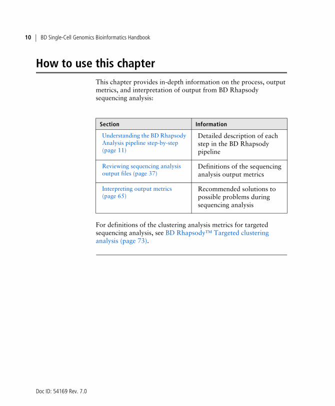
How to use this chapterThis chapter provides in-depth information on the process, output metrics, and interpretation of output from BD Rhapsody sequencing analysis:

For definitions of the clustering analysis metrics for targeted sequencing analysis, see BD Rhapsody™ Targeted clustering analysis (page 73).

Section Information

Understanding the BD Rhapsody Analysis pipeline step-by-step (page 11)

Detailed description of each step in the BD Rhapsody pipeline

Reviewing sequencing analysis output files (page 37)

Definitions of the sequencing analysis output metrics

Interpreting output metrics (page 65)

Recommended solutions to possible problems during sequencing analysis

Doc ID: 54169 Rev. 7.0


Understanding the BD Rhapsody Analysis pipeline step-by-stepIntroduction This section provides an in-depth description of each step in the

BD Rhapsody Analysis pipelines.

For instructions on running the pipeline, see the BD Single-Cell Genomics Analysis Setup User Guide (Doc ID: 47383).

Genomics technical publications are available for download from the BD Genomics Resource Library at bd.com/genomics-resources.

BD Biosciences recommends analyzing datasets that are ≤100 GB in size. For datasets (compressed FASTQ FILES from all libraries) >100 GB, contact BD Biosciences technical support at [email protected].

Overview The BD Rhapsody™ assays are used to create sequencing libraries from single-cell multiomic experiments.

The analysis pipeline works with paired-end FASTQ R1 and R2 files generated from Illumina sequencers. The minimum read length required is 60 bp for R1 and 42 bp for R2. R1 reads contain information on the cell label and molecular identifier, and R2 reads contain information on the gene. See Figure 1.

Figure 1. Structure of read pair that is generated by sequencing the libraries prepared with BD Rhapsody assays.

cDNA

R1 read

R2 read

poly TUMICell label

mailto: [email protected]

http://www.bd.com/genomics-resources

mailto: [email protected]

Doc ID: 54169 Rev. 7.0


Targeted Overview After sequencing, the targeted analysis pipeline takes the FASTQ files, an mRNA reference file, and an AbSeq reference file (if the latter is required) for gene alignment. See Figure 2.

Figure 2. Overview of the steps in the targeted analysis pipeline. For definitions of terms, see Glossary (page 87).

R1 FASTQ

Read quality filtering

R2 FASTQ

Read quality filtering

Filtered R1 Filtered R2

Valid read pairs

Raw molecules

RSEC adjusted molecules

DBEC adjusted molecules

Single cell gene expression profiles

Cluster assignment and representative features

Collapse reads to raw molecules

RSEC MI adjustment

DBEC MI adjustment

Cell label filtering

Clustering analysis

Process that filters out reads

Process that does not filter reads

Input / output of a process

Legend:

Sequencing analysis

Clustering analysis

Sample determination

Putative cells

Sample multiplexing(optional)

Doc ID: 54169 Rev. 7.0


WTA Overview After sequencing, the WTA pipeline takes the FASTQ files, a reference genome, and a transcriptome annotation file. See Figure 3.

Figure 3. Overview of the steps in the WTA analysis pipeline. For definitions of terms, see Glossary (page 87).

The next sections describe the analysis pipeline step-by-step.

R1 FASTQ

Read quality ltering

R2 FASTQ

Read quality ltering

Filtered R1 Filtered R2

Valid read pairs

Raw molecules

RSEC adjusted molecules

Single cell gene expression pr es

Collapse reads to raw molecules

RSEC MI adjustment

Cell label tering

Process that lters out reads

Process that does not lter reads

Input / output of a process

Legend:

Sequencing analysis

Sample determina on

Puta ve cells

Sample multiplexing(optional)

Doc ID: 54169 Rev. 7.0


Step 1. Filter by read qualityFiltering criteria Read pairs with low sequencing quality are first removed. This step

reduces the influence of poor sequencing quality from the metrics that are specific to the BD Rhapsody assays.

The following filtering criteria are applied to each read pair:

• Read length: If the length of R1 read is <60 bp or R2 read is <42 bp, the R1/R2 read pair is dropped.

• Mean base quality score of the read: If the mean base quality score of either R1 read or R2 read is <20, the read pair is dropped.

• Highest Single Nucleotide Frequency (SNF) observed across the bases of the read: If SNF is ≥0.55 for the R1 read or SNF ≥0.80 for the R2 read, the read pair is dropped. This criterion removes reads with low complexity such as strings of identical bases and tandem repeats.

The thresholds for each filter are determined empirically.

Step 2. Annotate R1 readsR1 structure The quality-filtered R1 reads are analyzed to identify the cell label

section sequence (CLS), common sequences (L), Unique Molecular Identifier (UMI) sequence, and if applicable, poly(T) tail. See Figure 4.

Figure 4. Structure of R1 read.

CLS1 L1 CLS2 L2 CLS3 UMI poly T�

��

��

� � � ��

��

Doc ID: 54169 Rev. 7.0


Cell label Information of the cell label is captured by bases in three sections (CLS1, CLS2, CLS3) along each R1 read. Two common sequences (L1, L2) separate the three CLSs, and the presence of L1 and L2 relates to the way the capture oligonucleotide probes on the beads are constructed. By design, each CLS has one of 96 predefined sequences, which has a Hamming distance of at least four bases and an edit distance of at least two bases apart. A cell label is defined by the unique combination of predefined sequences in the three CLSs. Thus, the maximum possible number of cell labels is 963 (884,736). A cell label is represented by an index between 1–963.

Reads are first checked for perfect matches in all three pre-designed CLS sequences at the expected locations, CLS1: position 1–9, CLS2: position 22–30, and CLS3: position 44–52. Reads with perfect matches are kept.

The remaining reads are subjected to another round of filtering to recover reads with base substitutions, insertions, deletions caused by sequencing errors, PCR errors, or errors in oligonucleotide synthesis.

UMI By design, the UMI is a string of eight randomers immediately downstream of CLS3. If the CLSs have perfect matches or base substitutions, the UMI sequence is at position 53–60. For reads with insertions or deletions within the CLSs, the UMI sequence is eight bases immediately following the end of the identified CLS3.

Poly(T) tail If R1 is <67 bp, the poly(T) check is disabled. If R1 is ≥ 67 bp, the poly(T) check is enabled.

Following the UMI, a poly(T) tail, the polyadenylation [poly(A)] complement of an mRNA molecule, is expected. Each read with a valid cell label is kept for further consideration only if ≥6 out of 8 bases after UMI are found to be Ts.

Doc ID: 54169 Rev. 7.0


Step 3. Annotate R2 readsCriteria for a valid R2 read

Targeted assays:

For targeted assays, the pipeline uses Bowtie2 to map the filtered R2 reads to the reference panel sequences. Option --norc is enabled to map all of the reads only to the forward strand of the provided reference. The default setting of the local alignment mode is used for all other parameters.

For targeted assays, an R2 read is a valid gene alignment if all of these criteria are met:

• The R2 alignment begins within the first five nucleotides. This criterion ensures that the R2 read originates from an actual PCR priming event.

• The length of the alignment that can be a match or mismatch in the CIGAR (Compact Idiosyncratic Gapped Alignment Report) string is >37, where CIGAR is a sequence of base lengths to indicate base alignments, insertions, and deletions with respect to the reference sequence. See samtools.github.io/hts-specs/SAMv1.pdf.

• The read does not align to phiX174.

WTA assays:

For WTA assays, the pipeline uses STAR to map the filtered R2 reads to the transcriptome.

An R2 is a valid gene alignment if all of these criteria are met:

• The read aligns uniquely to a gene in the reference.

• The read does not align to phiX174.

https://samtools.github.io/hts-specs/SAMv1.pdf


Doc ID: 54169 Rev. 7.0


Step 4. Combine information from R1 and R2 annotationsRetain R1 and R2 reads

Read pairs with a valid R1 read and a valid R2 read are retained for further analyses. A valid R1 read requires identified CLSs, a UMI sequence with non-N bases, and if applicable, a poly(T) tail.

A valid R2 requires the reads to be uniquely mapped to a gene in a panel (targeted) or transcriptome (WTA). For targeted, it must also have the correct PCR2 primer sequence at the start and an alignment of >37 bases in length.

Step 5. Annotate moleculesCollapse reads into raw molecules

Reads with the same cell label, same UMI sequence, and same gene are collapsed into a single raw molecule. The number of reads associated with each raw molecule is reported as the raw adjusted sequencing depth.

Remove artifact molecules using RSEC and DBEC UMI adjustment algorithms

PCR and sequencing often generate errors. If the error occurs within the UMI sequence, the R1/R2 read pair is called a unique molecule but is, in fact, an artifact. Artifact molecules contribute to an over-estimated molecule count of a gene in a cell. As sequencing depth increases, the number of raw molecules rises and never plateaus due to these artificial molecules.

To remove the effect of UMI errors on molecule counting, BD Biosciences has developed a set of UMI adjustment algorithms. UMI errors that are single base substitution errors are identified and adjusted to the parent UMI barcode using recursive substitution error correction (RSEC). For targeted sequencing analysis, other UMI errors derived from library preparation steps or sequencing base deletions are later adjusted using distribution-based error correction (DBEC).

Doc ID: 54169 Rev. 7.0


Note that targeted sequencing analysis uses RSEC and DBEC, while WTA sequencing analysis uses RSEC only.

Figure 5 shows the workflow of the two algorithms used on data generated from BD Rhapsody targeted assays. Figure 5 shows how the two algorithms are applied to example results to correct the apparent counts of molecules.

Figure 5. Workflow of UMI count adjustment for targeted assays and WTA assays

��!�"��

�#$%��&'��&�(�)�"�)��

%�)"�)��#$%��&'��&�&�*��+��

�,�)��-)��&�*��.��+��0��)��#$%�

�&'��&�&�*��3�

��+��(�45$%��-*��.

45$%��&'��&�(�)�"�)��

�,�)��-*��.��+��0��)��#$%��&'��&�&�*��6�

��+��(��#$%

WTA workflow

Targeted workflow

Doc ID: 54169 Rev. 7.0


Figure 6. Example results after applying RSEC and DBEC algorithms. For targeted sequencing analysis, if we consider only raw UMIs, the apparent total number of molecules continues to rise with sequencing depth, because the presence of sequencing and PCR errors contribute to unique UMIs. RSEC removes artifact molecules from single base substitutions in the UMI sequence. Further adjustment by DBEC removes artifact molecules originated from PCR errors. As a result, the number of molecules stabilizes with additional sequencing, indicating the library is sequenced to saturation.

�#$%

45$%

��#$%��&'��&�&�*��

��!

8+��#$%

8+��#$%��&�45$%

9��

)��(

,��

+�(�)

�"�)

��

Doc ID: 54169 Rev. 7.0


Collapse molecules that differ by one base in the UMI sequence using RSEC

RSEC considers two factors in error correction: 1) similarity in UMI sequence and 2) raw UMI coverage or depth. See Figure 7.

Figure 7. Example of the RSEC algorithm. Nine raw UMIs are collapsed into two UMIs.

For the molecules from each combination of cell label and gene, UMIs are connected when their UMI sequences are matched to within one base (Hamming distance = 1). For each connection between UMI x and y, if Coverage(y)> 2 * Coverage(x) – 1, then y is Parent UMI and x is Child UMI. Based on this assignment, child UMIs are collapsed to their parent UMI. This process is recursive until there are no more identifiable parent-child UMIs for the gene. See Figure 7.

The number of reads for each child UMI is added to the parent, so no reads are lost. The sum of the reads is the RSEC-adjusted depth of the RSEC-adjusted molecule.

:9%88899��&�

:9%88889��&�

:9%888887��&�

99%88888��&�

99%8:888��&

99%88889��&�

99%888%9��&

99%::8%8��&�

%9%88888��&�

99%88888��&�

99%::8%8��&�

��

Doc ID: 54169 Rev. 7.0


Adjust molecule counts by DBEC (Targeted assays only)

The RSEC-adjusted molecule counts are further corrected by DBEC.

DBEC is applied on a per-gene basis. The algorithm is based on the assumption that the pre-amplified set of molecules of the same gene, regardless of the cell of origin, is subject to the same amplification efficiency and, therefore, should have similar read depth. Artifact molecules created later in the PCR cycles, such as those derived from PCR chimera formation, will likely have less read depth.

DBEC considers the distribution of RSEC-adjusted depth distribution, not UMI sequence. The sequencing depth of RSEC-adjusted molecules for each gene is a bimodal distribution. See Figure 8. The lower mode of the distribution likely represents artifact molecules, and the upper mode likely represents true molecules. The algorithm fits two negative binomial distributions to statistically distinguish between the two modes. Molecules in the upper mode are retained (DBEC-adjusted molecules), while the molecules in the lower mode are discarded. The average depth of the molecules in the upper mode is known as the DBEC-adjusted depth, and the depth of molecules in the lower mode is the metric error depth. The cutoff between the two modes is the DBEC minimum depth.

Doc ID: 54169 Rev. 7.0


Figure 8. Example of the DBEC algorithm for gene CCL2. Counts under the orange bars are kept and labelled as DBEC-adjusted molecules. Counts under the blue bars are labelled as erroneous molecules and are discarded. The error depth and DBEC-adjusted depth arrows point to the respective average depths.

DBEC is applied to genes with an average non-singleton RSEC sequencing depth ≥4. This means that the depth is calculated after removing RSEC UMIs with only one representative read of ≥4. According to the Poisson distribution, if the average UMI depth is <4, more signal UMIs are removed than error UMIs. As a result, a gene is marked pass if its average RSEC depth ≥4 and is subject to DBEC; otherwise, it is marked low depth and bypasses DBEC. If no count is associated with the gene, it is labelled as not detected.

45$%�(��(�(�&�*��

45$% �&'��&�&�*��

$��(�)�"�)��

45$% �&'��&�(�)�"�)��

�#$% �&'��&�&�*��

:��;�%% �

<�(

,��

+�(�)

�"�)

��$��&�*��

Doc ID: 54169 Rev. 7.0


DBEC removes molecules and the reads associated with the removed molecules from consideration in downstream analyses. The percentage of reads retained by DBEC is reported together with the other pipeline metrics.

The RSEC and DBEC metrics associated with each gene are reported in the file, <sample_name>_UMI_Adjusted_Stats.csv.

Step 6. Determine putative cellsExcessive cell labels

In theory, the number of unique cell labels detected by the bioinformatics pipeline should be similar to the number of cells captured and amplified by the BD Rhapsody™ workflow. However, various processes throughout the workflow can introduce noise that contribute to excessive cell labels generated during sequencing analysis, including:

• Hybridizing polyadenylated [poly(A)] oligonucleotides to beads residing in neighboring wells when the cell lysis step is too long

• Underloading beads in BD Rhapsody™ Cartridges resulting in cells without beads and the RNA from the cells diffusing to adjacent wells

• Experiencing low-level contamination during oligonucleotide and bead synthesis

• Generating errors during the PCR amplification steps of the workflow

To distinguish cell labels associated with putative cells from those associated with noise, a multi-step algorithm was designed for filtering cell labels. See Figure 9.

Doc ID: 54169 Rev. 7.0


Figure 9. Workflow for determining putative cells.

Gene expression matrix of all cell labels

Candidate cell labels

Remove false positives by considering the most

variable genes

Recover false negativesby considering genes enriched in noise cell

labels

Refined implementation

Basicimplementation

Putative cells

Consider all genes

Doc ID: 54169 Rev. 7.0


Putative cell identification using second derivative analysis (basic implementation)

The principle of the cell label filtering algorithm is that cell labels from actual cell capture events should have many more reads associated with them than noise cell labels. All reads associated with DBEC-adjusted molecules from all genes are taken into account. The number of reads (post-DBEC) of each cell is plotted on a log10-transformed cumulative curve, with cells sorted by the number of reads in descending order. See Figure 10, left. In a typical experiment, a distinct inflection point is observed, indicated by the red vertical line. The algorithm finds the minimum second derivative along the cumulative reads curve as the inflection point. See Figure 10, right. Cell labels to the left of the red vertical line (Figure 10, left) are most likely derived from a cell capture event and are considered as signal (labeled as cell labels set A or candidate cell labels). The remaining cell labels to the right of the red line are noise. Up to this point, the analysis is the basic implementation of the second derivative analysis.

Figure 10. Results of the basic implementation of the second derivative analysis applied to a typical BD Rhapsody™ library.

��

Doc ID: 54169 Rev. 7.0


If every cell in the sample is well represented by genes from the gene list (panel genes for targeted or detected genes in the transcriptome for WTA), there is only one inflection point. The number of reads of the putative cells is a single distribution well separated from the noise distribution.

There are situations, however, when a sample contains cells with a very wide range of number of molecules of genes in the gene list. If subpopulations of cells with high and low mRNA content are considerably large, multiple inflection points can be observed. Example scenarios include biological samples such as peripheral blood mononuclear cells (PBMCs) with plasma cells being much larger and active carrying thousands of molecules in the gene list and lymphocytes being smaller and less active carrying tens of molecules in the gene list (see Figure 11A) or artificial mixtures of cell lines cells and primary cells (see Figure 11B). The basic implementation of the second derivative analysis chooses the inflection point that includes all distributions beyond the usual noise distribution. Specifically, inflection points are considered valid if the second derivative minimum corresponding to the inflection point is at least half as deep as the global minimum and is ≤–0.3. The smoothing window of the second derivative curve increases until there are two valid inflection points. The inflection point corresponding to the larger cell number is deemed the better one.

Doc ID: 54169 Rev. 7.0


Figure 11. Results of basic implementation of the second derivative analysis on libraries with very different levels of mRNA content. A. PBMCs with myeloid (high mRNA content) and lymphoid (low mRNA content) cells. B. Mixture of Jurkat and Ramos cells (cell lines, high mRNA content) and PBMCs (low mRNA content). Both libraries were analyzed with the BD Rhapsody™ Immune Response Panel Hs (human).

�

Doc ID: 54169 Rev. 7.0


Removing false positives and false negatives (refined implementation)

In some cases, the basic implementation of the second derivative analysis might include small numbers of false positive and false negative cell labels. Additional refinement steps are implemented to identify these false positive cell labels in order to generate a final set of cell labels for further analysis.

Removing false positives

Consider the case where the chosen inflection point includes the populations of cell labels with wide ranges of number of reads per cell label. Then, the signal population with lower reads per cell label might also include noise cell labels derived from residual mRNA molecules from the cells with very high mRNA content. The number of reads associated with these noise cell labels derived from high-expressing cells can be indistinguishable from low-expressing cells, which have similar reads per cell.

Since these false positive cells can be hard to identify with reads alone, the relative gene expression profile of cell labels can be used to identify them. For example, a false positive cell label that is derived from a high mRNA-expressing, true positive cell label would likely have a similar gene expression profile but with a lower read signal. Therefore, a second derivative analysis is done on the most variable genes to identify these false positive cell labels.

The most variable genes are defined by a process similar to that described by Macosko, EZ, et al. [see References (page 70)]:

a. Log-transform read counts of each gene within each cell to get the gene expression: log10(count + 1).

b. Calculate the mean expression and dispersion (defined as variance/mean) for each gene.

c. Place genes into 20 bins based on their average expression.

Doc ID: 54169 Rev. 7.0


d. Within each bin, calculate the mean and standard deviation of the dispersion measure of all genes, and then calculate the normalized dispersion measure of each gene using the following equation:

Normalized dispersion = (dispersion – mean)/(standard deviation)

e. Apply a cutoff value for the normalized dispersion to identify genes for which expression values are highly variable even when compared to genes with similar average expression.

A second derivative analysis is applied on variable gene sets defined by a different cutoff value for the normalized dispersion to derive the cell label filtered set B. For each dispersion cutoff, the noise cell labels are determined as A – B. For instance, for three cutoff values, noise cell labels are N1 = A – B1, N2 = A – B2, and N3 = A – B3, where the minus sign represents the set difference. The common noise cell labels detected among N1, N2, and N3 are subtracted from cell labels set A. The resultant set is denoted as cell label filtered set C = A – intersection(N1, N2, N3).

Recovering false negatives

Cells with low numbers of molecules might be missed by the basic implementation of the second derivative analysis algorithm, because a cell subset might express very few of the genes in the gene list. The cell labels carry a very low number of reads, and the size of the cell population is small enough that their cell labels do not form a distinct second inflection point. These cell labels might be mistaken as noise.

Doc ID: 54169 Rev. 7.0


If there are genes specific to the false negative cell label subset (for example, marker genes), they can be identified by comparing the number of reads for each gene from all detected cell labels to those from cell labels deemed as signal. The assumption is that the relative abundance of reads for each gene from all of the noise cell labels should be no different than that from all of the cell labels considered as signal. If a specific cell subset is missed initially, there is a set of genes that appears as enriched in the noise cell labels in the basic implementation.

This enriched set of genes is detected by the following steps:

a. For each gene, calculate the total read counts from all detected cell labels and from cell labels in set C.

b. Identify the genes that have the biggest discrepancy in representation by cell labels in set C versus all cell labels. This is done by plotting and finding the line of best fit to detect the genes with the largest residuals at least one standard deviation away from the median of residuals of all genes. See Figure 12.

Figure 12. A. and B. Detecting genes enriched in noise as determined by the basic implementation of the second derivative

Doc ID: 54169 Rev. 7.0


analysis. Each dot represents a gene. B. The two red dashed lines correspond to one standard deviation above and below the median (red solid line). In this example, 53 genes are enriched in the noise population.

The second derivative analysis algorithm is run again with this enriched set of genes. The recovered cell labels (cell label filtered set D) are combined with cell labels in set C to form set E. As a final cleanup step, cell labels carrying less than the minimum threshold number of molecules are removed. The number of cell labels in the final set is the number of putative cells.

Reporting putative cells

The category of each cell label is listed in the file <sample_name>_Putative_Cells_Origin.csv. The cell label is marked basic if it is considered a putative cell in the basic implementation when the second derivative analysis is run using data from all genes in the gene list. A cell label is marked as refined if it is considered a putative cell in the refined implementation and is a recovered false negative. In most cases, most putative cell labels originate from the basic implementation. See Putative cells origin (page 57).

Step 7. Determine the sample of origin (sample multiplexing only)Sample multiplexing option

Up to 12 samples of cell suspension can be loaded into a BD Rhapsody Cartridge using a BD® Single-Cell Multiplexing Kit. Each sample is labelled with a separate Sample Tag from the kit.

When you start the BD Rhapsody Analysis pipeline, you can select the sample multiplex option. You can associate a name with a Sample Tag before the pipeline starts, and the specified sample names will be used in the output files.

Doc ID: 54169 Rev. 7.0


To account for every Sample Tag, each Sample Tag sequence in the kit is considered during pipeline analysis, whether the Sample Tags are used in the experiment or specified with a sample name.

The pipeline automatically adds the Sample Tag sequences to the FASTA reference file. Reads that align to a Sample Tag sequence and associate with a putative cell are used to identify the sample for that cell.

Sample determination algorithm

The algorithm first identifies high quality singlets. A high quality singlet is a putative cell where more that 75% of Sample Tag reads are from a single tag. When a singlet is identified, the counts for all the other tags are considered Sample Tag noise. See Figure 13. Sources of low-level noise can be PCR and sequencing errors and residual Sample Tag labelling during cell preparation.

Figure 13. Example of Sample Tag read counts for a putative cell that is considered a high quality singlet, labelled SampleTag04. All of the other Sample Tag counts are recorded as separate noise counts and are summed to find the noise read count for that putative cell.

The minimum Sample Tag read count for a putative cell to be positively identified with a Sample Tag is defined as the lowest read count of a high quality singlet for that Sample Tag. See Figure 14.

Doc ID: 54169 Rev. 7.0


Figure 14. Histogram of number of Sample Tags per putative cell for one of the 12 Sample Tags. The red vertical line indicates the threshold of minimum Sample Tag read count. Putative cells with Sample Tag read counts greater than the threshold (to the right of the red line) are considered labelled with this Sample Tag. In addition to singlets, these putative cells can include multiplets, which are cell labels associated with more than one Sample Tag.

The percentage noise contribution of each Sample Tag of all cells is calculated by dividing the total per tag noise by the total overall noise. In addition, the total amount of noise versus the total Sample Tag count per putative cell is recorded so that a trend line can be established to estimate the total per-cell noise given an observed number of total Sample Tag count for a cell. See Figure 15. The level of antigen expression across cells can vary, contributing to variation in Sample Tag count per cell. Generally, cells with higher total Sample Tag counts have higher noise Sample Tag counts.

Cells labelled with Sample Tag

Doc ID: 54169 Rev. 7.0


Figure 15. Overall noise profile where each dot is a cell. A trend line (in red) is fitted and used to establish the expected amount of noise given a total Sample Tag count. Cells that are off the trend line are likely multiplets.

To improve sample determination and recover singlets that are not initially considered high quality, the algorithm subtracts the expected number of per-cell noise counts from each Sample Tag. The total expected per-cell noise, derived from the trend line, is multiplied by the percentage noise contribution of each Sample Tag to determine the expected noise per Sample Tag.

After subtracting the expected per tag noise, any Sample Tag that has a count higher than its minimum read count is called for that cell, and the putative cell is considered a called cell.

Doc ID: 54169 Rev. 7.0


When the counts of two or more Sample Tags exceed their minimum thresholds, then that putative cell is called as a cross-sample Multiplet, indicating more than one actual cell in the microwell, and the cells are of different samples of origin. Some putative cells might not have enough Sample Tag counts to definitively call their sample of origin, and those are labeled as Undetermined.

Reporting sample origin

If you chose the sample multiplexing option, the main top-level RSEC and DBEC data tables contain counts for putative cells from all samples combined. The sample of origin for each putative cell is listed in the file <sample_name>_Sample_Tag_Calls.csv. This file can be used to annotate the combined data tables. The file, <sample_name>_Sample_Tag_Metrics.csv reports the metrics from the sample determination algorithm. Per sample data tables and cluster analysis are output in folders contained in <sample_name> _Sample_Tag<number>.zip.

Step 8. Generate expression matricesReporting RSEC and DBEC metrics

RSEC-adjusted molecule counts and associated reads of each gene for each putative cell and DBEC-adjusted molecule counts and associated reads are presented in either .csv or .st format. See Expression data (page 53) and Data tables (page 51).

Doc ID: 54169 Rev. 7.0


Step 9. Annotate BAMAnnotating SAM The BAM file output by Bowtie2 or STAR is further annotated to

summarize the results of the BD Rhapsody Analysis pipeline. The table lists the tags appended to the annotation of each read. For BAM tags, see BAM and BAM Index (page 50), samtools.github.io/hts-specs/SAMv1.pdf, and bowtie-bio.sourceforge.net/bowtie2/manual.shtml#sam-output.

Step 10. Generate metrics summarySummary A summary .csv file documenting the metrics of each of the

analysis steps is generated. See Metrics summary (page 40).

Step 11. Clustering analysisClustering algorithm

The measured single-cell gene expression profiles go through a clustering analysis pipeline. See BD Rhapsody™ Targeted clustering analysis (page 73).


http://bowtie-bio.sourceforge.net/bowtie2/manual.shtml#sam-output

http://bowtie-bio.sourceforge.net/bowtie2/manual.shtml#sam-output

Doc ID: 54169 Rev. 7.0


Reviewing sequencing analysis output filesBefore you begin Obtain the output files after running the appropriate pipeline on

the Seven Bridges Genomics platform or on a local installation. See the BD Single-Cell Genomics Analysis Setup User Guide (Doc ID: 47383).

Sequencing analysis outputs

Most outputs contain a header summarizing the pipeline run. Headers contain all of the information needed to re-run the pipeline with the same settings.

Output File Content

Metrics summary (page 40)

<sample_name>_Metrics_Summary.csv Report containing sequencing, molecules, and cell metrics

BAM and BAM Index (page 50)

<sample_name>.final.BAM Alignment file of R2 and associated R1 annotations

Data tables (page 51) <sample_name>_RSEC_MolsPerCell.csv

<sample_name>_RSEC_ReadsPerCell.csv

<sample_name>_DBEC_MolsPerCell.csv

<sample_name>_DBEC_ReadsPerCell.csv

Reads per gene per cell and molecules per gene per cell, based on RSEC or DBEC

<sample_name>_RSEC_MolsPerCell_Unfiltered.csv.gz

<sample_name>_RSEC_ReadsPerCell_Unfiltered.csv.gz

<sample_name>_DBEC_MolsPerCell_Unfiltered.csv.gz

<sample_name>_DBEC_ReadsPerCell_Unfiltered.csv.gz

Unfiltered tables containing all cell labels of ≥5 reads

Doc ID: 54169 Rev. 7.0


Expression data (page 53)

<sample_name>_Expression_Data.st The expression sparse matrix, a table of counts in sparse format

<sample_name>_Expression_Data_Unfiltered.st.gz

Compressed file containing all cell labels of ≥5 reads

Cell label filtering (page 55)

<sample_name>_Cell_Label_Filter.png Visualization of cell label filtering results

Second derivative curve (page 56)

<sample_name>_Cell_Label_Second_Derivative_Curve.png

Putative cells origin (page 57)

<sample_name>_Putative_Cells_Origin.csv

Algorithm that found the putative cell: basic or refined

UMI metrics (page 58)

<sample_name>_UMI_Adjusted_Stats.csv Metrics from RSEC and DBEC molecular identifier adjustment algorithms on a per-gene basis

Sample Tag metrics (sample multiplexing option selected) (page 60)

<sample_name>_Sample_Tag_Metrics.csv Metrics from the sample determination algorithm

Output (continued)

File Content

Doc ID: 54169 Rev. 7.0


Sample Tag calls (sample multiplexing option selected) (page 62)

<sample_name>_Sample_Tag_Calls.csv Assigned Sample Tag for each putative cell

Per sample folder (sample multiplexing option selected) (page 63)

<sample_name>_Sample_Tag<number>.zip

<sample_name>_Multiplet_and_Undetermined.zip

Data tables, expression matrix, and clustering analysis files for a particular sample.

Note: For putative cells that could not be assigned a specific Sample Tag, a Multiplet_and_Undetermined.zip file is also output.

Clustering analysis ClusteringAnalysis.zip See Clustering analysis outputs (page 79)

Output (continued)

File Content

Doc ID: 54169 Rev. 7.0


Metrics summary File: <sample_name>_Metrics_Summary.csv

The Metrics summary provides statistics on sequencing, molecules, cells, and targets.

Note: Sample Tag and AbSeq metrics display only when they are used in an experiment.

Example of a portion of the output for targeted assays:

Doc ID: 54169 Rev. 7.0


Example of the output for WTA assays:

Section/metric Definition Major contributing factors

Sequencing Quality

Total_Reads_in_FASTQ Number of read pairs in the input FASTQ files

Sequencing amount

Pct_Reads_Too_Short Percentage of read pairs filtered out due to length of either R1 <60 bp or R2 <42 bp

Sequencing quality

Pct_Reads_Low_Base_Quality

Percentage of reads filtered out due to average base quality score of R1 reads <20 or R2 reads <20

Sequencing quality

Doc ID: 54169 Rev. 7.0


Pct_Reads_High_SNF Percentage of read pairs filtered out due to single nucleotide frequency ≥55% for R1 or ≥80% for R2

Sequencing quality

Pct_Reads_Filtered_Out Percentage of reads removed by the combination of length, quality, and SNF filters

Sequencing quality

Total_Reads_After_Quality_Filtering

Number of read pairs after length, quality, and SNF filtering

Sequencing amount

Sequencing run quality

Library quality

Library Name of library Name of library

Library Quality

Total_Filtered_Reads Number of read pairs after length, quality, and SNF filtering

Sequencing amount


Library quality

Pct_Contaminating_PhiX_Reads_in_Filtered_R2

Percentage of read pairs after quality filtering that are aligned to the PhiX control


Amount of PhiX spiked in

Pct_Q30_Bases_in_Filtered_R2

Percentage of R2 bases with quality score >30, averaged across all read pairs retained after quality filtering

Sequencing quality

Pct_Assigned_to_Cell_Labels

Percentage of read pairs containing a valid cell label

Sequencing quality

Library quality

Pct_Cellular_Reads_Aligned_Uniquely_to_Amplicons

(Targeted only)

Percentage of read pairs containing a valid cell label and UMI that aligned uniquely to an amplicon presented in the panel reference

Sequencing quality

Library quality

Section/metric (continued)

Definition Major contributing factors

Doc ID: 54169 Rev. 7.0


Library Name of library Name of library

Pct_Cellular_Reads_Aligned_Uniquely_to_Annotated_Transcriptome

(WTA only)

Percentage of read pairs containing a valid cell label and UMI that aligned uniquely to a gene present in the transcriptome

Sequencing quality

Library quality

Cell type

Pct_Cellular_Reads_Aligned_Uniquely_to_Other_Genomic_Regions

Percentage of read pairs containing a valid cell label and UMI that aligning to other genomic regions or alignment is ambiguous

Sequencing quality

Library quality

Cell type

Pct_Cellular_Reads_Aligned_Not_Unique

Percentage of read pairs containing a valid cell label and UMI that aligned multiple genes present in the transcriptome

Sequencing quality

Library quality

Cell type

Pct_Cellular_Reads_Unaligned

Percentage of read pairs containing a valid cell label and UMI that that is not aligned to a gene present in the transcriptome

Sequencing quality

Library quality

Cell type



Doc ID: 54169 Rev. 7.0


Reads and Molecules

Aligned_Reads_By_Type

Number of filtered read pairs aligned to target type

Sequencing quality

Library quality

Panel compatibility with sample composition

Total_Raw_Molecules Total number of molecules as defined by the unique combination of cell label, gene identity, and UMI

Sequencing depth


Total_RSEC_Moleculesa Total number of molecules detected after the RSEC molecular identifier adjustment algorithm

Sequencing depth


Total_DBEC_Moleculesa

(Targeted only)

Total number of molecules detected after RSEC and DBEC molecular identifier adjustment algorithms

Sequencing depth


Mean_Raw_Sequencing_Depth

Average number of read pairs per molecule before molecular identifier adjustment algorithms

Sequencing depth

Mean_RSEC_Sequencing_Depth

Average number of read pairs per molecule after the RSEC molecular identifier adjustment algorithm

Sequencing depth

Mean_DBEC_Sequencing_Depth

(Targeted only)

Average number of read pairs per molecule after RSEC and DBEC molecular identifier adjustment algorithms

Sequencing depth

Sequencing_Saturation Percentage of read pairs representing RSEC-adjusted molecules that are sequenced more than once

Sequencing depth



Doc ID: 54169 Rev. 7.0


Pct_Cellular_Reads_with_Amplicons_Retained_by_DBEC

(Targeted only)

Percentage of read pairs with valid cell labels and gene alignment retained after the DBEC molecular adjustment algorithm

Sequencing depth

Target_Type Type of target in library (mRNA, AbSeq, or mRNA + AbSeq)

Library composition

Cells RSECNote: Cells RSEC contains the metrics from cell label filtering based on molecule data generated from the RSEC molecular index adjustment algorithm.

Putative_Cell_Countb Number of cell labels detected by the cell label filtering algorithm

Number of cells input and captured by cartridge workflow

Bead handling


Pct_Reads_from_Putative_Cells

Percentage of reads that are assigned to putative cells

Cell viability

Cartridge workflow performance

Sequencing depth (for DBEC-derived metric only)


Mean_Reads_per_Cell Average number of reads representing the molecules detected in each cell

Sequencing depth


Mean_Molecules_per

_Cell

Average number of molecules detected per cell label

Sequencing depth




Doc ID: 54169 Rev. 7.0


Median_Molecules_per_Cell

Median number of molecules detected per cell label

Sequencing depth


Mean_Targets_per_Cell Average number of targets detected per cell label

Sequencing depth


Median_Targets_per_Cell

Median number of targets detected per cell label

Sequencing depth


Total_Targets_Detected Number of targets detected from all cells

Sequencing depth



Panel composition

Cells DBECNote: Cells contains the metrics from cell label filtering based on molecule data generated from the RSEC and DBEC molecular index adjustment algorithm.

Putative_Cell_Countb Number of cell labels detected by the cell label filtering algorithm


Bead handling


Pct_Reads_from_Putative_Cells

Percentage of reads that are assigned to putative cells

Cell viability






Doc ID: 54169 Rev. 7.0


Mean_Reads_per_Cell Average number of reads representing the molecules detected in each cell

Sequencing depth


Mean_Molecules_per

_Cell

Average number of molecules detected per cell label

Sequencing depth


Median_Molecules_per_Cell

Median number of molecules detected per cell label

Sequencing depth


Mean_Targets_per_Cell Average number of targets detected per cell label

Sequencing depth


Median_Targets_per_Cell

Median number of targets detected per cell label

Sequencing depth


Total_Targets_Detected Number of targets detected from all cells

Sequencing depth



Panel composition

Targets

Number_of_Pass_Targets

Number of targets with pass status: the targets have sufficient sequencing depth to be considered for adjustment by the DBEC molecular identifier algorithm

Sequencing depth




Doc ID: 54169 Rev. 7.0


Number_of_Undersequenced_Targets

Number of targets not having sufficient sequencing depth to be considered for adjustment by the DBEC molecular identifier algorithm

Sequencing depth


Number_of_Targets_in_Panel

The number of targets featured in the panel

Panel choice


Library composition



Doc ID: 54169 Rev. 7.0


Sample Tags (If used in the experiment)

Sample_Tag_Filtered_Reads

Number of filtered read pairs aligned to Sample Tags

Sequencing depth


ST_Pct_Reads_from_Putative_Cells

Percentage of Sample Tag reads that are assigned to putative cells

Cell viability

Sample Tag labelling and wash protocols




a. For more information on RSEC and DBEC molecular identifier adjustment algorithms, see Step 5. Annotate molecules (page 17).

b. For further information on how putative cells are defined in terms of the number of reads associated with true and noise cell labels, see Cell label filtering (page 55).



Doc ID: 54169 Rev. 7.0


BAM and BAM Index

BAM File: <sample_name>.final.BAMBAM Index: <sample_name>.final.BAM.bai

BAM is an alignment file in binary format that is generated by the aligner. The aligner aligns R2 reads to the reference file and outputs tags related to alignment quality. This BAM file is sorted according to the alignment coordinates of R2 reads on each chromosome.

The BAM Index is the index file associated with the coordinate-sorted BAM file.

The BD Rhapsody Analysis pipeline adds the following tags:

Tag Definition

CB A number between 1 and 963 (884,736) representing a unique cell label sequence (CB = 0 when no cell label sequence is detected)

MR Raw molecular identifier sequence

MA RSEC-adjusted molecular identifier sequence. If not a true cell, the raw UMI is repeated in this tag.

PT T if a poly(T) tail was found in the expected position on R1, or F if poly(T) was not found

CN Indicates if a sequence is derived from a putative cell, as determined by the cell label filtering algorithm (T: putative cell; x: invalid cell label or noise cell)

Note: You can distinguish between an invalid cell label and a noise cell with the CB tag (invalid cell labels are 0).

ST The value is 1–12, indicating the Sample Tag of the called putative cell, or M for multiplet, or x for undetermined.

Doc ID: 54169 Rev. 7.0


Note: A BAM file can be converted to a tab-delimited text file (SAM format) by using SAMtools (see samtools.sourceforge.net).

Data tables Files containing filtered data:

<sample_name>_RSEC_MolsPerCell.csv

<sample_name>_RSEC_ReadsPerCell.csv

<sample_name>_DBEC_MolsPerCell.csv

<sample_name>_DBEC_ReadsPerCell.csv

Compressed files containing unfiltered data:

<sample_name>_RSEC_MolsPerCell_Unfiltered.csv.gz

<sample_name>_RSEC_ReadsPerCell_Unfiltered.csv.gz

<sample_name>_DBEC_MolsPerCell_Unfiltered.csv.gz

<sample_name>_DBEC_ReadsPerCell_Unfiltered.csv.gz

Eight Data Table .csv files, four filtered and four unfiltered, are output. They contain reads per gene per cell and molecules per gene per cell.

TR

(WTA only)

Transcripts associated with the unique alignment. Transcripts are separated by “|”

TF

(WTA only)

Mean fragment length based on associated transcripts in TR tag. For transcripts with fragment lengths less than 1000 bp, only values less than 1000 bp are used in calculation of mean.

Tag Definition

http://samtools.sourceforge.net

Doc ID: 54169 Rev. 7.0


For example:

• Each row represents the number of reads or molecules in a cell for each gene in the panel (targeted) or gene detected (WTA). A cell is identified with a unique cell index number under Cell_Index.

• The cell index is sorted in descending order based on the total number of reads. The cell order in the four files is the same.

• Genes are sorted alphabetically.

• For PerCell.csv files: Reads and molecules are counted only if they have passed all pipeline filters and have been determined to be from putative cells.

• For PerCell_Unfiltered.csv.gz: The files contain unfiltered tables with cell labels of ≥5 reads.

Doc ID: 54169 Rev. 7.0


Note: It is generally recommended to use <sample_name>_DBEC_MolsPerCell.csv for clustering analysis. Read counts for DBEC, read counts for RSEC, and molecule counts for RSEC are provided for reference. The RSEC files can be used when sequencing depth is so low that most genes do not pass the threshold for the DBEC molecular identifier adjustment algorithm to be applied; that is, low_depth in <sample_name>_UMI_Adjusted_Stats.csv.

Expression data File: <sample_name>_Expression_Data.st

Unfiltered file: <sample_name>_Expression_Data_Unfiltered.st.gz

Information is presented in sparse notation.

• Data.st: Reads and molecules are counted only if they have passed all pipeline filters and have been determined to be from putative cells.

• Unfiltered.st.gz: Compressed file containing all cell labels of ≥5 reads.

Open the .st file in a text editor.

Each row records counts for cell-gene combinations that have non-zero RSEC molecule counts.

Doc ID: 54169 Rev. 7.0


For example:

Metric Definition

Cell_Index Unique cell index sorted by total number of reads per cell in descending order

Gene Genes in panel (targeted) or gene detected (WTA) listed in alphabetical order

RSEC_Reads Number of reads after the RSEC molecular identifier adjustment algorithm

Raw_Molecules Number of UMIs before molecular identifier adjustment algorithms

RSEC_Adjusted_Molecules

Number of UMIs after RSEC molecular identifier adjustment algorithm

DBEC_Reads Number of reads remaining after the DBEC molecular identifier adjustment algorithm

DBEC_Adjusted_Molecules

Number of UMIs after RSEC and DBEC molecular identifier adjustment algorithms

Doc ID: 54169 Rev. 7.0


Cell label filtering File: <sample_name>_Cell_Label_Filter.png

This is an example output plot from a high quality BD Rhapsody™ experiment:

The cell label filter plot and the second derivative curve (see Second derivative curve (page 56)) are outputs from the basic implementation of the second derivative analysis algorithm for determining putative cells. For details on determining putative cells, see Step 6. Determine putative cells (page 23).

Doc ID: 54169 Rev. 7.0


Second derivative curve

File: <sample_name>_Cell_Label_Second_Derivative_Curve.png

This plot is the second derivative of the cell label filter output plot:

Doc ID: 54169 Rev. 7.0


Putative cells origin File: <sample_name>_Putative_Cells_Origin.csv

The output lists the step in the cell label filtering algorithm that determined a particular cell is a putative cell. If the cell label is categorized as putative in the basic implementation of the second derivative analysis, it is labeled Basic. If the cell label is a recovered false negative in the refined implementation, it is labeled Refined. See Step 6. Determine putative cells (page 23). For example:

Doc ID: 54169 Rev. 7.0


UMI metrics File: <sample_name>_UMI_Adjusted_Stats.csv

The molecular identifier adjustment algorithms RSEC and DBEC are applied to each gene. The molecular identifier metrics file lists the metrics from RSEC and DBEC on a per-gene basis. For more information on RSEC and DBEC molecular identifier adjustment algorithms, see Step 5. Annotate molecules (page 17). For example:

Metric Definition

Gene Gene in panel (targeted) or gene detected (WTA) listed in alphabetical order

Status Gene status across all reads and molecules: Not detected: Gene is in the panel but was not detected,

because it has zero reads

Low depth: Minimum sequencing depth not achieved

Pass: Minimum sequencing depth has been achieved

Raw_Reads Number of reads before molecular identifier adjustment algorithms

Raw_Molecules Number of UMIs before molecular identifier adjustment algorithms

Raw_Seq_Depth Number of raw reads ÷ the number of raw molecules

RSEC_Adjusted_Molecules

Number of molecules detected after RSEC molecular identifier adjustment algorithm

Doc ID: 54169 Rev. 7.0


RSEC_Adjusted_Seq_Depth

Number of raw reads ÷ the number of RSEC-adjusted molecules

RSEC_Adjusted_Seq_Depth_without_Singletons

Number of raw reads ÷ the number of RSEC-adjusted molecules without considering molecules represented by only one read

DBEC_Minimum_Depth

Threshold of RSEC depth for a molecule to be considered a putative molecule by DBEC

DBEC_Adjusted_Reads Number of reads retained after DBEC molecular identifier adjustment algorithm

DBEC_Adjusted_Molecules

Number of molecules retained after RSEC and DBEC

DBEC_Adjusted_Seq_Depth

Number of DBEC-adjusted reads ÷ the number of molecules detected after RSEC and DBEC

Pct_Error_Reads Percentage of reads removed by DBEC molecular identifier adjustment algorithm

Error_Depth RSEC depth of molecules that are removed by DBEC correction

Metric (continued)

Definition

Doc ID: 54169 Rev. 7.0


Sample Tag metrics (sample multiplexing option selected)

File: <sample_name>_Sample_Tag_Metrics.csv

The Sample Tag metrics file contains statistics on the reads aligned to each Sample Tag and cells called for each sample. For example:

File Description Major contributing factors

Sample_Tag List of the Sample Tags in the pipeline run

—

Sample_Name User-provided sample name —

Raw_Reads Number of reads aligned to each Sample Tag

Sample Tag sequencing amount

Pct_of_Raw_Reads Percentage of Sample Tag reads aligned to each Sample Tag


Cells_Called Number of putative cells called for each Sample Tag



Doc ID: 54169 Rev. 7.0


Pct_of_Putative_Cells_Called

Percentage of putative cells called for each Sample Tag



Raw_Reads_in_Called_Cells

Number of Sample Tag reads that are assigned to called cells


Mean_Reads_per_Called_Cell

Average number of Sample Tag reads representing each called cell


File (continued)

Description Major contributing factors

Doc ID: 54169 Rev. 7.0


Sample Tag calls (sample multiplexing option selected)

File: <sample_name>_Sample_Tag_Calls.csv

The Sample Tag calls file contains the determined sample call for every putative cell. Sample names that you provided are included in a separate column. The Sample Tag calls file can be used to annotate the main data tables, which contain results from all samples. For example:

File Description

Cell_Index Unique cell identifier

Sample_Tag List of the Sample Tags in the pipeline run

Sample_Name User-provided sample name

Doc ID: 54169 Rev. 7.0


Per sample folder (sample multiplexing option selected)

File: <sample_name> _Sample_Tag<number>.zip

or <sample_name>_Multiplet_and_Undetermined.zip

Either zipped file includes:

• <sample_name> _Sample_Tag<number>_DBEC_MolsPerCell.csv

• <sample_name> _Sample_Tag<number>_DBEC_ReadsPerCell.csv

• <sample_name> _Sample_Tag<number>_RSEC_MolsPerCell.csv

• <sample_name> _Sample_Tag<number>_RSEC_ReadsPerCell.csv

• <sample_name> _Sample_Tag<number>_Expression_Data.st

• ClusteringAnalysis/

Each sample with at least one called putative cell will generate a sample-specific folder containing data tables and a cluster analysis. The formats of the files are the same as described in Data tables (page 51) and Clustering analysis outputs (page 79).

Data for putative cells that could not be assigned to a specific sample are found in the Multiplet and Undetermined folder.

Doc ID: 54169 Rev. 7.0


Assessing BD Rhapsody library quality with skim sequencingIntroduction Several output metrics from the BD Rhapsody Analysis pipeline

can be evaluated while performing skim sequencing to assess library and sequencing run quality. Output metrics are stable at low sequencing depth (~2 million sequencing reads or higher).

Metrics for evaluation with skim sequencing

Read quality

Pct_Reads_Too_Short

Pct_Reads_Low_Base_Quality

Pct_Reads_High_SNF

Pct_Reads_Filtered_Out

Sequencing alignment

Pct_Q30_Bases_in_Filtered_R2

Pct_Assigned_to_Cell_Labels

Pct_Cellular_Reads_Aligned_Uniquely_to_Amplicons

Cells detected

Putative_Cell_Count (RSEC)a

Pct_Reads_from_Putative_Cells (RSEC)b

Putative_Cell_Count (DBEC)a

a. By metric definition, Putative_Cell_Count (RSEC) has the same value as Putative_Cell_Count (DBEC). Putative_Cell_Count (RSEC) and Putative_Cell_Count (DBEC) might vary by up to ±5% from one sequencing run to the next due to differences in sequencing depth.

b. While Pct_Reads_From_Putative_Cells (RSEC) is stable at low sequencing depth, Pct_Reads_From_Putative_Cells (DBEC) is sequencing-depth dependent.

Doc ID: 54169 Rev. 7.0


Interpreting output metricsIntroduction This topic describes possible problems and recommended solutions

for sequencing analysis issues. Issues with sequencing metrics might be related to issues that can be resolved in the experimental workflow.

Percentage reads assigned to cell label and percentage cellular reads aligned uniquely to amplicons are low

Possible causes Recommended solutions

Low sequencing quality

Ensure that the appropriate PhiX % is used for the type of sequencer used.

Ensure that the Illumina sequencing flow cell is not over-clustered.

Repeat the sequencing run if sequencing quality is suspected to be the reason.

Low library quality

Ensure that the correct gene panel is used to amplify the sample and the correct amplification protocol and PCR product purification protocols are used.

Repeat amplification from leftover PCR1 products, if necessary.

Doc ID: 54169 Rev. 7.0


High percentage assigned to cell labels but low percentage cellular reads aligned uniquely to amplicons


Incorrect FASTA file panel used for mapping

If <50% alignment, then the wrong panel was likely used.

Verify that the correct panel reference file was used.

Incorrect number of sequencing cycles

Run at least 75 x 2 sequencing cycles. The total length of both reads must be at least 102 bp.

Low sequencing quality

Rerun sequencing, and use at least the minimum recommended concentration of PhiX.

Doc ID: 54169 Rev. 7.0


Low percentage reads mapped to putative cells Possible causes Recommended solutions

Some cells in the samples are not well represented by the panel. Their associated cell labels have very few detectable molecules, so they are classified as noise cell labels.

Ensure that the panel matches the sample and species.

Ensure that the panel of genes provides good representation across the cells in the sample tested if all cells are to be detected.

Lysis time too long Ensure that lysis time is exactly 2 minutes and lysis buffer is cold.

Automated pipette settings are incorrect

Ensure that the correct setting is used for the specific step in the cartridge workflow.

Wrong buffer used for bead retrieval from the cartridge

Use only lysis buffer, as indicated in the protocol for bead retrieval.

Mixed species in experiment

Ensure that the panel used contains genes that cover both species.

Excessive dead or dying cells

Proceed with the experiment if cell viability is ≥50%.

Very low bead loading density. The bead loading efficiency on the BD Rhapsody™ Scanner likely reported failed.

See bead loading density troubleshooting in the BD Rhapsody™ Single-Cell Analysis System Instrument User Guide (Doc ID: 214062) or the BD Rhapsody™ Express Single-Cell Analysis System Instrument User Guide (Doc ID: 214063).

Doc ID: 54169 Rev. 7.0


Batch effects across multiple libraries Possible causes Recommended solutions

Variations in sequencing depth

Examine the status of each gene in <sample_name>_UMI_Adjusted_Stats.csv across samples. If there are highly abundant genes with a pass status in one library but a low depth status in another, consider using <sample_name>_RSEC_MolsPerCell.csv for analysis. Or, use <sample_name>_DBEC_MolsPerCell.csv for analysis after removal of genes that do not have pass status in any of the libraries under consideration.

Variations in cell sample handling protocol

Use a similar cell sample handling protocol for all samples to be analyzed together, noting that temperature, duration of handling, and handling method can affect gene expression.

Differences in thermal cycling

For samples to be analyzed together, it is recommended to perform the PCR amplification of the Cell Capture Beads of those samples in parallel.

Low sequencing depth

Use <sample_name>_RSEC_MolsPerCell.csv or use <sample_name>_DBEC_MolsPerCell.csv after removal of genes that do not have pass status.

Doc ID: 54169 Rev. 7.0


Number of cells detected in sequencing is much lower than the expected cell number based on imaging results


Some cells in the samples are not well represented by the panel. Their associated cell labels have very few detectable molecules, so they are classified as noise cell labels.

If all of the cells are to be detected, ensure that the panel of genes provides good representation across the cells in the sample tested.

Ensure that the panel matches the sample and species.

Cell Capture Beads settled to the bottom of the tube before the start of PCR1.

Ensure that Cell Capture Beads are well suspended just before starting PCR1, and the thermal cycler lid is pre-heated when the PCR tubes are placed on the thermal cycler.

Cell Capture Beads are lost during handling after cartridge use.

Ensure maximum recovery of Cell Capture Beads by using low retention tips and tubes. See product information in the BD Rhapsody™ Single-Cell Analysis System Instrument User Guide (Doc ID: 214062) or the BD Rhapsody™ Express Single-Cell Analysis System Instrument User Guide (Doc ID: 214063).

Doc ID: 54169 Rev. 7.0


ReferencesBioinformatics analysis tools

• broadinstitute.github.io/picard/. The website contains a set of command line tools for working with high throughput sequencing data and formats, including SAM/BAM/CRAM, and VCF.

• Li H, et al. 1000 Genome Project Data Processing Subgroup. The Sequence Alignment/Map format and SAMtools. Bioinformatics. 2009;25(16):2078–9. doi: 10.1093/bioinformatics/btp352.

• Langmead B, Salzberg SL. Fast gapped-read alignment with Bowtie 2. Nature Methods. 2012;9(4):357–60. doi: 10.1038/nmeth.1923.

• Fan J, Tsai J, Shum E. Technical Note: Molecular Index counting adjustment methods. BD Biosciences. This is an introduction to RSEC (recursive substitution error correction) and DBEC (distribution-based error correction). For more information, contact BD Biosciences technical support at [email protected].

• Li H. Toolkit for processing sequences in FASTA/Q formats. github.com/lh3/seqtk.

Expression profiling

Macosko EZ, et al. Highly Parallel Genome-wide Expression Profiling of Individual Cells Using Nanoliter Droplets. Cell. 2015;161:1202–1214.

http://broadinstitute.github.io/picard/

http://bioinformatics.oxfordjournals.org/content/25/16/2078

http://bioinformatics.oxfordjournals.org/content/25/16/2078

http://www.nature.com/nmeth/journal/v9/n4/full/nmeth.1923.html

http://www.nature.com/nmeth/journal/v9/n4/full/nmeth.1923.html

mailto:[email protected]

https://github.com/lh3/seqtk

http://broadinstitute.github.io/picard/

Doc ID: 54169 Rev. 7.0


t-distributed stochastic neighbor embedding (t-SNE)

• van der Maaten, LJP. Accelerating t-SNE using Tree-Based Algorithms. Journal of Machine Learning Research. 2014; 15(Oct):3221–3245 (PDF).

• van der Maaten LJP, Hinton GE. Visualizing High-Dimensional Data Using t-SNE. Journal of Machine Learning Research.2008; 9(Nov):2579–2605. jmlr.org/papers/volume9/vandermaaten08a/vandermaaten08a.pdf.

http://www.jmlr.org/papers/volume15/vandermaaten14a/vandermaaten14a.pdf



This page intentionally left blank

Doc ID: 54169 Rev. 7.0


3BD Rhapsody™ Targeted

clustering analysis

Doc ID: 54169 Rev. 7.0


Clustering Analysis WorkflowWorkflow The BD Rhapsody™ Clustering Analysis app on the Seven Bridges

Genomics platform or on a local installation clusters gene expression profiles of cells and is part of the BD Rhapsody Analysis pipeline. See Figure 1. While sequencing analysis is required before clustering analysis, clustering analysis can be performed independently.

The clustering algorithm is based on hierarchical clustering and identifies statistically significant clusters. To aid visualization, the bh-tSNE algorithm is also performed to project the high-dimensional profiles to 2D space, using perplexity of 15 and dimension of 50. See van der Maaten, LJP, in References (page 86).

Doc ID: 54169 Rev. 7.0


Figure 1. The clustering analysis pipeline.

%)��)�,�)�

��0*��"��;�%�(*��&��&��(��"��)��&��"��

�+�)�� +��(�&�&��

45$% �&'��&�(�)�"�)��(��>

?��"��"�)�")��

%)��+��

�#<$ "��&��+��(�� #<$ ��

)�� +��(�&�&��

!&��+@��"�))@��+�"��")��,@��"��G��*)��+�

&��&��( ��&�(��+��(�))��")��

!&��+@�")�� *�"�+�"��

Doc ID: 54169 Rev. 7.0


Pre-processing of the gene expression matrix

A count matrix is log-transformed after a pseudo-count of 1 is applied to each entry. Correlation distance is used to describe the pairwise dissimilarity between each pair of cells.

Hierarchical clustering

Hierarchical clustering iteratively merges the two closest clusters. All clusters are initiated as individual points with pairwise distances determined as described in Pre-processing of the gene expression matrix. Computing the distance between clusters is done by using complete linkage, and a full dendrogram is obtained.

Splitting and testing

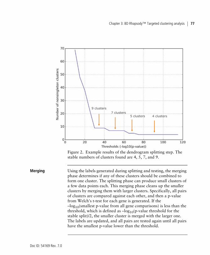
Starting from the top of the dendrogram, the tree is split into two candidate sub-trees under the constraint that the intra-cluster median correlation of the two sub-trees should be higher than the inter-cluster median correlation. The split is scored with the smallest p-value when performing Welch's t-tests for every gene. All possible splits are performed, and their scores are recorded. Various thresholds of –log10(p-value) cutoffs are attempted as the split criterion to generate multiple versions of the clustering results. A graph of number of clusters versus –log10(p-value) cutoff can be plotted to inspect the stable cut of the dendrogram (see Figure 2). A stable cut is defined as a plateau on the curve over a range of 5 on a log10-transformed p-value scale. Splitting results (sets of labels) corresponding to all stable cuts are kept and subjected to the next merging step.

Doc ID: 54169 Rev. 7.0


Figure 2. Example results of the dendrogram splitting step. The stable numbers of clusters found are 4, 5, 7, and 9.

Merging Using the labels generated during splitting and testing, the merging phase determines if any of these clusters should be combined to form one cluster. The splitting phase can produce small clusters of a few data points each. This merging phase cleans up the smaller clusters by merging them with larger clusters. Specifically, all pairs of clusters are compared against each other, and then a p-value from Welch's t-test for each gene is generated. If the –log10(smallest p-value from all gene comparisons) is less than the threshold, which is defined as –log10(p-value threshold for the stable split)/2, the smaller cluster is merged with the larger one. The labels are updated, and all pairs are tested again until all pairs have the smallest p-value lower than the threshold.

4 clusters5 clusters7 clusters

9 clusters

Doc ID: 54169 Rev. 7.0


Reporting the cluster assignment

Each cluster is denoted by an integer. Cells that cannot be merged with any other clusters (singletons) are given the label –1. The file, <sample_name>_<num_clusters>_Labels.csv, records the cluster assignment of each cell in the same order as in the loaded data table.

Reporting marker genes of each cluster

For each cluster, one-versus-rest tests are done using only the genes that have higher means in the cluster of interest. A table of important genes for each cluster is output as <sample_name>_<num_clusters>_Cluster_Features.csv along with additional information about each gene, including p-value, fold-change, and mean expression level within the cluster.

For each pair of clusters, Welch's t-test is performed to generate the gene list to differentiate two clusters the most. The list of results from all pairs is output as <sample_name>_<num_clusters>_Pairwise_Cluster_Features.csv.

To review clustering analysis metrics outputs, proceed to Reviewing clustering analysis output files (page 79).

Doc ID: 54169 Rev. 7.0


Reviewing clustering analysis output filesBefore you begin Obtain the output files after running clustering analysis on the

Seven Bridges Genomics platform or on a local installation. See the BD Single-Cell Genomics Analysis Setup User Guide (Doc ID: 47383).

Clustering analysis outputs

The BD Rhapsody Clustering Analysis app outputs one or more sets of four files (cluster labels, t-SNE projection labelled by cluster, cluster features, and pairwise cluster features) that describe levels of clustering:

Output File Content

t-SNE coordinates (page 80)

<sample_name>_bh-tSNEcoordinates.csv

Coordinates of the t-SNE projection

Cluster labels (page 82) <sample_name>_<num_clusters>_Labels.csv

Cluster membership per cell

t-SNE plot (page 83) <sample_name>_<num_clusters>_tSNE.png

Visualization of the t-SNE projection with cells colored by cluster labels

Over-represented genes in each cluster to all clusters (page 84)

<sample_name>_<num_clusters>_Cluster_Features.csv

Top 50 statistically over-represented genes compared to all clusters

Doc ID: 54169 Rev. 7.0


t-SNE coordinates File: <sample_name>_bh-tSNEcoordinates.csv

The output is the projection of the data using the t-SNE algorithm. See der Maaten and Hinton in References (page 70).The output file contains coordinates that you can use to generate other visualizations. The order of cells/rows listed in the output file is in the same order of cells/rows listed in the input file.

Over-represented genes in each cluster to every other cluster (page 85)

<sample_name>_<num_clusters>_Pairwise_Cluster_Features.csv

Top 50 statistically over-represented genes compared to every other cluster

(Optional) Concatenated data tables (page 86)

<sample names>_MolsPerCell.csv or <sample names>_Expression_Data.st

Combined data table; output only if multiple inputs specified

(Optional) Sample IDs (page 86)

SampleIDs.csv Table of sample IDs; output only if multiple inputs specified

Output (continued)

File Content

Doc ID: 54169 Rev. 7.0


For example:

Doc ID: 54169 Rev. 7.0


Cluster labels File: <sample_name>_<num_clusters>_Labels.csv

The output is the assignment of an integer representing the cluster label to each cell. The order of cells/rows listed in the output file is in the same order of cells/rows listed in the MolPerCell.csv input file. The value –1 means singletons, which are cells not assigned to any of the clusters. You can use this file and the coordinate file for additional clustering analysis.

For example:

Doc ID: 54169 Rev. 7.0


t-SNE plot File: <sample_name>_<num_clusters>_tSNE.png

The output is a visualization of the t-SNE plot with cells colored according to cluster label. The visualization shows the number of clusters that have been identified from the analysis.

Singletons are not associated with any cluster due to the low pair-wise correlation between the singleton and other cells in the sample. Singletons are infrequent.

For example:

Doc ID: 54169 Rev. 7.0


Over-represented genes in each cluster to all clusters

File: <sample_name>_<num_clusters>_Cluster_Features.csv

The output is a list of up to the top 50 statistically over-represented genes in each cluster as compared to all other clusters.

For example:

Metric Description

Cluster Identified cluster

Gene Over-expressed gene in this cluster compared to other clusters

p-Value This is –log10 of the p-value. The larger the value, the more significant the differential expression of the gene within the cluster.

Mean_of_Expression

Mean number of molecules in all cells in that cluster

Fold_Change_of_Expression

Fold change in mean expression of the gene in that cluster and all of the remaining cells

Doc ID: 54169 Rev. 7.0


Over-represented genes in each cluster to every other cluster

File: <sample_name>_<num_clusters>_Pairwise_Cluster_Features.csv

The output is a list of up to the top 50 statistically over-represented genes in each cluster as compared to every other cluster. The output shows the pairwise differential expression between all pairs of clusters:

Metric Description

Comparison The two clusters being compared

Gene Over-expressed gene in this cluster compared to the paired cluster

p-Value This is –log10 of the p-value. The larger the value, the more significant the differential level of the gene with the cluster.

Larger_Cluster The cluster with the higher mean expression level of the gene

Fold_Change_of_Expression_for_Larger_Cluster

Fold change of expression of the gene in that cluster and another cluster

Doc ID: 54169 Rev. 7.0


(Optional) Concatenated data tables

File: < sample names>_MolsPerCell.csv or <sample names>_Expression_Data.st

The output is a concatenated data table of all inputs (only if multiple data files are input).

(Optional) Sample IDs

File: SampleIDs.csv

The output is the Sample ID and the sample name associated with each molecule in the concatenated data file (only if multiple data files are input):

ReferencesClustering algorithm

Zhang JM, Fan J, Fan HC, Rosenfeld D, and Tse DN. An interpretable framework for clustering single-cell RNA-Seq datasets. BMC Bioinformatics. 2018;19:93–105. doi.org/10.1186/s12859-018-2092-7.

t-SNE van der Maaten LJP. Accelerating t-SNE using Tree-Based Algorithms. Journal of Machine Learning Research. 2014;15(Oct):3221–3245.

https://doi.org/10.1186/s12859-018-2092-7

https://doi.org/10.1186/s12859-018-2092-7

Doc ID: 54169 Rev. 7.0

Glossary

Doc ID: 54169 Rev. 7.0


B

BAM An alignment file in binary format. A binary SAM file.

C

CIGAR Compact Idiosyncratic Gapped Alignment Report. A sequence of base lengths to indicate base alignments, insertions, and deletions with respect to the reference sequence. See samtools.github.io/hts-specs/SAMv1.pdf.

CLS Cell label sequence.

D

DBEC Distribution-based error correction.

F

FASTA Text-based format that contains one or more DNA or RNA sequences.

FASTQ A file in standardized, text-based format that contains the output of read bases and per-base quality values from a sequencer.

L

L Common sequence.



Doc ID: 54169 Rev. 7.0

Chapter : Glossary 89

M

molecule A unique combination of a cell label, UMI sequence, and a gene. Without UMI adjustment methods, it is called raw molecule. With RSEC UMI adjustment, it is called RSEC-adjusted molecule. With additional DBEC UMI adjustment, it is called DBEC-adjusted molecule.

P

PhiX Control library used for sequencing runs.

R

R1 reads Contains information about the cell label and UMI.

R2 reads Contains information about the gene.

RSEC Recursive substitution error correction.

S

SAM Tab-delimited text file with sequence alignment data.

singlet A putative cell where more that 75% of sample tag reads are from a single tag.

singleton Clustering: Cell not assigned to any of the clusters. UMI correction/adjustment: Molecule that is represented by only one read.

Doc ID: 54169 Rev. 7.0


U

UMI Unique Molecular Identifier. A string of eight randomers immediately downstream of the cell label sequence (CLS) 3 of the R1 read that is used to uniquely label a molecule.

BD Single-Cell Genomics Bioinformatics Handbook

Documents

Transcript of BD Single-Cell Genomics Bioinformatics Handbook