bca 3 sem file

B.C.A III Semester

Software Laboratory III

Session 2014-15

SUPERVISION

Dr. Neeraj Dubey(Professor and Head, Dept. of Physics)

GUIDED BYMISS JAYA SONI

MR. PRAMOD SEN

Submitted ByName :MAHENDRA KUMAR PATEL

Enroll No: J/87401

Roll No. : 2162157

DEPARTMENT OF BCAContents:-

o Introduction to DBMS

o (SQL) Structure Query Language

o Data Structure using ‘C’

o Business Data Processing using

‘COBOL’

Database Management System [DBMS]

Database Management System or DBMS in short, refers to the technology of storing and retriving users data with utmost efficiency along with safety and security features. DBMS allows its users to create their own databases which are relevant with the nature of work they want. These databases are highly configurable and offers bunch of options.

Database is collection of data which is related by some aspect. Data is collection of facts and figures which can be processed to produce information. Name of a student, age, class and her subjects can be counted as data for recording purposes.

A database management system stores data, in such a way which is easier to retrieve, manipulate and helps to produce information.

Characteristics

Modern DBMS has the following characteristics:

Real-world entity: Modern DBMS are more realistic and uses real world entities to design its architecture. It uses the behavior and attributes too. For example, a school database may use student as entity and their age as their attribute.

Relation-based tables: DBMS allows entities and relations among them to form as tables. This eases the concept of data saving. A user can understand the architecture of database just by looking at table names etc.

Isolation of data and application: A database system is entirely different than its data. Where database is said to active entity, data is said to be passive one on which the database works and organizes. DBMS also stores metadata which is data about data, to ease its own process.

Less redundancy: DBMS follows rules of normalization, which splits a relation when any of its attributes is having redundancy in values. Following normalization, which itself is a mathematically rich and scientific process, make the entire database to contain as less redundancy as possible.

Consistency: DBMS always enjoy the state on consistency where the previous form of data storing applications like file processing does not guarantee this. Consistency is a state where every relation in database remains consistent. There exist methods and techniques, which can detect attempt of leaving database in inconsistent state.

Query Language: DBMS is equipped with query language, which makes it more efficient to retrieve and manipulate data. A user can apply as many and different filtering options, as he or she wants. Traditionally it was not possible where file-processing system was used.

ACID Properties: DBMS follows the concepts for ACID properties, which stands for Atomicity, Consistency, Isolation and Durability. These concepts are applied on transactions, which manipulate data in database. ACID properties maintains database in healthy state in multi-transactional environment and in case of failure.

Multiuser and Concurrent Access: DBMS support multi-user environment and allows them to access and manipulate data in parallel. Though there are restrictions on transactions when they attempt to handle same data item, but users are always unaware of them.

Multiple views: DBMS offers multiples views for different users. A user who is in sales department will have a different view of database than a person working in production department. This enables user to have a concentrate view of database according to their requirements.

Security: Features like multiple views offers security at some extent where users are unable to access data of other users and departments. DBMS offers methods to impose constraints while entering data into database and retrieving data at later stage. DBMS offers many different levels of security features, which enables multiple users to have different view with different features. For example, a user in sales department cannot see data of purchase department is one thing, additionally how much data of sales department he can see, can also be managed. Because DBMS is not saved on disk as traditional file system it is very hard for a thief to break the code

Data model tells how the logical structure of a database is modeled. Data Models are fundamental entities to introduce abstraction in DBMS. Data models define how data is connected to each other and how it will be processed and stored inside the system.

Entity-Relationship Model

Entity-Relationship model is based on the notion of real world entities and relationship among them. While formulating real-world scenario into database model, ER Model creates entity set, relationship set, general attributes and constraints.

ER Model is best used for the conceptual design of database.

ER Model is based on:

Entities and their attributes

Relationships among entities

These concepts are explained below.

[Image: ER Model]

Entity

An entity in ER Model is real world entity, which has some properties called attributes. Every attribute is defined by its set of values, called domain.

For example, in a school database, a student is considered as an entity. Student has various attributes like name, age and class etc.

Relationship

The logical association among entities is called relationship. Relationships are mapped with entities in various ways. Mapping cardinalities define the number of association between two entities.

Mapping cardinalities:

o one to one

o one to many

o many to one

o many to many

ER-Model is explained here.

Relational Model

The most popular data model in DBMS is Relational Model. It is more scientific model then others. This model is based on first-order predicate logic and defines table as an n-ary relation.

[Image: Table in relational Model]

The main highlights of this model are:

Data is stored in tables called relations.

Relations can be normalized.

In normalized relations, values saved are atomic values.

Each row in relation contains unique value

Each column in relation contains values from a same domain.

Relational Model is explained here.

http://www.tutorialspoint.com/dbms/relation_data_model.htm

http://www.tutorialspoint.com/dbms/er_model_basic_concepts.htm

The design of a Database Management System highly depends on its architecture. It can be centralized or decentralized or hierarchical. DBMS architecture can be seen as single tier or multi tier. n-tier architecture divides the whole system into related but independent n modules, which can be independently modified, altered, changed or replaced.

In 1-tier architecture, DBMS is the only entity where user directly sits on DBMS and uses it. Any changes done here will directly be done on DBMS itself. It does not provide handy tools for end users and preferably database designer and programmers use single tier architecture.

If the architecture of DBMS is 2-tier then must have some application, which uses the DBMS. Programmers use 2-tier architecture where they access DBMS by means of application. Here application tier is entirely independent of database in term of operation, design and programming.

3-tier architecture

Most widely used architecture is 3-tier architecture. 3-tier architecture separates it tier from each other on basis of users. It is described as follows:

[Image: 3-tier DBMS architecture]

Database (Data) Tier: At this tier, only database resides. Database along with its query processing languages sits in layer-3 of 3-tier architecture. It also contains all relations and their constraints.

Application (Middle) Tier: At this tier the application server and program, which access database, resides. For a user this application tier works as abstracted view of database. Users are unaware of any existence of database beyond application. For database-tier, application tier is the user of it. Database tier is not aware of any other user beyond application tier. This tier works as mediator between the two.

User (Presentation) Tier: An end user sits on this tier. From a users aspect this tier is everything. He/she doesn't know about any existence or form of database beyond this layer. At this layer multiple views of database can be provided by the application. All views are generated by applications, which resides in application tier.

Multiple tier database architecture is highly modifiable as almost all its components are independent and can be changed independently.

NormalizationIf a database design is not perfect it may contain anomalies, which are like a bad dream for database itself. Managing a database with anomalies is next to impossible.

Update anomalies: if data items are scattered and are not linked to each other properly, then there may be instances when we try to update one data item that has copies of it scattered at several places, few instances of it get updated properly while few are left with there old values. This leaves database in an inconsistent state.

Deletion anomalies: we tried to delete a record, but parts of it left undeleted because of unawareness, the data is also saved somewhere else.

Insert anomalies: we tried to insert data in a record that does not exist at all.

Normalization is a method to remove all these anomalies and bring database to consistent state and free from any kinds of anomalies.

First Normal Form:

This is defined in the definition of relations (tables) itself. This rule defines that all the attributes in a relation must have atomic domains. Values in atomic domain are indivisible units.

[Image: Unorganized relation]

We re-arrange the relation (table) as below, to convert it to First Normal Form

[Image: Relation in 1NF]

Each attribute must contain only single value from its pre-defined domain.

Second Normal Form:

Before we learn about second normal form, we need to understand the following:

Prime attribute: an attribute, which is part of prime-key, is prime attribute.

Non-prime attribute: an attribute, which is not a part of prime-key, is said to be a non-prime attribute.

Second normal form says, that every non-prime attribute should be fully functionally dependent on prime key attribute. That is, if X → A holds, then there should not be any proper subset Y of X, for that Y → A also holds.

[Image: Relation not in 2NF]

We see here in Student_Project relation that the prime key attributes are Stu_ID and Proj_ID. According to the rule, non-key attributes, i.e. Stu_Name and Proj_Name must be dependent upon both and not on any of the prime key attribute individually. But we find that Stu_Name can be identified by Stu_ID and Proj_Name can be identified by Proj_ID independently. This is called partial dependency, which is not allowed in Second Normal Form.


We broke the relation in two as depicted in the above picture. So there exists no partial dependency.

Third Normal Form:

For a relation to be in Third Normal Form, it must be in Second Normal form and the following must satisfy:

No non-prime attribute is transitively dependent on prime key attribute

For any non-trivial functional dependency, X → A, then either

X is a superkey or,

A is prime attribute.

[Image: Relation not in 3NF]

We find that in above depicted Student_detail relation, Stu_ID is key and only prime key attribute. We find that City can be identified by Stu_ID as well as Zip itself. Neither Zip is a superkey nor City is a prime attribute. Additionally, Stu_ID → Zip → City, so there exists transitive dependency.


We broke the relation as above depicted two relations to bring it into 3NF.

Boyce-Codd Normal Form:

BCNF is an extension of Third Normal Form in strict way. BCNF states that

For any non-trivial functional dependency, X → A, then X must be a super-key.

In the above depicted picture, Stu_ID is super-key in Student_Detail relation and Zip is super-key in ZipCodes relation. So,

Stu_ID → Stu_Name, Zip

And

Zip → City

Confirms, that both relations are in BCNF.

(SQL)

STURCTURE QUERY LANGUAGE

SQL(Structure Query language)Table of Contents

1. Introduction To SQL1.1 Data Definition Language1.2 Data Manipulation Language

2.Introduction To SQL Server2.1 SQL Server Management Studio2.2 Create a new Database 2.3 Queries

3. CREATE TABLE3.1 Database Modeling3.2 Create Tables using the Designer Tools3.3 SQL Constraints

3.4 FOREIGN KEY3.5 NOT NULL/Required Columns3.6 UNIQUE3.7 CHECK3.8 DEFAULT

4.INSERT INTO5.UPDATE

1.Introduction To SQL

SQL (Structured Query Language) is a database computer language designed

For managing data in relation database management system (RDMS).

SQL, is a standardized computer language that was originally developed by IBM for querying, altering and defining relational databases, using declarative Statements.

What can SQL do?

SQL can execute queries against a database. SQL can insert records in a database. SQL can update record in a database. SQL can delete from a database. SQL can create new database.

There are lots of different database system ,or DBMS(DataBase Management System) such as;

Microsoft SQL server. Oracle. Microsoft access. IBM DB2. …Lots of other systems

1.1 Data Definition LanguageThe Data Definition Language (DDl) manage table and index structure. The most basic item of DDL likes as; CREATE, ALTER, RENAME and DROP statement.

CREATE an object (a table, for example) in the database. DROP deletes an object in database. ALTER modifies the structure an existing from various ways-

for adding a columns to an existing table.

1.2Data Manipulation Language

The Data Manipulation Language is the subset of SQL used to add, delete, update data.

Operation SQL Description

CREATE INSERT INTO Insert new data item into a database

READ SELECT Extract data from database

UPDATE UPDATE Update data in a database

DELETE DELETE Delete data from database

1.3Introduction To SQL Server

Microsoft is vendor of SQL server. The newest version is “SQL server 2012”.We can download different editions of SQL server and used. SQL server consists of Database Engine a Management studio. The database engine has no graphical engine- it is just a server running in the background running of your computer (preferable on the server).the management studio is graphical tool for configuration view the information in the database. It can be installed on the server or on the client (or both).

2.1 SQL Server Management Studio

SQL Server Management Studio is a GUI tools included with SQl server Configuration, managing and administering all component within Microsoft SQL server .The tool include both scripts editor or graphical tool that work with objects and features of the server. As mentioned earlier, version of SQL Server Management Studio is also available for SQL Server Express Edition, for which It is known as SQL Server Management Studio Express A central feature of SQL Server Management Studio is the Object

Explorer,which allows the user to browse, select, and act upon any of the objects within the server.

2.2 Create a new Database

It is quite simple to create a new database in Microsoft SQL Server. Just right-- click on the “Databases” node and select “New‐ Database…”

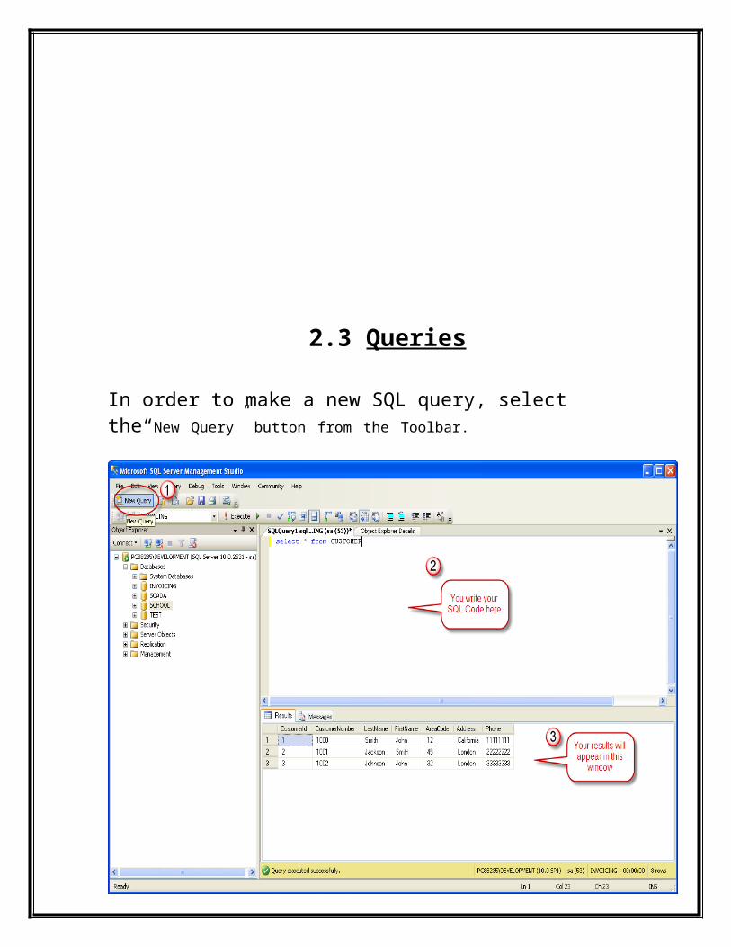
2.3 Queries

In order to make a new SQL query, select the“New Query” button from the Toolbar.

Here we can write any kind of queries that is supported by the SQL language.

1. CREATE TABLE

Before you start implementing your tables In the database, you

should always spend sometime design your tables properly using a

design tool like, e.g., Erwin, Toad Data Modeler Power Desiger, Visio, etc. This is called Database Modeling. The CREATE TABL:E statement is used to create a table in a database.

CREATE TABLE table name(column_name1 data type,column_name2 data_type,column_name3 data_type,....)

3.1 Database Modeling

As mention in the beginning of the chapter, you should always start with databaseModeling before you start implementing the tables in a database system. BelowWe see a database model in created with ERwin.

With this tool we can transfer the database model as tables into different database systems, such as SQL Server. Data Modeler Community Edition is free with a 25 objects limit. It has support for Oracle, SQL Server, My SQL, ODBC and Sybase. 3.2 Create Tables using the Designer Tools

Even if you can do “everything” using the SQL language, it is sometimes easier toDo it in the designer tools in the Management Studio in SQL Server.

Instead of Creating a script you may as well easily use the designer for creating tables.Step1: Select “New Table …”:

Step2: Next, the table designer pops up where you can add columns, data types,Etc.

In this designer we may also specify Column Names, Data Types, etc.Step 3: Save the table by clicking the Save button.

3.3 SQL Constraints

Constraints are used to limit the type of data that can go into a table. ConstraintsCan be specified when a table is created (with the CREATE TABLE statement) or after the table is created of data that can go into a table. (with the ALTER TABLE statement). Here are the most important constraintsPRIMARY KEYNOT NULLUNIQUEFOREIGN KEY

CHECKDEFAULT IDENTITYIn the sections below we will explain some of these in detail.

3.4 FOREIGN KEY

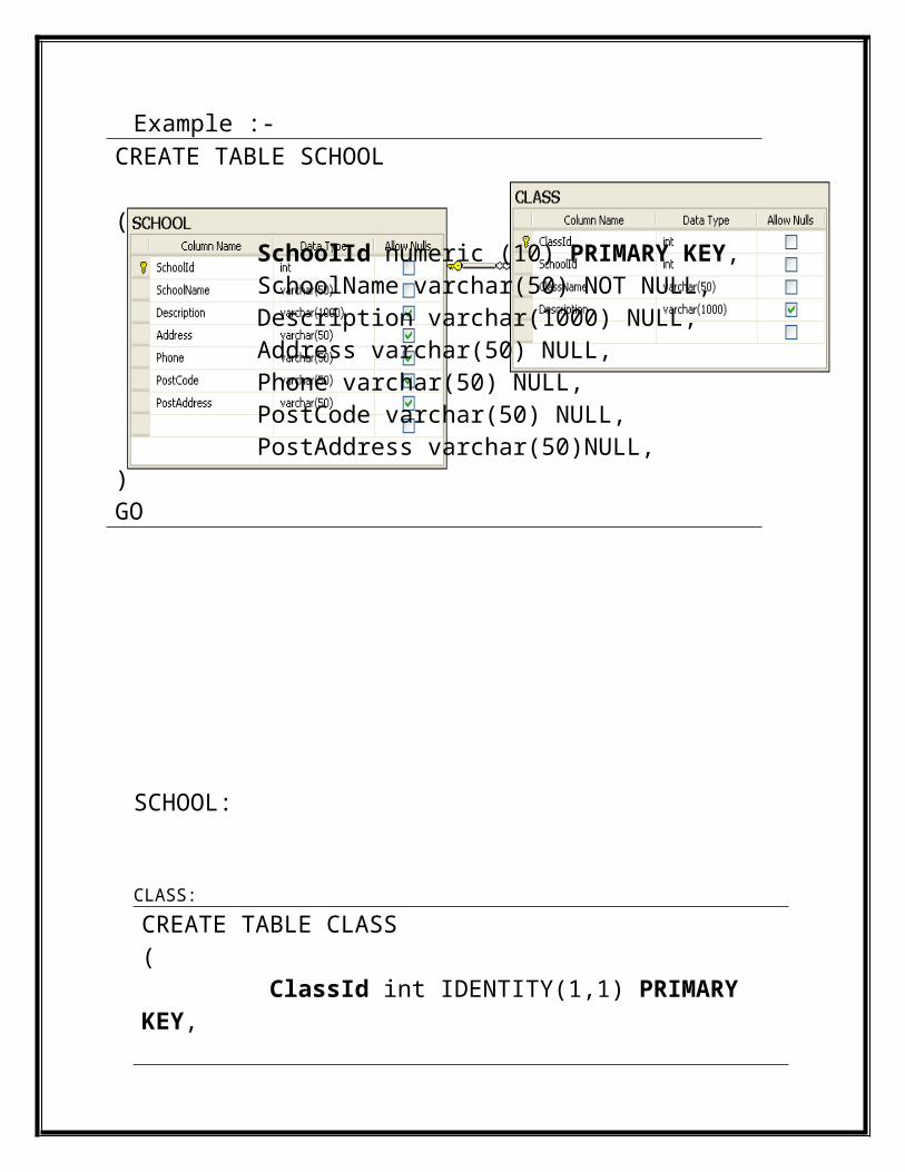
A FOREIGN KEY in one table points to a PRIMARY KEY in another table.Example :-

CREATE TABLE SCHOOL

( SchoolId numeric (10) PRIMARY KEY, SchoolName varchar(50) NOT NULL, Description varchar(1000) NULL, Address varchar(50) NULL, Phone varchar(50) NULL, PostCode varchar(50) NULL, PostAddress varchar(50)NULL,)GO

SCHOOL:

CLASS:

CREATE TABLE CLASS( ClassId int IDENTITY(1,1) PRIMARY KEY, SchoolId int NOT NULL FOREIGN KEY REFERENCES SCHOOL (SchoolId), ClassName varchar(50) NOT NULL UNIQUE, Description varchar(1000) NULL,)GO

3.5 NOT NULL/Required Columns

The NOT NULL constraint enforces a column to NOT accept NULL values.The NOT NULL constraint enforces a field to always contain a value.This means that you cannot insert a new record, or update a record without adding a value to this field.

CREATE TABLE [CUSTOMER]( CustomerId int IDENTITY(1,1) PRIMARY KEY, CustomerNumber int NOT NULL UNIQUE, LastName varchar(50) NOT NULL, FirstName varchar(50) NOT NULL, AreaCode int NULL, Address varchar(50) NULL, Phone varchar(50) NULL,)GO

If we take a closer look at the CUSTOMER table created earlier:

Setting NULL/NOT NULL in the Designer Tools: In the Table Designer you can easily set which columns that should allow NULL or not:

4.INSERT INTO

The INSERT INTO statement is used to insert a new row in a table. It is possible to write the INSERT INTO statement in two forms. The first form doesn't specify the column names where the data will be inserted, Only their values:

INSERT INTO table_nameVALUES (value1, value2, value3,...)

Example:This form is recommended!INSERT INTO CUSTOMER (CustomerNumber,LastName, FirstName, AreaCode,Address, Phone)VALUES ('1000', 'Smith', 'John', 12, 'California', '11111111')

Example :

5.UPDATE

The UPDATE statement is used to update existing records in a table.

The syntax is as follows:

UPDATE table_nameSET column1=value, column2=value2,...WHERE some_column=some_value

PRACTICAL NO. 1

Create Table for Student Information Like Name, age add, Place

Class etc. Using Create Table Command.

Syntax :- Create table name (column name data type size).

Sql > create table student.

(

Name char (10),

Age Numeric (3),

Add. Archer (30),

Phone no. (10),

Class Archer (5),

DOB date time,

);

TABLE NAME STUDENT:-

NAME AGE ADDRESS PHONE CLASS DOBRizban 19 Snah nagar 98564554565 B.C.A 14-11-1996Praveen 20 Civil line 98654795665 B.C.A 07-05-1995Ram 19 Gopalganj 98657512365 B.C.A. 11-06-1996PRACTICAL NO. 2

Insert data into tables using both types of insert command.

Syntax :-

Sql >_ insert into table name values (1,2,…………….)

Sql >_ insert into student value (“Rizban”, ”19”, “snah nagar”,

“98567895665”, “B.C.A.”, “12/02/1994”)

TABLE NAME STUDENT :-

NAME AGE ADDRESS PHONE CLASS DOBRizban 19 Snah nagar 98567895665 B.C.A. 12/02/1994

TYPE Syntax :- _ insert table name (column name 1,2 ………. ) Sql > insert student (name. age ) value (Rizban , 19)


NAME AGE

Rizban 19

PRACTICAL NO. 3

Add another column into data base using alert command.

Syntax :- sql> alter table name add/modify/drop column name

Add a column:- sql > alter table student add present varchar(s).


NAME AGE ADDRESS PHONE CLASS DOB %

Rizban 19 Snehanagar 9858655856 B.C.A 10/02/1994 82

Praveen 20 Civil line 9745656335 B.C.A. 11/05/1995 86

Ram 19 Gopalguanj 9826564231 B.C.A. 12/06/1993 84


NAME ADDRESS PHONE CLASS DOB %

Rizban Snehanagar 9858655856 B.C.A 10/02/1994 82

Praveen Civil line 9745656335 B.C.A. 11/05/1995 86

Ram Gopalguanj 9826564231 B.C.A. 12/06/1993 84

Modify a column :- sql>alter table student modify (present varchar (31));


NAME AGE ADDRESS PHONE CLASS DOB %

Rizban 19 Snehanagar 9858655856 B.C.A 10/02/1994 82

Praveen 20 Civil line 9745656335 B.C.A. 11/05/1995 86

Ram 19 Gopalguanj 9826564231 B.C.A. 12/06/1993 84

PRECTICAL NO.4

Select particular type of data using select command using, like Function e.t.c.

1. SELECT COMMAND :-

we can see of select data from database by of this command.

Syntax:- sql>select *from student ;

Student:-

NAME AGE ADDRESS PHONE CLASS DOB

Rizban 19 Snehanagar 8103659856 B.Com 14/02/1994

Praveen 20 Civil line 9657854566 B.Com 06/05/1995

Ram 19 Gopalguanj 9175956575 B.Com 21/06/1993

Bunty 19 Manorama 9987484566 B.Com 12/05/1998

Bablu 22 sadar 9748796789 B.Com 10/12/1994


2. LIKE:- We can use of this command see the same any value.

Syntax :-sql>*from student where name like “s%”

STUDENT


ram 19 Gopalganj 8475956596 B.Com 25/06/1993


5 BETWEEN:-we can use of this command see the data of it’s specify range.

Syntax:- sql>select * from student where age between 17+19

STUDENT :-



ram 19 Gopalganj 8475956596 B.Com 25/06/1993


PRACTICAL NO. 5

Update particular type of data using update command.

UPDATE :- Update Command are used to update the value of Field.

Syntax:-

Sql>update table name set column name = value

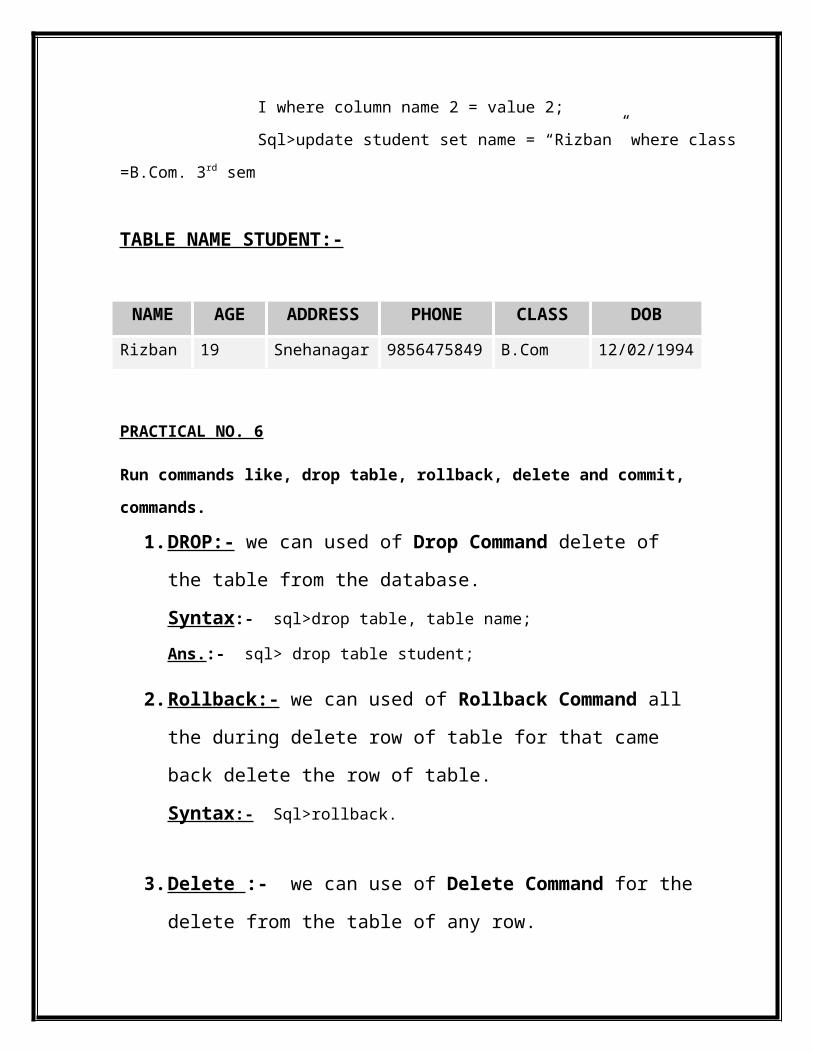
I where column name 2 = value 2;

Sql>update student set name = “Rizban” where class =B.Com. 3rd sem




PRACTICAL NO. 6

Run commands like, drop table, rollback, delete and commit, commands.

1. DROP:- we can used of Drop Command delete of the table

from the database.

Syntax:- sql>drop table, table name;

Ans.:- sql> drop table student;

2. Rollback:- we can used of Rollback Command all the during

delete row of table for that came back delete the row of table.

Syntax :- Sql>rollback.

3. Delete :- we can use of Delete Command for the delete from

the table of any row.

Syntax:-

a) sql>delete form student.

b) Sql>delete from student where name =”Rajesh”.

4. Commit command :- we can use of Commit Command in the

last or after every session.

Syntax :- Sql>commite;

PRACTICAL NO. 7

Arrange columns data item in ascending or descending order.

Order by:-

Order by commands used to ascending of descending

Order in column value.

Syntax:-

sql>select * from student order by column name desc.




Praveen 20 Makroniya 9652124596 B.Com 15/05/1995

DATA STRUCTURE USING ‘C’

History Of ‘C’ Language‘C’ seems a strange name for a programming. But this strange sounding language is one of the most popular computer languages today because it is a structured, high-level, machine independent language. It allow software develop program without worrying about the hardware platforms where they will be implemented.

The root of all modern language is ALGOL, introduced in the early 1960s. ALGOL was the first computer language to use a block structure.Although it never becomes popular in USA, it was widely used in Europe. ALGOL gave the concept of structured programming to the computer science community.

In 1967, Martin Richards developed a language called BCPL (Basic combined programming language) primarily for waiting system software. In 1970, Ken Thompson created a language using many feature of BCPL and called it simply B.B was used to create early version of UNIX operating system at bell Laboratories Both BCPL and B were “typeless” system programming languages.

For many years, C was used mainly in academic environments, but eventually with the release the of many C compilers for commercial use and the increasing popularity of UNIX, it began to gain widespread support among computer professionals. Today C is running under a variety of operating system and hardware platform.

During 1970s, C had evolved into what is now as “traditional C”. the language become more popular after publication of the book ‘The c programming language’ by brain kerning ham and Dennis Ritchie in 1978. the book was so popular that the language came to be know as “k&R C” among the programming community. The rapid that development of different version of the language that were similar but often incompatible. This posted a serious problem for system developers.

All popular computer language are dynamic in nature. The continue to improve their power and scope by incorporation new feature and C is no exception.

Introduction Of ‘C’ Language

A programming language us designed to help certain kinds of data consisting of a numbers, character and string and to provide useful output know as information. The task of processing of data is accomplished by executing a sequence of precise instruction called a program. These introductions are formed using certain symbol and word according to some rigid rules knows as system rules (or grammar). Every program introduction must confirm precisely to the syntax rules of the language.

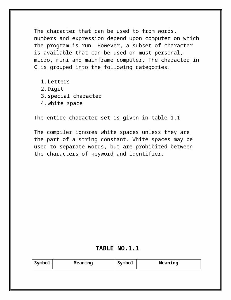
Character Set

The character that can be used to from words, numbers and expression depend upon computer on which the program is run. However, a subset of character is available that can be used on must personal, micro, mini and mainframe computer. The character in C is grouped into the following categories.

1. Letters 2. Digit 3. special character 4. white space

The entire character set is given in table 1.1

The compiler ignores white spaces unless they are the part of a string constant. White spaces may be used to separate words, but are prohibited between the characters of keyword and identifier.

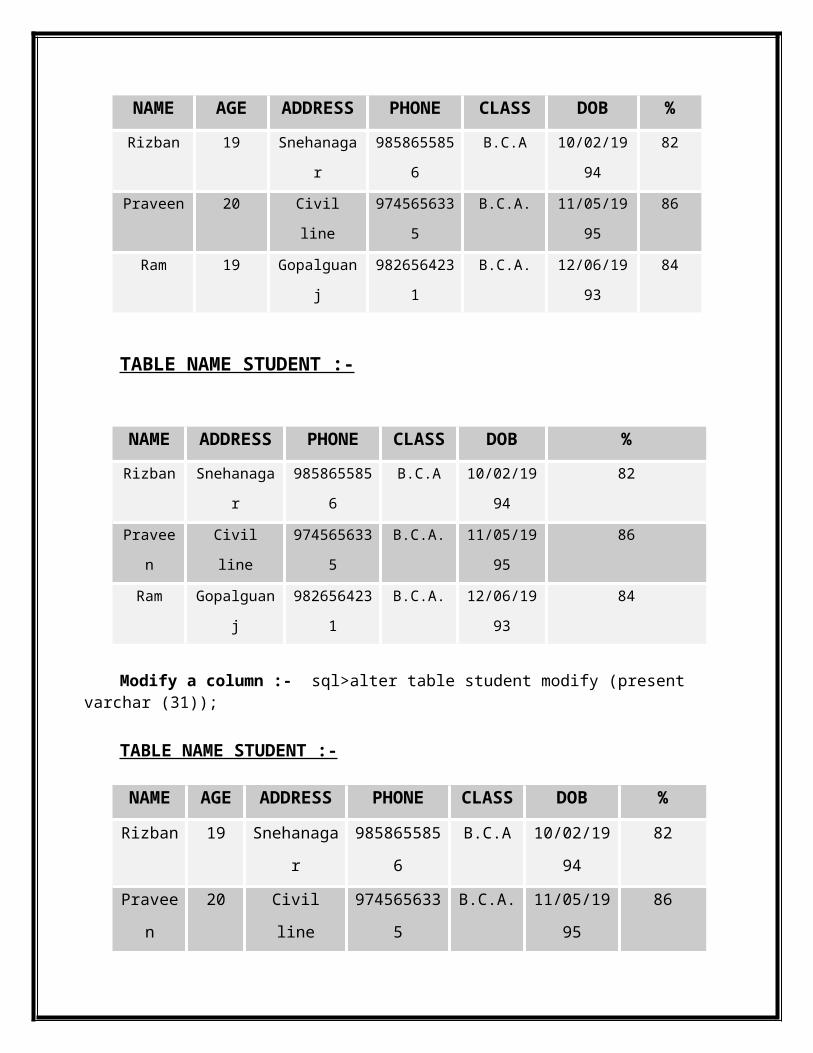
TABLE NO.1.1

Symbol Meaning Symbol Meaning

,

;

?

“

(

[

{

<

/

I

+

#

-

&

=

Comma

Semicolon

Question Mark

Double quote mark

Left Parenthesis’

Left bracket

Left brace

Left angle bracket

Slash(forward)

Vertical bar

Plus sign

Pound sign

Underscore

Ampersand

Equal sign

.

:

!

‘

)

]

}

>

\

~

_

%

^

*

<>

Period

Colon

Exclamation marks

Single quite mark

Right parenthesis

Right bracket

Right brace

Right angle bracket

Backslash

Tilde

Minus sign

Percent sign

Caret

Asterisk

Also used as greater than

and less than

Fig:-1.1

Basic structure of C Program

The example discussed so far illustrate that a C program can be viewed as a group of building blocks called function. A function is subroutine that may include one more statement designed to perform a specific task. To write a C program, we first create function and then together. A C program may containOne or more section as show in fig:-1.2

Fig:-1.2

Documentation section

Link section

Definition section

Global declaration section

Main function

{ Declaration part Execution part }

Subprogram section

Function 1Function 2

-Function n

In regards to: User define function

Simple Program

Consider a very simple program given in fig 1.3

main { /*……printing begins…...…*/ printf (“welcome to C”); /*……printing ends………..*/}

S

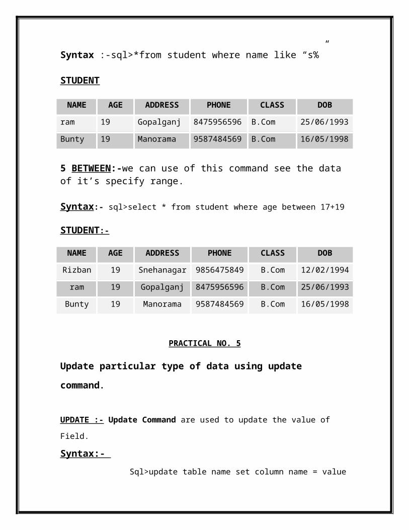
Fig 1.3

Program: Program for Array implementation of Stack.

#include<stdio.h>#include<conio.h>#define maxstack5struck stack //***********STACK DECLARATION IS C *************//{

int item [raxstack];int top;

};void push (struct stack *ps, int x);int pop (struct stack *ps);vodi display (struct stack * ps);int isempty (struct stack * ps);int isfull (struct stack * ps);void main (){struct stack s;int choice x;s.tep - -1;clrscr();do{printf(“\n1>push \n2->pop\n3-> display\/4->exit”);sprintf(“\n enter your choice->”);scanf (“%d”,&choice);switch(choice)

{case 1: printf(“enter the element for push”);scanf(“%d”,&x);push(&s,x);brack;case 2: x = pop (&s);if(x!=-9999);printf(“\n popped value =%d”,x);getch();break;case 3: display (&s);getch();brack();}

}

while(choice!=4);}void push(struct stack * ps, int x){

if(isful(ps)){

printf(“stack over flow”);return;

}ps - > top =ps-> top+1;ps - > item [ps->top]=x;

}int pop(struck stack * ps)

{int x;if(isempty(ps)){printf(“stack is under flow”);return(-9999)}

x=ps->item[ps->top];ps->top = ps->top-1;return;}

void display(struct stack * ps){int I;if(isempty(ps))

{printf(“\n stack is empty”);return;}

for (i=0;i<=ps->top;i++)printf(“\t%d”,ps->item[i]);}int isempty (struct stack * ps) { if(ps->top = = -1) return (1); else return(0); }int isful(struct stack * ps) { if(ps->tip = = maxtask-1)return(1);else

return(0);}

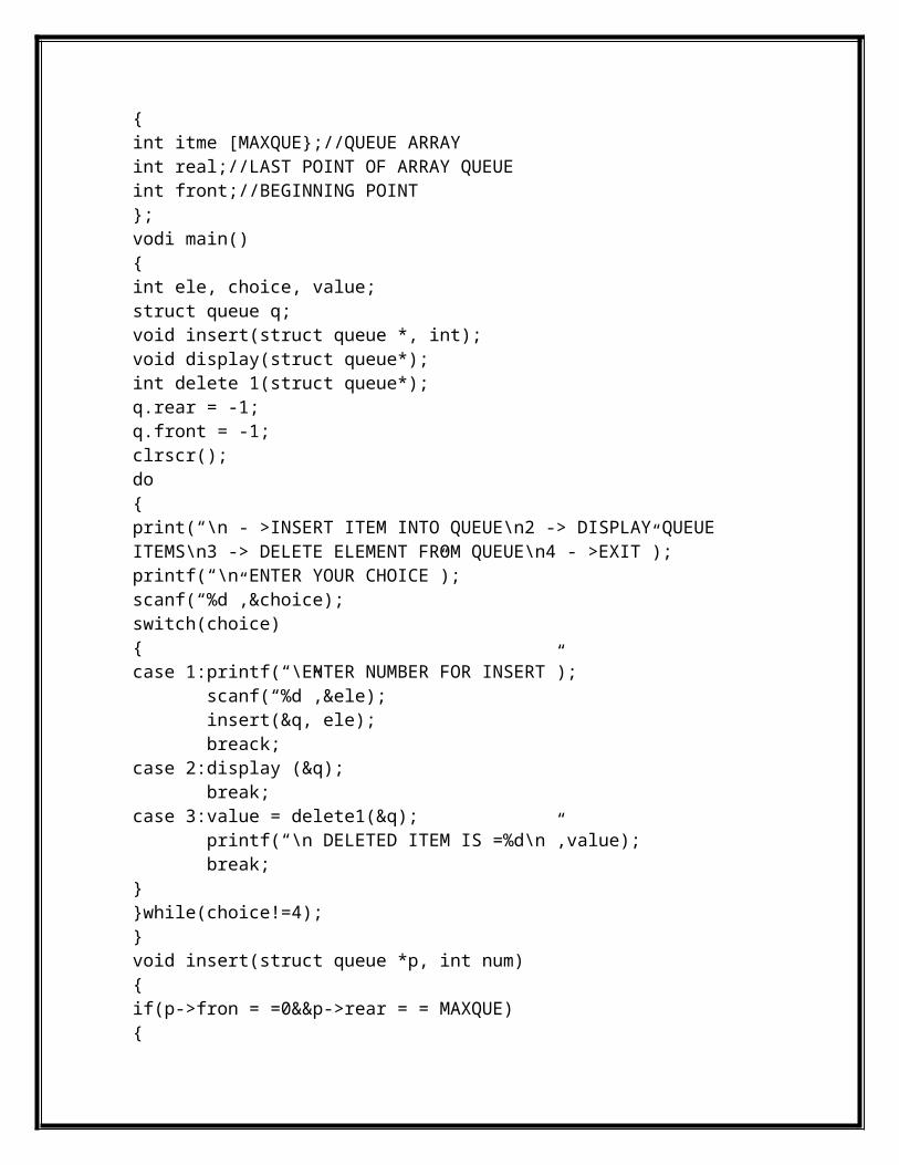
Program: Program for implementation of Queue using Array.

#include<conio.h>#includ.h#define MAXQUE5Struct queue {int itme [MAXQUE};//QUEUE ARRAYint real;//LAST POINT OF ARRAY QUEUEint front;//BEGINNING POINT};vodi main(){int ele, choice, value;struct queue q;void insert(struct queue *, int);void display(struct queue*);int delete 1(struct queue*);q.rear = -1;q.front = -1;clrscr();do{print(“\n - >INSERT ITEM INTO QUEUE\n2 -> DISPLAY QUEUE ITEMS\n3 -> DELETE ELEMENT FROM QUEUE\n4 - >EXIT”);printf(“\n ENTER YOUR CHOICE”);scanf(“%d”,&choice);switch(choice){case 1:printf(“\ENTER NUMBER FOR INSERT”); scanf(“%d”,&ele); insert(&q, ele); breack;case 2:display (&q); break;case 3:value = delete1(&q); printf(“\n DELETED ITEM IS =%d\n”,value); break;}}while(choice!=4);}void insert(struct queue *p, int num){if(p->fron = =0&&p->rear = = MAXQUE){

printf(“\n nohhh!!!!!!!!!! QUEUE IS OVERFLOW”);}{p->rear =p->rear +1;p->itme[p->rear]=num;if(p->front = = -1)return;}}void display(struct queue *p){int I;if(p->rear = =-1&&p->front = =-1){printf(“\noffffoooooo!!!!!!!! QUEUE IS ENPTY”);return;}elsefor(i=p->front;i<=p->reat;i++)printf(“%d”,p->item[i])}int delet1(struct queue *p){int ele ;if(p->front = =-1){printf(“\n QUEUE IS UNDER FLOW”);return;}elseele=p->item[p->front];if(p->front = =p->rear){p->front=-1;p->rear=-1;}else{p->front=p->front+1;}return(ele)}

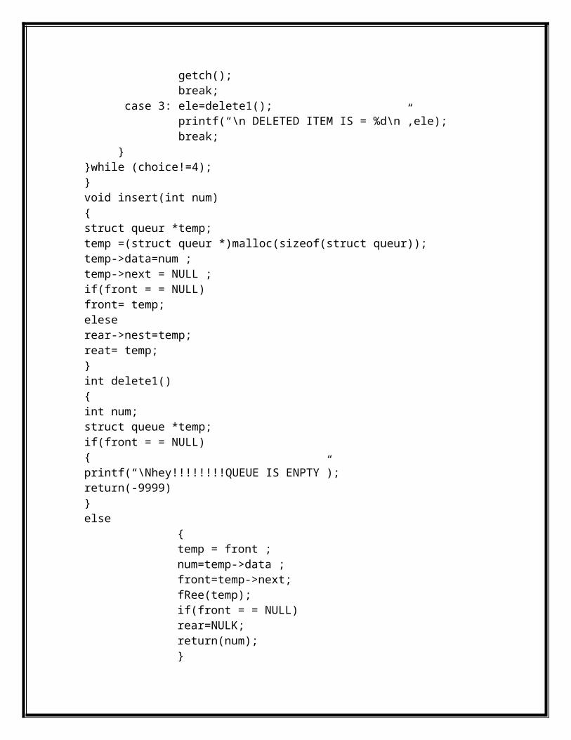
Program: Program for performing various operations over queue using linked list.

#include<conio.h>#include<stdio.h>struct queue{ int data; struct queue *next;};struct queue *rear, *front;void main();{ int choice, ele; void insert(int);int delete1();void display();rear = NULL;front =NULL;do{print(“\n -> INSERT ITEM INTO QUEUE\n2->DISPLAY QUEUE iTEMS\n3-> DELETE ELEMENT FROM QUEUE\n4->EXIT”);printf(“%d”,&choice);switch(choice) { case 1: printf(“\n ENTER NUMBER FOR INSERT”); scanf(“%d”,&ele); insert(ele) break; case 2: display(); getch(); break; case 3: ele=delete1(); printf(“\n DELETED ITEM IS = %d\n”,ele); break; }}while (choice!=4);}void insert(int num){struct queur *temp;temp =(struct queur *)malloc(sizeof(struct queur));temp->data=num ;temp->next = NULL ;if(front = = NULL)front= temp;

eleserear->nest=temp;reat= temp;}int delete1(){int num;struct queue *temp;if(front = = NULL){printf(“\Nhey!!!!!!!!QUEUE IS ENPTY”);return(-9999)}else

{temp = front ;num=temp->data ;front=temp->next;fRee(temp);if(front = = NULL)rear=NULK;return(num);}

}void display (){struct queue * temp;temp = front;if(front = = NULL&&rear = = NULL){printf(“OHOOOOOO QUEUE IS EMPTY”);}while(tem! = NULL){printf(“%d\t”, temp-> data);temp = temp-next;}}

Program: Program for linked list implementation of stack.

#include<conio.h>#include<stdio.h>#include<stdlib.h>struct queue

{ int data;// ITEM sturct ink *next;//ADDRESS OF NEXT ELEMENT

}; sTRUCT LINT *TOP;//TOP IS THE LAST ELEMENTvoid main(){

int choice,ele;void push(int);int pop();void display();clrscr();top =NULL;do{

printf(“\n1->PUSH\n2->POP\n3->DISPLAY\n4->EXIT\Nenter your choice->”);

scanf(“%d”,&choice);switch(choice){

case 1 :printf(“ENTER THE NUMBER WHICH YOU WANT TO INSERT”);

scanf(“%d”,ele);push(ele);case 2 :ele = pop();if(ele!=-9999)printf(“\n POPED ELEMENT IS =%d,ele”);break;case 3 :display();getch();break;}

}while(choice!=4);}void push (int num){ struct link *stemp; temp=(struct lint*)malloc(sizeof(struct link)); temp->data=num; temp->next=top; top=temp;}

int pop() { struct link *temp; int ele; if (top = = NULL)

{printf(“STACK IS EMPITY”);return(-9999)}

else temp=top; ele=temp->data; top=top->next; free(temp); return(ele); }{struct link *temp;if(top==NULL) { printf(“\n STACK IS EMPITY”); return; }elsetemp=top;while(temp!=NULL) { printf(“%d”, temp=>data); temp=temp->next; }}

Program: Program to search an element using liner search

technique.

#include<conio.h>#include<stdio.h>void main(){ int a[100],n, i, item, loc=-1; clrscr(); printf(“\n Enter the number of element:”); scanf(“%d”,&n); printf(“Enter the numbers:\n”); for(i=0, i<=n-1; i++){ scanf(“%d”,&a[i]);}printf(“\n enter the number to be searched:”);scanf(“%d”,&itam);for(i=0; i<n-1; i++){ if(item==a[i]) { loc=i; break; }}if (loc>=0)printf(“\n%d is found is position%d”, item, loc+1);elseprintf(“\n item does not exist”);getch();}

Program: Program to search an element for list of element using binary search technique.

#include<conio.h>#include<stdio.h>void main(){ int a[100], i, loc, mid, beg, ent, n, flag=0, item; clrscr(); printf(“HOW MANY ELEMENT”); scanf(“%d”,&n); printf(“ENTER THE ELEMENT OF ARRAY\n”); for(i=0; i<=n-1; i++) { scanf(“%d”,&a[i];) } printf(“Enter the element to be search\n”); scanf(“%d”,&itme); loc=0; beg=0; ent=n-1; while((beg<=end) && (item !=a[mid])) { mid=((beg+end)/2) if(item==a[mid]) {

printf(“Search is successful\n”)’loc = mid;printf(“positin of the item %d\n”, loc+1);flag=flag+1;

} else if (item < a[mid]) end=mid=1; else beg=mid+1; }if(flag==0){ printf(“search is not successfull\n”);}getch();}

Program: Program for TOWER OF HANOI using recursion.

#include<conio.h>#include<stdio.h>

void transfer(int n, char from, char to, char temp);/* function prototype*/main (){ int n; printf(“Welcome to the TOWERS OF HANOI \n\n”); printf(“How many disk?”); scanf(“%d”,&n); printf(“\n”); transfer (n, ‘L’, ‘R’, ‘C’);}void transfer (int n, char from, char to, char temp)/* transfer n disks from one pole to another*//* n = number of disks fron = origin to = destination temp = temporary storage */{ if(n>0) {

/* move n-1 disks fron their origin to the temporary*/ transfer(n-1fron, temp, to);/* move nth disk from its origin to its destination*/print(“move disk %d from %c\n, n, from,to”);/* move the n-1 disks from the temporary to destination transfer(n-1, temp, to, from);

} return;}

PROGRAMMING

IN ‘COBOL’

History of ‘COBOL’ Language

In the 1950s there was a growing need for high-level programming language Suitable for business data processing, to meet this demand the united states Department of Defense convinced a conference on the 28th and 29th may 1958, which was attended by users from civil and government organization, computer manufacturers and other interested group. Out of this conference three group were formed for the actual design of the language.

The short team committee, having modified there earlier report, submit a final report in December of the same year. The report was accept and then published in April 1960.

On May 5, 1961, COBOL-61 WAS published with some revision of the first accepts report and this provided the basic for letter versions. The users stared writing COBOL programs when the first COBOL compiler becomes available in early 1965. But it was only in August 1968 that a standard version of the language was approved by the American national standard institute (ANSI). This version knows as ANSI-68 COBOL or COBOL-68 is the first official standard of COBOL. The next revised/official standard was introduced in 1974 and is knows as ANSI-68 COBOL or COBOL-74 (The official name is American National standard COBOL x 3:23 - 1974).this version is currently implement in almost every machine.

Coding seat of ‘COBOL’1-6 7 8-11 12-72 73-80

Sequence (s) Indicator (I) Area AOr (A)

Margins A

Area BOr (B)

Margins B

Identification (I)

Page no.(1-3)

Serial no.(4-6)

*/

(both for non-

executable statement)

-(For

continuation)

Division/section/

paragraph

All executable statement

Remarks

Positive Field 1-6 Sequence 7 Indicator 8-11 Area A/Margin A12-7 Area B/Margin B72-80 Identification

Q:-1. Welcome Program?

IDENTIFICATION DIVISION. PROGRAM– ID. HELLO. ENVIROMENT DIVISION. DATA DIVISION.PROCEDURE DIVISION. MAIN()DISPLAY “HELLO!” DISPLAY “WELCOME TO THE WORLD OF COBOL:”STOP RUN.

Output:-

HELLOWELCOM TO THE WORLD OF COBOL.

Q:-2. Write a program for add a two number?

IDENTIFICATION DIVISION.PROGRAM-ID.ENVIRONMENT DIVISION.DATA DIVISION.WORKING-STORAGE SECTION.77 A PIC 9977 B PIC 9977 C PIC 999PROCEDURE DIVISION.MAIN()DISPLAY ”Enter first number ”. ACCEPT A.DISPLAY ”Enter second number ”. ACCEPT B.ADD A,B GIVING C.DISPLAY ”Answer is” C. STOP RUN.

Output:-

Enter first number A=5Enter second number B=6ADD=A+BA+B=CAnswer is C=11

Q:-3. Write a program for substraction of two number?

IDENTIFICATION DIVISION.PROGRAM-ID.ENVIRONMENT DIVISION.DATA DIVISION.WORKING-STORAGE SECTION.77 A PIC 9977 B PIC 9977 C PIC 999PROCEDURE DIVISION.MAIN()DISPLAY ”Enter first number ”. ACCEPT A.DISPLAY ”Enter second number ”. ACCEPT B.SUB A FROM B GIVING C.DISPLAY ”Answer is” C. STOP RUN.

Output:-

Enter first number A=5Enter second number B=3SUB=A-BA-B=CAnswer is C=2

Q:-4. Write a program for multiplication of two number?

IDENTIFICATION DIVISION.PROGRAM-ID.ENVIRONMENT DIVISION.DATA DIVISION.WORKING-STORAGE SECTION.77 A PIC 9977 B PIC 9977 C PIC 999PROCEDURE DIVISION.MAIN()DISPLAY ”Enter A ”. ACCEPT A.DISPLAY ”Enter B ”. ACCEPT B.MUL A BY B GIVING C.DISPLAY ”Answer is” C. STOP RUN.

Output:-

Enter A=6Enter B=3MUL=A*BA*B=CAnswer is C=18

Q:-5. Write a program for division of two number?

IDENTIFICATION DIVISION.PROGRAM-ID.ENVIRONMENT DIVISION.DATA DIVISION.WORKING-STORAGE SECTION.77 A PIC 9977 B PIC 9977 C PIC 9977 D PIC 99PROCEDURE DIVISION.MAIN()DISPLAY ”Enter A ”. ACCEPT A.DISPLAY ”Enter B ”. ACCEPT B.DIVIDE A BY B GIVING C REMAINDER D.DISPLAY ”Answer is” C. DISPLAY ”Remainder is” D. STOP RUN.

Q:-6. Write a program for find the greatest number?

IDENTIFICATION DIVISION.PROGRAM-ID.ENVIRONMENT DIVISION.DATA DIVISION.WORKING-STORAGE SECTION.77 A PIC 99977 B PIC 999PROCEDURE DIVISION.MAIN()DISPLAY ”Enter A ”. ACCEPT A.DISPLAY ”Enter B ”. ACCEPT B.IF A>B.DISPLAY ”Greater number is ” A. ELSE.DISPLAY ”Greater number is ” B.STOP RUN.

Output:-

Enter A3Enter B4 Greater Number is 4

Q:-7. Write a program for find the percentage?

IDENTIFICATION DIVISION.PROGRAM-ID.ENVIRONMENT DIVISION.DATA DIVISION.WORKING-STORAGE SECTION.77 PER PIC 99V99PROCEDURE DIVISION.MAIN()DISPLAY ”Enter Percentage”.ACCEPT PER.IF PER>60 OR PER=60.DISPLAY ”First Division”. IF PER <60 AND (PER NOT <45).DISPLAY ”Second Division”. IF PER<45 AND PER>33.DISPLAY ”Third Division ”.STOP RUN.

Q:-8. Write a program to calculate Simple Interest?

IDENTIFICATION DIVISION.PROGRAM-ID.ENVIRONMENT DIVISION.DATA DIVISION.WORKING-STORAGE SECTION.77 P PIC 9977 T PIC 9977 R PIC 9977 SI PIC 9999.99PROCEDURE DIVISION.MAIN()DISPLAY ”Enter P value”.ACCEPT P.DISPLAY ”Enter T value”.ACCEPT T.DISPLAY ”Enter R value”.ACCEPT R.DISPLAY ”Principle amount=” , P.DISPLAY ”Number of time=” , T.DISPLAY ”Rate of Interest=” , R.COMPUTE SI=(P*T*R)/100.DISPLAY ”Simple Interest=” , SI.STOP RUN.

Output:-

ENTER P:5000ENTER T:5ENTER R:3PROCESSING ………..SINPLE INTEREST 0075.00

Q:-9. Write a program for multiplication table in COBOL?

IDENTIFICATION DIVISION.PROGRAM-ID.ENVIRONMENT DIVISION.DATA DIVISION.WORKING-STORAGE SECTION.77 A PIC 9977 B PIC 99 VALUE 077 C PIC 99PROCEDURE DIVISION.MAIN()DISPLAY ”Enter the number for multiplication table=” , A.ACCEPT A.PERFORM UNTIL B=10.MULTIPLY A BY B GIVING C.DISPLAY A ”*” B ”=” C.ADD 1 TO B.END-PERFORM.STOP RUN.

Output:-

5*1=55*2=105*3=155*4=205*5=255*6=305*7=355*8=405*9=455*10=50

Q:-10. Write the program sign condition?

IDENTIFICATION DIVISION.PROGRAM-ID. S-CONDITION.ENVIRONMENT DIVISION.DATA DIVISION.WORKING-STORAGE SECTION.

77 A PIC S999.PROCEDURE DIVISION.MAIN.DISPLAY “ENTER ANY NO.”ACCEPT AIF A IS POSITIVE. DISPLAY”A >0 + VE”.IF IS A NIGATIVE. DISPLAY “A<0 – VE”.IF A IS ZERO DISPLAY “A =0”.STOP RUN.

Output:-

ENTER ANY NO:-27A<0 -VE

Output:-

ENTER ANY NO:18A>0 +VE

bca 3 sem file

Documents

Transcript of bca 3 sem file