bayhan gur crowncom2017 - boun.edu.tr
168
1 TUTORIAL Maching Learning for Spectrum Sharing in Wireless Networks Sept. 21, 2017, 10:45 - 12:30 Lisbon, Portugal Suzan Bayhan (TU Berlin, [email protected]) Gurkan Gur (Bogazici University, [email protected])
Transcript of bayhan gur crowncom2017 - boun.edu.tr
1
TUTORIAL
Maching Learning for Spectrum Sharing in Wireless Networks
Sept. 21, 2017, 10:45 - 12:30
Lisbon, Portugal
Suzan Bayhan (TU Berlin, [email protected]) Gurkan Gur (Bogazici University, [email protected])
/170
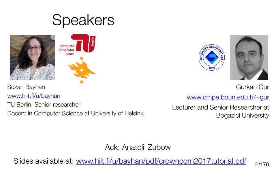
Speakers
Suzan Bayhan www.hiit.fi/u/bayhan TU Berlin, Senior researcher Docent in Computer Science at University of Helsinki
2
Gurkan Gur www.cmpe.boun.edu.tr/~gur
Lecturer and Senior Researcher at Bogazici University
Ack: Anatolij ZubowSlides available at: www.hiit.fi/u/bayhan/pdf/crowncom2017tutorial.pdf
/170
Outline
3
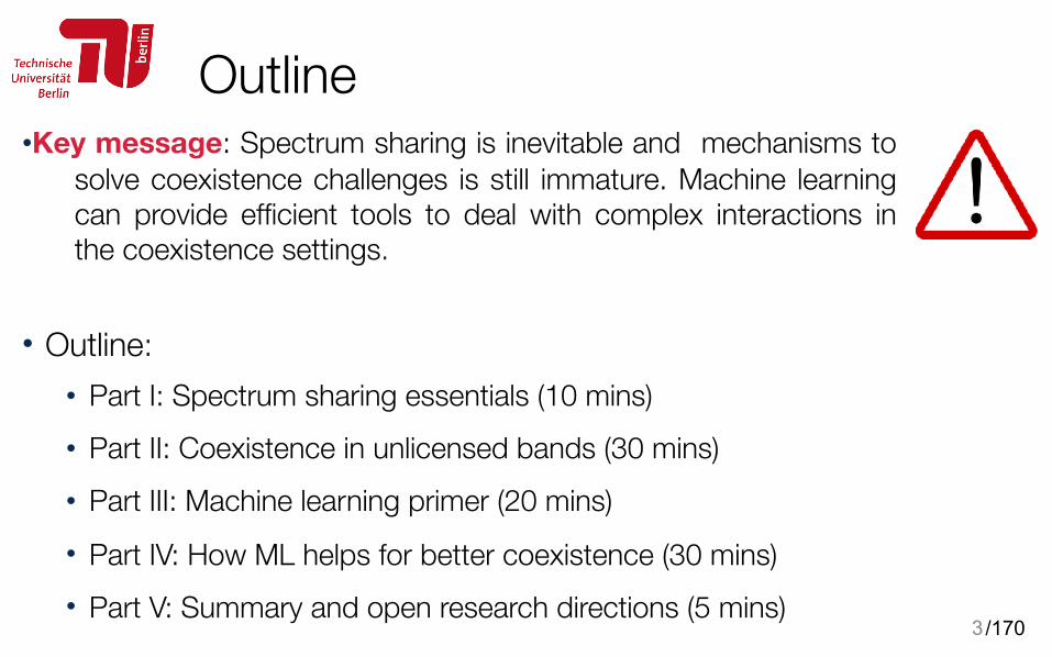
•Key message: Spectrum sharing is inevitable and mechanisms to solve coexistence challenges is still immature. Machine learning can provide efficient tools to deal with complex interactions in the coexistence settings.
• Outline:
• Part I: Spectrum sharing essentials (10 mins) • Part II: Coexistence in unlicensed bands (30 mins) • Part III: Machine learning primer (20 mins) • Part IV: How ML helps for better coexistence (30 mins) • Part V: Summary and open research directions (5 mins)
/1704
Part I Spectrum Sharing in Wireless Networks
• Why to share the spectrum? • Modes of sharing • Challenges in harmonious coexistence • Current solutions for coexistence in
wireless networks
10
/170
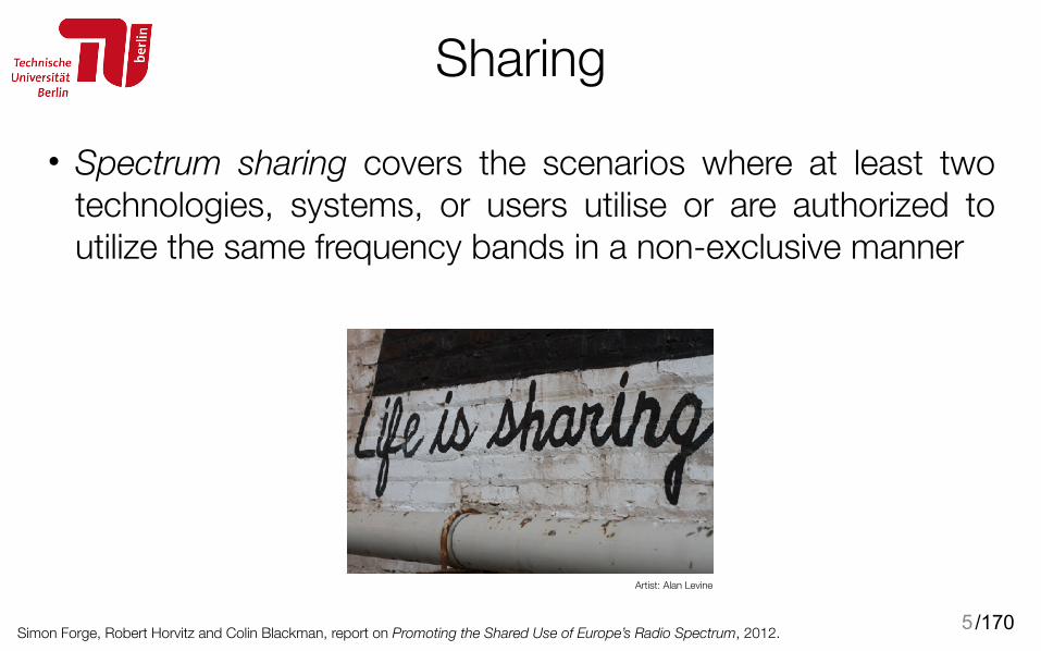
• Spectrum sharing covers the scenarios where at least two technologies, systems, or users utilise or are authorized to utilize the same frequency bands in a non-exclusive manner
5
Sharing
Simon Forge, Robert Horvitz and Colin Blackman, report on Promoting the Shared Use of Europe’s Radio Spectrum, 2012.
Artist: Alan Levine
/170
Networks are getting denser
6
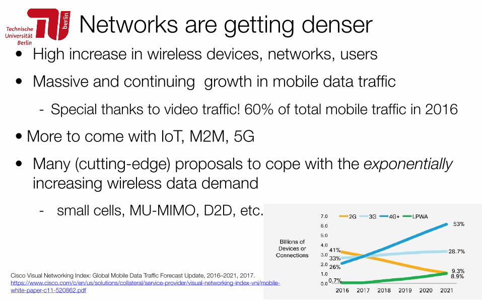
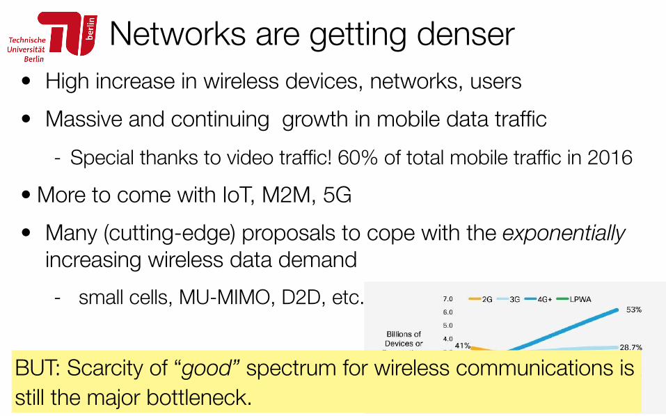
• High increase in wireless devices, networks, users • Massive and continuing growth in mobile data traffic
- Special thanks to video traffic! 60% of total mobile traffic in 2016 • More to come with IoT, M2M, 5G • Many (cutting-edge) proposals to cope with the exponentially
increasing wireless data demand - small cells, MU-MIMO, D2D, etc.
Cisco Visual Networking Index: Global Mobile Data Traffic Forecast Update, 2016–2021, 2017.https://www.cisco.com/c/en/us/solutions/collateral/service-provider/visual-networking-index-vni/mobile-white-paper-c11-520862.pdf
/170
Networks are getting denser
7
• High increase in wireless devices, networks, users • Massive and continuing growth in mobile data traffic
- Special thanks to video traffic! 60% of total mobile traffic in 2016 • More to come with IoT, M2M, 5G • Many (cutting-edge) proposals to cope with the exponentially
increasing wireless data demand - small cells, MU-MIMO, D2D, etc.
Cisco Visual Networking Index: Global Mobile Data Traffic Forecast Update, 2016–2021, 2017.https://www.cisco.com/c/en/us/solutions/collateral/service-provider/visual-networking-index-vni/mobile-white-paper-c11-520862.pdf
BUT: Scarcity of “good” spectrum for wireless communications is still the major bottleneck.
/170
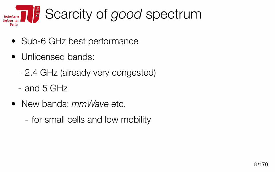
Scarcity of good spectrum
8
• Sub-6 GHz best performance • Unlicensed bands:
- 2.4 GHz (already very congested) - and 5 GHz
• New bands: mmWave etc. - for small cells and low mobility
/170
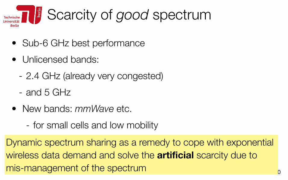
Scarcity of good spectrum
9
• Sub-6 GHz best performance • Unlicensed bands:
- 2.4 GHz (already very congested) - and 5 GHz
• New bands: mmWave etc. - for small cells and low mobility
Dynamic spectrum sharing as a remedy to cope with exponential wireless data demand and solve the artificial scarcity due to mis-management of the spectrum
/170
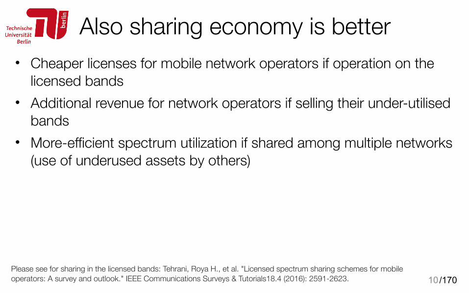
Also sharing economy is better• Cheaper licenses for mobile network operators if operation on the
licensed bands • Additional revenue for network operators if selling their under-utilised
bands • More-efficient spectrum utilization if shared among multiple networks
(use of underused assets by others)
10Please see for sharing in the licensed bands: Tehrani, Roya H., et al. "Licensed spectrum sharing schemes for mobile operators: A survey and outlook." IEEE Communications Surveys & Tutorials18.4 (2016): 2591-2623.
/170
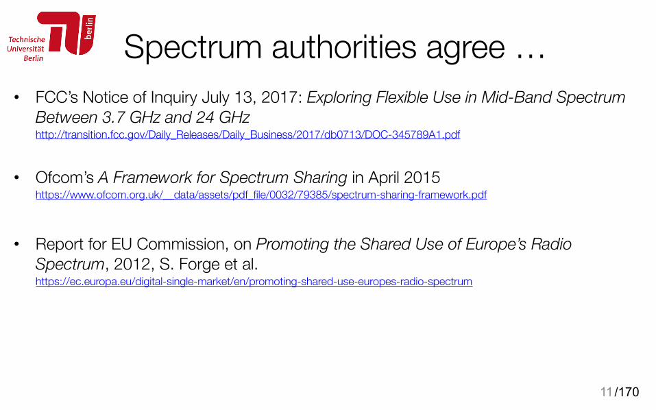
Spectrum authorities agree …• FCC’s Notice of Inquiry July 13, 2017: Exploring Flexible Use in Mid-Band Spectrum
Between 3.7 GHz and 24 GHz http://transition.fcc.gov/Daily_Releases/Daily_Business/2017/db0713/DOC-345789A1.pdf
• Ofcom’s A Framework for Spectrum Sharing in April 2015 https://www.ofcom.org.uk/__data/assets/pdf_file/0032/79385/spectrum-sharing-framework.pdf
• Report for EU Commission, on Promoting the Shared Use of Europe’s Radio Spectrum, 2012, S. Forge et al. https://ec.europa.eu/digital-single-market/en/promoting-shared-use-europes-radio-spectrum
11
/170
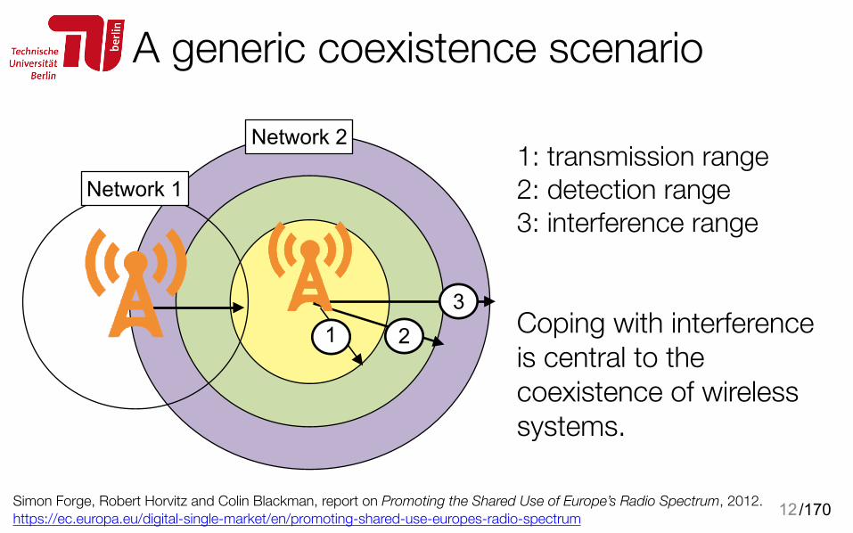
A generic coexistence scenario
12
Coping with interference is central to the coexistence of wireless systems.
1: transmission range 2: detection range 3: interference range
Simon Forge, Robert Horvitz and Colin Blackman, report on Promoting the Shared Use of Europe’s Radio Spectrum, 2012.https://ec.europa.eu/digital-single-market/en/promoting-shared-use-europes-radio-spectrum
23
Network 1
Network 2
1
/170
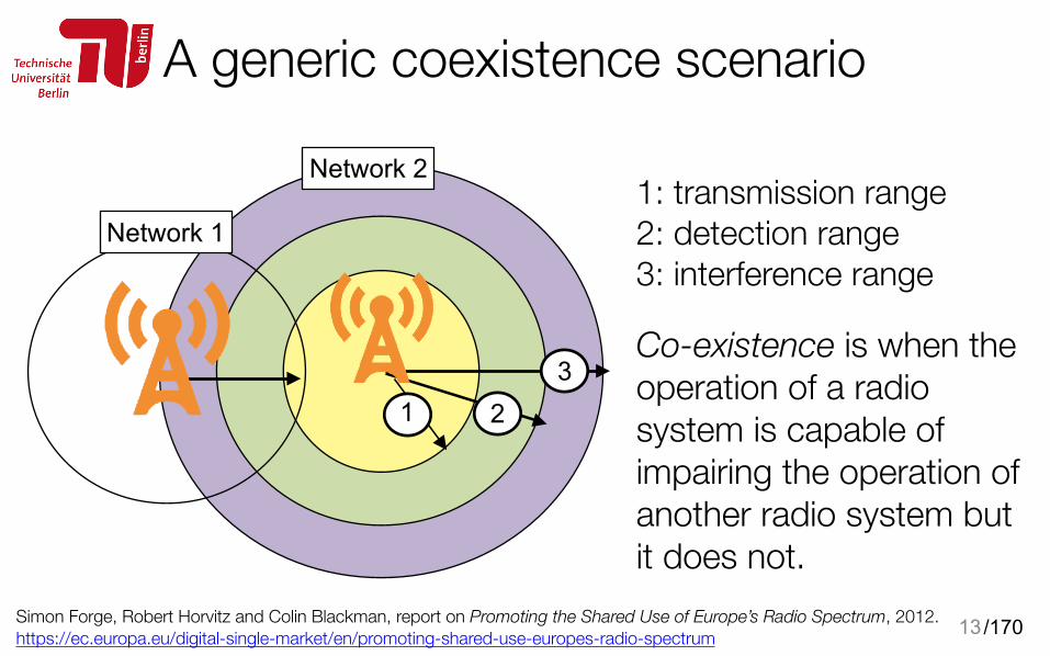
A generic coexistence scenario
13
Co-existence is when the operation of a radio system is capable of impairing the operation of another radio system but it does not.
1: transmission range 2: detection range 3: interference range
Simon Forge, Robert Horvitz and Colin Blackman, report on Promoting the Shared Use of Europe’s Radio Spectrum, 2012.https://ec.europa.eu/digital-single-market/en/promoting-shared-use-europes-radio-spectrum
23
Network 1
Network 2
1
/170
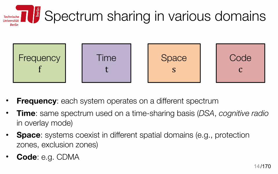
Spectrum sharing in various domains
• Frequency: each system operates on a different spectrum • Time: same spectrum used on a time-sharing basis (DSA, cognitive radio
in overlay mode) • Space: systems coexist in different spatial domains (e.g., protection
zones, exclusion zones) • Code: e.g. CDMA
14
Frequency f
Time t
Space s
Code c
/170
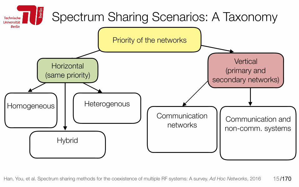
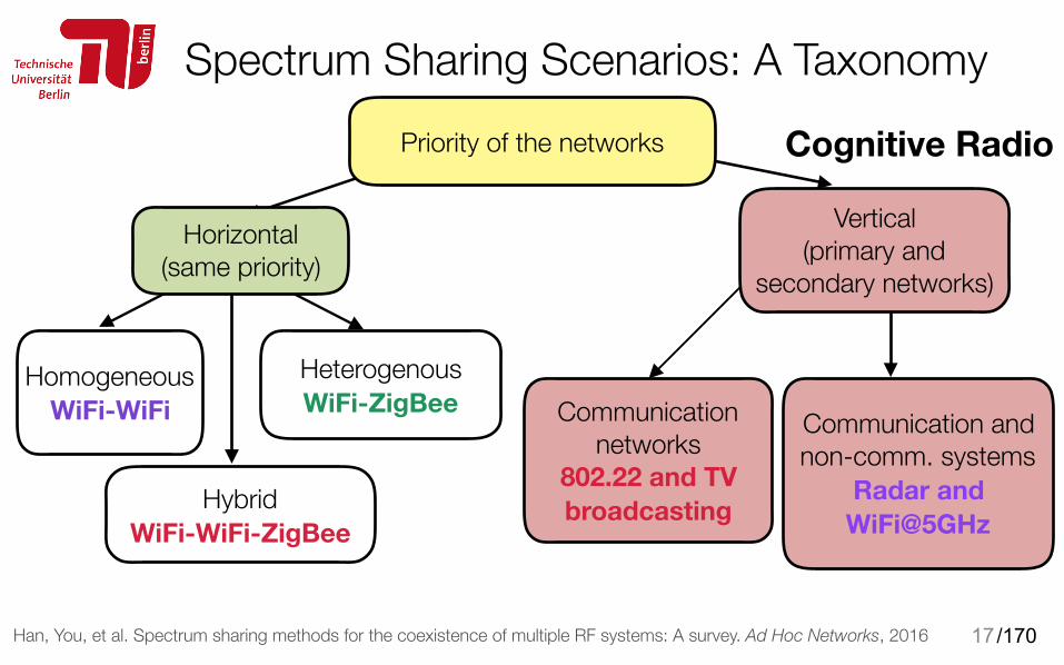
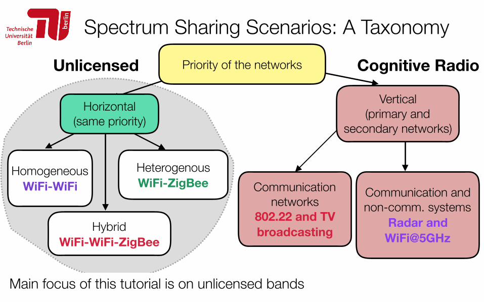
Spectrum Sharing Scenarios: A Taxonomy
15
Priority of the networks
Homogeneous Heterogenous
Hybrid WiFi-WiFi-ZigBee
Communication networks
802.22 and TV broadcasting
Communication and non-comm. systems
Radar and WiFi@5GHz
Vertical (primary and
secondary networks)
Han, You, et al. Spectrum sharing methods for the coexistence of multiple RF systems: A survey. Ad Hoc Networks, 2016
Horizontal (same priority)
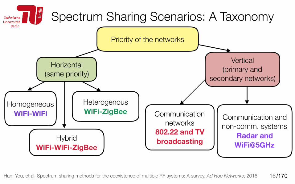
/170
Spectrum Sharing Scenarios: A Taxonomy
16
Priority of the networks
Communication networks
802.22 and TV broadcasting
Communication and non-comm. systems
Radar and WiFi@5GHz
Han, You, et al. Spectrum sharing methods for the coexistence of multiple RF systems: A survey. Ad Hoc Networks, 2016
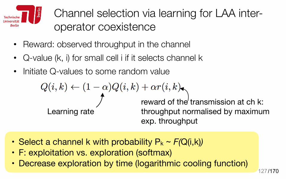
Homogeneous WiFi-WiFi
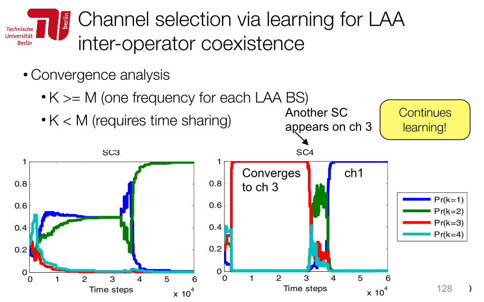
Heterogenous WiFi-ZigBee
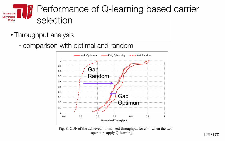
Hybrid WiFi-WiFi-ZigBee
Horizontal (same priority)
Vertical (primary and
secondary networks)
/17017
Priority of the networks
Homogeneous WiFi-WiFi
Heterogenous WiFi-ZigBee
Hybrid WiFi-WiFi-ZigBee
Communication networks
802.22 and TV broadcasting
Communication and non-comm. systems
Radar and WiFi@5GHz
Cognitive Radio
Spectrum Sharing Scenarios: A Taxonomy
Han, You, et al. Spectrum sharing methods for the coexistence of multiple RF systems: A survey. Ad Hoc Networks, 2016
Horizontal (same priority)
Vertical (primary and
secondary networks)
/170
Spectrum Sharing Scenarios: A Taxonomy
18
Priority of the networks
Homogeneous WiFi-WiFi
Heterogenous WiFi-ZigBee
Hybrid WiFi-WiFi-ZigBee
Communication networks
802.22 and TV broadcasting
Communication and non-comm. systems
Radar and WiFi@5GHz
Cognitive RadioUnlicensed
Main focus of this tutorial is on unlicensed bands
Horizontal (same priority)
Vertical (primary and
secondary networks)
/170
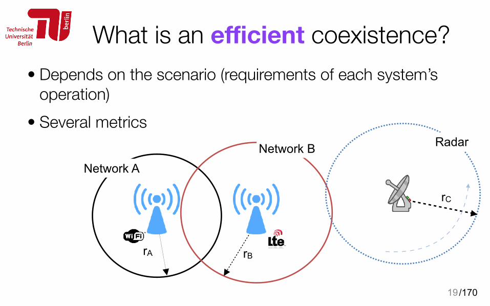
What is an efficient coexistence?• Depends on the scenario (requirements of each system’s
operation) • Several metrics
19
Network ANetwork B
rBrA
Radar
rC
/170
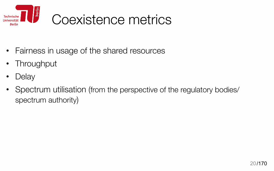
Coexistence metrics
• Fairness in usage of the shared resources • Throughput • Delay • Spectrum utilisation (from the perspective of the regulatory bodies/
spectrum authority)
20
/170
Main challenges in wireless coexistence
21
Challenge #1 Heterogeneity
(other challenges are also mostly due to heterogeneity)
/170
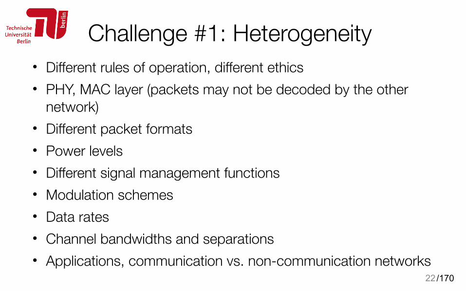
Challenge #1: Heterogeneity• Different rules of operation, different ethics • PHY, MAC layer (packets may not be decoded by the other
network) • Different packet formats • Power levels • Different signal management functions • Modulation schemes • Data rates • Channel bandwidths and separations • Applications, communication vs. non-communication networks
22
/170
Main challenges in wireless coexistence
23
Challenge #2 Power asymmetry
/170
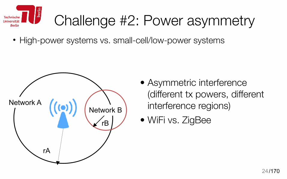
Challenge #2: Power asymmetry• High-power systems vs. small-cell/low-power systems
24
Network A
rB
rA
Network B
• Asymmetric interference (different tx powers, different interference regions)
• WiFi vs. ZigBee
/170
Main challenges in wireless coexistence
25
Challenge #3 Lack of communication among
co-existing networks
/170
Challenge #3: lack of communication
• Networks controlled by different operators • Networks using different technologies • No well-defined means for negotiation, e.g., residential WLANs
26
/170
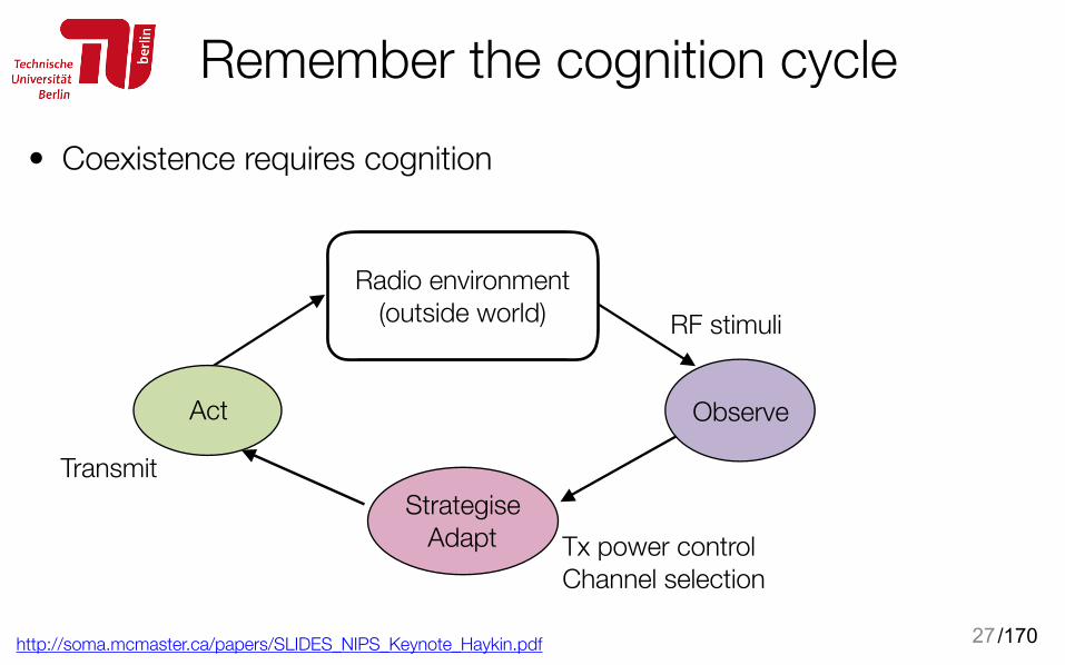
Remember the cognition cycle
http://soma.mcmaster.ca/papers/SLIDES_NIPS_Keynote_Haykin.pdf 27
Tx power control Channel selection
Radio environment (outside world) RF stimuli
Observe
Strategise Adapt
Act
Transmit
• Coexistence requires cognition
/170
Some coexistence guidelines • IEEE 802.19 Wireless Coexistence Technical Advisory Group (TAG)
within the IEEE 802 LAN/MAN Standards Committee: coexistence between unlicensed wireless networks • 802.19.1: Coexistence in TV bands
• IEEE 802.15 Task Group 2: Recommended Practice on Coexistence of IEEE 802.11 and Bluetooth
• P802.22b amendment: Self-coexistence protocol for 802.22 networks: Coexistence Beacon Protocol (CBP)
• P 1932.1: Standard for Licensed/Unlicensed Spectrum Interoperability in Wireless Mobile Networks
28
/170
Summary of Part I• Sharing is vital for meeting the demand for wireless capacity • Coexistence is the main challenge in shared spectrum access • Heterogeneity of networks pose substantial difficulties • Metrics and requirements still not totally agreed upon
29
/170
Further Reading for Part I • Han, You, et al. "Spectrum sharing methods for the coexistence of multiple RF
systems: A survey." Ad Hoc Networks 53 (2016): 53-78. • Beltran, Fernando et al "Understanding the current operation and future roles of
wireless networks: Co-existence, competition and co-operation in the unlicensed spectrum bands." IEEE JSAC16.
• P802.22b Coexistence Assurance Document, doc.: 22-14-0141-01-0000, Nov.2014 available at https://mentor.ieee.org/802.22/dcn/14/22-14-0141-01-0000-p802-22b-coexistence-assurance-document.docx
• Bahrak, Behnam, and Jung-Min Jerry Park. "Coexistence decision making for spectrum sharing among heterogeneous wireless systems." IEEE TWC 14
• K. Bian et al., Cognitive Radio Networks, Chapter 2 Taxonomy of Coexistence Mechanisms, Springer 2014
• JSAC Special Issue on Spectrum Sharing I, II, and III, October, November, December 2016
30
/170
Part II Coexistence in unlicensed bands
31
• Wi-Fi overview • Unlicensed LTE overview • Coexistence Issues
/170
The future is ________
32
unlicensedWiFi + femtocells carried 60% of mobile data traffic
Success of WiFi attributed to operation in unlicensed bands

/170
A brief overview of
33
/170
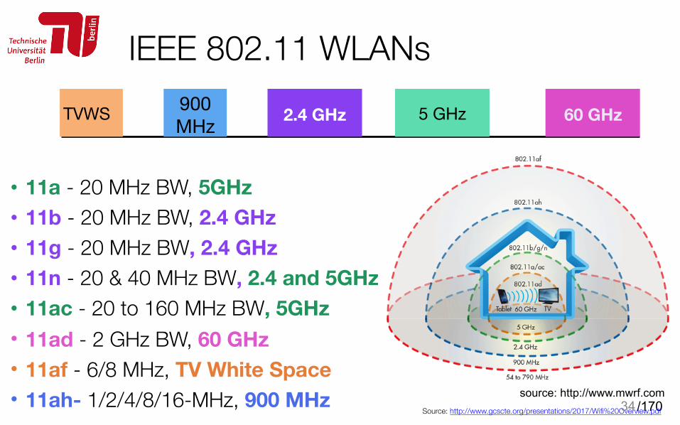
IEEE 802.11 WLANs
Source: http://www.gcscte.org/presentations/2017/Wifi%20Overview.pdf34
• 11a - 20 MHz BW, 5GHz • 11b - 20 MHz BW, 2.4 GHz • 11g - 20 MHz BW, 2.4 GHz • 11n - 20 & 40 MHz BW, 2.4 and 5GHz • 11ac - 20 to 160 MHz BW, 5GHz • 11ad - 2 GHz BW, 60 GHz • 11af - 6/8 MHz, TV White Space • 11ah- 1/2/4/8/16-MHz, 900 MHz
2.4 GHz 5 GHzTVWS 60 GHz900 MHz
source: http://www.mwrf.com

/170
Spectrum commons: Unlicensed bands
35
• 2.4 GHz ISM bands: already crowded - WiFi, Bluetooth, microwave ovens, Zigbee, etc. - WiFi: 802.11b/g/n at 2.4 GHz - Channels 1, 6, 11 are non-overlapping and should be used
• 5 GHz UNII bands: getting crowded - WiFi, Radar, unlicensed LTE - WiFi: 802.11a/n/ac at 5GHz and future standards 11ax - Non-overlapping 20+ channels of 20 MHz
/170
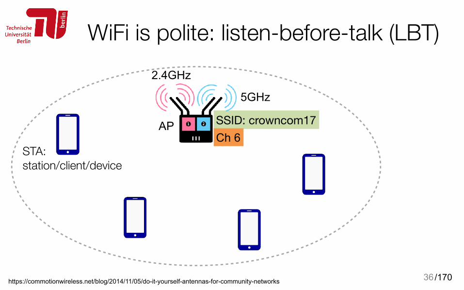
WiFi is polite: listen-before-talk (LBT)
36https://commotionwireless.net/blog/2014/11/05/do-it-yourself-antennas-for-community-networks
2.4GHz
5GHz
AP
STA: station/client/device
SSID: crowncom17Ch 6
/170
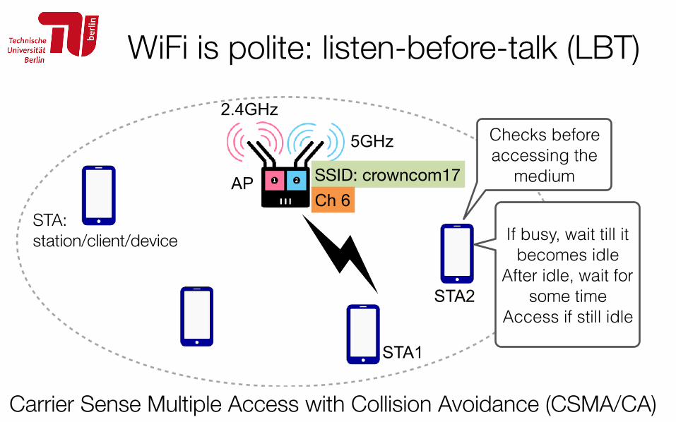
WiFi is polite: listen-before-talk (LBT)
37
Checks before accessing the
medium
If busy, wait till it becomes idle
After idle, wait for some time
Access if still idle
2.4GHz
5GHz
AP
STA: station/client/device
Carrier Sense Multiple Access with Collision Avoidance (CSMA/CA)
SSID: crowncom17Ch 6
STA1
STA2
/170
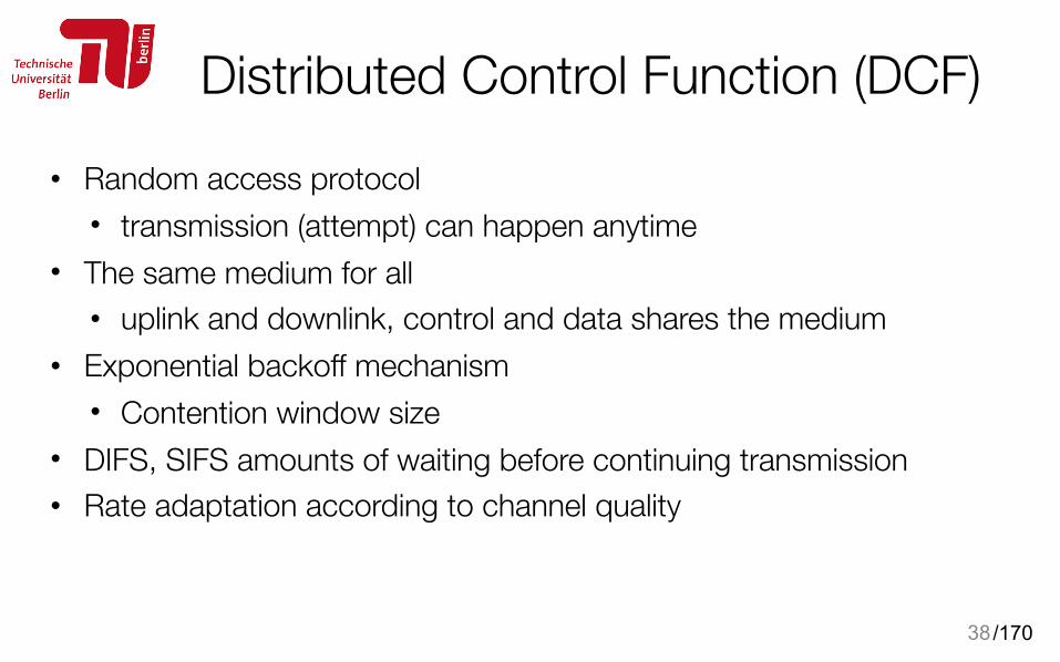
Distributed Control Function (DCF)• Random access protocol
• transmission (attempt) can happen anytime • The same medium for all
• uplink and downlink, control and data shares the medium • Exponential backoff mechanism
• Contention window size • DIFS, SIFS amounts of waiting before continuing transmission • Rate adaptation according to channel quality
38
/170
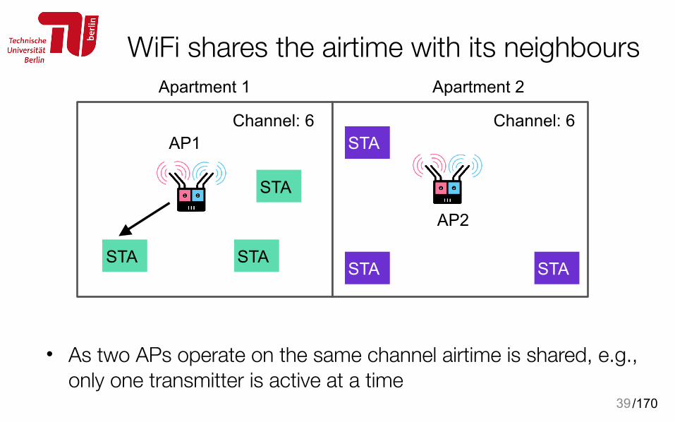
WiFi shares the airtime with its neighbours
• As two APs operate on the same channel airtime is shared, e.g., only one transmitter is active at a time
39
STA
STA
STASTA
STA
STA
AP1
AP2
Channel: 6 Channel: 6
Apartment 1 Apartment 2

/170
WiFi shares the airtime with its neighbours
40
STA
STA
STASTA
STA
STA
AP1
AP2
Channel: 6 Channel: 6
Apartment 1 Apartment 2
airtime (AP2)= 0.5airtime(AP1)= 0.5
/170
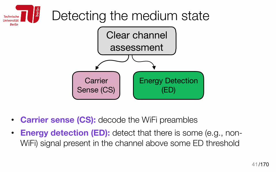
Detecting the medium state
• Carrier sense (CS): decode the WiFi preambles • Energy detection (ED): detect that there is some (e.g., non-
WiFi) signal present in the channel above some ED threshold
41
Clear channel assessment
Carrier Sense (CS)
Energy Detection(ED)

/170
• Carrier sense (CS): decode the WiFi preambles • Energy detection (ED): detect that there is some (e.g., non-
WiFi) signal present in the channel above some ED threshold
42
Clear channel assessment
Carrier Sense (CS)
Energy Detection(ED) -62 dBm-82 dBm
Detecting the medium state
/170
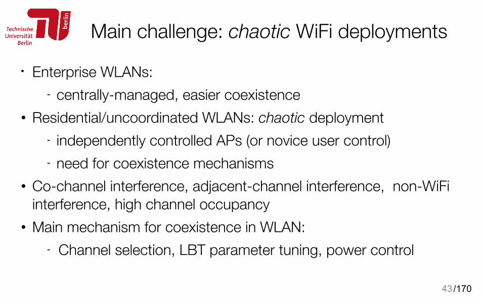
Main challenge: chaotic WiFi deployments
• Enterprise WLANs: - centrally-managed, easier coexistence
• Residential/uncoordinated WLANs: chaotic deployment - independently controlled APs (or novice user control) - need for coexistence mechanisms
• Co-channel interference, adjacent-channel interference, non-WiFi interference, high channel occupancy
• Main mechanism for coexistence in WLAN: - Channel selection, LBT parameter tuning, power control
43
/170
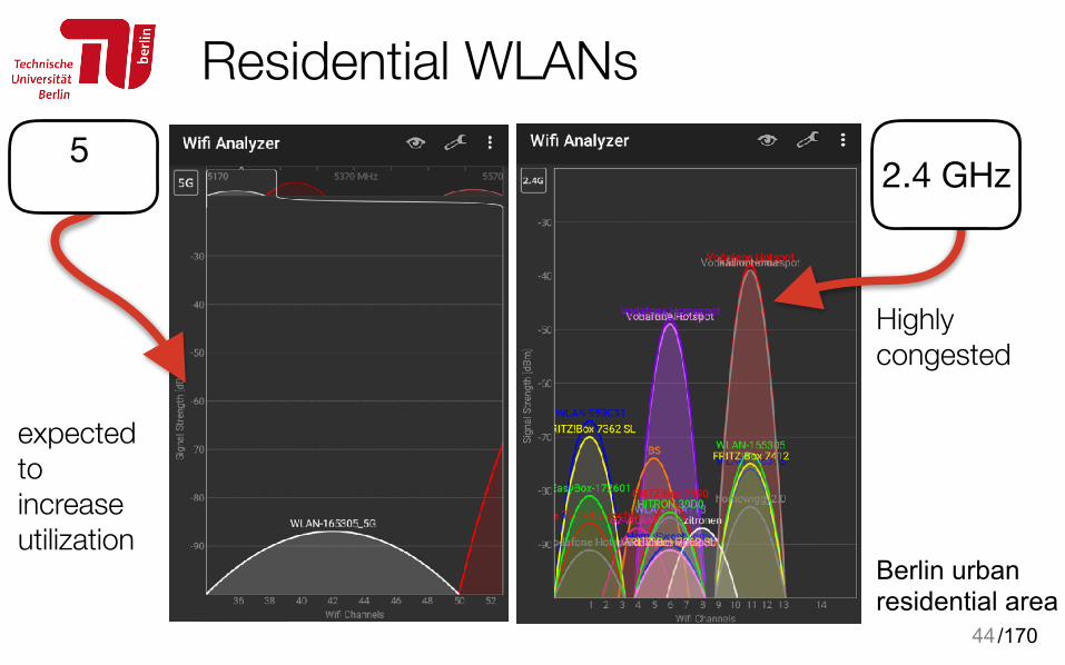
Residential WLANs
44
Berlin urban residential area
2.4 GHz
Highly congested
5
expected to increase utilization
/170
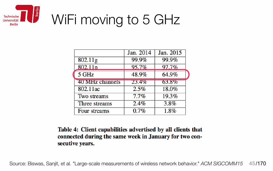
WiFi moving to 5 GHz
45Source: Biswas, Sanjit, et al. "Large-scale measurements of wireless network behavior." ACM SIGCOMM15

/170
A brief overview of unlicensed
46
/170
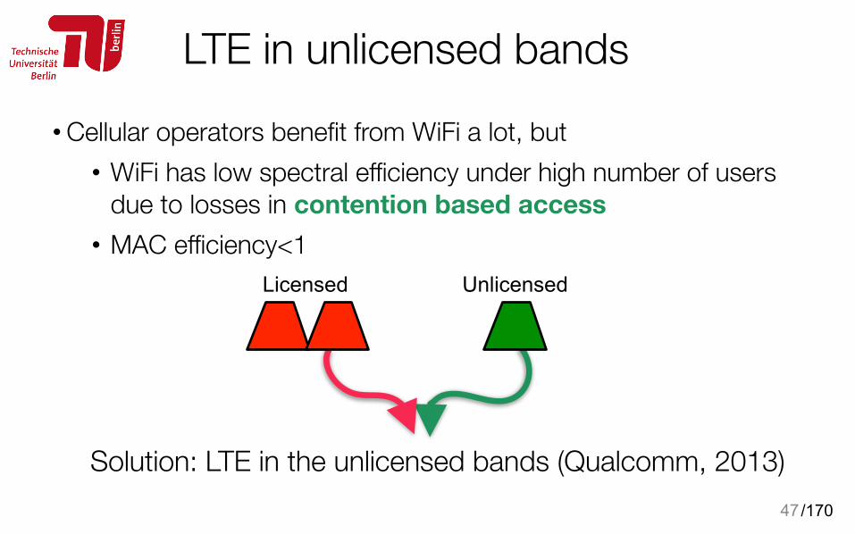
LTE in unlicensed bands• Cellular operators benefit from WiFi a lot, but
• WiFi has low spectral efficiency under high number of users due to losses in contention based access
• MAC efficiency<1
47
UnlicensedLicensed
Solution: LTE in the unlicensed bands (Qualcomm, 2013)
/170
Why LTE in unlicensed bands?•Unified control at the same core:
- authentication, management, and security procedures •higher spectral efficiency in the unlicensed bands
- Centrally-scheduled access •Better error control at LTE
- HARQ vs. ARQ • other interesting convergence solutions not discussed here:
MuLTEfire, LWA
48
/170
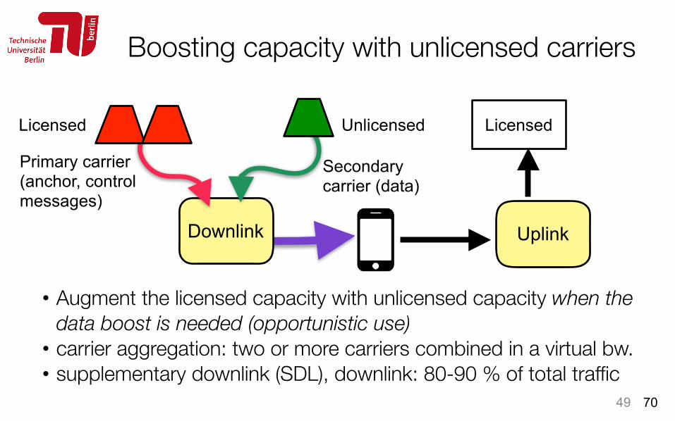
Downlink
Boosting capacity with unlicensed carriers
• Augment the licensed capacity with unlicensed capacity when the data boost is needed (opportunistic use)
• carrier aggregation: two or more carriers combined in a virtual bw. • supplementary downlink (SDL), downlink: 80-90 % of total traffic
49
Licensed
Primary carrier (anchor, control messages)
Secondary carrier (data)
Licensed Unlicensed
Uplink
/170
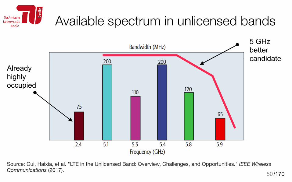
Available spectrum in unlicensed bands
50
Source: Cui, Haixia, et al. "LTE in the Unlicensed Band: Overview, Challenges, and Opportunities." IEEE Wireless Communications (2017).
Already highly occupied
5 GHz better candidate
/170
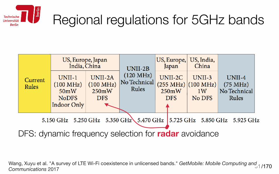
Regional regulations for 5GHz bands
DFS: dynamic frequency selection for radar avoidance
51Wang, Xuyu et al. "A survey of LTE Wi-Fi coexistence in unlicensed bands." GetMobile: Mobile Computing and Communications 2017
/170
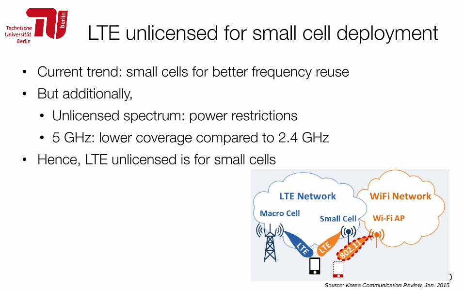
LTE unlicensed for small cell deployment• Current trend: small cells for better frequency reuse • But additionally,
• Unlicensed spectrum: power restrictions • 5 GHz: lower coverage compared to 2.4 GHz
• Hence, LTE unlicensed is for small cells
52
/170
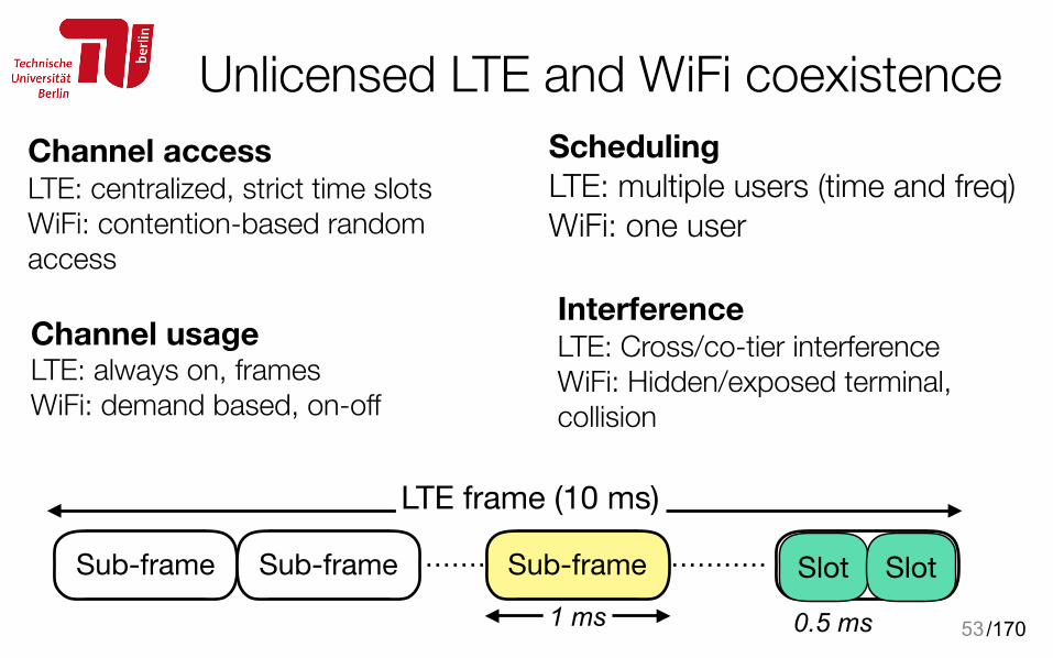
Unlicensed LTE and WiFi coexistence
530.5 ms
Sub-frame Sub-frame Sub-frame
LTE frame (10 ms)
1 ms
Sub-frame Slot Slot
Channel access LTE: centralized, strict time slots WiFi: contention-based random access
Channel usage LTE: always on, frames WiFi: demand based, on-off
Scheduling LTE: multiple users (time and freq) WiFi: one user
Interference LTE: Cross/co-tier interference WiFi: Hidden/exposed terminal, collision

/170
• Main problem: different PHY and MAC rules
Unlicensed LTE and WiFi coexistence
54
802.11a/n/acSomebody in the channel Exponential back off
• Expected result: WiFi suffers from LTE, if LTE does not adapt coexistence mechanisms!
LTE
/170
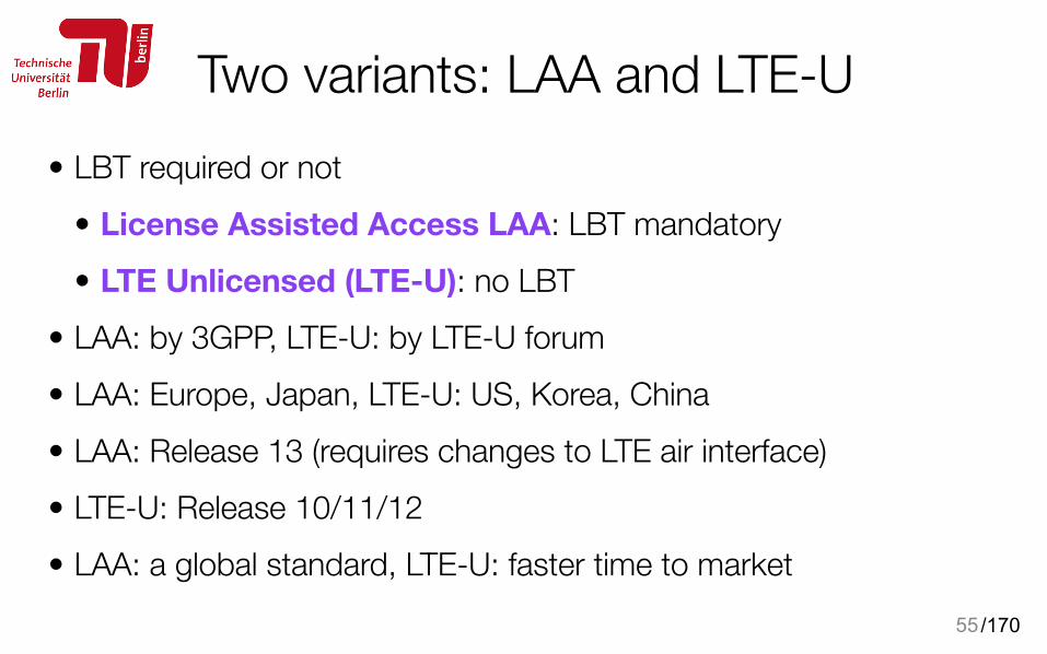
Two variants: LAA and LTE-U• LBT required or not
• License Assisted Access LAA: LBT mandatory • LTE Unlicensed (LTE-U): no LBT
• LAA: by 3GPP, LTE-U: by LTE-U forum • LAA: Europe, Japan, LTE-U: US, Korea, China • LAA: Release 13 (requires changes to LTE air interface) • LTE-U: Release 10/11/12 • LAA: a global standard, LTE-U: faster time to market
55
/170
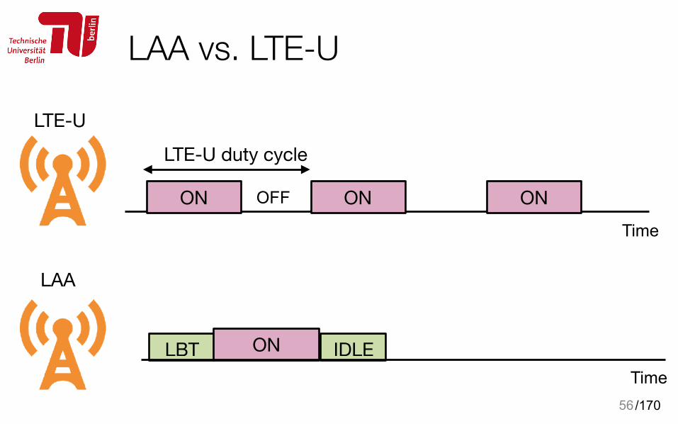
LAA vs. LTE-U
56
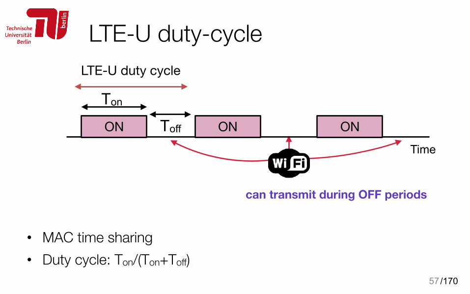
LTE-U duty cycle
OFF
LTE-U
LAA
LBT ON IDLE
ONONONTime
Time
/170
LTE-U duty-cycle
• MAC time sharing • Duty cycle: Ton/(Ton+Toff)
57
can transmit during OFF periods
Ton
Toff
LTE-U duty cycle
ONONONTime
/170
• MAC time sharing • Duty cycle: Ton/(Ton+Toff) • CSAT (carrier sense adaptive transmission): adaptive duty cycle • Adaptation according to WiFi medium utilisation and number of
WiFi nodes observed by user devices or small base stations
LTE-U duty-cycle
58
Ton
Toff ONONONTime
Medium sensing
/170
How to set the ON-OFF durations?• Medium sharing: if X is LTE’s duty-cycle, airtime for WiFi is (1-X) • But some caveats: • Length of ON-duration: WiFi has to wait till the end of ON
period which may affect latency-sensitive applications, e.g., high QoS frames.
59
/170
How to set the ON-OFF durations?• Medium sharing: if X is LTE’s duty-cycle, airtime for WiFi is (1-X) • But some caveats: • Length of ON-duration: WiFi has to wait till the end of ON
period which may affect latency-sensitive applications, e.g., high QoS frames. • subframe puncturing • max ON duration 20 ms
60
subframe puncturing period ~ 2 msec gaps
/170
How to set the ON-OFF durations?• Medium sharing: if X is LTE’s duty-cycle, airtime for WiFi is (1-X) • But some caveats: • Length of ON-duration: WiFi has to wait till the end of ON
period which may affect latency-sensitive applications, e.g., high QoS frames.
• Length of OFF-duration: typically 40/80 ms
61
ON
Packet collisionsRate adaptation (low rates)Exponential backoff
ON Off
backoff x
/170
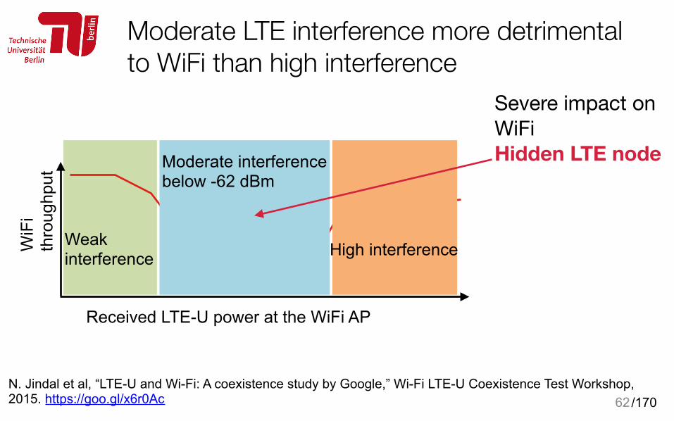
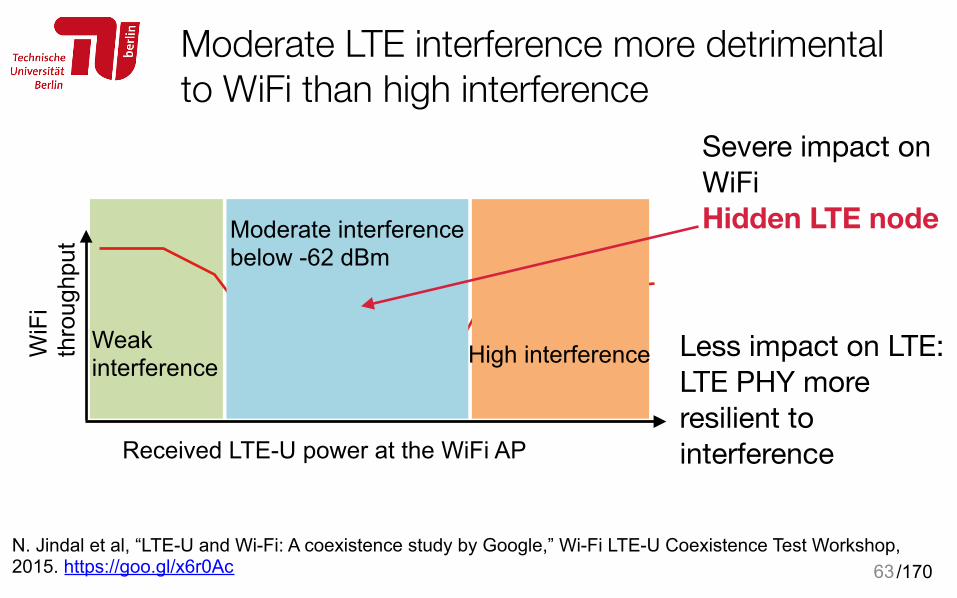
Moderate LTE interference more detrimental to WiFi than high interference
62N. Jindal et al, “LTE-U and Wi-Fi: A coexistence study by Google,” Wi-Fi LTE-U Coexistence Test Workshop, 2015. https://goo.gl/x6r0Ac
Received LTE-U power at the WiFi AP
Moderate interference below -62 dBm
WiF
i th
roug
hput
High interferenceWeak interference
Severe impact on WiFiHidden LTE node
/170
Moderate LTE interference more detrimental to WiFi than high interference
63N. Jindal et al, “LTE-U and Wi-Fi: A coexistence study by Google,” Wi-Fi LTE-U Coexistence Test Workshop, 2015. https://goo.gl/x6r0Ac
Received LTE-U power at the WiFi AP
Moderate interference below -62 dBm
High interferenceWeak interference
WiF
i th
roug
hput
Less impact on LTE: LTE PHY more resilient to interference
Severe impact on WiFiHidden LTE node
/170
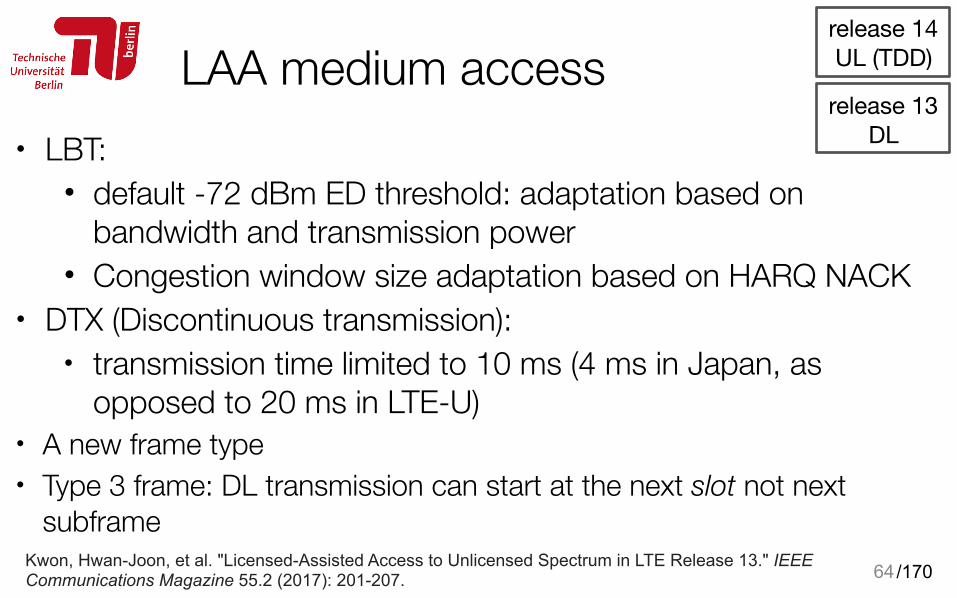
LAA medium access• LBT:
• default -72 dBm ED threshold: adaptation based on bandwidth and transmission power
• Congestion window size adaptation based on HARQ NACK • DTX (Discontinuous transmission):
• transmission time limited to 10 ms (4 ms in Japan, as opposed to 20 ms in LTE-U)
• A new frame type • Type 3 frame: DL transmission can start at the next slot not next
subframe 64Kwon, Hwan-Joon, et al. "Licensed-Assisted Access to Unlicensed Spectrum in LTE Release 13." IEEE
Communications Magazine 55.2 (2017): 201-207.
release 13DL
release 14UL (TDD)
/170
5 GHz not congested yet, but it is highly likely that it will soon
Coexistence mechanisms to be implemented
65
/170
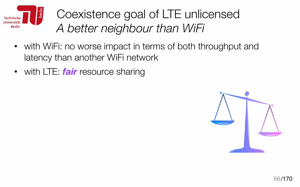
Coexistence goal of LTE unlicensed A better neighbour than WiFi
• with WiFi: no worse impact in terms of both throughput and latency than another WiFi network
• with LTE: fair resource sharing
66

/170
Peaceful Coexistence in Unlicensed Spectrum
67
/170
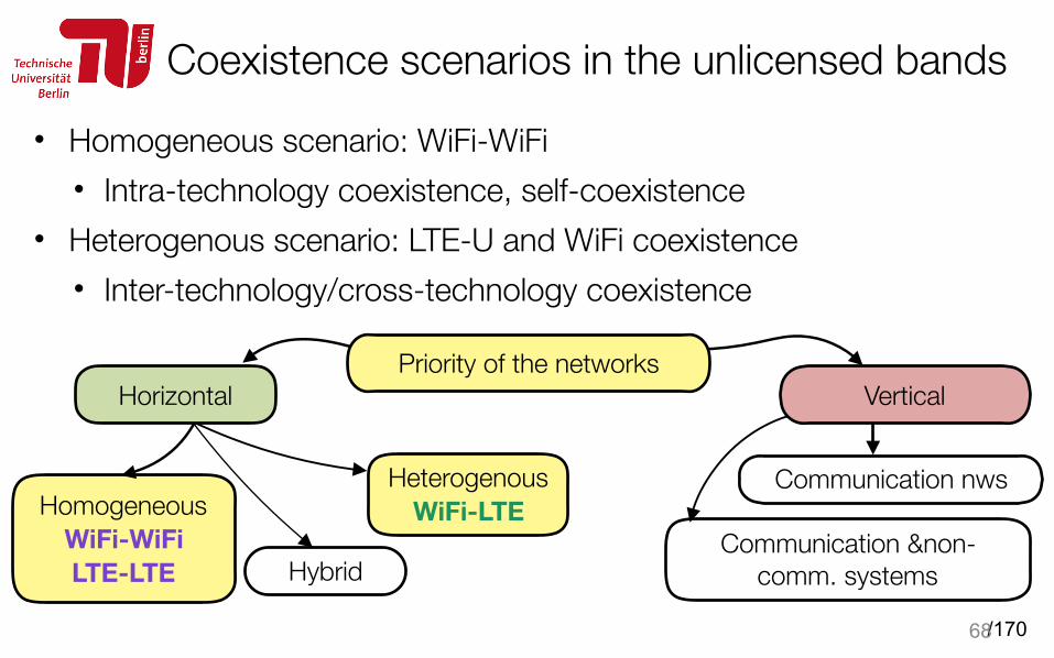
Coexistence scenarios in the unlicensed bands
• Homogeneous scenario: WiFi-WiFi • Intra-technology coexistence, self-coexistence
• Heterogenous scenario: LTE-U and WiFi coexistence • Inter-technology/cross-technology coexistence
68
Communication nws
Communication &non-comm. systems
Homogeneous WiFi-WiFi LTE-LTE
Heterogenous WiFi-LTE
Hybrid
Vertical Priority of the networks
Horizontal
/170
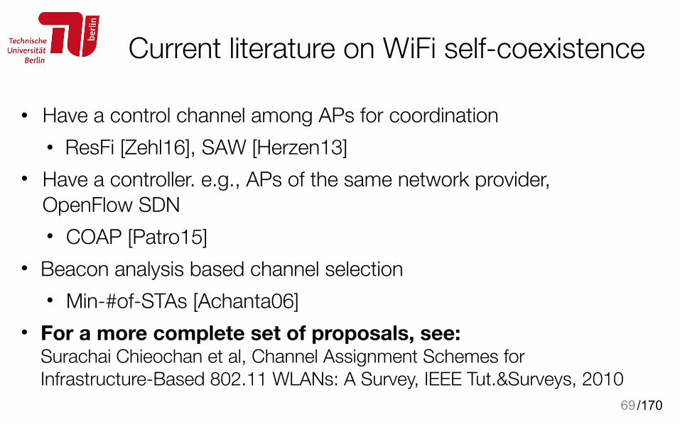
Current literature on WiFi self-coexistence
• Have a control channel among APs for coordination • ResFi [Zehl16], SAW [Herzen13]
• Have a controller. e.g., APs of the same network provider, OpenFlow SDN • COAP [Patro15]
• Beacon analysis based channel selection • Min-#of-STAs [Achanta06]
• For a more complete set of proposals, see:Surachai Chieochan et al, Channel Assignment Schemes for Infrastructure-Based 802.11 WLANs: A Survey, IEEE Tut.&Surveys, 2010
69
/170
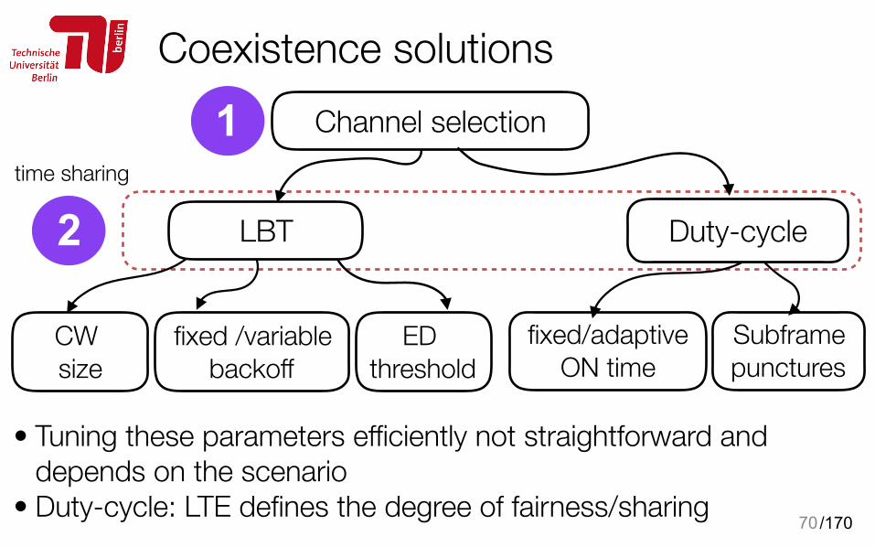
Coexistence solutions
70
time sharing
fixed /variable backoff
fixed/adaptive ON time
Channel selection
• Tuning these parameters efficiently not straightforward and depends on the scenario
• Duty-cycle: LTE defines the degree of fairness/sharing
CW size
LBT
ED threshold
Subframe punctures
Duty-cycle
1
2
/170
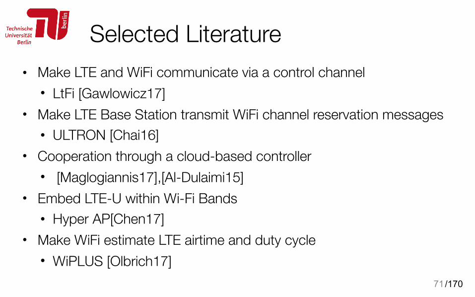
Selected Literature• Make LTE and WiFi communicate via a control channel
• LtFi [Gawlowicz17] • Make LTE Base Station transmit WiFi channel reservation messages
• ULTRON [Chai16] • Cooperation through a cloud-based controller
• [Maglogiannis17],[Al-Dulaimi15] • Embed LTE-U within Wi-Fi Bands
• Hyper AP[Chen17] • Make WiFi estimate LTE airtime and duty cycle
• WiPLUS [Olbrich17]71
/170
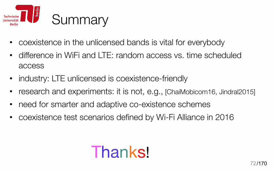
Summary• coexistence in the unlicensed bands is vital for everybody • difference in WiFi and LTE: random access vs. time scheduled
access
• industry: LTE unlicensed is coexistence-friendly • research and experiments: it is not, e.g., [ChaiMobicom16, Jindral2015]
• need for smarter and adaptive co-existence schemes • coexistence test scenarios defined by Wi-Fi Alliance in 2016
72Thanks!
/170
References• Florian Kaltenberger, Carrier Aggregation and License Assisted Access Evolution from LTE-Advanced to
5G, Summer school on Spectrum Sharing and Aggregation for 5G, 2016. • Chen et al. "Coexistence of LTE-LAA and Wi-Fi on 5 GHz with corresponding deployment scenarios: A
survey."IEEE Comm.SurveysTutorials, 2017. • 3GPP TS 36.101 / TS 36.521-1 for UE testing • 3GPP TS 36.104 / TS 36.141 for eNB testing • 3GPP, “Study on licensed-assisted access to unlicensed spectrum,” TR 36.889 TSG RAN, Rel. 13
v13.0.0, Jun. 2015 • Wang, Xuyu, Shiwen Mao, and Michelle X. Gong. "A survey of LTE Wi-Fi coexistence in unlicensed
bands." GetMobile: Mobile Computing and Communication, 2017 • Beltran, Fernando, Sayan Kumar Ray, and Jairo A. Gutiérrez. "Understanding the current operation and
future roles of wireless networks: Co-existence, competition and co-operation in the unlicensed spectrum bands." IEEE JSAC 2016.
• Voicu, Andra M., Ljiljana Simić, and Marina Petrova. "Inter-technology coexistence in a spectrum commons: A case study of Wi-Fi and LTE in the 5-GHz unlicensed band." IEEE JSAC 2016
73
/170
Part III A very brief overview of Machine Learning
74
20 • Supervised Learning • Unsupervised Learning • Reinforcement Learning
/170
An abstraction of a system in operation
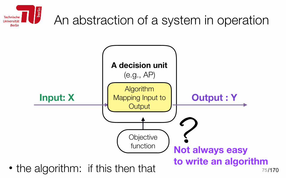
75
A decision unit (e.g., AP)
Objective function
Algorithm Mapping Input to
Output
• the algorithm: if this then that
?Not always easy to write an algorithm
Input: X Output : Y
/170
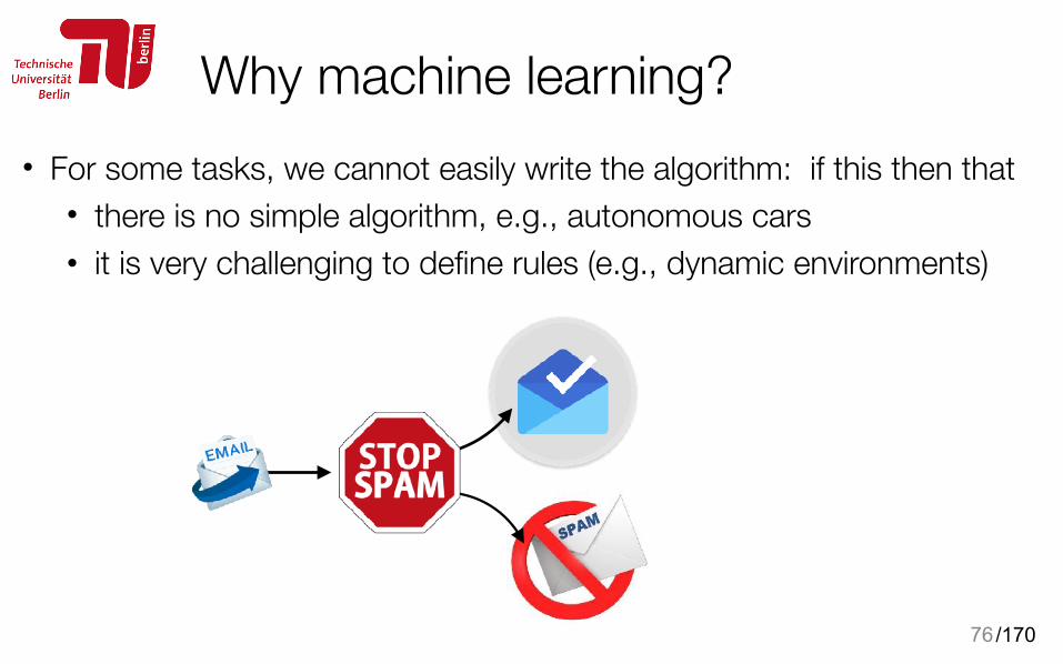
Why machine learning?• For some tasks, we cannot easily write the algorithm: if this then that
• there is no simple algorithm, e.g., autonomous cars • it is very challenging to define rules (e.g., dynamic environments)
76
/170
Learn from data or past experience
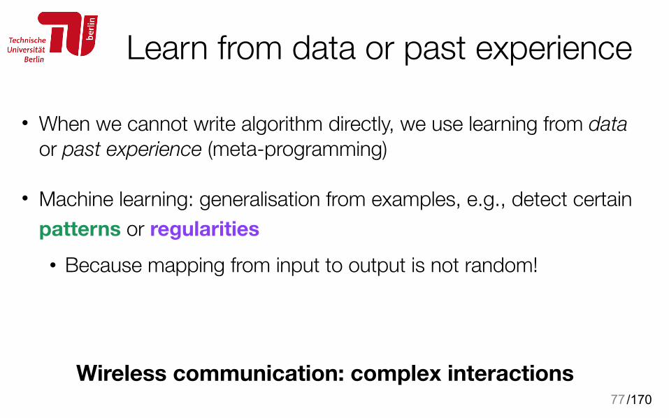
• When we cannot write algorithm directly, we use learning from data or past experience (meta-programming)
• Machine learning: generalisation from examples, e.g., detect certain patterns or regularities • Because mapping from input to output is not random!
77
Wireless communication: complex interactions
/170
How to learn the mapping?
78
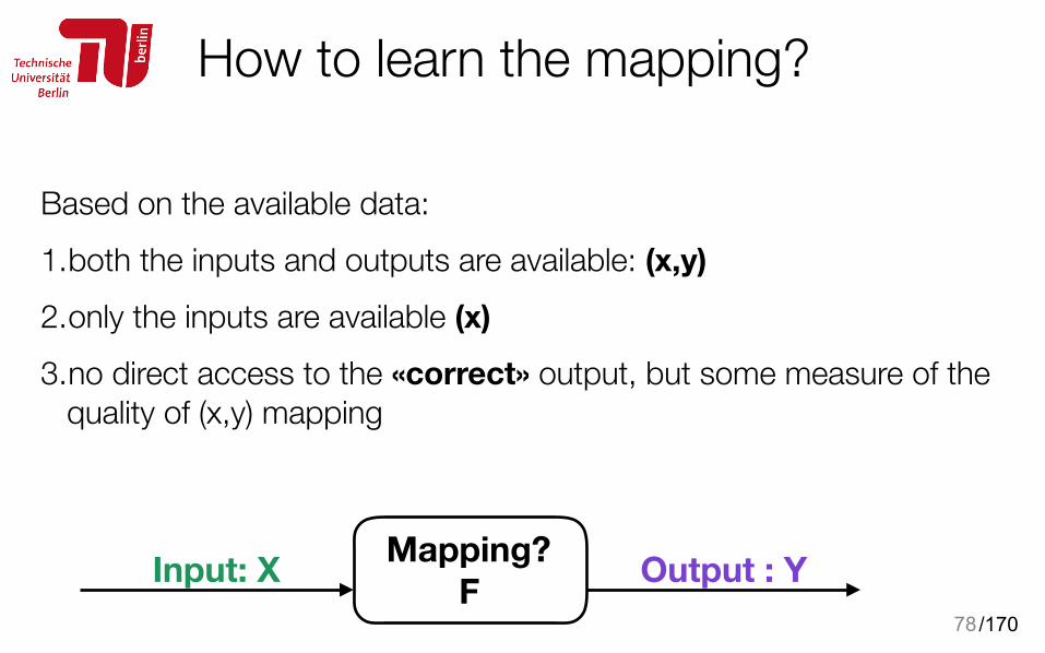
Based on the available data: 1.both the inputs and outputs are available: (x,y) 2.only the inputs are available (x) 3.no direct access to the «correct» output, but some measure of the
quality of (x,y) mapping
Input: X Output : YMapping? F
/170
{How to learn the mapping?
79
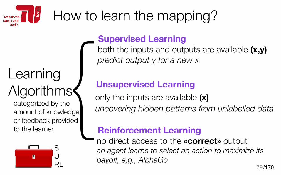
Unsupervised LearningLearning Algorithms
Supervised Learning
Reinforcement Learningno direct access to the «correct» output an agent learns to select an action to maximize its payoff, e,g., AlphaGo
only the inputs are available (x) uncovering hidden patterns from unlabelled data
both the inputs and outputs are available (x,y) predict output y for a new x
categorized by the amount of knowledge or feedback provided to the learner
SURL
/170
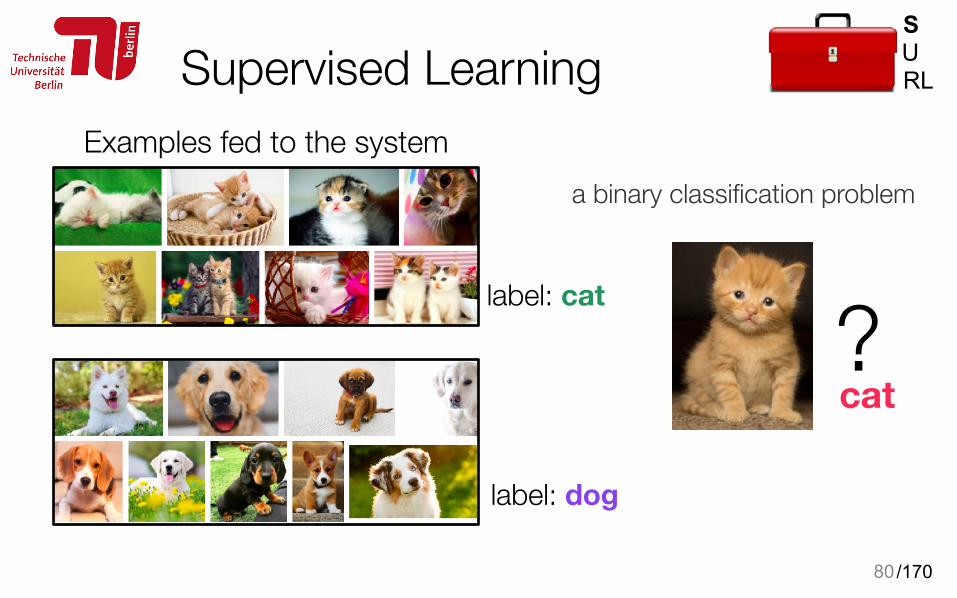
Supervised Learning
80
label: dog
Examples fed to the system
label: cat ?cat
a binary classification problem
SURL
/170
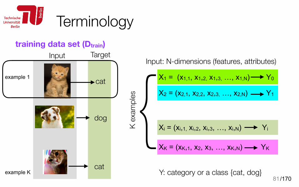
{Terminology
81
training data set (Dtrain)
cat
dog
cat
Input Target
example 1
example K
X1 = (x1,1, x1,2, x1,3, …, x1,N) Y0
X2 = (x2,1, x2,2, x2,3, …, x2,N) Y1
XK = (xK,1, x2, x3, …, xK,N) YK
Xi = (xi,1, xi,2, xi,3, …, xi,N) Yi
Input: N-dimensions (features, attributes)
K ex
ampl
es
Y: category or a class {cat, dog}
/170
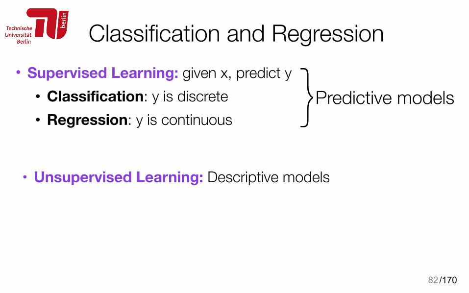
Classification and Regression• Supervised Learning: given x, predict y
• Classification: y is discrete • Regression: y is continuous
82
Predictive models{• Unsupervised Learning: Descriptive models
/170
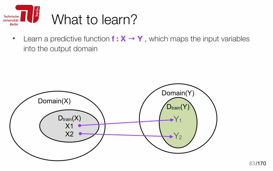
What to learn?• Learn a predictive function f : X → Y , which maps the input variables
into the output domain
83
Dtrain(X) X1 X2
Domain(X)Domain(Y)
Y1
Y2
Dtrain(Y)
/170
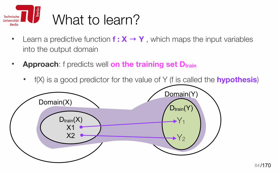
What to learn?• Learn a predictive function f : X → Y , which maps the input variables
into the output domain
• Approach: f predicts well on the training set Dtrain
• f(X) is a good predictor for the value of Y (f is called the hypothesis)
84
Dtrain(X) X1 X2
Domain(X)Domain(Y)
Y1
Y2
Dtrain(Y)
/170
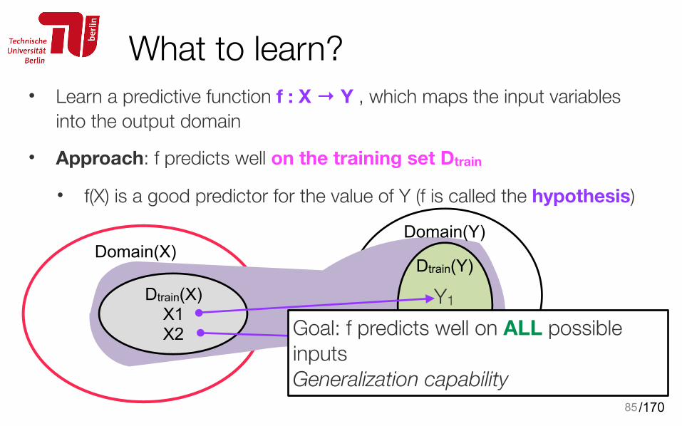
What to learn?• Learn a predictive function f : X → Y , which maps the input variables
into the output domain
• Approach: f predicts well on the training set Dtrain
• f(X) is a good predictor for the value of Y (f is called the hypothesis)
85
Dtrain(X) X1 X2
Domain(X)Domain(Y)
Y1
Y2
Dtrain(Y)
Goal: f predicts well on ALL possible inputs Generalization capability
/170
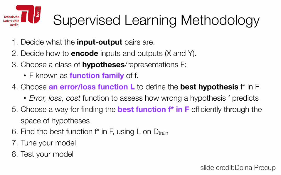
Supervised Learning Methodology1. Decide what the input-output pairs are. 2. Decide how to encode inputs and outputs (X and Y). 3. Choose a class of hypotheses/representations F:
• F known as function family of f. 4. Choose an error/loss function L to define the best hypothesis f* in F
• Error, loss, cost function to assess how wrong a hypothesis f predicts 5. Choose a way for finding the best function f* in F efficiently through the
space of hypotheses 6. Find the best function f* in F, using L on Dtrain
7. Tune your model 8. Test your model
86slide credit:Doina Precup
/170
Tune the model
Dataset split into three disjoint sets
87
Train the model
Learning algorithm Training data Dtrain
Feature vectors
Validation data Dvalid
Dataset (split into disjoint sets for train+validation and test 80-20, 70-30)
Assess the model
Test data Dtest
Loss function
RMSE, true positives, false positives
k-fold cross validation (k = 5 or 10)
/170
Bias-variance problem: overfitting, underfitting
•Underfit: model is too simple (high bias) • even the prediction error on Dtrain is high • Increase the complexity of the hypothesis
•Overfit: a model failing to generalize well (high variance) • learning even the noise or the random errors! Not desirable • add more training data • decrease complexity 88
Training data
/170
Checking for bias-variance error: validation data
89
ErrorValidation
Training
Tune the best parameter using validation data
Complexity of the hypothesis (degree of the polynomial)0 1 2 3 4 5
Remember that Dtrain and Dvalid and Dtest disjoint sets
/170
Checking for bias-variance error: validation data
90
ErrorValidation
Training
• Similarly, learning curves to see the number of training examples needed (better to have smarter data than smarter models)
# of training examples

/170
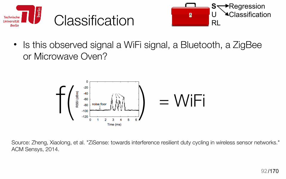
Classification• Is this observed signal a WiFi signal, a Bluetooth, a ZigBee
or Microwave Oven?
91
Source: Zheng, Xiaolong, et al. "ZiSense: towards interference resilient duty cycling in wireless sensor networks." ACM Sensys, 2014.
SURL
Regression Classification
/170
Classification• Is this observed signal a WiFi signal, a Bluetooth, a ZigBee
or Microwave Oven?
92
Source: Zheng, Xiaolong, et al. "ZiSense: towards interference resilient duty cycling in wireless sensor networks." ACM Sensys, 2014.
= WiFif( )
SURL
Regression Classification
/170
Classification algorithms
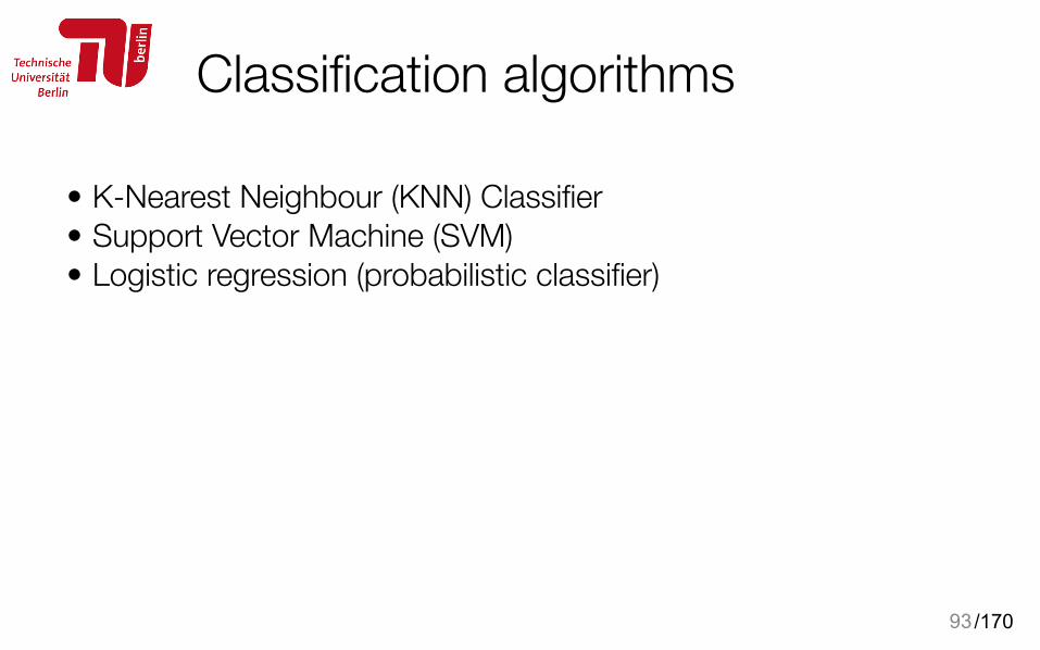
• K-Nearest Neighbour (KNN) Classifier • Support Vector Machine (SVM) • Logistic regression (probabilistic classifier)
93

/170
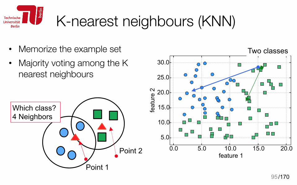
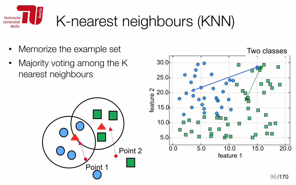
K-nearest neighbours (KNN)• Memorize the example set • Majority voting among the K
nearest neighbours
94
Two classes
/170
K-nearest neighbours (KNN)• Memorize the example set • Majority voting among the K
nearest neighbours
95
Two classes
Point 1
Point 2
Which class? 4 Neighbors
/170
K-nearest neighbours (KNN)• Memorize the example set • Majority voting among the K
nearest neighbours
96
Two classes
Point 1
Point 2
/170
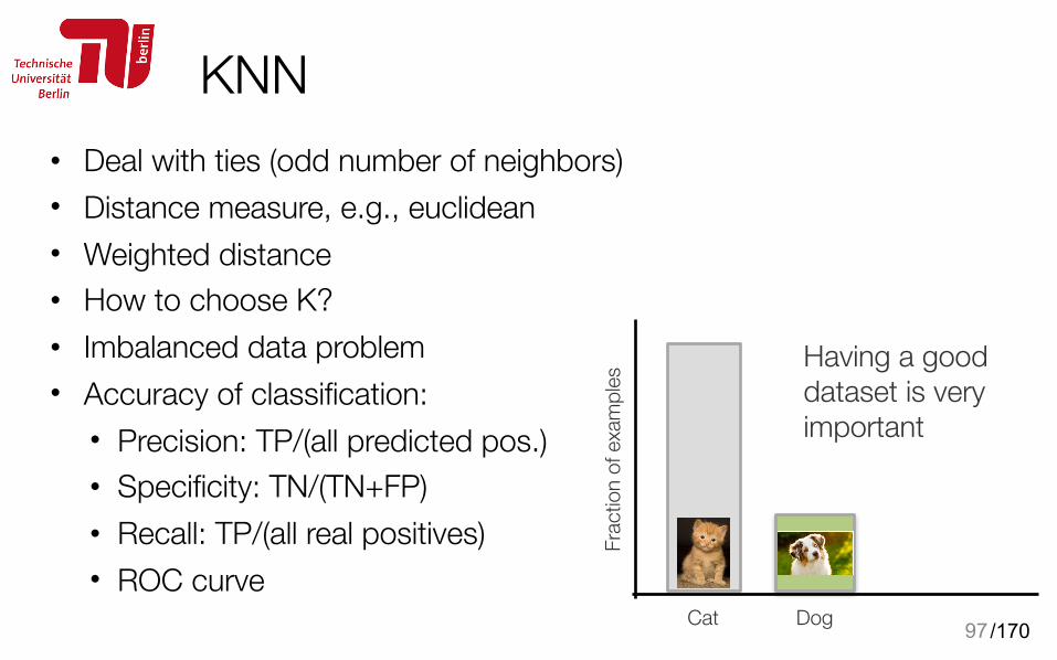
KNN• Deal with ties (odd number of neighbors) • Distance measure, e.g., euclidean • Weighted distance • How to choose K? • Imbalanced data problem • Accuracy of classification:
• Precision: TP/(all predicted pos.) • Specificity: TN/(TN+FP) • Recall: TP/(all real positives) • ROC curve
97Fr
actio
n of
exa
mpl
esCat Dog
Having a good dataset is very important
/170
Unsupervised Learning
• No labeled data • Can we group our data according to their feature? • The main goal is to classify or cluster the input, find outliers • Extracting useful information out of (big) data • Dimension reduction (or summarization): identify the
important components of the data while preserving much of the information
98
SURL
/170
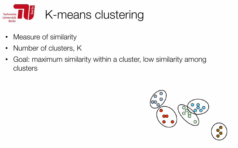
K-means clustering• Measure of similarity • Number of clusters, K • Goal: maximum similarity within a cluster, low similarity among
clusters
99
/170
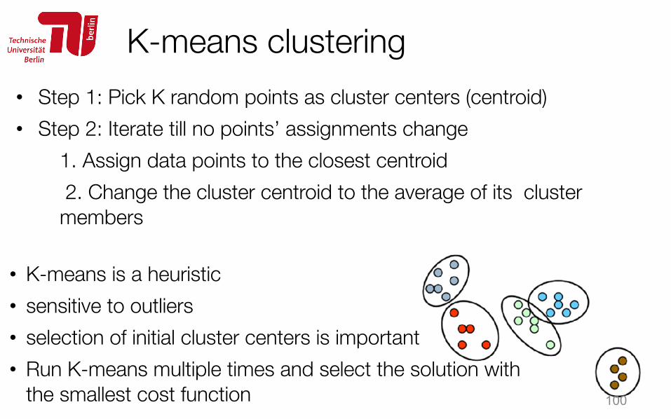
K-means clustering• Step 1: Pick K random points as cluster centers (centroid) • Step 2: Iterate till no pointsʼ assignments change
1. Assign data points to the closest centroid 2. Change the cluster centroid to the average of its cluster members
100
• K-means is a heuristic • sensitive to outliers • selection of initial cluster centers is important • Run K-means multiple times and select the solution with
the smallest cost function
/170
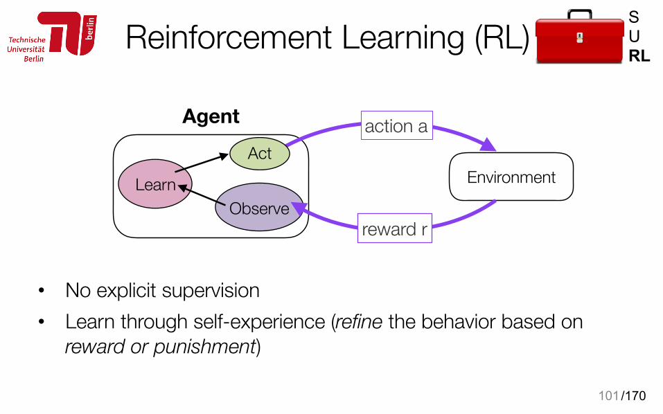
Reinforcement Learning (RL)
• No explicit supervision • Learn through self-experience (refine the behavior based on
reward or punishment)
101
Environment
ObserveLearn
Agent action aAct
reward r
SURL
/170
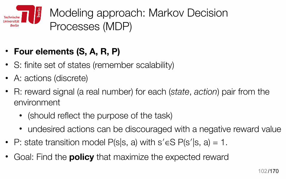
Modeling approach: Markov Decision Processes (MDP)
• Four elements (S, A, R, P) • S: finite set of states (remember scalability) • A: actions (discrete) • R: reward signal (a real number) for each (state, action) pair from the
environment • (should reflect the purpose of the task) • undesired actions can be discouraged with a negative reward value
• P: state transition model P(s|s, a) with s′∈S P(s′|s, a) = 1. • Goal: Find the policy that maximize the expected reward
102
/170
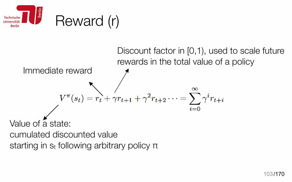
Reward (r)
103
Value of a state: cumulated discounted value starting in st following arbitrary policy π
Discount factor in [0,1), used to scale future rewards in the total value of a policy
Immediate reward
/170
Q-learning: the most popular RL method
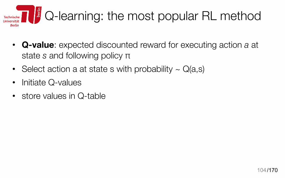
• Q-value: expected discounted reward for executing action a at state s and following policy π
• Select action a at state s with probability ~ Q(a,s) • Initiate Q-values • store values in Q-table
104
/170
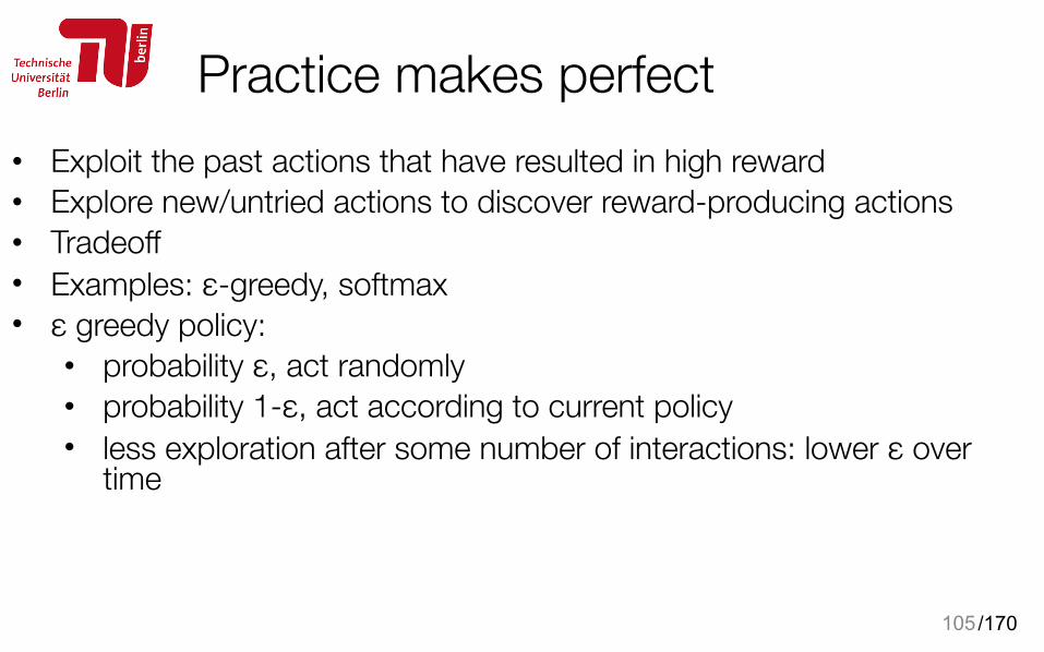
Practice makes perfect• Exploit the past actions that have resulted in high reward • Explore new/untried actions to discover reward-producing actions • Tradeoff • Examples: ε-greedy, softmax • ε greedy policy:
• probability ε, act randomly • probability 1-ε, act according to current policy • less exploration after some number of interactions: lower ε over
time
105
/170
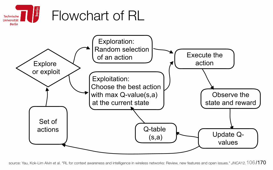
Flowchart of RL
source: Yau, Kok-Lim Alvin et al. "RL for context awareness and intelligence in wireless networks: Review, new features and open issues." JNCA12.106
Exploration: Random selection of an action
Exploitation: Choose the best action with max Q-value(s,a) at the current state
Observe the state and reward
Execute the actionExplore
or exploit
Set of actions
Update Q-values
Q-table (s,a)
/170
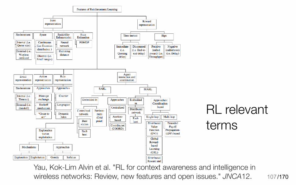
RL relevant terms
107Yau, Kok-Lim Alvin et al. "RL for context awareness and intelligence in wireless networks: Review, new features and open issues." JNCA12.
/170
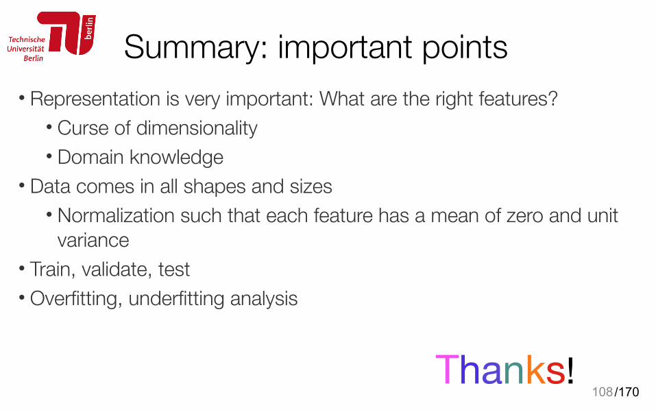
Summary: important points• Representation is very important: What are the right features?
• Curse of dimensionality • Domain knowledge
• Data comes in all shapes and sizes • Normalization such that each feature has a mean of zero and unit
variance • Train, validate, test • Overfitting, underfitting analysis
108Thanks!
/170
Please see below for more details• Pascal Vincent, Introduction to Machine Learning, Deep Learning Summer School, 2015. http://
videolectures.net/deeplearning2015_vincent_machine_learning/
• Doina Precup, Introduction to Machine Learning, Deep Learning Summer School, 2016. http://videolectures.net/deeplearning2016_precup_machine_learning/?q=Doina%20Precup
• Kulin, Merima, et al. "Data-driven design of intelligent wireless networks: An overview and tutorial." Sensors 16.
• Yau, Kok-Lim Alvin et al. "Reinforcement learning for context awareness and intelligence in wireless networks: Review, new features and open issues." JNCA12.
• Jiang, Chunxiao, et al. "Machine learning paradigms for next-generation wireless networks." IEEE Wireless Communications 24.2 (2017): 98-105.
• Bkassiny, Mario, Yang Li, and Sudharman K. Jayaweera. "A survey on machine-learning techniques in cognitive radios." IEEE Communications Surveys & Tutorials 15.3 (2013): 1136-1159.
• Ding, Guoru, et al. "Kernel-based learning for statistical signal processing in cognitive radio networks: Theoretical foundations, example applications, and future directions." IEEE Signal Processing Magazine 30.4 (2013): 126-136.
109
/170
Part IV Machine Learning for Coexistence in Wireless
Networks
110
/170
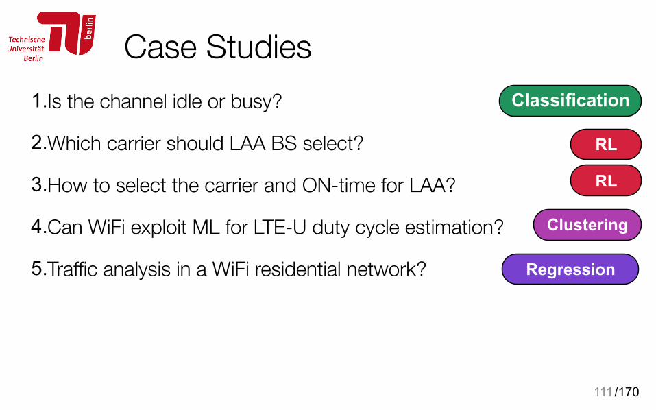
Case Studies1.Is the channel idle or busy?
2.Which carrier should LAA BS select?
3.How to select the carrier and ON-time for LAA?
4.Can WiFi exploit ML for LTE-U duty cycle estimation?
5.Traffic analysis in a WiFi residential network?
111
Classification
Regression
RL
RL
Clustering

/170
Attention!Please see the original papers for more details
ACK: figures are adapted or copied from the relevant papers
112
/170
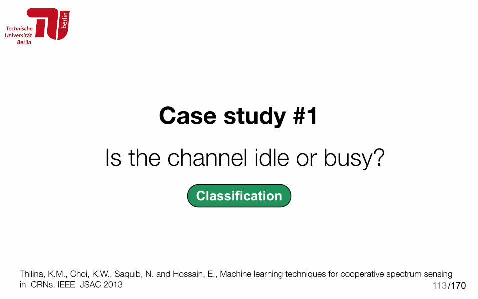
Case study #1 Is the channel idle or busy?
113
Classification
Thilina, K.M., Choi, K.W., Saquib, N. and Hossain, E., Machine learning techniques for cooperative spectrum sensing in CRNs. IEEE JSAC 2013
/170
Is the channel idle or busy?
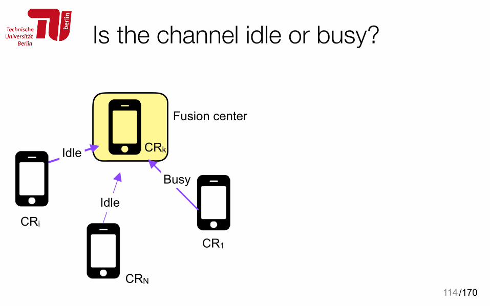
114
CR1
CRN
CRi
CRk
Fusion center
Idle
Busy
Idle
/170
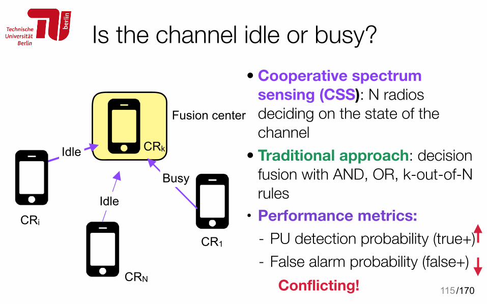
Is the channel idle or busy?• Cooperative spectrum
sensing (CSS): N radios deciding on the state of the channel
• Traditional approach: decision fusion with AND, OR, k-out-of-N rules
• Performance metrics: - PU detection probability (true+) - False alarm probability (false+)
115
CR1
CRN
CRi
CRk
Fusion center
Idle
Busy
Idle
Conflicting!
/170
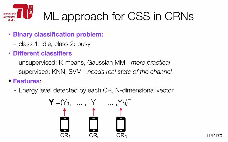
ML approach for CSS in CRNs
116
• Binary classification problem: - class 1: idle, class 2: busy
• Different classifiers - unsupervised: K-means, Gaussian MM - more practical - supervised: KNN, SVM - needs real state of the channel
• Features: - Energy level detected by each CR, N-dimensional vector
CR1 CRN
Y =(Y1, ... , Yj , ... ,YN)T
CRi
/170
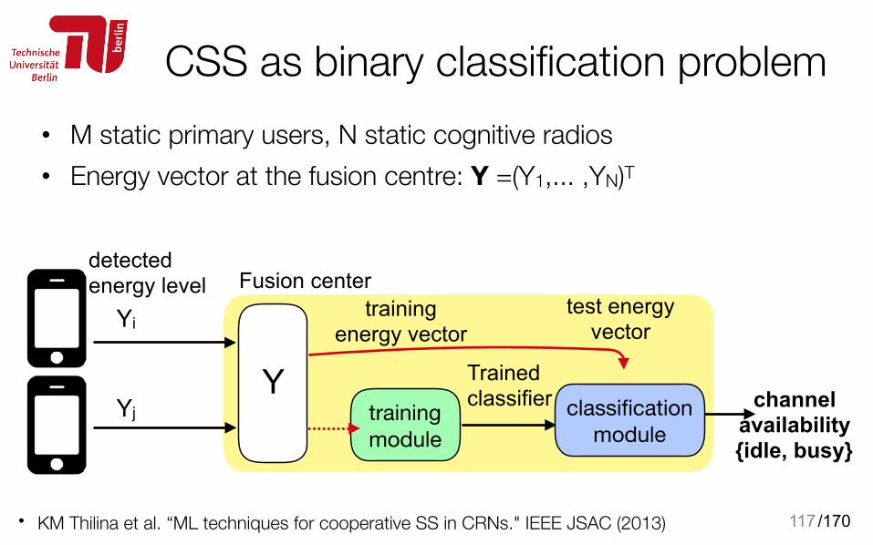
CSS as binary classification problem• M static primary users, N static cognitive radios • Energy vector at the fusion centre: Y =(Y1,... ,YN)T
117• KM Thilina et al. “ML techniques for cooperative SS in CRNs." IEEE JSAC (2013)
channel availability {idle, busy}
test energy vector
training energy vector
Trained classifier
Fusion center
Yi
Yj
detected energy level
training module
Yclassification
module
/170
Unsupervised learning for CSS
118
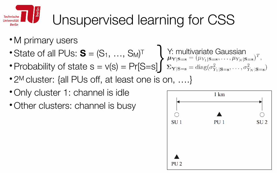
• M primary users • State of all PUs: S = (S1, …, SM)T
• Probability of state s = v(s) = Pr[S=s] • 2M cluster: {all PUs off, at least one is on, ….} • Only cluster 1: channel is idle • Other clusters: channel is busy
}Y: multivariate Gaussian
/170
Unsupervised learning for CSS• Decision boundary: idle vs. busy
119
Energy Level of SU1En
ergy
Lev
el o
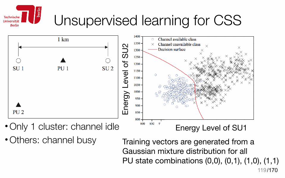
f SU
2• Only 1 cluster: channel idle • Others: channel busy Training vectors are generated from a
Gaussian mixture distribution for allPU state combinations (0,0), (0,1), (1,0), (1,1)
/170
Unsupervised learning for CSS• Decision boundary: idle vs. busy
120
Energy Level of SU1En
ergy
Lev
el o
f SU
2
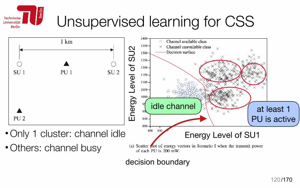
at least 1 PU is active
idle channel
• Only 1 cluster: channel idle • Others: channel busy
decision boundary
/170
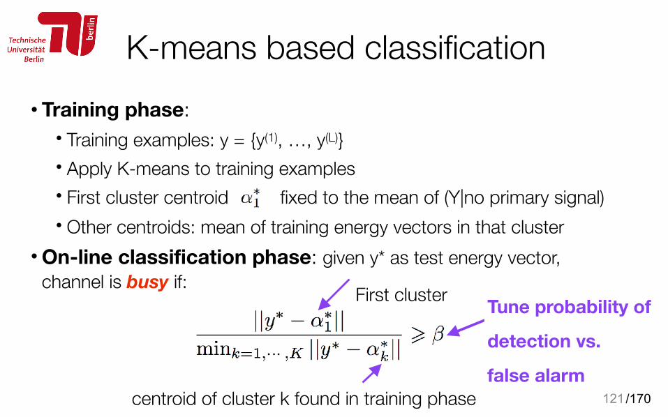
K-means based classification • Training phase:
• Training examples: y = {y(1), …, y(L)} • Apply K-means to training examples • First cluster centroid fixed to the mean of (Y|no primary signal) • Other centroids: mean of training energy vectors in that cluster
• On-line classification phase: given y* as test energy vector, channel is busy if:
121
Tune probability of
detection vs.
false alarmcentroid of cluster k found in training phase
First cluster
/170
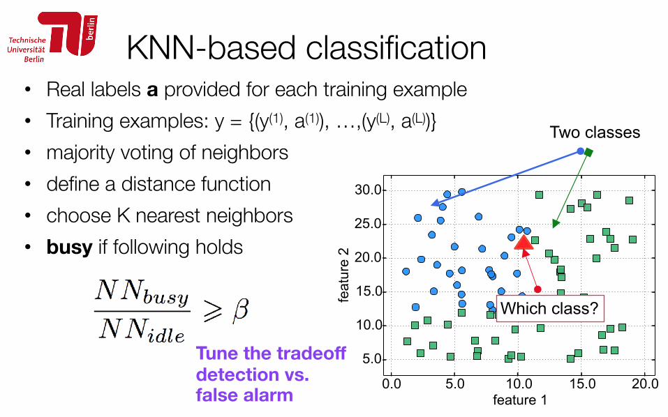
KNN-based classification• Real labels a provided for each training example • Training examples: y = {(y(1), a(1)), …,(y(L), a(L))} • majority voting of neighbors • define a distance function • choose K nearest neighbors • busy if following holds
122
Two classes
Which class?
Tune the tradeoff detection vs. false alarm
/170
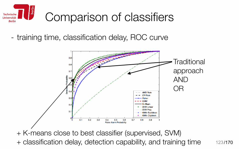
Comparison of classifiers- training time, classification delay, ROC curve
123
Traditional approach AND OR
+ K-means close to best classifier (supervised, SVM) + classification delay, detection capability, and training time

/170
Case study #2 Which carrier should LAA BS select?
124Sallent, O., Pérez-Romero, J., Ferrús, R. and Agustí, R., 2015, June. Learning-based coexistence for LTE operation in unlicensed bands 2015 IEEE International Conference on Communication Workshop
RL
/170
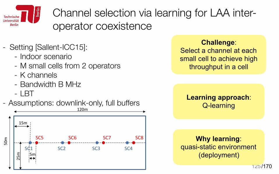
Channel selection via learning for LAA inter-operator coexistence
125
- Setting [Sallent-ICC15]: - Indoor scenario - M small cells from 2 operators - K channels - Bandwidth B MHz - LBT
- Assumptions: downlink-only, full buffers
Challenge: Select a channel at each small cell to achieve high
throughput in a cell
Learning approach: Q-learning
Why learning: quasi-static environment
(deployment)
situations like the hidden node problem where a small cell can detect a channel as not used but some of its served terminals can experience severe interference conditions from other small cells and/or Wi-Fis. Furthermore, including adaptability to the learning-based decision-making process will provide robustness to the solution and the capability to react to changes in the scenario (e.g., the deployment of a new small cell in the area).
With all the above, this paper proposes the use of a Q-learning solution as an efficient means to carry out a distributed Channel Selection in a practical while at the same time efficient way. Q-learning belongs to the category of Temporal Difference Reinforcement Learning (RL) techniques that consist in learning how to map situations to actions so as to maximize a scalar reward [16]. The learning is achieved through the interaction with the environment, so that the learner discovers which actions yield the most reward by trying them. In this way, the idea proposed by this paper is that each small cell progressively learns and selects the channels that provide the best performance based on the previous experience.
In particular, in the proposed approach each small cell i stores a value function Q(i,k) that measures the expected reward that can be achieved by using each channel k according to the past experience. Whenever a channel k has been used by the small cell i, the value function Q(i,k) is updated following a single state Q-learning approach with null discount rate given by [16]:
( ) ( ) ( ) ( ), 1 , · ,L LQ i k Q i k r i kα α← − + (2)
where αL∈(0,1) is the learning rate and r(i,k) is the reward that has been obtained as a result of the current use of the channel k. Assuming that the target of the channel selection is to find a channel that maximizes the total throughput, the reward function considered in this paper is given by:
( ) ( )max
,,
R i kr i k
R= (3)
where ( ),R i k is the average throughput that has been obtained
by the i-th small cell in channel k as a result of the last selection of this channel. In turn, ( )max max· · 1 idleR B S θ= − is a
normalization factor.
At initialization, i.e. when channel k has never been used in the past by small cell i, Q(i,k) is set to an arbitrary value Qini.
Based on the Q(i,k) value functions, the proposed Channel Selection decision-making for the small cell i follows the softmax policy [16] in which channel k is chosen with probability:
( )( )( )
( )( )
,
, '
' 1
Pr ,
Q i ki
Q i kKi
k
ei k
e
τ
τ
=
=
∑
(4)
where τ(i) is a positive parameter called temperature. High temperature values cause the different channels to be all nearly
equiprobable. Low temperature causes a greater difference in selection probability for channels that differ in their Q(i,k) value estimates, and the higher the value of Q(i,k) the higher the probability of selecting channel k. Softmax decision making is a popular means of balancing the exploitation and exploration dilemma in RL-based schemes. It exploits what the system already knows in order to obtain reward (i.e. selecting with high probability those channels that have provided good results in the past), but it also explores in order to make better actions in the future (i.e. the selection must try first a variety of channels and progressively favor those that appear to be the best ones) [16]. A cooling function will be considered in this paper to reduce the value of the temperature τ(i) as the number of channel selections made by the small cell i increases, so that the amount of exploration will be progressively decreased as the small cell has learnt the best solutions. Specifically, the following logarithmic cooling function is assumed [17]:
( ) ( )( )0
2log 1i
n iττ =+
(5)
where τ0 is the initial temperature and n(i) is the number of channel selections that have been already done by the i-th small cell.
IV. PERFORMANCE ANALYSIS
This section presents some evaluation results to illustrate the behavior and the performance of the proposed approach. A. Simulation scenario
The considered scenario is based on the indoor scenario for LTE-U coexistence evaluations defined in the context of the corresponding 3GPP Study Item [3]. It consists of a single floor building where two operators deploy 4 small cells (SCs) each. SCs are equally spaced and centered along the shorter dimension of the building, as depicted in Fig. 2. Small cells SC1 to SC4 are owned by operator 1 (OP1), while SC5 to SC8 are owned by operator 2 (OP2). SCs are deployed at height 6m while the antenna height of the mobile terminals is 1.5m. A total of 10 terminals (users) per operator are randomly distributed inside the building. Each user is associated to the SC of its own operator that provides the highest received power. The SC-to-terminal and SC-to-SC path loss and shadowing are computed using the ITU InH model in [18]. The carrier frequency is 5 GHz and the channel bandwidth B=20 MHz. The transmit power in one LTE-U carrier is 15 dBm. Omnidirectional antenna patterns are assumed with a total antenna gain plus connector loss of 5 dB. The terminal noise figure is 9 dB. The spectrum efficiency function S(SINR) is obtained from Section A.1 in [15] with Smax=4.4 b/s/Hz.
Fig. 2. Layout of the floor building
SC1 SC2 SC3 SC4
SC5 SC6 SC7 SC8
5m
50m
25m
120m
15m
IEEE ICC 2015 - Workshop on LTE in Unlicensed Bands: Potentials and Challenges
2310
/170
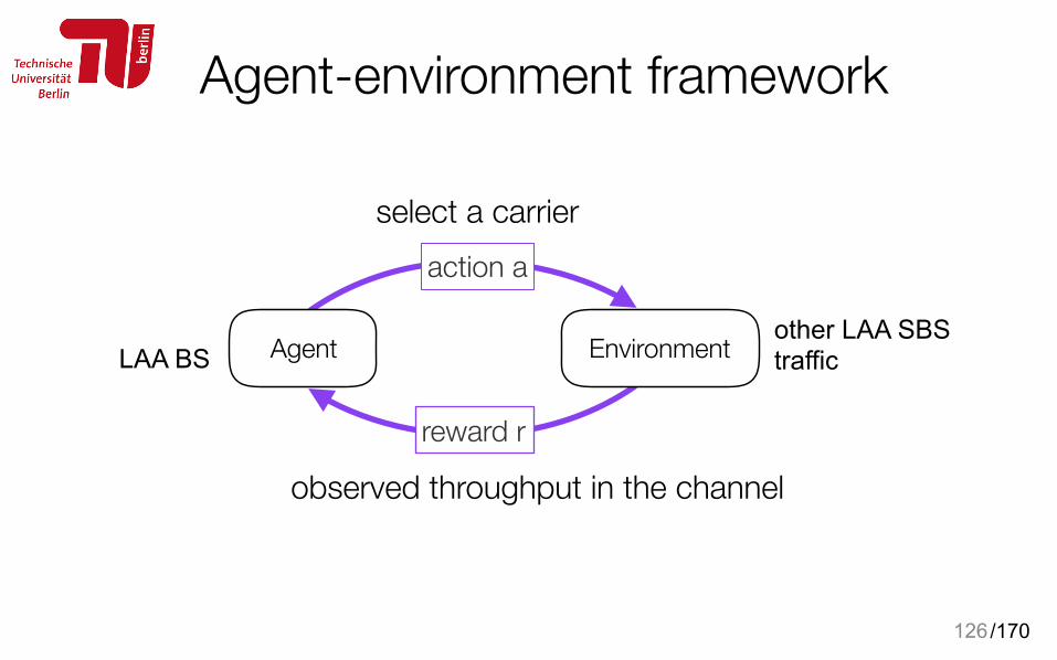
Agent-environment framework
126
action a
reward r
AgentLAA BS Environment other LAA SBS traffic
select a carrier
observed throughput in the channel
/170
Channel selection via learning for LAA inter-operator coexistence
• Reward: observed throughput in the channel • Q-value (k, i) for small cell i if it selects channel k • Initiate Q-values to some random value
127
reward of the transmission at ch k:throughput normalised by maximum exp. throughput
Learning rate
• Select a channel k with probability Pk ~ F(Q(i,k))• F: exploitation vs. exploration (softmax)• Decrease exploration by time (logarithmic cooling function)
/170
time steps. It can be observed how the initial solution learnt until t=30000 reflects that SC1 and SC4 learn to use channel k=3 (i.e. the only channel not used by OP2 at the beginning). This is certainly a good choice, since SC1 and SC4 are located far away from one another inside the building (see the layout in Fig. 2) so they are not mutually detected during the CCA phase (i.e., the received power level is below the TL threshold). Therefore, they can use the same channel without sharing it in the time domain. Similarly, SC2 learns to use the same channel k=4 as SC8, which is also located at a sufficiently large distance from SC2. As for SC3, it is located in the middle of the building and it is able to detect all the other SCs during the CCA phase, so it necessarily has to share a channel in the time domain following LBT. As seen in Fig. 6, it learns not to use channels k=3 and 4, which are already in use by two other SCs. Instead, it can use indifferently either channel k=1 or 2 as both of them are used only by another SC. As both channels provide the same performance, they are selected with equal probability.
After t=30000, SC7 is switched on and starts using channel k=3, which is the channel that was being used by SC1 and SC4 so far. Since SC1 is located at a sufficient distance from SC7 in order not to detect it during CCA, it keeps on operating in the same channel k=3, as seen in Fig. 6. Instead, SC4, located close to SC7, perceives throughput degradation in this channel due to the time sharing between SC4 and SC7, and progressively reduces its selection probability. At the end, SC4 learns to use the same channel k=1 as SC5 that is located at the other side of the building. With all these changes, also SC3 identifies that channel k=1 is no longer a good option (since it is used by both SC4 and SC5) and it learns to use channel k=2. The final solution learnt by the small cells of OP1 is the use of channels k=3,4,2,1, respectively by SC1 to SC4. A detailed analysis of the throughput achievable with all
the possible solutions (not reported for the sake of brevity) reveals that this is actually the solution that maximizes the total aggregated throughput among all the SCs of both operators. C. Performance analysis
In order to assess the benefits of the proposed solution from a quantitative perspective, Fig. 7 plots the ratio between the total throughput achieved by the proposed Q-learning in the scenario with respect to the throughput that would be achieved with an ideal optimum assignment. This optimum solution corresponds to the assignment of channels to small cells that maximizes the total throughput in the scenario. Results are provided for the cases K=4 and K=8 channels, and for the cases when Q-learning is applied only by OP 1 (OP 2 following a fixed assignment) or by the two operators. Each result corresponds to the average throughput obtained after 50 different experiments each one associated with a different user spatial distribution. Each experiment lasts for 1E6 time steps and the throughput for all SCs is aggregated and averaged along the whole simulation time. In each experiment the optimum channel assignment is found by exhaustive analysis of all the possible combinations.
As it can be observed in Fig. 7, the proposed approach achieves between 95.8 and 98.8% of the optimum throughput, revealing a promising behavior of the Q-learning mechanism. Reasonably, slightly better results are achieved with K=8 than with K=4, which is a more challenging scenario. Similarly, slightly better results are achieved when both operators apply Q-learning than when only one is doing so. In turn, Fig. 8 depicts the Cumulative Distribution Function (CDF) of the throughput (normalized to Rmax) obtained for all the considered experiments. The figure considers that both operators apply Q-learning with K=4 channels. It can be noticed how the
Fig. 5. Evolution of the channel selection probabilities with K=8 channels when both operators apply Q-learning.
0 1 2 3 4 5 6
x 104
0
0.2
0.4
0.6
0.8
1SC1
Time steps
0 1 2 3 4 5 6
x 104
0
0.2
0.4
0.6
0.8
1SC2
Time steps
0 1 2 3 4 5 6
x 104
0
0.2
0.4
0.6
0.8
1SC3
Time steps
0 1 2 3 4 5 6
x 104
0
0.2
0.4
0.6
0.8
1SC4
Time steps
Pr(k=1)Pr(k=2)Pr(k=3)Pr(k=4)Pr(k=5)Pr(k=6)Pr(k=7)Pr(k=8)
0 1 2 3 4 5 6
x 104
0
0.2
0.4
0.6
0.8
1SC5
Time steps
0 1 2 3 4 5 6
x 104
0
0.2
0.4
0.6
0.8
1SC6
Time steps
0 1 2 3 4 5 6
x 104
0
0.2
0.4
0.6
0.8
1SC7
Time steps
0 1 2 3 4 5 6
x 104
0
0.2
0.4
0.6
0.8
1SC8
Time steps
Pr(k=1)Pr(k=2)Pr(k=3)Pr(k=4)Pr(k=5)Pr(k=6)Pr(k=7)Pr(k=8)
Fig. 6. Evolution of the channel selection probabilities for the SCs of operator 1with K=4 channels when a new SC is activated at t=30000.
0 1 2 3 4 5 6
x 104
0
0.2
0.4
0.6
0.8
1SC1
Time steps
0 1 2 3 4 5 6
x 104
0
0.2
0.4
0.6
0.8
1SC2
Time steps
0 1 2 3 4 5 6
x 104
0
0.2
0.4
0.6
0.8
1SC3
Time steps
0 1 2 3 4 5 6
x 104
0
0.2
0.4
0.6
0.8
1SC4
Time steps
Pr(k=1)Pr(k=2)Pr(k=3)Pr(k=4)
IEEE ICC 2015 - Workshop on LTE in Unlicensed Bands: Potentials and Challenges
2312
• Convergence analysis • K >= M (one frequency for each LAA BS) • K < M (requires time sharing)
128
Channel selection via learning for LAA inter-operator coexistence
ch 2 Converges to ch 3
Another SC appears on ch 3
ch1
time steps. It can be observed how the initial solution learnt until t=30000 reflects that SC1 and SC4 learn to use channel k=3 (i.e. the only channel not used by OP2 at the beginning). This is certainly a good choice, since SC1 and SC4 are located far away from one another inside the building (see the layout in Fig. 2) so they are not mutually detected during the CCA phase (i.e., the received power level is below the TL threshold). Therefore, they can use the same channel without sharing it in the time domain. Similarly, SC2 learns to use the same channel k=4 as SC8, which is also located at a sufficiently large distance from SC2. As for SC3, it is located in the middle of the building and it is able to detect all the other SCs during the CCA phase, so it necessarily has to share a channel in the time domain following LBT. As seen in Fig. 6, it learns not to use channels k=3 and 4, which are already in use by two other SCs. Instead, it can use indifferently either channel k=1 or 2 as both of them are used only by another SC. As both channels provide the same performance, they are selected with equal probability.
After t=30000, SC7 is switched on and starts using channel k=3, which is the channel that was being used by SC1 and SC4 so far. Since SC1 is located at a sufficient distance from SC7 in order not to detect it during CCA, it keeps on operating in the same channel k=3, as seen in Fig. 6. Instead, SC4, located close to SC7, perceives throughput degradation in this channel due to the time sharing between SC4 and SC7, and progressively reduces its selection probability. At the end, SC4 learns to use the same channel k=1 as SC5 that is located at the other side of the building. With all these changes, also SC3 identifies that channel k=1 is no longer a good option (since it is used by both SC4 and SC5) and it learns to use channel k=2. The final solution learnt by the small cells of OP1 is the use of channels k=3,4,2,1, respectively by SC1 to SC4. A detailed analysis of the throughput achievable with all
the possible solutions (not reported for the sake of brevity) reveals that this is actually the solution that maximizes the total aggregated throughput among all the SCs of both operators. C. Performance analysis
In order to assess the benefits of the proposed solution from a quantitative perspective, Fig. 7 plots the ratio between the total throughput achieved by the proposed Q-learning in the scenario with respect to the throughput that would be achieved with an ideal optimum assignment. This optimum solution corresponds to the assignment of channels to small cells that maximizes the total throughput in the scenario. Results are provided for the cases K=4 and K=8 channels, and for the cases when Q-learning is applied only by OP 1 (OP 2 following a fixed assignment) or by the two operators. Each result corresponds to the average throughput obtained after 50 different experiments each one associated with a different user spatial distribution. Each experiment lasts for 1E6 time steps and the throughput for all SCs is aggregated and averaged along the whole simulation time. In each experiment the optimum channel assignment is found by exhaustive analysis of all the possible combinations.
As it can be observed in Fig. 7, the proposed approach achieves between 95.8 and 98.8% of the optimum throughput, revealing a promising behavior of the Q-learning mechanism. Reasonably, slightly better results are achieved with K=8 than with K=4, which is a more challenging scenario. Similarly, slightly better results are achieved when both operators apply Q-learning than when only one is doing so. In turn, Fig. 8 depicts the Cumulative Distribution Function (CDF) of the throughput (normalized to Rmax) obtained for all the considered experiments. The figure considers that both operators apply Q-learning with K=4 channels. It can be noticed how the
Fig. 5. Evolution of the channel selection probabilities with K=8 channels when both operators apply Q-learning.
0 1 2 3 4 5 6
x 104
0
0.2
0.4
0.6
0.8
1SC1
Time steps
0 1 2 3 4 5 6
x 104
0
0.2
0.4
0.6
0.8
1SC2
Time steps
0 1 2 3 4 5 6
x 104
0
0.2
0.4
0.6
0.8
1SC3
Time steps
0 1 2 3 4 5 6
x 104
0
0.2
0.4
0.6
0.8
1SC4
Time steps
Pr(k=1)Pr(k=2)Pr(k=3)Pr(k=4)Pr(k=5)Pr(k=6)Pr(k=7)Pr(k=8)
0 1 2 3 4 5 6
x 104
0
0.2
0.4
0.6
0.8
1SC5
Time steps
0 1 2 3 4 5 6
x 104
0
0.2
0.4
0.6
0.8
1SC6
Time steps
0 1 2 3 4 5 6
x 104
0
0.2
0.4
0.6
0.8
1SC7
Time steps
0 1 2 3 4 5 6
x 104
0
0.2
0.4
0.6
0.8
1SC8
Time steps
Pr(k=1)Pr(k=2)Pr(k=3)Pr(k=4)Pr(k=5)Pr(k=6)Pr(k=7)Pr(k=8)
Fig. 6. Evolution of the channel selection probabilities for the SCs of operator 1with K=4 channels when a new SC is activated at t=30000.
0 1 2 3 4 5 6
x 104
0
0.2
0.4
0.6
0.8
1SC1
Time steps
0 1 2 3 4 5 6
x 104
0
0.2
0.4
0.6
0.8
1SC2
Time steps
0 1 2 3 4 5 6
x 104
0
0.2
0.4
0.6
0.8
1SC3
Time steps
0 1 2 3 4 5 6
x 104
0
0.2
0.4
0.6
0.8
1SC4
Time steps
Pr(k=1)Pr(k=2)Pr(k=3)Pr(k=4)
IEEE ICC 2015 - Workshop on LTE in Unlicensed Bands: Potentials and Challenges
2312
Continues learning!
/170
• Throughput analysis - comparison with optimal and random
129
Performance of Q-learning based carrier selection
performance of the Q-learning approach is very close to the optimum one. As a further reference, the fully random case where each SC selects randomly the channel to be used is also presented, revealing that the Q-learning approach offers a very significant improvement with respect to this basic strategy.
Fig. 7. Throughput achieved by Q-learning with respect to the optimum case.
Fig. 8. CDF of the achieved normalized throughput for K=4 when the two
operators apply Q-learning.
V. CONCLUSIONS AND FUTURE WORK The use of LTE-U in the unlicensed 5 GHz band is a
promising enhancement to meet the requirements foreseen for future systems. Coexistence between different systems operating in the same band is one of the key technical challenges to be resolved for a successful operation of LTE-U deployments. In this framework, this paper has addressed the Channel Selection functionality that decides the most appropriate channel in the unlicensed band to set-up a LTE-U carrier for supplemental downlink as a means to facilitate the coexistence. In particular, a distributed Q-learning mechanism that exploits prior experience has been proposed. In order to initially assess the potentials of the Q-learning solution, a fully decentralized approach has been considered. The evaluations presented in an indoor scenario with small cells belonging to different operators have revealed promising results in which the proposed approach is able to achieve a performance between 96% and 99% of the optimum ideal achievable throughput.
Based on these promising results, a number of areas are identified for further consolidating the proposed approach. In particular, different intra and inter-operator coordination levels
can be studied both in terms of architectural implications and Q-learning Channel Selection strategy design. Similarly, the study should be extended to include a rigorous stability analysis of the Q-learning approach, particularly when legacy unmanaged Wi-Fi with unknown channel selection strategies are in place, and when different activity conditions exist in the different small cells. Finally, the combination of the proposed approach with other possible solution approaches such as Game Theory can also be developed.
REFERENCES [1] 3GPP workshop on LTE in unlicensed spectrum, Sophia Antipolis,
France, June 13, 2014. http://www.3gpp.org/ftp/workshop/2014-06-13_LTE-U/
[2] RP-141664, Ericsson, Qualcomm, Huawei, Alcatel-Lucent, “Study on Licensed-Assisted Access using LTE”, 3GPP TSG RAN Meeting #65, Edinburgh (Scotland), 9 - 12 September 2014.
[3] 3GPP TR 36.889, “Study on Licensed-Assisted Access to Unlicensed Spectrum (Release 13)”, November, 2014.
[4] S. Nielsen, A. Toskala, “LTE in Unlicensed Spectrum: European Regulation and Co-existence Considerations”, 3GPP workshop on LTE in unlicensed spectrum, Sophia Antipolis, France, June 13, 2014.
[5] RWS-140010, Sony, “Requirements and Proposed Coexistence Topics for the LTE-U Study”, 3GPP workshop on LTE in unlicensed spectrum, Sophia Antipolis, France, June 13, 2014.
[6] I. Macaluso, D. Finn, B. Ozgul, L. A. DaSilva, “Complexity of Spectrum Activity and Benefits of Reinforcement Learning in Dynamic Channel Selection”, IEEE Journal on Selected Areas in Communications, Vol. 31, No. 11, November, 2013.
[7] J. Pérez-Romero, O. Sallent, R. Agustí, “Enhancing Cellular Coverage through Opportunistic Networks with Learning Mechanisms”, GLOBECOM, December, 2013
[8] S. Chen, R. Vuyyuru, O. Altintas, A.M. Wyglinski, “Learning-based channel selection of VDSA Networks in Shared TV Whitespace”, VTC Fall Conference, Quebec, Canada, September, 2012.
[9] Y. Li, H. Ji, X. Li, V.C.M. Leung, “Dynamic channel selection with reinforcement learning in cognitive WLAN over fiber”, International Journal of Communication Systems, March, 2012.
[10] S. Chieochan, E. Hossain, J. Diamond, “Channel Assignment Schemes for Infrastructure-Based 802.11 WLANs: A Survey”, IEEE Communications Surveys and Tutorials, Vol. 12, No. 1, 2010.
[11] F. Bernardo, R. Agustí, J. Pérez-Romero, O. Sallent, “An Application of Reinforcement Learning for Efficient Spectrum Usage in Next Generation Mobile Cellular Networks”, IEEE Transactions on Systems, Man and Cybernetics - Part C, Vol. 40, No. 4, pp. 477-484, July, 2010.
[12] N. Vucevic, J. Pérez-Romero, O. Sallent, R. Agustí “Reinforcement Learning for Joint Radio Resource Management in LTE-UMTS Scenarios”, Computer Networks, Elsevier, May, 2011, Vol. 55, No. 7, pp. 1487-1497.
[13] Qualcomm, “LTE in Unlicensed Spectrum: Harmonious Coexistence with Wi-Fi”, June 2014.
[14] ETSI EN 301 893 v1.7.2 “Broadband Radio Access Networks (BRAN): 5 GHz high performance RLAN; Harmonized EN covering the essential requirements of article 3.2 of the R&TTE Directive”, July, 2014.
[15] 3GPP TR 36.942 v12.0.0, “Radio Frequency (RF) system scenarios”, September, 2014.
[16] R.S. Sutton, A. G. Barto, Reinforcement Learning: An Introduction, MIT Press, 1998
[17] S. Geman, D. Geman, “Stochastic Relaxation, Gibbs Distributions, and the Bayesian Restoration of Images”, IEEE Transactions on Patterns Analysis and Machine Intelligence, Vol. PAMI-6, No. 6, November, 1984, pp. 721-741.
[18] 3GPP TR 36.814 v9.0.0 “Further advancements for E-UTRA physical layer aspects”, March, 2010.
93
94
95
96
97
98
99
100
K=4, OP2 fixed K=4, OP1, 2Qlearn
K=8, OP2 fixed K=8, OP1,2Qlearn
Ach
ieve
d Th
roug
hput
wit
h re
spec
t to
Opt
imum
cas
e (%
)
0
0.1
0.2
0.3
0.4
0.5
0.6
0.7
0.8
0.9
1
0.4 0.5 0.6 0.7 0.8 0.9 1
Normalized Throughput
K=4, Optimum K=4, Q-learning K=4, Random
IEEE ICC 2015 - Workshop on LTE in Unlicensed Bands: Potentials and Challenges
2313
Gap Random
Gap Optimum
/170
Channel selection via learning for LTE-WiFi Coexistence: frequency domain coexistence
• Q-learning for inter-operator coexistence • Extension to WiFi coexistence is straightforward • Many parameters to tune • What happens till convergence?
• harmful interference, coexistence is an issue
130

/170131
Case study #3 Carrier Selection and On-time Adaptation in LAA
Galanopoulos, Apostolos et al. "Efficient coexistence of LTE with WiFi in the licensed and unlicensed spectrum aggregation." IEEE Transactions on Cognitive Communications and Networking, 2016.
RL
/170
WiFi channel occupancy estimation using Q-learning in LAA
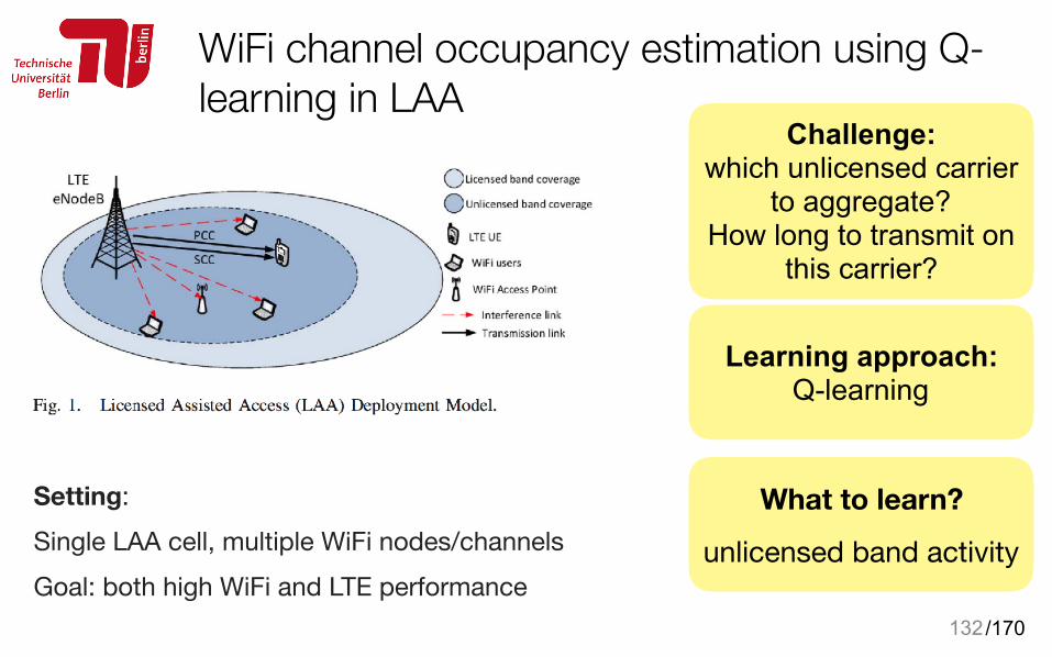
Setting:Single LAA cell, multiple WiFi nodes/channelsGoal: both high WiFi and LTE performance
132
Challenge: which unlicensed carrier
to aggregate? How long to transmit on
this carrier?
Learning approach: Q-learning
What to learn?
unlicensed band activity
/170
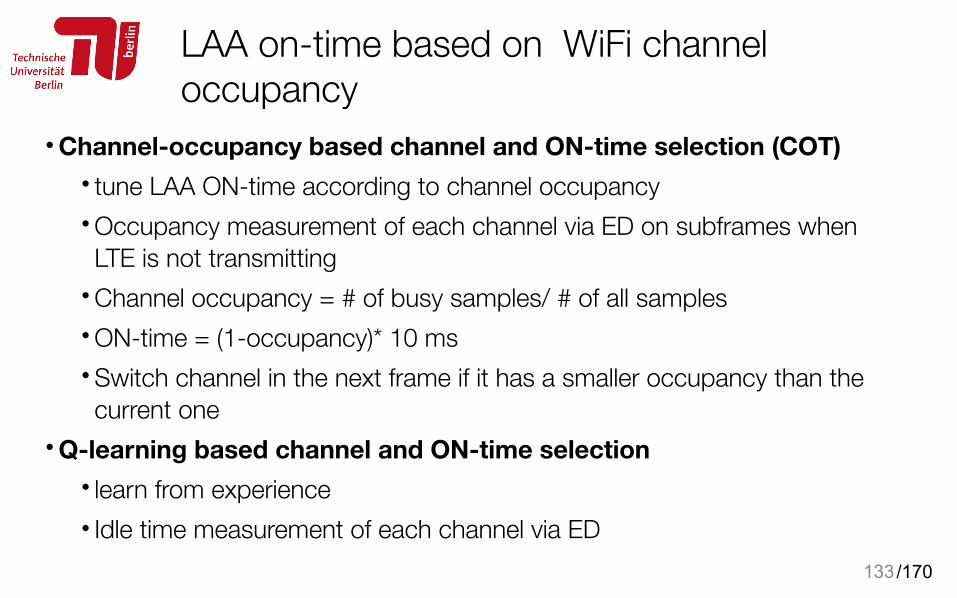
LAA on-time based on WiFi channel occupancy
• Channel-occupancy based channel and ON-time selection (COT) • tune LAA ON-time according to channel occupancy • Occupancy measurement of each channel via ED on subframes when LTE is not transmitting
• Channel occupancy = # of busy samples/ # of all samples • ON-time = (1-occupancy)* 10 ms • Switch channel in the next frame if it has a smaller occupancy than the current one
• Q-learning based channel and ON-time selection • learn from experience • Idle time measurement of each channel via ED
133
/170
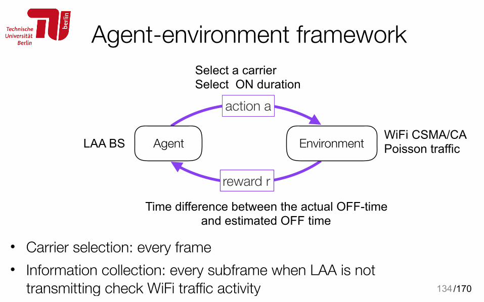
Agent-environment framework
• Carrier selection: every frame • Information collection: every subframe when LAA is not
transmitting check WiFi traffic activity 134
action a
reward r
AgentLAA BS Environment WiFi CSMA/CA Poisson traffic
Select a carrier Select ON duration
Time difference between the actual OFF-time and estimated OFF time
/170
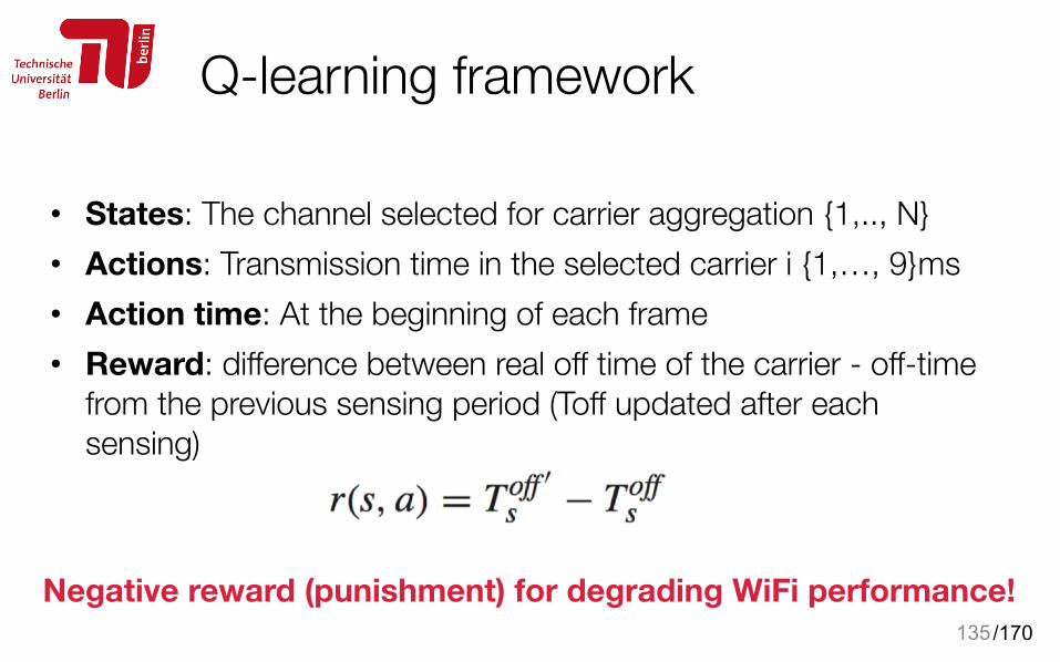
Q-learning framework
• States: The channel selected for carrier aggregation {1,.., N} • Actions: Transmission time in the selected carrier i {1,…, 9}ms • Action time: At the beginning of each frame • Reward: difference between real off time of the carrier - off-time
from the previous sensing period (Toff updated after each sensing)
135
Negative reward (punishment) for degrading WiFi performance!

/170
Q-value initial value and update rule
• Optimal action (a: LAA transmission duration) depends on the selected channel’s availability time
136
Select a channel with low occupancy (high off duration)
Select transmission time matching the channel off time
Only immediate reward, discount factor = 0
/170
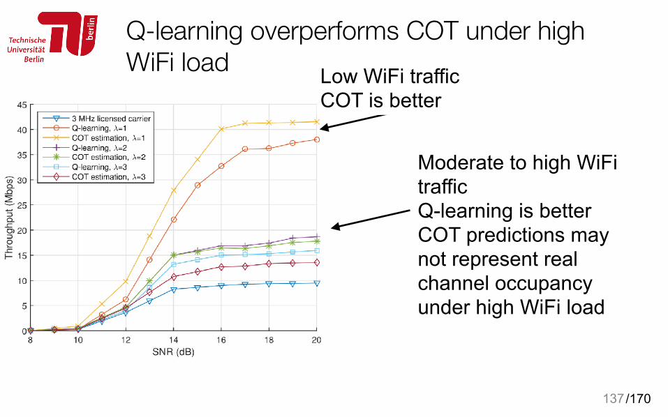
Q-learning overperforms COT under high WiFi load
137
Moderate to high WiFi traffic Q-learning is better COT predictions may not represent real channel occupancy under high WiFi load
Low WiFi traffic COT is better
/170
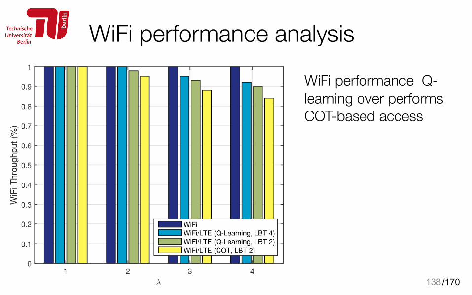
WiFi performance analysis
WiFi performance Q-learning over performs COT-based access
138
/170139
Case study #4 Can WiFi exploit ML for protecting itself from LTE
interference?
yes, WiPLUS!
Olbrich, M., Zubow, A., Zehl, S. and Wolisz, A. "WiPLUS: Towards LTE-U Interference Detection, Assessment and Mitigation in 802.11 Networks", in European Wireless 2017 (EW2017), Best Paper Award, May, 2017.
LTE
/170
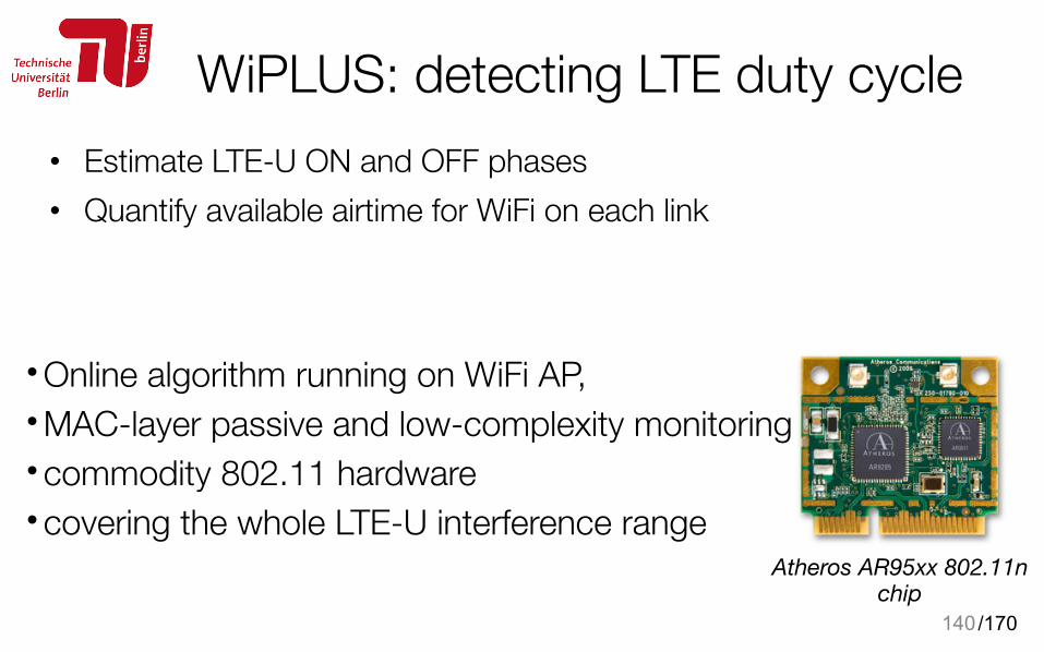
WiPLUS: detecting LTE duty cycle• Estimate LTE-U ON and OFF phases • Quantify available airtime for WiFi on each link
140
Atheros AR95xx 802.11n chip
• Online algorithm running on WiFi AP, • MAC-layer passive and low-complexity monitoring • commodity 802.11 hardware • covering the whole LTE-U interference range
/170
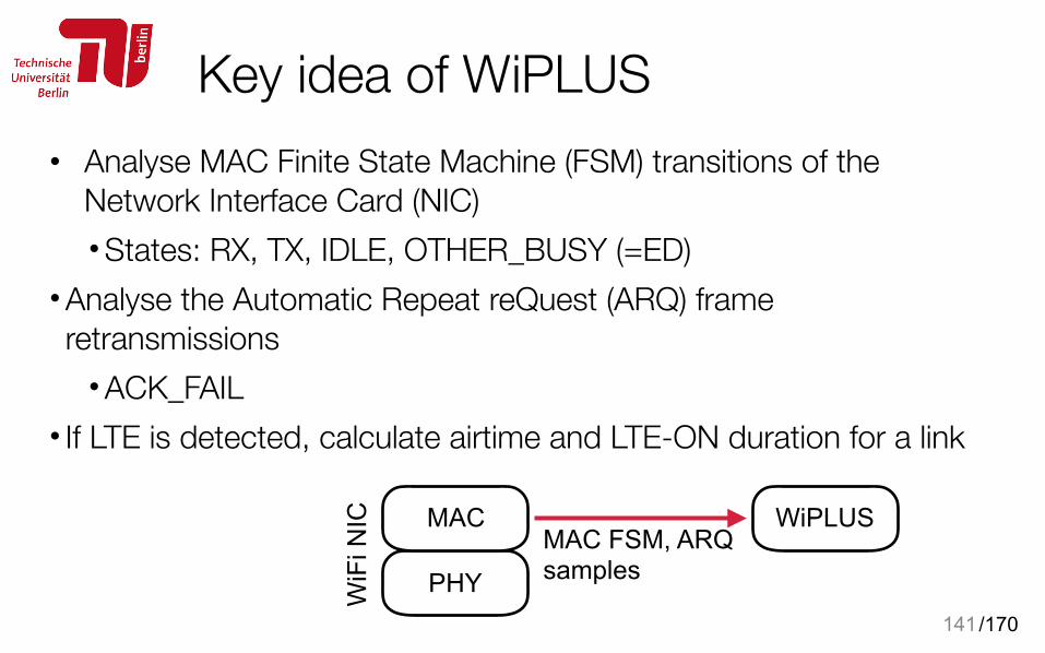
Key idea of WiPLUS• Analyse MAC Finite State Machine (FSM) transitions of the
Network Interface Card (NIC) • States: RX, TX, IDLE, OTHER_BUSY (=ED)
• Analyse the Automatic Repeat reQuest (ARQ) frame retransmissions
• ACK_FAIL • If LTE is detected, calculate airtime and LTE-ON duration for a link
141
PHY
MAC WiPLUSMAC FSM, ARQ samples
WiF
i NIC
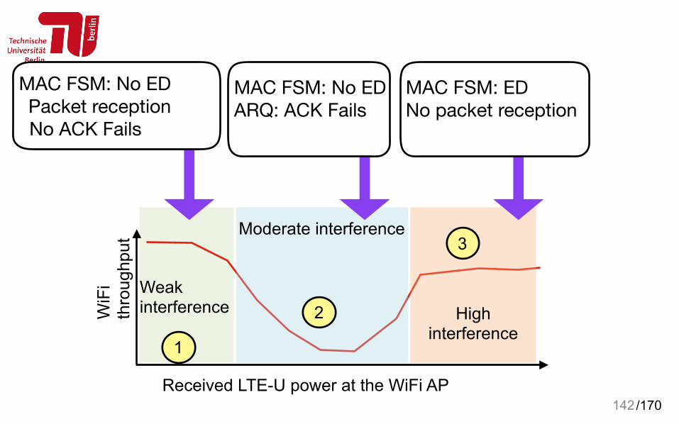
/170142Received LTE-U power at the WiFi AP
Moderate interference
High interference
Weak interferenceW
iFi
thro
ughp
ut
1
2
3
MAC FSM: No ED Packet reception No ACK Fails
MAC FSM: No EDARQ: ACK Fails
MAC FSM: EDNo packet reception
/170143Received LTE-U power at the WiFi AP
Moderate interference
High interference
Weak interferenceW
iFi
thro
ughp
ut
1
2
3
MAC FSM: No ED Packet reception No ACK Fails
MAC FSM: No EDARQ: ACK Fails
MAC FSM: EDNo packet reception
LTE ON time
/170
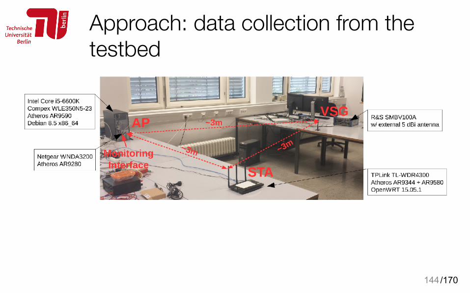
Approach: data collection from the testbed
144
/170
ML approach: data analysis Data: • data collection via periodic samples from the NIC • Fraction of time in each MAC-state, ARQ number of
packet retransmissions during the respected sampling
145
Raw data
More useful representation Rt which represents (possible) LTE ON-time
total MAC time spent in transmission in the sampling period
/170
K-means clustering to detect the clusters of transmission duration and clean the outliers
146
WiPLUS Detector Pipeline • Input data is very noisy, • Detector pipeline:
– Periodically sampled MAC FSM states (RX/TX/IDLE/ED state) + MAC ARQ states (missing ACK),
– Spurious signal extraction (cleansing),
– FFT / PWM signal detection, – Used to find fundamental
frequency (harmonics) of interfering signal,
– ML cluster detection (k-means): • Remove signals outside clusters to
suppress outliers, – Low pass filtering, – LTE-U ON time estimation &
calculation of eff. available airtime for WiFi.
Read MAC state & ARQ info
Spurious signal extraction
Enough samples?
FFT
CCI(f)
PWM signal detection
Periodic spectrum?
fPWM
Cluster detection
CCI(t)
Low pass FIR filter
CCI‘(t)
LTE-U ON time estimation
Estimation of eff. medium airtime
TON
TON=0
NO
NO YES
YES
CCI‘(t)~
WiPLUS detector pipeline R
x x
/170
WiPLUS protoype
147
• WiPLUS can estimate airtime quite accurately! (RMS < 3% for DL) • Possible use of this capability: select channel based on observed LTE
activity • Python’s Scikit-learn
Simple detector: Only ED
/170
Case study #5 WiFi performance estimation
148Herzen, Julien, Henrik Lundgren, and Nidhi Hegde. "Learning Wi-Fi performance." IEEE SECON 2015
Regression
AP 2 AP 3AP 1
/170
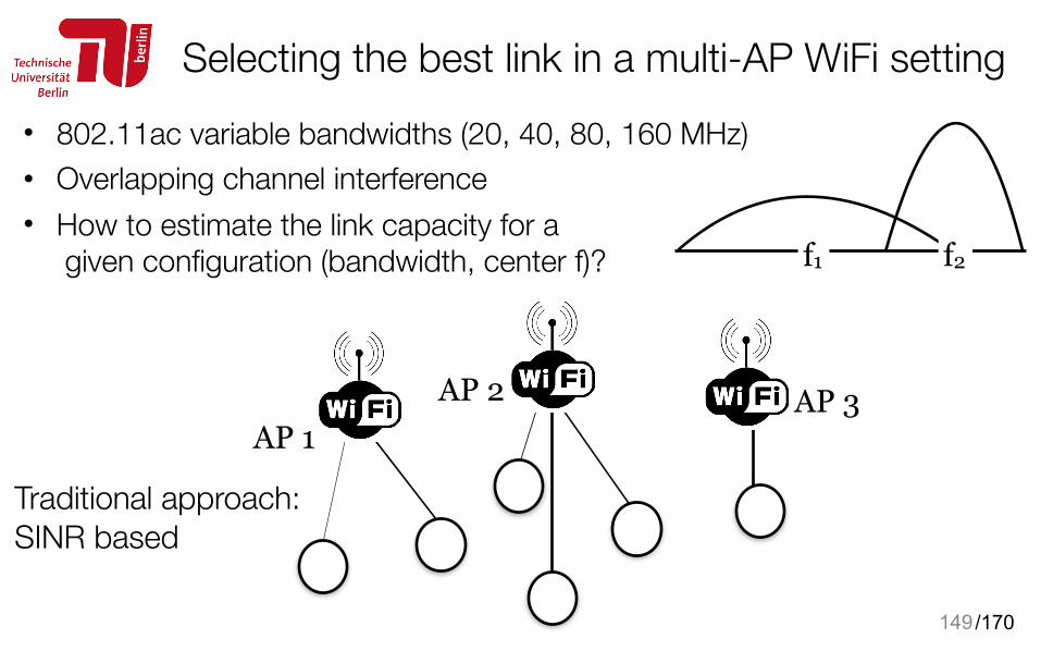
• 802.11ac variable bandwidths (20, 40, 80, 160 MHz) • Overlapping channel interference • How to estimate the link capacity for a
given configuration (bandwidth, center f)?
Selecting the best link in a multi-AP WiFi setting
149
f1 f2
AP 1AP 2 AP 3
Traditional approach: SINR based
/170
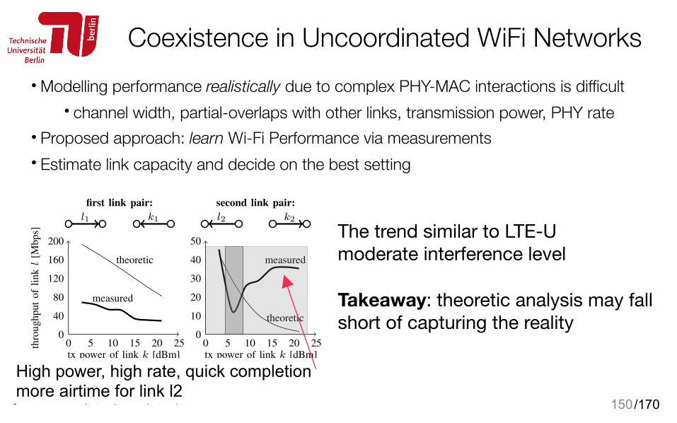
Coexistence in Uncoordinated WiFi Networks• Modelling performance realistically due to complex PHY-MAC interactions is difficult
• channel width, partial-overlaps with other links, transmission power, PHY rate • Proposed approach: learn Wi-Fi Performance via measurements • Estimate link capacity and decide on the best setting
150
0 5 10 15 20 250
40
80
120
160
200
tx power of link k [dBm]
thro
ughput
of
linkl
[Mb
ps]
measured
theoretic
0 5 10 15 20 250
10
20
30
40
50
tx power of link k [dBm]
measured
theoretic
l1 k1
first link pair:
l2 k2
second link pair:
Figure 2: Measured throughput and theoretical capacity of l, whenk varies its transmit power. The results are shown for two differentpairs of links (l1, k1) and (l2, k2) from our testbed.
performance in three distinct regimes (represented by threeshaded regions in the figure). When k’s transmit power is low,the links are nearly independent and l suffers little interferencefrom k. When k’s transmit power grows to intermediate values,k starts interfering with l. In this case, l carrier-senses k, andinterference mitigation is done in time-domain via CSMA/CA.However, a closer inspection of packets reveals that k itself
does not have a good channel quality (as it uses only anintermediate transmit power), which forces it to use relativelyrobust (and slow) modulations. As a result, in this intermediateregime, k consumes a significant portion of the time to transmitits packets, which reduces l’s throughput (due to the rate-anomaly). Finally, when k uses a large transmit power, it alsouses faster modulations, which has the apparently paradoxicaleffect of increasing l’s throughput.
In this second example, the information-theoretic formu-lation for the capacity does not capture all these “802.11-specific” cross-layer and multi-modal effects. Instead, it showsa monotonic dependency on transmit power, because it treatsthe case of Gaussian channels subject to constant and whitenoise interference.In fact, in the cases where a time-sharingscheme such as CSMA/CA is employed, links often have theopportunity to transmit alone on the channel, thus withoutobserving any interference at all during their transmission1.
It is thus clear that even in such a simple setting, a resourceallocation algorithm relying on monotonic expressions of theSINR is likely to take bad decisions. Despite these problems– and despite the fact that SINR models are usually notconsidered strong predictors of wireless performance – thesemodels are still the models of choice for allocating resources atthe PHY layer, due to their generality: By adapting judiciouslythe power values in the SINR Equation (2), it is possible touse variable transmit powers (as we just did), but also partiallyoverlapping channels [23] and variable bandwidths [26] asinputs of SINR models. In addition, a large body of literatureon optimal resource allocation also relies on SINR modelsin various contexts [3], [10], [15], [19], [22]. By contrast,MAC layer models such as Bianchi’s are often accurate withhomogeneous PHY configurations, but cannot be used to
1This is also the reason the actual throughput might be largely above thepredicted capacity.
capture such heterogeneous PHY configurations.
III. LEARNING PERFORMANCE MODELS
A. Approach
A natural step to improve the accuracy of SINR-basedmodels is to seed (or fit) some parameters (for instance, afactor controlling the magnitude of the prediction) to theobservations of actual measurements. The approach of seedinga model with measurements can be appropriate for networkswith collaborative APs, such as enterprise networks, and it hasbeen taken in [21], [26], [27] and others (see Section VII fora discussion). We now show that, if one has the possibility ofconducting an initial measurement phase, then it is possible todirectly learn the model itself from the data, instead of fittingor seeding a previously existing model. Our overall approachconsists of the three following steps.
1) Measurement phase: This phase consists in performingN short-duration controlled experiments. Considering againthe black box representation of Figure 1 (although generalizedfor several links), each experiment consists in measuring thethroughput of a given link l, for one particular combination ofinputs (which we call features). This phase is relatively short;we observe in Section IV-D that it is possible to “learn” ourentire indoor testbed with reasonable accuracy in less than 6hours.2) Learning phase: Once the measurements are obtained,this phase consists in finding a mathematical function thatmaps the features to observed throughputs. This functionshould approximate the throughput well on the measured datapoints. However, to be useful, it must not overfit existingmeasurements, which are intrinsically noisy. Instead, it shouldgeneralize to unseen combinations of input features (whichcan potentially relate to unseen nodes and links). Supervisedmachine learning provides us with precisely the tools to handlethis challenge.3) Black box representation: Once a good function has beenfound, we can discard the measurements and use the functionitself to cheaply compute throughput predictions. Such blackboxes can then be used by the APs themselves for selectingefficient configurations (e.g., with predicted throughputs satis-fying traffic demands) without probing.
Importantly, we observe in Section IV-C that learned modelscontinue to be useful in new or unseen environments, and thatthe training procedure does not need to be repeated when newwireless links come and go. We detail our procedure in theremainder of this section.
B. Feature Selection
Consider a link l, for which we want to predict saturatedthroughput (i.e., under saturated traffic load2) for arbitraryspectrum and transmit power configurations, given a set Nl ofK neighboring links with arbitrary conditions, configurations
2We target saturated throughput because it is the maximum achievablethroughput in a given configuration. In particular, we assume that if throughputt is achievable, then any throughput t′ < t is also achievable.
The trend similar to LTE-U moderate interference level
Takeaway: theoretic analysis may fall short of capturing the reality
High power, high rate, quick completion more airtime for link l2
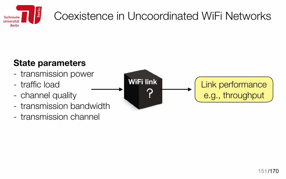
/170
Coexistence in Uncoordinated WiFi Networks
151
State parameters - transmission power - traffic load - channel quality - transmission bandwidth - transmission channel
Link performance e.g., throughput
WiFi link
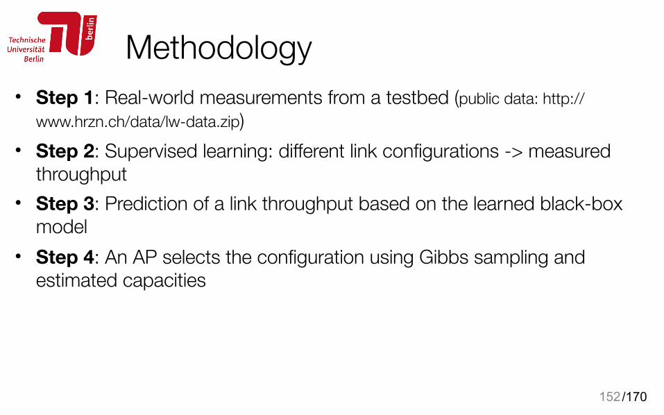
/170
Methodology• Step 1: Real-world measurements from a testbed (public data: http://
www.hrzn.ch/data/lw-data.zip) • Step 2: Supervised learning: different link configurations -> measured
throughput • Step 3: Prediction of a link throughput based on the learned black-box
model • Step 4: An AP selects the configuration using Gibbs sampling and
estimated capacities
152
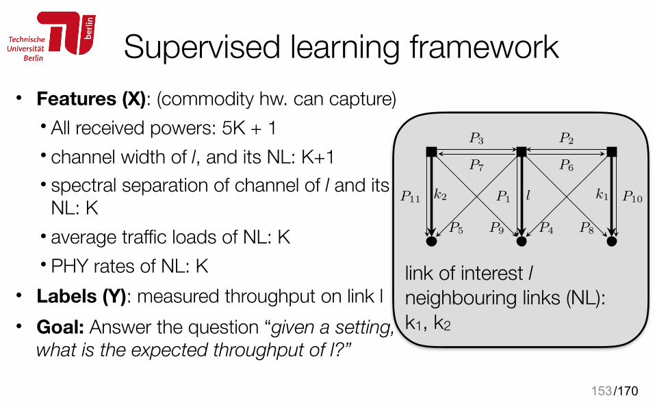
/170
Supervised learning framework• Features (X): (commodity hw. can capture)
• All received powers: 5K + 1 • channel width of l, and its NL: K+1 • spectral separation of channel of l and its
NL: K • average traffic loads of NL: K • PHY rates of NL: K
• Labels (Y): measured throughput on link l • Goal: Answer the question “given a setting,
what is the expected throughput of l?”
153
l k1k2
P6
P2
P1
P4
P10
P8
P7
P3
P9
P11
P5
Figure 3: Throughput prediction setting for a link l and twoneighboring links Nl = {k1, k2}. We wish to predict the throughputthat l could potentially obtain, given the various received powersP1, . . . , P11, as well as the physical rates, channel widths, centerfrequencies, and traffic loads of k1 and k2.
and traffic demands. Such a scenario is shown in Figure 3for K = 2. The features must include factors that impactthe performance and are measurable by the transmitter of land its immediate neighbors. We selected the following list offeatures, because it is known that they all have an immediateimpact on performance [4], [5], [11], [23]:
• The power received by each node of l from every trans-mitting node, and the power received by every other node,from the transmitter of l. These quantities are denotedP1, . . . , P11 in Figure 3 (assuming downlink traffic, fromthe APs to their clients). They depend on the transmitpowers and the various channel gains, and they can beeasily measured online by commodity hardware using RSSI(received signal strength indicator). There are 5K +1 suchpower quantities in general.
• The channel widths used by l and by the links in Nl. Thereare K + 1 such values.
• The spectral separations between the center frequency usedby l, and the center frequencies used by all the other linksin Nl. There are K such values.
• The K average traffic loads of the links in Nl.• The physical rates (determined by the 802.11n MCS index)
used on each link in Nl. There are again K such values.
Adding up the above-mentioned features, we have access tod := 9K + 2 quantities to estimate the throughput that l canobtain in the presence of K interferers. Note that this listof features is not an exhaustive list of the factors affectingperformance that can be known or measured by the APs. Forinstance, we could make it more complete by including thepacket sizes, higher order statistics to describe the traffic loadsof interferers (instead of the mean only), or more detailedPHY layer information (e.g., capturing multipath effects orfrequency-selective fading). Including more features couldfurther increase the predictive power and generality of thelearned models. However, the features selected here alreadyallow us to build useful models, while having the advantageof being simple and easy to acquire with commodity hardware.
C. Measurement Phase
The initial measurement phase consists of N measurementswith different combinations of features. Some of the featurescan be directly controlled (namely, the channel widths, spectralseparations and traffic loads) and others cannot (the receivedpowers depend both on the transmit powers and channel gains,
and the physical rates depend on the auto-rate mechanismused by the APs). Each of the N measurements consists oftwo sub-experiments. We first perform an experiment duringwhich l is silent, in order to obtain a corresponding vectorx ∈ Rd of features (some of which are controlled, othersare measured). We then repeat the experiment with l sendingsaturated traffic, and measure its throughput tl. Our goal is toexpose the learning procedure to as wide a variety of situationsas possible. To this end, we apply the following samplingprocedure for each of the N data points.
We start by selecting a link l uniformly at random amongall the links formed by all the nodes of the network. Wethen sample K random interfering links, where K itself israndomly drawn between 0 and max K, and max K denotesa fixed upper bound on K. For l and the K links in Nl, wesample transmit powers and spectral configurations uniformlyat random from the set of configurations that do produce someinterference (i.e., such that each link in Nl uses a band at leastadjacent or partially overlapping with l). Finally, for each linkk in Nl, we sample a traffic load in the interval (0, h(wk)/K],where h(wk) is a value representing the maximum throughputachievable on an isolated link using bandwidth wk. We takeh(20 MHz) = 80 Mbps and h(40 MHz) = 130 Mbps inour training procedure, in line with the maximum achievablethroughput of our 802.11n cards. Our goal is to predictperformance for arbitrary interfering loads, and sampling theloads in this way allows us to expose the learning procedure todifferent environments with both light and heavy contention.In particular, we measured that the offered loads of the nodesin Nl was above capacity (i.e., saturated) in about 54% of theexperiments (mainly due to inter-neighbors interference). Theremaining experiments consist of non-saturated conditions.
Once the configurations have been chosen, we performthe first experiment with only the K interfering links active.During this experiment, we measure the average physical ratesused by each of the K links in Nl, and we group all the above-mentioned features in a vector xi. In order to vary K between0 and max K but keep features vectors of fixed dimensiond, we append 9 · (max K − K) default “flag” values to xi,using −110 dBm for all the power values, and setting allthe remaining features to zero3. We then perform the secondexperiment in the same conditions, but with link l sendingsaturated traffic, and we measure its achieved throughput. Eachof the two sub-experiments constituting each of the N datapoints needs only to last a few seconds (in order to measurephysical rates and throughput), and the whole procedure iseasily automated.
D. Learning
Let us write {(x1, t1), . . . , (xN , tN )} ⊂ Rd ×R for our setof measurements. Our goal is now to find a function f : Rd →R that maps xi to a value close to ti for each measurement i.Learning the function f from the observed data is a regression
3The current number of interfering links K is thus an implicit feature,encoded by the presence/absence of flag values.
link of interest l neighbouring links (NL): k1, k2
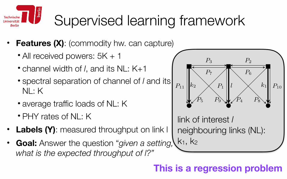
/170
Supervised learning framework• Features (X): (commodity hw. can capture)
• All received powers: 5K + 1 • channel width of l, and its NL: K+1 • spectral separation of channel of l and its
NL: K • average traffic loads of NL: K • PHY rates of NL: K
• Labels (Y): measured throughput on link l • Goal: Answer the question “given a setting,
what is the expected throughput of l?”
154
l k1k2
P6
P2
P1
P4
P10
P8
P7
P3
P9
P11
P5
Figure 3: Throughput prediction setting for a link l and twoneighboring links Nl = {k1, k2}. We wish to predict the throughputthat l could potentially obtain, given the various received powersP1, . . . , P11, as well as the physical rates, channel widths, centerfrequencies, and traffic loads of k1 and k2.
and traffic demands. Such a scenario is shown in Figure 3for K = 2. The features must include factors that impactthe performance and are measurable by the transmitter of land its immediate neighbors. We selected the following list offeatures, because it is known that they all have an immediateimpact on performance [4], [5], [11], [23]:
• The power received by each node of l from every trans-mitting node, and the power received by every other node,from the transmitter of l. These quantities are denotedP1, . . . , P11 in Figure 3 (assuming downlink traffic, fromthe APs to their clients). They depend on the transmitpowers and the various channel gains, and they can beeasily measured online by commodity hardware using RSSI(received signal strength indicator). There are 5K +1 suchpower quantities in general.
• The channel widths used by l and by the links in Nl. Thereare K + 1 such values.
• The spectral separations between the center frequency usedby l, and the center frequencies used by all the other linksin Nl. There are K such values.
• The K average traffic loads of the links in Nl.• The physical rates (determined by the 802.11n MCS index)
used on each link in Nl. There are again K such values.
Adding up the above-mentioned features, we have access tod := 9K + 2 quantities to estimate the throughput that l canobtain in the presence of K interferers. Note that this listof features is not an exhaustive list of the factors affectingperformance that can be known or measured by the APs. Forinstance, we could make it more complete by including thepacket sizes, higher order statistics to describe the traffic loadsof interferers (instead of the mean only), or more detailedPHY layer information (e.g., capturing multipath effects orfrequency-selective fading). Including more features couldfurther increase the predictive power and generality of thelearned models. However, the features selected here alreadyallow us to build useful models, while having the advantageof being simple and easy to acquire with commodity hardware.
C. Measurement Phase
The initial measurement phase consists of N measurementswith different combinations of features. Some of the featurescan be directly controlled (namely, the channel widths, spectralseparations and traffic loads) and others cannot (the receivedpowers depend both on the transmit powers and channel gains,
and the physical rates depend on the auto-rate mechanismused by the APs). Each of the N measurements consists oftwo sub-experiments. We first perform an experiment duringwhich l is silent, in order to obtain a corresponding vectorx ∈ Rd of features (some of which are controlled, othersare measured). We then repeat the experiment with l sendingsaturated traffic, and measure its throughput tl. Our goal is toexpose the learning procedure to as wide a variety of situationsas possible. To this end, we apply the following samplingprocedure for each of the N data points.
We start by selecting a link l uniformly at random amongall the links formed by all the nodes of the network. Wethen sample K random interfering links, where K itself israndomly drawn between 0 and max K, and max K denotesa fixed upper bound on K. For l and the K links in Nl, wesample transmit powers and spectral configurations uniformlyat random from the set of configurations that do produce someinterference (i.e., such that each link in Nl uses a band at leastadjacent or partially overlapping with l). Finally, for each linkk in Nl, we sample a traffic load in the interval (0, h(wk)/K],where h(wk) is a value representing the maximum throughputachievable on an isolated link using bandwidth wk. We takeh(20 MHz) = 80 Mbps and h(40 MHz) = 130 Mbps inour training procedure, in line with the maximum achievablethroughput of our 802.11n cards. Our goal is to predictperformance for arbitrary interfering loads, and sampling theloads in this way allows us to expose the learning procedure todifferent environments with both light and heavy contention.In particular, we measured that the offered loads of the nodesin Nl was above capacity (i.e., saturated) in about 54% of theexperiments (mainly due to inter-neighbors interference). Theremaining experiments consist of non-saturated conditions.
Once the configurations have been chosen, we performthe first experiment with only the K interfering links active.During this experiment, we measure the average physical ratesused by each of the K links in Nl, and we group all the above-mentioned features in a vector xi. In order to vary K between0 and max K but keep features vectors of fixed dimensiond, we append 9 · (max K − K) default “flag” values to xi,using −110 dBm for all the power values, and setting allthe remaining features to zero3. We then perform the secondexperiment in the same conditions, but with link l sendingsaturated traffic, and we measure its achieved throughput. Eachof the two sub-experiments constituting each of the N datapoints needs only to last a few seconds (in order to measurephysical rates and throughput), and the whole procedure iseasily automated.
D. Learning
Let us write {(x1, t1), . . . , (xN , tN )} ⊂ Rd ×R for our setof measurements. Our goal is now to find a function f : Rd →R that maps xi to a value close to ti for each measurement i.Learning the function f from the observed data is a regression
3The current number of interfering links K is thus an implicit feature,encoded by the presence/absence of flag values.
link of interest l neighbouring links (NL): k1, k2
This is a regression problem
/170
Used tools for this regression problem
• Regression tree, Gradient Boosted Regression Trees (GBRT), Support Vector Regression (SVR)
• Comparison baseline: SINR-based model • accuracy of predictions: coefficient of determination R2, RMSE
• Python scikit-learn package • 50-fold cross-validation
155
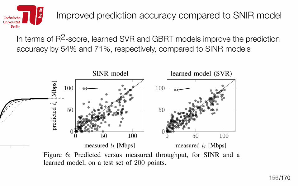
/170
Improved prediction accuracy compared to SNIR model
In terms of R2-score, learned SVR and GBRT models improve the prediction accuracy by 54% and 71%, respectively, compared to SINR models
156
(a) (b)
SINR regr.tree
SVR GBRT
0.4
0.6
0.8
R2-s
core
R2-score
10
15
20
25
roo
tm
ean
-sq
uar
eder
ror
(RM
SE
)RMSE
−40 −20 0 20 400
0.2
0.4
0.6
0.8
1
prediction error [Mbps]
pro
port
ion
of
exper
imen
ts
mean learned (SVR)
SINR learned (GBRT)
.
Figure 5: Summary of prediction performance for various models (a)and empirical CDF of prediction errors (b). The “mean” model inplot (b) represents the errors obtained by a baseline predictor thatalways predicts the mean throughput of the training set.
we recall, are the only known class of models capturingphenomena such as overlapping channels). In terms of errordistribution, 90% of the errors made by learned models arebetween −25 Mbps and 25 Mbps, whereas 90% of the errorsmade by SINR-based models are between −35 Mbps and36 Mbps. The fact that learned models are more accurateis remarkable; it demonstrates that, as far as performanceprediction is concerned, learning abstract models coming fromthe machine learning domain can be much more efficient thantrying to fit (or seed) pre-existing specialized models.
In order to visualize the actual predictions in detail, wealso show a scatter plot of the throughputs predicted by SINRmodels and learned SVR models, against the actual measuredthroughputs, in Figure 6. Clearly, SVR models perform muchbetter and produce fewer outlying predictions than SINRmodels. Note that obtaining perfect predictions is impossiblehere, considering the fact that both the measured features andthe throughput are highly noisy variables, measured with com-modity hardware. To illustrate this, we examine in more detailthe features corresponding to the worst prediction obtained byboth models (shown by an arrow on the plots – incidentally,this is the same point for both models). This point correspondsto a link l subject to no (controlled) interference (i.e., K = 0),with an apparently good channel quality (the measured RSSIis -59 dBm), and using a bandwidth of 40 MHz, supposedlyyielding the largest capacity. Yet, despite these features, themeasured throughput was low. We can only speculate aboutthe causes for this discrepancy (it may be due to especiallyhigh noise or software factors). In any case, this exampleillustrates the limits of throughput predictability with imperfectinformation.
C. Generalization
Due to the evaluation on test set, the previous results addresscases where predictions are produced for unseen combinationsof features. We now attempt to push our models further, bypredicting throughputs for unknown links, potentially belong-ing to different environments.
1) Predictions for Unknown Links: For each possible linkl, we remove both l and its reverse link (obtained by invertingthe transmitter and the receiver of l) from the training set. We
SINR model learned model (SVR)
0 50 1000
50
100
measured tl [Mbps]
pre
dic
tedt̂ l
[Mbps]
0 50 1000
50
100
measured tl [Mbps]
Figure 6: Predicted versus measured throughput, for SINR and alearned model, on a test set of 200 points.
then predict throughput for each data point that contains l (orits reverse link), and show the results in Figure 7. Comparedwith Figure 5(a), some models (especially the ones based onregression trees) see their accuracy slightly decreased. How-ever, the models learned with SVR still perform remarkablywell; in terms of R2-score, their accuracy is reduced by lessthan 4%, and they still improve the accuracy by 49% comparedto SINR-based models.
2) Different Environments: We now manually divide thelinks present in our trace in three distinct categories, dependingon the type of attenuation that they experience. The categoriesare shown in Figure 4, and they correspond to the followinglink division: (i) links that traverse mostly empty space, (ii)links that traverse sparsely spaced walls and (iii) links thattraverse densely spaced walls.
For each category, we remove all the links (and their reverse)belonging to this category from the training set. We then buildthe test set so as to predict throughput for links belongingonly to this category. The goal of this experiment is to testprediction accuracy in the worst possible conditions: eachmodel is learned on links that operate in conditions radicallydifferent than the conditions prevailing during the actualpredictions. In addition to the three link categories (i)-(iii), wealso split our testbed in two halves A and B (also shown inFigure 4). The resulting accuracies are shown in Figure 8. Evenin these difficult cases, the learned models based on SVR showa graceful degradation and keep a relatively high accuracy(with R2-scores always larger than 0.54). When predicting onhalf B with models learned on half A, models based on SVReven obtain similar accuracies as when learning using the fulltestbed. This allows us to draw some conclusions on the extentto which our method generalizes. Even when learning modelson a different part of the testbed, or using radically differentlinks, abstract models based on machine learning still havefar more predictive power than measurement-seeded modelsbased on SINR.
D. How Much Learning is Needed?
Finally, we measure the accuracy as a function of thetraining set size N . For different N , we learn models usingN experiments sampled at random from our experiment trace.We then predict the throughput for all the other experiments,and measure the R2-score. The results are shown in Figure 9.Using N = 100 training experiments is enough to obtainbetter accuracy than SINR models, and N = 1000 experiments
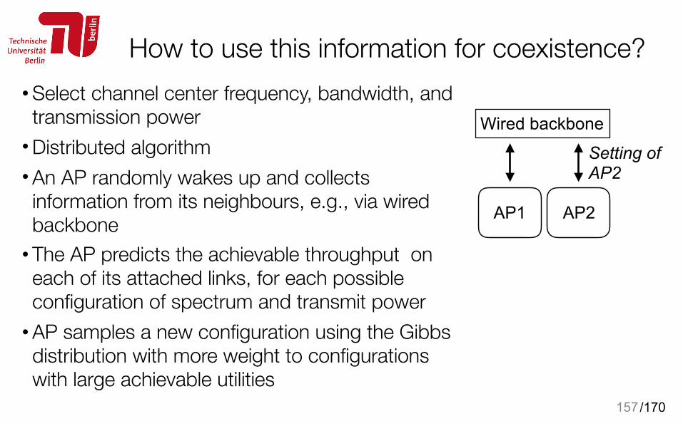
/170
How to use this information for coexistence?• Select channel center frequency, bandwidth, and transmission power
• Distributed algorithm • An AP randomly wakes up and collects information from its neighbours, e.g., via wired backbone
• The AP predicts the achievable throughput on each of its attached links, for each possible configuration of spectrum and transmit power
• AP samples a new configuration using the Gibbs distribution with more weight to configurations with large achievable utilities
157
AP1 AP2
Wired backbone
Setting of AP2
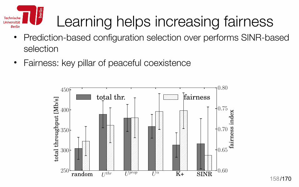
/170
Learning helps increasing fairness• Prediction-based configuration selection over performs SINR-based
selection • Fairness: key pillar of peaceful coexistence
158random Uthr Uprop Uα K+ SINR
250
300
350
400
450
tota
lth
rou
gh
pu
t[M
b/s
] total thr.
0.60
0.65
0.70
0.75
0.80
fair
nes
sin
dex
fairness
Figure 10: Throughput and fairness for differentutility functions. We also show the results for ran-dom configurations, the ”K+” algorithm, and ouralgorithm with U thr , but using the measurement-seeded SINR model instead of a learned model.
0 5 10 15 20transmit power [dBm]
0.0
0.2
0.4
0.6
0.8
1.0
pro
por
tion
sele
cted
Uthr
Uprop
Uα
Figure 11: CDF of transmit powersselected with different utilities andsampling policies. Fair policies se-lect lower transmit powers.
10-20 20-30 30-40 40-50 50-60 60-70 70-80 all 100load [Mb/s]
0.4
0.5
0.6
0.7
0.8
0.9
pro
por
tion
of4
0M
Hz
sele
cted
width
10
12
14
16
18
20
aver
age
tra
nsm
itp
ower
[dB
m]
power
Figure 12: Proportion of time a bandwidth of 40MHz is selected, and selected transmit power, asa function of traffic load. Efficient load balanc-ing is achieved, as heavily loaded APs samplewider bandwidths and larger transmit powers.
802.11 networks. [26] runs the spectrum allocation jointly withscheduling decisions at a central controller, and [17] proposesa distributed algorithm for the joint allocation of center fre-quencies and bandwidths. None of these algorithms considersthe transmit power, and they do not adapt to various utilityfunctions. Our learned models predict achievable throughputs,which can be directly plugged into the utility maximizationframework. This removes the need to use indirect optimizationobjectives (such as minimization of interference, which oftendoes not coincide with performance maximization [17]).
The theoretical works that are the closest to ours are [3],[15]. These papers propose optimal algorithms for channeland/or power selection, but do not consider channel width.Further, they have not been implemented in real networks.
VIII. CONCLUSIONS
We investigated and validated a new approach for predictingthe performance of Wi-Fi networks. Rather than manuallyfitting complex models to capture complex dependencies,we showed that it is possible to directly learn the modelsthemselves, from a limited set of observed measurements. Thisapproach bypasses the usual modeling process, which requiresboth deep knowledge and tedious analysis, and yet often yieldsmodels that are either too restricted or too inaccurate. Weobserved that abstract black box models built using supervisedmachine learning techniques – without any deep knowledge ofthe complex interference dynamics of 802.11 networks – canlargely outperform the dominant class of SINR-based models.Further, we have shown that these models still work whenthey have to predict performance for links that have neverbeen observed during the learning phase.
We have used one such model as an oracle in a newdistributed utility-optimal resource allocation algorithm. Weobserved that our algorithm adapts well to various optimiza-tion criteria, and that our learned model is instrumental forachieving good performance in these tangled settings.
REFERENCES
[1] G. Bianchi. Performance analysis of the ieee 802.11 distributedcoordination function. IEEE JSAC, 2000.
[2] C. M. Bishop. Pattern Recognition and Machine Learning. Springer-Verlag New York, 2006.
[3] S. Borst, M. Markakis, and I. Saniee. Distributed power allocation anduser assignment in OFDMA cellular networks. In Allerton, 2011.
[4] I. Broustis, J. Eriksson, S. V. Krishnamurthy, and M. Faloutsos. Impli-cations of power control in wireless networks: a quantitative study. InPAM, 2007.
[5] R. Chandra, R. Mahajan, T. Moscibroda, R. Raghavendra, and P. Bahl.A case for adapting channel width in wireless networks. In ACMSIGCOMM, 2008.
[6] C. Clancy, J. Hecker, E. Stuntebeck, and T. O’Shea. Applicationsof machine learning to cognitive radio networks. IEEE WirelessCommunications, 2007.
[7] R. C. Daniels and R. Heath. An online learning framework for linkadaptation in wireless networks. In IEEE ITA, 2009.
[8] L. Deek, E. Garcia-Villegas, E. Belding, S.-J. Lee, and K. Almeroth.The impact of channel bonding on 802.11n network management. InACM CoNEXT ’11.
[9] M. Durvy, O. Dousse, and P. Thiran. Modeling the 802.11 protocolunder different capture and sensing capabilities. In INFOCOM, 2007.
[10] R. Etkin, A. Parekh, and D. Tse. Spectrum sharing for unlicensed bands.Selected Areas in Communications, IEEE Journal on, 2007.
[11] M. H. Franck, F. Rousseau, G. Berger-sabbatel, and A. Duda. Perfor-mance anomaly of 802.11b. In IEEE INFOCOM, 2003.
[12] R. Gummadi and H. Balakrishnan. Wireless networks should spreadspectrum based on demands. In ACM HotNets, 2008.
[13] D. Halperin, W. Hu, A. Sheth, and D. Wetherall. Predictable 802.11packet delivery from wireless channel measurements. In SIGCOMM’10.
[14] T. Hastie, R. Tibshirani, and J. Friedman. The elements of statisticallearning: data mining, inference and prediction. Springer, 2008.
[15] N. Hegde and A. Proutiere. Optimal decentralized spectrum sharing: Asimulation approach. In Proc. CISS, Mar. 2012.
[16] J. Herzen, N. Hegde, and H. Lundgren. Learning wi-fi performance(technical report). http://www.hrzn.ch/publications/learning-tr.pdf.
[17] J. Herzen, R. Merz, and P. Thiran. Distributed spectrum assignment forhome wlans. In IEEE INFOCOM, 2013.
[18] A. Kashyap, S. Ganguly, and S. R. Das. A measurement-based approachto modeling link capacity in 802.11-based wireless networks. In ACMMobiCom, 2007.
[19] B. Kauffmann, F. Baccelli, A. Chaintreau, V. Mhatre, K. Papagiannaki,and C. Diot. Measurement-based self organization of interfering 802.11wireless access networks. In IEEE INFOCOM, 2007.
[20] E. Kohler, R. Morris, B. Chen, J. Jannotti, and M. F. Kaashoek. Theclick modular router. ACM Transactions on Computer Systems, 2000.
[21] Y. Li, L. Qiu, Y. Zhang, R. Mahajan, and E. Rozner. Predictableperformance optimization for wireless networks. In SIGCOMM, 2008.
[22] V. Mhatre, K. Papagiannaki, and F. Baccelli. Interference mitigationthrough power control in high density 802.11 WLANs. In IEEEINFOCOM, 2007.
[23] A. Mishra, V. Shrivastava, S. Banerjee, and W. Arbaugh. Partiallyoverlapped channels not considered harmful. In ACM Sigmetrics, 2006.
[24] J. Mo and J. Walrand. Fair end-to-end window-based congestion control.IEEE/ACM Transactions on Networking (ToN), 8(5):556–567, 2000.
[25] L. Qiu, Y. Zhang, F. Wang, M. K. Han, and R. Mahajan. A generalmodel of wireless interference. In ACM MobiCom, 2007.
[26] S. Rayanchu, V. Shrivastava, S. Banerjee, and R. Chandra. FLUID:Improving throughputs in enterprise wireless lans through flexible chan-nelization. In ACM MobiCom, 2011.
[27] C. Reis, R. Mahajan, M. Rodrig, D. Wetherall, and J. Zahorjan.Measurement-based models of delivery and interference in static wire-less networks. In ACM SIGCOMM, 2006.
/170
Selected Literature • Sallent, Oriol, et al. "Learning-based coexistence for LTE operation in unlicensed bands." IEEE ICCW15 • Galanopoulos, Apostolos et al. "Efficient coexistence of LTE with WiFi in the licensed and unlicensed
spectrum aggregation." IEEE TCCN16 • Challita, Ursula, et al. "Proactive resource management in LTE-U systems: A deep learning
perspective." arXiv17 • Cai, Feng'en, et al. "Spectrum sharing for LTE and WiFi coexistence using decision tree and game
theory." IEEE WCNC16 • Rupasinghe, Nadisanka et al. "Reinforcement learning for licensed-assisted access of LTE in the
unlicensed spectrum." IEEE WCNC15 • Jiang, Chunxiao, et al. "Machine learning paradigms for xG wireless networks." IEEE Wcomm,
2017 • Azmat, Freeha et al. "Analysis of spectrum occupancy using machine learning
algorithms." IEEE TVT, 2016 • L. Gavrilovska et al. “Learning and reasoning in CRNs,” IEEE Commun. Surveys Tuts. 2013 • Daniels, Robert C. Machine learning for link adaptation in wireless networks. Diss. 2011. • M.Bkassiny, et. al. "A survey on ML techniques in CRs." IEEE Comm Surveys 2013. 159
/170
Part IV Summary and open research directions
160
5
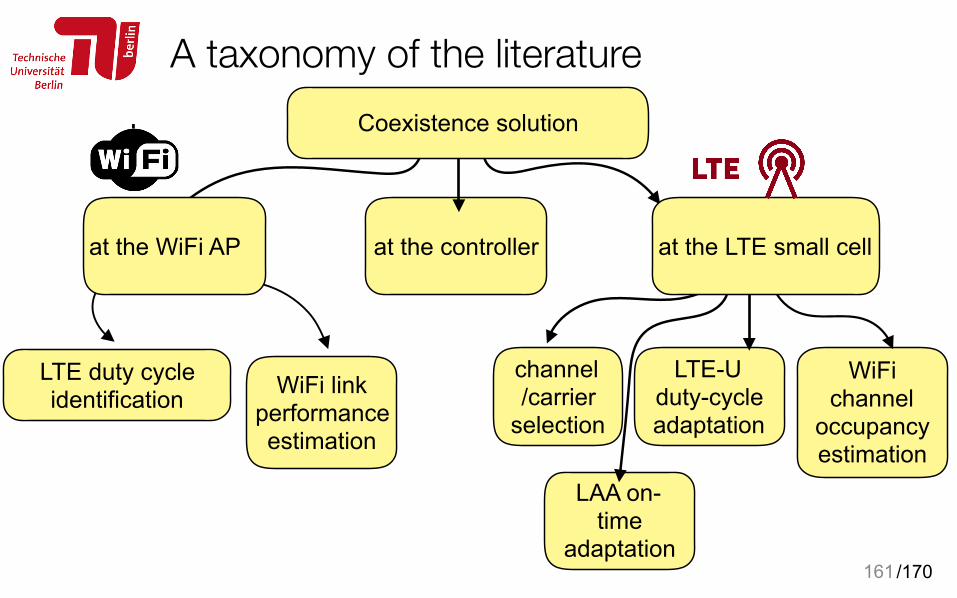
/170
A taxonomy of the literature
161
WiFi link performance estimation
channel /carrier
selection
LTE-U duty-cycle adaptation
WiFi channel
occupancy estimation
at the controller
Coexistence solution
LAA on-time
adaptation
at the LTE small cell
LTE duty cycle identification
at the WiFi AP
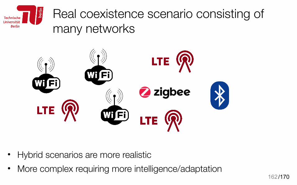
/170
Real coexistence scenario consisting of many networks
• Hybrid scenarios are more realistic • More complex requiring more intelligence/adaptation
162
/170
Desirable properties of coexistence solutions
• standards compliance • soft solutions rather than hardware based • distributed vs centralized/controller based
163
/170
Challenges of applying ML approaches• Feasibility in practical settings
• Complexity • Real-time convergence time • What happens till convergence? • Is it really possible to learn?
• Mobile or other dynamic environments • Where to implement ML?
• AP, nodes, network-core, cloud
164
/170
Challenges for wireless researchers Machine learning requires lots of data to learn useful things
• bad news: researchers mostly are limited in access to such real data • good news: publicly-available data (some better than none) • https://crawdad.cs.dartmouth.edu/
• Limited applicability to computation-limited devices, • bad news: ML requires high resources which are mostly not available in
e.g., embedded devices, IoT devices • good news: ML is very active and searching for smart algorithms with
lower complexity • Fog/Cloud can be exploited for such devices
165• Weka, R, Python

/170
DARPA challenge
• https://www.darpa.mil/news-events/2017-08-11a
166
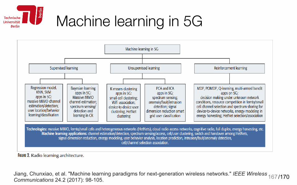
/170
Machine learning in 5G
167Jiang, Chunxiao, et al. "Machine learning paradigms for next-generation wireless networks." IEEE Wireless Communications 24.2 (2017): 98-105.
/170
Summary• The future is unlicensed • Coexistence of such unlicensed networks is a big challenge • ML can provide the capability to embrace uncertainty
168
Thanks!