Chapter 1

Bayesian Methods for

Aircraft Structural Health

Monitoring

T.C. Henderson1, V.J. Mathews1, D.O. Adams1, W.Wang1, S. Nahata1, N. Boonsirisumpun1,A. Joshi1 and E. Grant2

1: University of Utah, Salt Lake City, UT 841122: North Carolina State University, Raleigh, NC 27695

1.1 Introduction

Aircraft structures, whether metallic or composite, are subject to service damagewhich requires their periodic inspection and maintenance. While taking the aircraftout of service is quite costly, the assurance of structural integrity requires suchinspection – and possible repair work based on the inspection results obtained. Ifdamage is detected from an inspection, the decision whether to repair as well asthe method of repair must be made on the basis of data relevant to the specificinspection method being used, and with an uncertainty that has been characterizedas accurately as possible. This is an example of an application that is amenable to aDynamic Data Driven Application System (DDDAS) solution. That is, data can beacquired dynamically, and compared to a model of the structure such that damagecan be located and a determination made as to whether it requires further inspectionand possible repair. Moreover, Bayesian methods allow the characterization ofuncertainty, and with the appropriate inference networks they allow conditionalprobabilities to be determined in terms of what is known about the structure fromthe model and what is measured during the inspection. The methodology underdevelopment allows the accuracy of the model as well as that of the inspection datato be taken into consideration, and uses an iterative approach to improve both themodel and the inspection data. That is, inspection data can be used to determinephysical constants or variables used in the model (e.g., Young’s modulus, diffusionconstants, etc.), and the computational model can be used to improve inspectiondata (e.g., pose, noise, hysteresis, etc.).

1

2 CHAPTER 1. BAYESIAN METHODS FOR AIRCRAFT SHM

Although we focus here on aircraft structures and inspection sensors, the meth-ods being developed may be applied broadly to any physical system that is modeledand monitored with sensors; including, aircraft, bridges, refineries, etc. Of partic-ular interest in this investigation is the use of ultrasonic sensing of Lamb waves todetect and identify damage in aircraft structures. It is noted that newer genera-tion aircraft use a significant amount of composite materials in both primary andsecondary structures. Current ultrasonic sensing systems based on Lamb waves aremostly experimental (see [25] for a very good overview of this topic), and one of ourgoals is to develop robust methods for structural health monitoring which can thenbe applied even when there are uncertainties in the measurements, system modelsand sensor locations, as well as possible time variations of the underlying systems.Some reasons why this is quite challenging include:

• every physical system (e.g., an individual aircraft) requires a customizedmodel,

• the model parameters change over time,

• the idealized model deviates from the physical system (e.g., due to simplifica-tions),

• sensor data is noisy,

• sensor locations are not precisely known.

The overall goal if this work is to advance the DDDAS state-of-the-art by devel-oping a framework in which the data acquired for a specific aircraft allow the mostcost effective determination of whether damage has been produced in the struc-ture, and the location of the possible damage. Attaining this capability requires thedevelopment of:

• appropriate models (at various levels of resolution),

• effective computational procedures,

• adequate frameworks to characterize uncertainty in the model,

• appropriate sensor systems (perhaps as part of a robotic data acquisitionsystem),

• adequate sensor models,

• uncertainty representations for sensor data,

• methodologies for dynamic interaction of models and sensor data that allowthe determination of system properties (e.g., damage) with necessary uncer-tainty quantification.

The success of this research will lead to a general framework to assess the accuracyof models, and to address the dynamic use of sensor data to determine changes inthe system state, and thus dynamic model development as the system changes overtime.

1.2. BAYESIAN COMPUTATIONAL SENSOR NETWORKS 3

Figure 1.1: Bayesian Computational Sensor Network Layout.

1.2 Bayesian Computational Sensor Networks

Computational Sensor Networks (CSN) [12] combine computational models of phys-ical phenomena (e.g., heat flow, ultrasound, etc.) with sensor models to monitorand characterize a variety of systems. Previous work by the authors has shown howCSN can be applied to heat flow [13, 14] and reaction-diffusion model accuracy as-sessment [15, 16]. Furthermore, a Bayesian Computational Sensor Network (BCSN)was developed in [24]. Figure 1.1 shows the basic layout of a BCSN system. Thestandard setup is characterized by the gray blocks in the diagram. A structure ismonitored using an array of sensors that are bonded or in some situations temporar-ily attached. The sensor signals are stored in a database and analyzed to extractinformation about the structure. The lighter blocks at the top and right side of thefigure indicate our organization of the solution into a computational model. Suchcomputational models typically involve a set of linear or nonlinear partial differen-tial equations, as well as models of sensor behavior. The sensor models may accountfor the physics of operation of the sensors and their interaction with the structureas well as noise in the system. Finally, the computational system also monitors orcontains information about network topology, communication, latency, quality ofservice, etc.

The dynamic data driven aspect of the system is indicated by the phenomenonmodel and its loops, as well as the uncertainty quantification. We focus on these twoaspects of the DDDAS problem. The physical structure is monitored by a networkof sensors whose data is used to update a computational model of the structure,and the uncertainty of the resulting analysis is quantified. Moreover, the placementof sensors can be performed dynamically to optimize the effectiveness of acquiredinformation or energy consumption.

The major objectives for the project as applied to aircraft structural healthmonitoring are to develop:

1. Bayesian Computational Sensor Networks that detect and identify structuraldamage, model physical phenomena and sensors, and characterize uncertainty

4 CHAPTER 1. BAYESIAN METHODS FOR AIRCRAFT SHM

Figure 1.2: Verification and Validation for Bayesian Computational Sensor Net-works.

in calculated quantities of interest. The uncertainty quantification may involvereal-valued as well as logical variables. The sensors employed in this work arepiezoelectric ultrasound sensors, even though the techniques developed arealso valid for other types of sensors.

2. Active feedback methodologies using model-based sampling regimes. The sub-goals here include embedded and active sensor placement, online sensor modelvalidation; and

3. Rigorous uncertainty quantification models for system states, model parame-ters, sensor network parameters (e.g., locations of sensors, noise) and materialdamage assessments (location, magnitude, etc.).

This project addresses three of the four DDDAS research components: (1) appli-cations model development, (2) advances in mathematics and statistical algorithms,and (3) application measurement systems and methods. Our overall DDDAS ap-proach is shown in Figure 1.2. This approach is based on the validation, calibrationand prediction process as described by Oberkampf [21]. Experiments are used toestablish parameters in the computational model, and these in turn affect the resultof the validation metric. Both simulations and physical experiments are used to helpwith experiment design as well as to inform the computational modeling process.When studying parameter estimation methods in simulations, implicit methods areused to represent the phenomenon, whereas an explicit approach is used in the es-timation method (e.g., estimation update formulas are based on the explicit timestep function at each location). Such an approach provides information about thefeasibility and truncation error effects of the explicit numerical method.

The first step in our project extended the existing 1D Bayesian ComputationalSensor Networks approach for heat flow to 2-D to establish the adequacy of theapproach on a simpler problem than our ultimate goal: ultrasound. In [14] we de-scribed the impact of parameter estimation on Model Accuracy Assessment (MAA).

1.2. BAYESIAN COMPUTATIONAL SENSOR NETWORKS 5

Figure 1.3: Experimental 2-D Heat Flow Apparatus Layout.

We performed a comparison of seven parameter estimation approaches (InverseMethod, Linear Least Squares (LLS), Maximum Likelihood Estimation (MLE),Extended Kalman Filter (EKF), Particle Filter, Levenberg-Marquardt, and Mini-mum RMS error) to estimate the value of thermal diffusivity (k) associated withheat flow in a 2-D plate. A comparison of these methods was made in terms ofthe adequacy requirements. An important finding of this work [14] was that thestatistics produced by the parameter estimation techniques can be used to char-acterize the adequacy of the model. The determination is highlighted below, anddetails are available in [14]. In order to compare the methods, we use both sim-ulated and experimental heat flow data through a 2-D plate. The layout of theexperimental apparatus is shown in Figure 1.3. A FLIR T420 high performanceIR camera takes a 320x240 pixel array, of which a 170x170 subset samples the alu-minum plate. Figure 1.4 shows an example image with heat sources on the left andupper parts of the plate. In order to get smoother results in the parameter estima-tion methods, the image is averaged down to a 17x17 grid. ∆t is set to 30 sec withmax t = 59x30 = 1770, and ∆x = ∆y = 15.24/17 cm (in simulation experiments,k is set to 0.85). The sample set is then Tn with time step t = 1, 2, 3, ...58:

Tn = T (x, y, 1 : t+ 1)

In the simulations, we used the testing data, T , to run experiments for the sevenestimation methods to get the value of the thermal diffusivity parameter over 30trials for each method. The error of the estimate, k, is compared between the sevenmethods according to:

kerror =‖ k − kest ‖

k

Note that this corresponds to finding the computational model parameter. We thenuse the estimate k to run a new heat flow experiment S(x, y, t) and compare with

6 CHAPTER 1. BAYESIAN METHODS FOR AIRCRAFT SHM

Figure 1.4: Example IR Image of the Aluminum Plate.

the simulated temperature at location (x, y) and time t, and compute the RMS(Root Mean Square) error:

RMSerror =

√

∑

(Tx,y,t − Sx,y,t)2

N

where N is the number of locations times the number of time steps minus 1. If theerror is below the specified amount (e.g., average 1 degree C), then the adequacyof the model is demonstrated. Figure 1.5 shows the RMS error for the temperaturesequences produced with the respective k values of the seven methods.

1.2.1 Ultrasound-based Damage Assessment

In this chapter, we consider structural health monitoring systems employing piezo-electric ultrasound sensors and actuators. There are two broad classes of such sys-tems – passive and active. Passive systems continuously listen for acoustic emissionwaveforms that arise from impacts or other events that could result in structuraldamage. Once the sensor network receives such signals, the computational networkwill locate the source of the waveforms, i.e., impact or damage location. The sys-tem may also determine if damage exists, and characterize the damage based onthe signal properties. The second class, which is the focus of this chapter, is activeSHM systems.

Active SHM is performed by exciting the structure to be monitored with wave-forms produced by an actuating transducer. Signals propagated from each actuatorare collected at sensors distributed on the structure. Assuming that we have base-line signals collected from the structure at some time, any change in the structure

1.2. BAYESIAN COMPUTATIONAL SENSOR NETWORKS 7

10 20 30 40 500

0.2

0.4

0.6

0.8

1

1.2

(a) Inverse Method

Time (30 s)

RM

S E

rror

(C

elci

us)

Inverse Method

10 20 30 40 500

0.2

0.4

0.6

0.8

1

1.2

(b) LLS & RMS & MLE

Time (30 s)

RM

S E

rror

(C

elci

us)

LLSRMSMLE

10 20 30 40 500

0.2

0.4

0.6

0.8

1

1.2

(c) Particle Filter & EKF & Lev−Mar

Time (30 s)

RM

S E

rror

(C

elci

us)

Particle FilterEKFLev−Mar

Figure 1.5: RMS Error of Temperature Sequences for the Parameter EstimationMethods.

(for example, new damage) will result in corresponding changes in the sensor signals.Figure 1.6 shows an example. The bottom left panel displays the sensor signal froma healthy structure. Assuming that new damage was introduced in the structureas shown in the top right panel, we can expect new measurements using the sametransducer-sensor pairs to contain reflected components of the excitation waveformsfrom the boundaries of the damage. The waveform depicted in the bottom rightpanel describes such a scenario. Based on the properties of the received signals, thedamage state of the structure is estimated. In the example of Figure 1.6, one mayestimate the time of arrival of the directly propagated waveform and the reflectedcomponent. Knowing the velocity of propagation (we assume in this example thatthe structure is isotropic), we can define an ellipse on which the reflecting boundarylies. This is shown in Figure 1.7. With the help of multiple actuator-sensor pairs,we may then estimate the boundary of the anomaly in the structure. Other meth-ods for locating the damage and characterizing the extent of the damage are alsoavailable.

These algorithms are implemented so that automated monitoring of the struc-ture may be achieved. An alternate approach to bonding or embedding sensors onthe structure is to employ mobile robotic elements to sense at selected locations onthe structure. Such a technique is under exploration in our research. Knowledgeof the input wave, time difference between transmission and reception of differentcomponents in the sensor waveform, as well as the wave propagation properties ofthe structure, taken together allow the estimation of damage existence, location andscale.

The basics of robot sensing for structural health monitoring is as follows. A pic-ture of a robot equipped with two sensors used in this work is shown in Figure 1.10.The robot has two ultrasound transducers fixed at a distance L apart as shownin the figure. A set of samples are taken over the surface of the structure, andassuming that parameters characterizing the undamaged structure are available, abaseline model of the sensor signal for each actuator-sensor pair can be estimated.

By moving the robot and obtaining several range estimates, the intersection ofthe ellipses provides an estimate of the damage location. By circumnavigating the

8 CHAPTER 1. BAYESIAN METHODS FOR AIRCRAFT SHM

Figure 1.6: Ultrasound Transducer Sensor Network.

Figure 1.7: Damage Detection with Ultrasound Network.

detected damage location, the robot can use the range information to determinethe reflecting boundaries of the damage, and thus, its extent.

1.3 Lamb Waves in Structural Health Monitoring

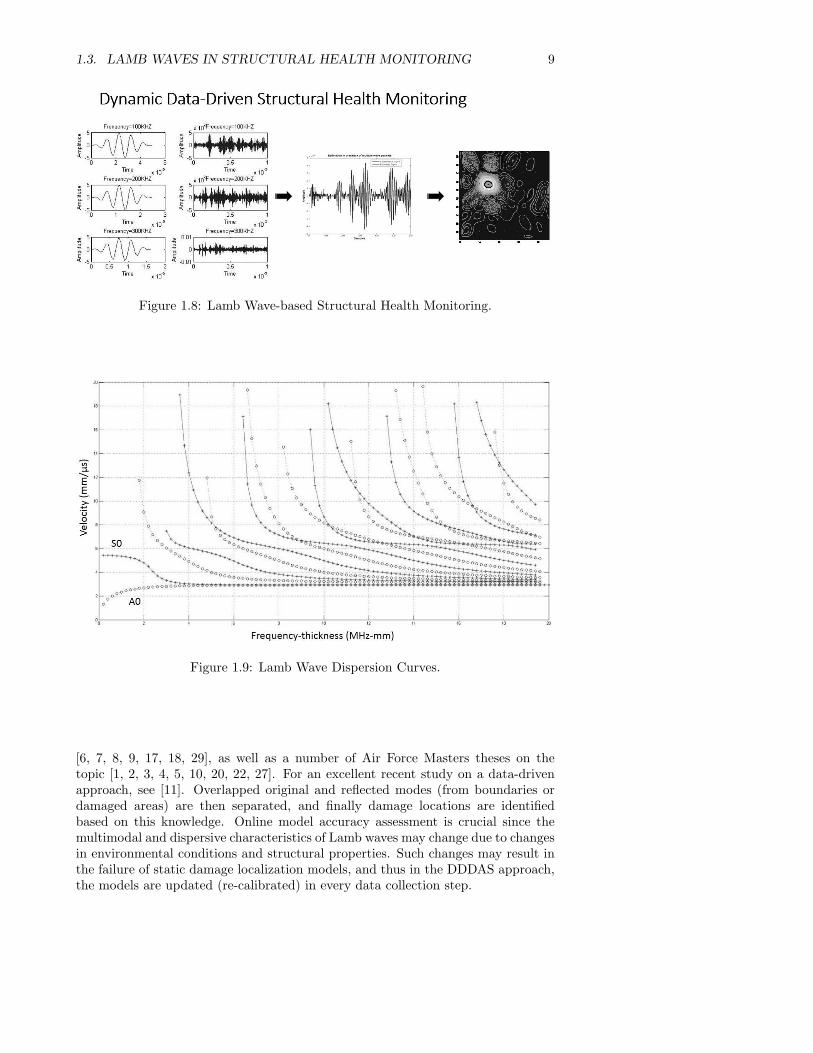
Figure 1.8 lays out the approach to using Lamb waves for SHM. Lamb waves areguided waves that propagate in solid structures. In active SHM systems, Lambwaves may be induced in the structure by ultrasound transducers that may act asactuators and sensors as needed. The propagation takes place in multiple modes.The velocity of each mode at any location of the structure depends on the productof the frequency of excitation and the thickness of the structure at that location.Figure 1.9 displays the phase velocity of different Lamb wave modes in an Aluminumplate. Because of the frequency dependent velocity profiles, the propagation of thesemodes is dispersive. For a detailed introduction to ultrasound waves, see [23]; therehas also been a lot of work in the application of these techniques in SHM (see

1.3. LAMB WAVES IN STRUCTURAL HEALTH MONITORING 9

Figure 1.8: Lamb Wave-based Structural Health Monitoring.

Figure 1.9: Lamb Wave Dispersion Curves.

[6, 7, 8, 9, 17, 18, 29], as well as a number of Air Force Masters theses on thetopic [1, 2, 3, 4, 5, 10, 20, 22, 27]. For an excellent recent study on a data-drivenapproach, see [11]. Overlapped original and reflected modes (from boundaries ordamaged areas) are then separated, and finally damage locations are identifiedbased on this knowledge. Online model accuracy assessment is crucial since themultimodal and dispersive characteristics of Lamb waves may change due to changesin environmental conditions and structural properties. Such changes may result inthe failure of static damage localization models, and thus in the DDDAS approach,the models are updated (re-calibrated) in every data collection step.

10 CHAPTER 1. BAYESIAN METHODS FOR AIRCRAFT SHM

1.3.1 Modeling Lamb Wave Propagation

The dispersive multi-modal propagation of the excitation signal x(t) from an actu-ator to a sensor may be modeled as

y(t) =

M∑

m=1

∫ ∞

−∞

hm(τ)x(t− τ)dτ

where we have assumed that the propagation is linear, hm(t) represent the dispersionand attenuation characteristics of the structure for the mth mode of propagation.Equivalently, we can express the above in the frequency domain as

Y (ω) =

M∑

m=1

Hm(ω)X(ω)

where Y (ω), Hm(ω) and X(ω) are the Fourier transforms of y(t), hm(t) and x(t),respectively. The magnitude response |Hm(ω)| represents the frequency-dependentattenuation characteristics of the structure. This quantity varies with modes as wellas the frequency of excitation. As one would expect, the path length also affectsthe attenuation of the signals in the structure. The phase response depends on thefrequency of excitation through the dispersion curves and the path length. In whatfollows we describe how a model for the dispersion curves can be built.

The governing partial differential equation for displacement in an isotropic platewith density ρ, displacement vector u, and Lame constants µ and λ assuming nobody forces is expressed in vector notation as:

ρu = µ▽2 u+ (λ+ µ)▽ (▽ · u)

where u is the acceleration of displacement. The governing longitudinal wave is:

δ2ϕ

δx2+δ2ϕ

δy2=

1

C2L

δ2ϕ

δt2(1.1)

and the governing shear wave is:

δ2ψ

δx2+δ2ψ

δy2=

1

C2T

δ2ψ

δt2(1.2)

where CL and CT are the longitudinal and transverse wave speeds, respectively.Assuming solutions to the governing equations to be of the form:

ϕ = Φ(y)expi(kx−wt)

ψ = Ψ(y)expi(kx−wt)

we can substitute the above expressions into the governing wave equations (Eqns 1.1–1.2) to get:

Φ(y) = A1 sin(py) +A2 cos(py)

Ψ(y) = B1 sin(qy) +B2 cos(qy)

where A and B are found from the boundary conditions, and:

p2 =w2

C2L

− k2 q2 =w2

C2T

− k2

1.3. LAMB WAVES IN STRUCTURAL HEALTH MONITORING 11

Further development [23] allows us to obtain the Rayleigh-Lamb frequency equa-tions:

us(f, d) ≡tan(qh)

tan(ph)=

−4k2pq

(q2 − k2)2(1.3)

ua(f, d) ≡tan(qh)

tan(ph)=

(q2 − k2)2

−4k2pq(1.4)

We can solve the above two equations numerically to obtain the dispersioncurves. The dispersion curve can then be used along with the length of the pathto estimate the phase response associated with the propagation of each mode. Themagnitude response is typically estimated from the data. Once these quantities areknown, we can use Eqns ( 1.1– 1.2) to estimate the sensor signals. Since each modehas now been characterized we can also use this model to separately identify thedifferent modes and reflections in the sensor signal as shown in the third panel inFigure 1.8. Thus, given an input signal, we use the Fourier transform to obtain thefrequencies involved; these are then propagated according to the dispersion values,and the received signal can be determined. The analytical model for the sensorsignal is then given by:

y(t) = F−1[N∑

m=1

X(ω)Hm(ω)]

where x(t) is the input signal, y(t) is the output signal, m is the mode number,X(ω) the FFT of the input signal, and Hm(ω) the phase response (obtained fromthe dispersion curves). Figure 1.10 shows our mobile robot taking data on the alu-minum plate used for initial studies, as well as some readings from the sensors. Thealuminum panel was 1.6 mm thick, the sensors were VS900-RIC Vallen transducers,and the excitation signal was a 200 KHz 5 cycle, Hann-windowed waveform.

1.3.2 SLAMBOT: Simultaneous Localization and Mapping

using Lamb Waves

We are currently developing a mobile robot platform which can move around on astructure to take data (see Figure 1.10). Based on a modified Systronix Trackbotmobile platform, the SLAMBOT has two attached actuation systems which causethe robot to be lifted off the surface when the ultrasound sensors are used, thus,reducing the interference from the robot on the sensor signals. Our current workis on Simultaneous Localization and Mapping (SLAM) using Lamb waves (see [26]for a detailed account of the SLAM methodology). The damage (and boundary)locations are considered point landmarks since the reflected signal returned from theclosest reflecting point determines the range value. The range calculation methoddescribed earlier (shown in principle in Figure 1.7) is used by finding the arrivaltime of the second Lamb wave signal received (the first being from the straight linepath from the transducer). The total number of features is controlled by the dataacquisition process, and both the range data and the robot motion are assumed tohave been corrupted by additive Gaussian noise.

Because we only use positive landmark detection (landmarks that show up in therange data as opposed to those occluded by other objects), as well as the conditionsgiven above, EKF SLAM works in this setting (see [26]). We therefore estimatethe robot pose st = (x, y, θ) as well as the landmark locations (Fi = fi,xfi,yfi,s)

12 CHAPTER 1. BAYESIAN METHODS FOR AIRCRAFT SHM

Figure 1.10: SLAMBOT for Dynamic Data Acquisition. The SLAMBOT is shownon the left; on the right, the structure is excited in three different locations, and thefinal column is the received signal for each; note that the reflected damage signalcan be seen trailing the direct signal.

i = 1 . . . n, simultaneously using a combined state vector. Then given a motionmode for the robot:

p(st | ut, st−1)

where ut here indicates the robot control. The measurement model is:

p(zt | st, F, nt)

The SLAM problem is to find all landmark locations and the robot’s pose using themeasurements and control values; that is, the posterior:

p(st, F | zt, ut)

We assume feature correspondence is known, and use Algorithm EKF SLAM knowncorrespondences (see Table 10.1 [26], p. 314). The results of a simulation of theLamb wave based range finder are shown in Figure 1.11 (left). In this example,a 2 m X 2 m aluminum plate is used with the origin at the center (thus range inx = [−1, 1] and range in y = [−1, 1]) with one damage location at (−0.4,−0.4). Therobot places the actuator and receiver at six different locations around the damage,and each range value constrains the location of the reflecting point to be on an ellipsewith the actuator and receiver locations as foci. Thus, by using an accumulatorarray and adding a ’vote’ to each location on the ellipse, these six sensed rangevalues allow the determination of the most likely location of the reflecting point(damage in this case). This ’voting’ is done with a Guassian spread which leads tothe smooth accumulator surface shown in the figure. Figure 1.11 (right) shows a2-D visualization of the strength of damage location likelihood based on this data.

1.4. CONCLUSIONS AND FUTURE WORK 13

Figure 1.11: Damage Localization using the Lamb Wave Range Sensor. On theleft is a surface plot view of the accumulator values; on the right a 2-D imagerepresentation.

1.4 Conclusions and Future Work

We propose a Bayesian Computational Sensor Network approach as a formal basisfor Dynamic Data Drive Application Systems. To date, we have shown that thiscan be effective in the 1D domain of heat flow, and we are currently working todevelop a robust aircraft structural health monitoring framework based on the useof Lamb waves. A dynamic data acquisition method using a mobile robot has beendescribed. Future work includes the experimental validation of the approach as wellas a formal analysis of the uncertainty quantification. We are constructing severalmobile robots and will perform experiments using single and multiple robots to mapdamage in plate structures. The experiments will first be performed with Aluminumplates, and then on composite structures.

The field of uncertainty quantification aims to find methods to provide boundson the confidence of inferences about the behavior of physical systems based oncomputational models and sensor data. In order to estimate the error, one canresort to Monte Carlo sampling, or construct a response surface from sampling thesystem. We follow the procedure of Li and Xiu [19, 28] wherein a surrogate model isdeveloped using polynomial chaos: “stochastic solutions are expressed as orthogonalpolynomials of the input random parameters.” We follow the method described inSection 5.2 in [28].

The equations for symmetric (Equation 1.3) and anti-symmetric waves (Equa-tion 1.4) form the basis of our damage analysis range sensor. That is, damage mod-ifies the received signal according to the distance from the actuator to the damageand then on to the receiver. Taking a polynomial chaos approach, the generalizedpolynomial chaos (gPC) approximation to the solution is obtained by projecting u(the function of interest – in this case, the wave speed) onto a polynomial basis, Pi:

u|Pn=

∑

αiPi

14 CHAPTER 1. BAYESIAN METHODS FOR AIRCRAFT SHM

1 1.5 2 2.5 3 3.5 4 4.5 5 5.5 610

−6

10−5

10−4

10−3

10−2

10−1

100

101

Maximum degree of polynomials (N)

Err

or

Semilogy error plot

2 norm errorinfinte norm error

Figure 1.12: First Results in Polynomial Chaos Applied to Lamb Wave Mode Ve-locities.

where the Fourier coefficients are defined as:

αi ≈

∫

uPiρdX =< u,Pi >

where < u,w > is the inner product of v and w. That is, the coefficients of thepolynomial projection are approximated by the inner product of the function u andthe polynomial basis functions.

Figure 1.12 shows a plot of the error generated by sampling the function fun(F,D)(wave speed) exactly and the approximated polynomial up to maximum total degree6. In this case, we are considering the speed of the antisymmetric modes:

fun(F,D) = cpanti

We are currently working on characterizing the uncertainty properties of the rangesensor function described earlier.

Bibliography

[1] A.P. Albert, E. Antoniou, S.D. Leggiero, K.A. Tooman, and R.L. Veglio. ASystems Engineering Approach to Integrated Structural Health Monitoring forAging Aircraft. Master’s thesis, Air Force Institute of Technology, Ohio, March2006.

[2] J.P. Andrews. Lamb Wave Propagation in Varying Thermal Environments.Master’s thesis, Air Force Institute of Technology, Ohio, March 2007.

[3] M. Barker, J. Schroeder, and F. Gurbuz. Assessing Structural Health Monitor-ing Alternatives using a Value-Focused Thinking Model. Master’s thesis, AirForce Institute of Technology, Ohio, March 2009.

[4] M.S. Bond, J. A Rodriguez, and H.T. Nguyen. A Systems Engineering Processfor an Integrated Structural Health Monitoring System. Master’s thesis, AirForce Institute of Technology, Ohio, March 2007.

[5] J.S. Crider. Damage Detection using Lamb Waves for Sructural Health Moni-toring. Master’s thesis, Air Force Institute of Technology, Ohio, March 2007.

[6] Q.-T. Deng and Z.-C. Yang. Scattering of S0 Lamb Mode in Plate with MultipleDamage. Journal of Applied Mathematical Modeling, 35:550–562, 2011.

[7] V. Giurgiutiu. Tuned Lamb Wave Excitation and Detection with PiezoelectricWafer Active Sensors for Structural Health Monitoring. Journal of IntelligentMaterial Systems and Structures, 16(4):291–305, April 2005.

[8] S. Ha and F.-K. Chang. Optimizing a Spectral Element for Modeling PZT-induced Lamb Wave Propagation in Thin Plates. Smart Mater. Struct.,19(1):1–11, 2010.

[9] S. Ha, A. Mittal, K. Lonkar, and F.-K. Chang. Adhesive Layer Effects onTemperature-sensitive Lamb Waves Induced by Surface Mounted PZT Ac-tuators. In Proceedings of 7th International Workshop on Structural HealthMonitoring, pages 2221–2233, Stanford, CA, September 2009.

[10] S.J. Han. Finite Element Analysis of Lamb Waves acting within a Thin Alu-minum Plate. Master’s thesis, Air Force Institute of Technology, Ohio, Septem-ber 2007.

[11] J.B. Harley and J.M.F. Moura. Sparse Recovery of the Multimodal and Disper-sive Characteristics of Lamb Waves. Journal of Acoustic Society of America,133(5):2732–2745, May 2013.

15

16 Computational Sensor Networks

[12] T.C. Henderson. Computational Sensor Networks. Springer-Verlag, Berlin,Germany, 2009.

[13] T.C. Henderson, C. Sikorski, E. Grant, and K. Luthy. Computational SensorNetworks. In Proceedings of the 2007 IEEE/RSJ International Conference onIntelligent Robots and Systems (IROS 2007), San Diego, USA, 2007.

[14] Thomas C. Henderson and Narong Boonsirisumpun. Issues Related to Param-eter Estimation in Model Accuracy Assessment. In Proceedings of the ICCSWorkshop on Dynamic Data Driven Analysis Systems, Barcelona, Spain, June2013.

[15] Thomas C. Henderson, Kyle Luthy, and Edward Grant. Reaction-DiffusionComputation in Wireless Sensor Networks. In Proceedings of the Workshopon Unconventional Approaches to Robotics, Automation and Control Inspiredby Nature, IEEE International Conference on Robotics and Automation, pages13–15, Karlsruhe, Germany, May 2013.

[16] Thomas C. Henderson, Kyle Luthy, and Edward Grant. Reaction-DiffusionComputation in Wireless Sensor Networks. Jounral of Unconventional Com-puting, page to appear, 2014.

[17] B. C. Lee and W. J. Staszewski. Modelling of Lamb Waves for Damage Detec-tion in Metallic Structures: Part I. Wave Propagation. Smart Mater. Struct.,12(5):804–814, October 2003.

[18] B. C. Lee and W. J. Staszewski. Lamb Wave Propagation Modelling for Dam-age Detection: I. Two-dimensional Analysis. Smart Mater. Struct., 16(5):249–259, 2007.

[19] J. Li and D. Xiu. Evaluation of Failure Probability via Surrogate Models.Journal of Computational Physics, 229:8966–8980, 2010.

[20] E. Lindgren, J.C. Aldrin, K. Jata, B. Scholes, and J. Knopp. Ultrasonic PlateWaves for Fatigue Crack Detection in Multi-Layered Metallic Structures. Tech-nical Report AFRL-RX-WP-TP-2008-4044, Air Force Research Laboratory,December 2008.

[21] W.L. Oberkamf and C.J. Roy. Verification and Validation in Scientific Com-puting. Cambridge University Press, Cambridge, UK, 2010.

[22] F. Ospina. An Enhanced Fuselage Ultrasound Inspection Approach for ISHMPurposes. Master’s thesis, Air Force Institute of Technology, Ohio, March 2012.

[23] J. L. Rose. Ultrasound Waves in Solid Media. Cambridge University Press,Cambridge, UK, 1999.

[24] Felix Sawo, Thomas C. Henderson, Christopher Sikorski, and Uwe D.Hanebeck. Sensor Node Localization Methods based on Local Observationsof Distributed Natural Phenomena. In Proceedings of the 2008 IEEE Interna-tional Conference on Multisensor Fusion and Integration for Intelligent Sys-tems (MFI 2006), Seoul, Republic of Korea, August 2008.

[25] Z. Su and L. Ye. Identification of Damage using Lamb Waves. Springer Verlag,Berlin, Germany, 2009.

Index 17

[26] S. Thrun, W. Burgard, and D. Fox. Probabilistic Robotics. MIT Press, Cam-bridge, MA, 2006.

[27] R.T. Underwood. Damage Detection Analysis Using Lamb Waves in RestrictedGeometry for Aerospace Applications. Master’s thesis, Air Force Institute ofTechnology, Ohio, March 2008.

[28] D. Xiu. Fast Numerical Methods for Stochastic Computations: A Review.Communications in Computational Physics, 5(2–4):242–272, 20109.

[29] Y. Ying, Jr. J.H. Garrett, J. Harley, I.J. Oppenheim, J. Shi, and L. Soibelman.Damage Detection in Pipes under Changing Environmental Conditions usingEmbedded Piezoelectric Transducers and Pattern Recognition Techniques. Jnlof Pipeline Systems Engineering and Practice, 4:17–23, 2013.