Bayesian Multi-View Tensor Factorization

Suleiman A Khan1 and Samuel Kaski 1,2

Helsinki Institute for Information Technology HIIT,1 Department of Information and Computer Science, Aalto University, Finland

2 Department of Computer Science, University of Helsinki, Finland{first.last}@aalto.fi

Abstract. We introduce a Bayesian extension of the tensor factoriza-tion problem to multiple coupled tensors. For a single tensor it reducesto standard PARAFAC-type Bayesian factorization, and for two tensorsit is the first Bayesian Tensor Canonical Correlation Analysis method.It can also be seen to solve a tensorial extension of the recent GroupFactor Analysis problem. The method decomposes the set of tensors tofactors shared by subsets of the tensors, and factors private to individ-ual tensors, and does not assume orthogonality. For a single tensor, themethod empirically outperforms existing methods, and we demonstrateits performance on multiple tensor factorization tasks in toxicogenomicsand functional neuroimaging.

1 Introduction

Tensor Factorization methods decompose data into underlying latent factors orcomponents, taking advantage of the natural tensor structure in the data. A widerange of low-dimensional representations of tensors have been proposed earlier[1]. The most well-known models include the CP CANDECOMP/PARAFAC[2,3] and the Tucker 3-mode factor analysis [4]. Tucker is a more generic modelfor complex interactions, whereas CP as an additive combination of rank-1 con-tributions is easier interpretable analogously to matrix factorizations. Recentlywell-regularized probabilistic tensor factorization methods have been introducedfor both CP [5] and Tucker [6], though they are limited to single tensors only.

Two-view tensor models. In order to discover shared patterns between twoco-occuring tensors, joint factorization approaches decompose them into corre-lated factors [7]. Recently, several non-probabilistic methods for Tensor Canon-ical Correlation Analysis have been introduced [8,9,10] extending the matrixcounterparts. The methods impose different constraints but all aim at finding acommon latent representation of two paired tensors.

Two-view matrix models. For paired matrices, integration approacheshave been thoroughly studied. For an overview on nonlinear Canonical Correla-tion Analysis (CCA) see [11] and Bayesian CCA see [12].

Multi-view models. Multi-view modeling integrates information from mul-tiple coupled datasets. For unsupervised multi-view modelling, a method hasrecently been proposed for decomposing several coupled matrices, into compo-nents shared by subsets of the matrices, and components private to each matrix.

2 S.A. Khan and S. Kaski

U

ZX (3)

W(1) W(2) W(3)

X (1) X (2)

Data Tensors View Activation

KComponents

Latent Variables

≈

Fig. 1. Multi-view tensor factorization. Datasets X (1),X (2),X (3) are simultaneouslydecomposed into K components. The Z and U loadings are common to all tensors,while the view-specific loadings W(m) show the intrinsic component-view structure inthe data. The structure is highlighted in W(m) with black representing a componentactive in a view (non-zero loadings), while white is switched off (zero-loadings).

The method was called Group Factor Analysis [13]. As far as we know, methodsfor analysing multiple coupled tensors have not been proposed earlier.

In this paper we formulate and address the novel multi-view tensor factor-ization problem, where the task is to decompose multiple coupled or co-occuringtensors into factors that are shared by subsets of the tensors: one, some or allof them. We formulate a Bayesian model to solve the task, allowing automaticmodel complexity selection and an intrinsic solution for degeneracies. For twoviews, our model is the first Bayesian Tensor Canonical Correlation Analysis.

The rest of the paper is structured as follows: In section 2 we formulatethe novel multi-view tensor factorization problem. In section 3 we present ourBayesian multi-view tensor factorization model and describe its relationship toexisting works. In section 4 we validate the model’s performance in various set-tings and demonstrate its application in a novel toxicogenomics setting and aneuroimaging case. We conclude with discussion in section 5.

Notations: We will denote a tensor as X , a matrix X, vector x and a scalar

x. The Frobenius norm of a tensor is defined as ‖X‖ =√∑

n

∑d

∑l X 2

n,d,l. The

Mode-2 product ×2 between a tensor A ∈ RN×K×L and a matrix B ∈ RD×Kis the projected tensor (A ×2 B) ∈ RN×D×L. A reshaped Khatri Rao product� of two matrices A ∈ RN×K and C ∈ RL×K is the “column-wise matched”outer product of K vector-pairs that results in the tensor (A�C) ∈ RN×K×L.The outer product of two vectors is denoted ◦. The rank of a tensor X is thesmallest number of rank-1 tensors that generate X as their sum. The order ofa tensor is the number of axes in the tensors, also called ways or modes. Fornotational simplicity the model is presented for third order tensors, while it istrivially extendable to higher orders.

2 Multi-View Tensor Factorization

We formulate the novel Multi-view Tensor Factorization (MTF) problem fora collection of m = 1, . . . ,M paired tensors (views), X (1),X (2), . . . ,X (M) ∈RN×Dm×L, as the combined factorization that decomposes the tensors into

Bayesian Multi-View Tensor Factorization 3

factors shared between all, some, or a single tensor. In MTF, each tensor isfactorized into a view-specific matrix of loadings W(m) ∈ RDm×K and a low-dimensional tensor Y ∈ RN×K×L common for all views:

X (m) = Y ×2 W(m) + ε(m) .

Here ε(m) ∈ RN×Dm×L is the noise tensor.The view-specific matrix of loadings W(m) then controls which of the factors

k from the common tensor are active in each view. For convenience we assume afixed number of K factors, with the understanding that for methods capable ofchoosing the number of factors, K is set large enough, and the loadings of extracomponents will automatically become set to zero.

The tensor Y forms the shared latent tensor and can be left unconstrained(equivalent to Tucker1 factorization), or can be further constrained to representany decomposition including Tucker2, Tucker3 or CP. The CP decompositionfactorizes a tensor into a sum of rank-1 tensors, where each rank-1 tensor isthe outer product of vector loadings in all modes, whereas in Tucker variantsthe factor interactions are modelled via a core tensor G. This rank-1 componentdecomposition of CP and its intrinsic axis property from parallel proportionalprofiles [14], along with uniqueness of solutions [15], gives it a very strong in-terpretive power. The Tucker model is more flexible, though, the complex in-teractions via G and non-uniqueness of solutions make its interpretation moredifficult. Therefore, we adapt an underlying CP decomposition for our model.

Figure 1 illustrates MTF for the joint CP-type factorization. More formally,

X (m) =

K∑k=1

Zk ◦Uk ◦W(m)k + ε(m) (1)

= (Z�U)×2 W(m) + ε(m) .

Here Z ∈ RN×K and U ∈ RL×K are the common latent variables and the W(m)

are loadings for each view m.Figure 1 shows the MTF formulation for three tensors, where components

(rows) of W(m) can be active in all, two, or a single view. The loadings W(m)k

are zero for the components k that are not active in view m. A component active

in two or more views has non-zero loadings in the corresponding W(m)k and is

hence shared between them. This specification comprehensively represents theintrinsic structure of the tensor collection.

3 Bayesian Multi-View Tensor Factorization

We formulate a Bayesian treatment of the MTF problem of Equation 1, bycomplementing it with priors for model parameters. Figure 2 summarizes thedependencies between the variables in the decomposition of the M observedtensors X (m) as a graphical model. The main idea is incorporated in plate M ,which represents the view-specific loadings W(m), having two layers of sparsity:

4 S.A. Khan and S. Kaski

τ (m)X (m)

W(m)Z

DMN

U α(m)

β

LM

K

h(m)

Π

Fig. 2. Plate diagram for Bayesian multi-view tensor factorization.

1) view-wise sparsity controlled by h(m) and 2) feature-wise sparsity (across theDM features) controlled by α(m). The view-wise sparsity acts as an on/off switchand allows the model to automatically learn which views share each factor, andalso the total number of factors in the data. The plate K represents probabilisticCP decomposition for each view, where Z and U are the latent variables.

The distributional assumptions of our model (explained in detail below) are:

X (m)n,l ∼ N ((Zn �Ul)×2 W

(m), I(τ (m))−1)

Z ∼ N (0, I)

Ul,k ∼ N (0, (βl,k)−1)

W(m)d,k ∼ h

(m)k N (0, (α

(m)d,k )−1) + (1− h

(m)k )δ0

h(m)k ∼ Bernoulli(πk)

πk ∼ Beta(aπ, bπ)

βl,k ∼ Gamma(aβ , bβ)

α(m)d,k ∼ Gamma(aα, bα)

τ (m) ∼ Gamma(aτ , bτ )

where Gamma(a, b) is parameterized by shape a, rate b.The coupled N×L samples in each tensor X (m) are modelled via the product

of loadings, with a view-specific observation precision τ (m). For the latent vari-ables, we assume a priori independence, and induce an element-wise automaticrelevance determination ARD prior [16] on Ul,k to encourage sparsity.

To infer the interactions between views and components, we make the modelview-wise sparse via a Spike and Slab prior [17] on the projection weights W(m).The spike and slab prior has two parts, one being a delta δ0 function centered atzero and the other some continuous distribution (usually Gaussian). We replacethe Gaussian with an element-wise ARD prior to additionally allow feature-level

Bayesian Multi-View Tensor Factorization 5

sparsity in our model. The ARD is a Normal-Gamma prior that specifies the

precision α(m)d,k controling the scale of each variable. Our element-wise d, k,m

formulation of ARD encourages the loadings within a component-view pair to

be sparse. In the spike and slab construct, the binary value h(m)k drawn from

a Bernoulli distribution gives the component-view activation. If h(m)k = 1, the

component k is active in view m and the loadings W(m)k are sampled from a

corresponding element-wise ARD prior, whereas if h(m)k = 0, the component-

view pair is not active and the loadings W(m)k are set to zero via δ0, inducing

view-wise sparsity.Learning the h(m) activities allows automatic determination of the number

and sharing of factors between the views. This is because if K is set to be large

enough, the model will switch off h(m)k , for all the extra k,m pairs. This yields

the underlying sharing pattern of the views, even producing empty componentsthat are not active in any view. The presense of empty components indicates thatK was set to a large enough value, and the amount of non-empty componentsgives the rank of the view collection. In the construct, πk represents probabilityof activation of each component.

The joint probability of data and parameters can be factorized as follows,and inference is performed via Gibbs sampling:

p(X (1),X (2), ...,X (M), Θ) =

M∏m=1

N∏n=1

L∏l=1

p(X (m)n,l |Zn,Ul,W

(m), τ (m))

p(τ (m))p(Zn)

K∏k=1

p(Ul,k|βl,k)p(βl,k)

D(m)∏d=1

p(W(m)d,k |α

(m)d,k ,h

(m)k )p(α

(m)k ).p(h

(m)k |πk)p(πk)

Degeneracies can complicate the practical use of CP when analyzing real data[18]. Most degeneracies occur due to non-trilinear structure in the data and areidentified by strong negative correlations between two components. To overcomethe problem, researchers have proposed adding orthogonality and non-negativityconstraints that address it by hindering correlations [18,19], but may also effectthe model’s ability to discover PARAFAC’s intrinsic axes.

In our Bayesian formulation, we impose an element-wise ARD prior on thecomponent loadings W(m),U. The element-wise prior regularizes the solution al-lowing determination of precise factor loadings, and is a construct less strict thanorthogonality. Our model should therefore be able to handle weak degeneracies,via a flexible composition that still allows identifying PARAFAC’s intrinsic axes.

3.1 Special Cases and Related Problems

We next present special cases of our model and relate them to the existing works.

6 S.A. Khan and S. Kaski

Sparse Bayesian CP. For m = 1 (a single view) our model reduces to sparseBayesian CP factorization, which can automatically infer the number of compo-nents. In this special case our formulation goes very close to the Bayesian CP[20], the main differences being that they use MAP estimation and do not havefeature-level sparsity.

Other Bayesian versions of CP include a variant specialized for temporaldatasets [5], the fully conjugate model [21], and an exponential family framework[22]. For Tucker factorizations, Chu and Ghahramani [6] formulated Tucker ina probabilistic framework (pTucker) while [23] presented a non-linear variantusing Gaussian processes. All of these follow different assumptions; however,unlike our method, none of them automatically learns the rank of the tensors.Instead, repetitive methods of rank identification are used, though they poseserious scalablity issues for large tensors [1].

Bayesian Tensor CCA. For m = 2, our model is the first Bayesian TensorCCA. The model is related to tensor-CCAs in the classical domain, specificallyto [8,10]. An additional technical difference, besides our Bayesian treatment, isthat the earlier works assume the two tensors to be paired in a single mode(N), while we assume pairing in both N and L. Both settings are sensible andapplicability depends on the nature of the data.

There have also been fusion studies on coupled matrix-tensor factorization,where values in a tensor were predicted with side information from a matrix, orvice versa. A gradient-based least squares optimization approach was presentedin [24], while [25,26] used generalized linear models in a coupled matrix-tensorfactorization framework to solve link prediction and audio processing tasks.

In the matrix domain, a related multi-view problem was recently studied un-der the name of Group Factor Analysis [13]. The goal there was to perform a jointfactor analysis of multiple matrices to find relationships between datasets. Theirmethod also finds components shared between subsets of views but, naturally,works only for matrices.

4 Experiments

We have applied our model on both simulated and real datasets. We will firstdemonstrate in a simulated example the model’s ability to correctly separateshared and view-specific components, as well as precisely identify the factor modeloadings. We next compare our model to the existing state-of-the-art methodson benchmark single-view datasets, to validate that in the single-view specialcase our algorithms are comparable. We then validate our model’s performanceon simulated multi-view tensors and compare to the single-view tensor methodsand the multi-view matrix methods as the existing baselines, ascertaining theadvantage gained by the multi-view tensor decomposition. Finally, we apply ourmethod on multi-view real data tensors on a new problem from toxicogenomicsand a functional neuroimaging dataset, demonstrating the interpretative powerand diverse applicability of the model.

Bayesian Multi-View Tensor Factorization 7

123

True Components

20L

U

30N

Z

40D(1)

W(1)

50D(2)

W(2)

●lo

adin

gs

Estimated Components1234

20L

30N

40D(1)

50D(2)

Tensor A Tensor B1234

Fig. 3. Demonstration of BMTF decomposing two tensors A and B simultaneously,finding the one shared and two view-specific components. Left: Loadings are drawnfor the three components (1 shared, 2 specific) embedded in the data. Right-Bottom:

component-view activation h(m)k for a K = 4 BMTF run. Right: Loadings of the four

BMTF components reveal the shared and specific components.

Our model detects the number and type of components automatically, aslong as it is run with a large enough K, resulting in the extra components get-ting zero loadings. The practical procedure we followed is to increase K untilempty components are found. The experiments were run with the hyperparam-eters aπ, bπ, aα, bα, aβ , bβ , aτ , bτ initialized to 1. To account for high noise in realdatasets, the noise hyperparameters aτ , bτ were initialized assuming a signal-to-noise ratio of 1. All remaining model parameters were learned using Gibbssampling while discarding the first 10,000 samples as the burn-in and using thenext 10,000 samples for estimating the posterior. Our R implementation of themodel is available at http://research.ics.aalto.fi/mi/software/bmtf/.

4.1 Simulated Illustration

We first demonstrate the ability of our BMTF to decompose the data into factorsin a two-view setting. For this purpose two tensor datasets A and B were createdusing three underlying components, one of which is shared between both tensors,while one is specific to each. Figure 3-left shows the 3-mode loadings used tocreate the two tensors, where Z and U are the common 1st and 2nd mode

8 S.A. Khan and S. Kaski

loadings between both tensors while W(1) and W(2) are the 3rd mode loadingsfor tensor A and tensor B, respectively. The shared component (blue) has non-zero loadings in both W(1) and W(2) while the specific ones have non-zero W(m)

loadings in only the corresponding view.BMTF was run with K = 4, i.e., larger than the number of embedded compo-

nents (=3). Figure 3-bottom-right plots the learned h(m)k values for the M = 2

views and K = 4 components. The plot shows that one component is activein both views (black) while one component active in each view, demonstrat-ing that the model correctly separates the shared and view-specific effects. Thefourth component was rightly detected as not active in any of the views, as thedata come from only three components, indicating that the model identifies thecorrect number of components by switching off the extra ones. The discoveredloadings for the 4 components are plotted in Figure 3-right. The plots show thatthe loadings are identified correctly in this simulated example.

4.2 Single View

As discussed in Section 3.1, our method also solves the CP problem as a specialcase when run on a single dataset. We compare our formulation to the existingstate-of-the-art single-view methods on benchmark datasets to validate that ourperformance is at least comparable. These single-view methods have not beengeneralized to multi-view tensors where our main contribution lies.Comparison Methods. We compare to the following state-of-the-art approaches.

ARDCP: Mørup et. al. [20] formulated CP in a Bayesian framework and au-tomatically learn the number of components, using MAP estimation. In compar-ison to them, our model is fully Bayesian and additionally element-wise sparse.

pTucker: Chu and Ghahramani [6] presented a probabilistic version of theTucker model. Tucker is more flexible than CP, though not easy to interpret.

CP: We also compare to the most widely used and updated classical CP im-plementation from the N-way Toolbox (v3.31 of July 2013, http://www.models.life.ku.dk/nwaytoolbox). The implementation solves the factorization usingthe well established Alternating Least Squares ALS algorithm [27]. On the com-putational side, per-iteration complexity of BMTF exceeds ARDCP and CP onlydue to computing K ×K covariance matrices, which is small compared to therest of the computation. Tucker is costlier than CP as it needs to solve for thecore tensor as well, while pTucker reduces its costs with custom solutions.Datasets. We use the three commonly used benchmark datasets in tensor mod-eling from http://www.models.life.ku.dk/nwaydata, namely Amino Acids,Flow Injection Analysis, and Kojima Girls datasets.

We test our model for both its ability to find the number of components andto model the data correctly in a missing value setting. We randomly selectedhalf of the values in the datasets for training the models and predicted theremaining half. The split was repeated independently 100 times. BMTF andARDCP learned the number of components for each split. CP and pTucker wererun with the number of components estimated from the full data using the de-facto standard pftest from N-way toolbox [27].

Bayesian Multi-View Tensor Factorization 9

Table 1. Detection of number of factors, and ability to find the intrinsic structure.The table lists the number of factors of the three real datasets determined by pftest(on full data) from N-way Toolbox and compares the ability of BMTF with other stateof the art methods in a) learning the number of factors and b) prediction error, whendata contains missing values.

Data set Amino Acid Flow Injection Kojima Girls

Size 5 x 201 x 61 12 x 50 x 45 4 x 153 x 20Factors

pftest 3 4 2BMTF 3.0 ± 0.0 4.5 ± 0.5 2.0 ± 0.1ARDCP 3.1 ± 0.3 4.0 ± 0.0 1.2 ± 0.4

Prediction RMSEBMTF 0.0257±0.0003 0.045±0.010 0.189±0.025ARDCP 0.0278±0.0035 0.065±0.001 0.305±0.051CP 0.0256±0.0003 0.053±0.001 1.643±4.098pTucker 0.0250±0.0003 0.049±0.001 0.236±0.055

Results are presented in Table 1. Both BMTF and ARDCP recovered the num-ber of components well despite 50% missing values, with the mean being closeto the number obtained by pftest on full data. The result clearly shows thatautomatic component selection works even in the presence of missing values.

Prediction RMSE results for the first two datasets Amino Acids and FlowInjection show that all methods perform almost comparably and none goes ex-ceedingly wrong, confirming that our method compares well with state-of-the-artsingle-view methods. The third dataset Kojima Girls shows a major differencein the performance of the methods. This dataset is known to have a degeneracyproblem, and hence the standard CP fails to model the data correctly. ARDCPseems to perform better in comparison to CP, and close examination reveals thatthis is because ARDCP tends to skip the degenerate component as can be seenfrom the mean component number of 1.2. Using fewer components is one way ofavoiding the effect of degeneracies. Our method does both, finding the correctnumber of components and being able to cope with degeneracies as is shown bythe best performance. With its flexible parametrization the Tucker is also ableto correctly model non-trilinear structure in the data, which is a characteristicof degeneracies [28]; hence does not suffers from the degeneracy problem.

4.3 Multi-View

To validate the performance of our model in multi-view settings, we applied it tosimulated data sets that have all types of factors, i.e., factors specific to just oneview, factors shared between a small subset of views and factors shared betweenmost of the views. We show that the model can correctly discover the structureas the number of views is increased, while the baseline approaches are unable tofind the correct result.

10 S.A. Khan and S. Kaski

5 10 15

0.0

0.1

0.2

0.3

0.4

0.5

Views

MS

E (

rela

tive)

●

●

●

●

●

●

●

●

●

●

●

●

● ● ●● ● ●

●

BMTFARDCPpTuckerCPGFA

CCSVL

Fig. 4. Performance of Bayesian multi-view tensor factorization compared to single-view tensor methods and multi-view matrix methods (baselines). The number of viewsincreases on the x-axis while the relative mean square error of recovering the underlyingdata is plotted on the y-axis. The single-view methods were tested in two settings a) CCmarked with dashed-lines, where all the tensors are concatenated; b) SVL as dotted-lines, where models are learned for each tensor seperately.

We simulated a data set consisting of M = 16 views with dimensions N =20, L = 5 and Dm randomly sampled between 10 and 100, using a manuallyconstructed set of K=31 factors of the various types. For each component, the

loadings Z:,k, U:,k and W(m):,k were randomly sampled from the standard normal

distribution for all active m. For the non-active views m in the component k,

the W(m):,k were set to zero. The views were then created as:

X (m)=

∑k

Z:,k ◦U:,k ◦W(m):,k

X (m) = X (m)+ ε(m)

where X (m)is the true underlying data while ε(m) is a noise tensor sampled from

a normal distribution with mean zero and variance equivalent to that of X (m).

We ran BMTF for M = 1, . . . , 16. The single-view tensor methods were runin two settings, a) on a concatenation of all views [CC], b) single view learning[SVL], where a model is learned for each view seperatly. BMTF found the correctnumber of components in all cases while ARDCP[CC] failed to detect the correctnumber for M ≥ 4. The other two methods, CP and pTucker, were run with thetrue number of factors. In single view learning [SVL], the methods were unableto identify the sharing between components, as they do not solve the multi-view

Bayesian Multi-View Tensor Factorization 11

Tensor ViewsGene Expression Toxicity

5

15

25

Com

pone

nts

Fig. 5. Component activations in the toxicogenomics dataset indicate 3 shared compo-nents between the disease-specific gene expression responses and toxicity measurementsof the drugs. The presence of several empty components indicates that K = 30 wasenough to model the data.

problem addressed by BMTF. For completeness, we also compare our method tomulti-view matrix FA (GFA) [13] by matricizing the tensors X (M) ∈ RN×Dm×L

into matrices X(M) ∈ R(N×L)×Dm .We measured the models’ performance in terms of the recovery error of the

missing data. Defining X̂ (m) as the model’s estimate of the data, the recoveryerror is computed as the relative mean square error ‖X̂ (m) − X (m)‖2/‖X (m) − X (m)‖2

averaged over all the views.Figure 4 plots the recovery error of our method as a function of the number

of views. Our model’s performance is stable as the number of views increases andoutperforms all the baseline tensor and matrix alternatives. Single-view methods,applied to a data set which contains all tensors concatenated, deteriorate rapidly;while by learning each tensor seperately they are unable to discover the sharedpattern. The matricized method (GFA) performs comparably to the single-viewtensor methods. The experiment confirms that the specific multi-view tensorproblem cannot be optimally solved with methods not designed for the purpose,and that our method fulfills its promise.

4.4 Application Scenarios and Interpretation

We next demonstrate the method at work on multi-view tensor datasets in po-tential use cases of BMTF. The first application represents a new problem atthe juncture of toxicity and bioinformatics, while the second is a functional neu-roimaging case.Toxicogenomics. We analyzed a novel drug toxicity response problem, wherethe tensors arise naturally when gene expression responses of multiple drugs aremeasured for multiple diseases (different cancers) across the genes. The datacontain two views, the measurement of post-treatment gene expression, and sen-sitivity of the cells to the drug. The key question that BMTF can answer is,which parts of the responses are specific to individual types of cancer and whichoccur across cancers, and which of them are related to drugs effectiveness. Thesepatterns, if uncovered, can help understand the mechanisms of toxicity [29].

12 S.A. Khan and S. Kaski

−2 0 2−3 0 3

BLOOD U: 1.00

CY

P1B

1C

CN

E2

KLF

10H

SPA

1BH

SPA

6H

SPA

1AB

AG

2R

BM

23B

AG

3D

NA

JB4

DN

AJB

1H

SP

H1

HS

PA4L

SE

RP

INH

1P

4HA

2

BREAST U: 0.94

PROSTATE U: 0.79

W:−

1.05

W:−

1.26

W:−

1.10

W: 2

.93

W: 2

.44

W: 1

.40

W: 1

.19

W: 1

.15

W: 1

.14

W: 1

.52

W: 1

.80

W: 1

.73

W: 1

.85

W: 1

.65

W: 1

.57

thioridazinesecurinine

alvespimycintanespimycin

geldanamycin

Z: 0.14Z: 0.46Z: 0.86Z: 0.95Z: 1.00

GI5

0

TG

I

LC50

thioridazinesecurinine

alvespimycintanespimycin

geldanamycin

Z: 0.14Z: 0.46Z: 0.86Z: 0.95Z: 1.00

thioridazinesecurinine

alvespimycintanespimycin

geldanamycin

Z: 0.14Z: 0.46Z: 0.86Z: 0.95Z: 1.00

W: 1

.48

W:−

0.21

W:−

0.77

Fig. 6. Component 1 captures the well-known heatshock protein response. The topgenes (left) and toxicity indicators (right) from the two views are plotted as columns,and the three different cancers as rows. The component links the strong upregulationof the heatshock protein genes (red) to high toxicity (green) in the top three drugs, allof which are heatshock protein inhibitors.

The dataset contained two views. The first, m = 1, contained the post-treatment differential gene expression responses D1 = 1106 of several drugsN = 78 as measured over multiple cancer types L = 3. The second, m = 2,contained the corresponding drug sensitivity measurements D2 = 3. The geneexpression data were obtained from the connectivity map [30] that containedresponse measurements of three different cancers: Blood Cancer, Breast Cancerand Prostate Cancer. The data were processed so that gene expression valuesrepresent up (positive) or down (negative) regulation from the untreated (base)level. Strongly regulated genes were selected, resulting in D1 = 1106. The drugscreen data for the three cancer types were obtained from the NCI-60 database[31], measuring toxic effects of drug treatments via three different criteria: GI50(50% growth inhibition), LC50 (50% lethal concentration) and TGI (total growthinhibition). The data were processed to represent the drug concentration usedin the connectivity map to be positive when toxic, and negative when non-toxic.

BMTF was run with K=30, resulting in 3 components shared between boththe gene expression and toxicity views, revealing that some patterns are indeedshared (Figure 5). These shared components form hypotheses about underlyingbiological processes that characterize toxic responses of the drugs.

Bayesian Multi-View Tensor Factorization 13

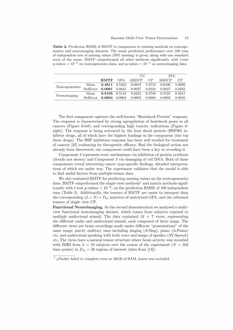
Table 2. Prediction RMSE of BMTF in comparison to existing methods on toxicoge-nomics and neuroimaging datasets. The mean prediction performance over 100 runsof independent sets of missing values (50% missing) is given, along with one standarderror of the mean. BMTF outperformed all other methods significantly with t-testp-values < 10−6 on toxicogenomics data, and p-values < 10−4 on neuroimaging data.

CC SVLBMTF GFA ARDCP CP ARDCP CP

ToxicogenomicsMean 0.4811 0.5223 0.8919 5.3713 0.6438 5.0699

StdError 0.0061 0.0041 0.0027 0.0310 0.0047 0.0282

NeuroimagingMean 0.5105 0.5144 0.6224 0.5740 0.5725 0.5611

StdError 0.0004 0.0004 0.0003 0.0004 0.0003 0.0010

The first component captures the well-known “Heatshock Protein” response.The response is characterized by strong upregulation of heatshock genes in allcancers (Figure 6-left) and corresponding high toxicity indications (Figure 6-right). The response is being activated by the heat shock protein (HSP90) in-hibitor drugs, all of which have the highest loadings in the component (the topthree drugs). The HSP inhibition response has been well studied for treatmentof cancers [32] evaluating its therapeutic efficacy. Had the biological action notalready been discovered, our component could have been a key in revealing it.

Component 2 represents toxic mechanisms via inhibition of protein synthesis(details not shown) and Component 3 via damaging of cell DNA. Both of thesecomponents reveal interesting cancer type-specific findings, detailed interpreta-tions of which are under way. The experiment validates that the model is ableto find useful factors from multiple-tensor data.

We also evaluated BMTF for predicting missing values on the toxicogenomicsdata. BMTF outperformed the single-view methods1 and matrix methods signif-icantly with t-test p-values < 10−6, on the prediction RMSE of 100 independentruns (Table 2). Additionally, the tensors of BMTF are easier to interpret thanthe corresponding (L×N)×Dm matrices of matricized GFA, and the reformedtensors of single view CP.

Functional Neuroimaging. As the second demonstration we analysed a multi-view functional neuroimaging dataset, which comes from subjects exposed tomultiple audiovisual stimuli. The data contained M = 7 views, representingthe different audio and audiovisual stimuli, each composed of three songs. Thedifferent views are brain recordings made under different “presentations” of thesame songs: purely auditory ones including singing (A:Sing), piano (A:Piano)etc, and audiovisual speaking with both voice and image of speaker (AV:Speech)etc. The views have a natural tensor structure where brain activity was recordedwith fMRI from L = 10 subjects over the course of the experiment (N = 162time points) in Dm = 32 regions of interest (data from [13]).

1 pTucker failed to complete even on 50GB of RAM, hence was excluded.

14 S.A. Khan and S. Kaski

50

150

250

Com

pone

nts

Tensor Views

A: Sing

A: Pian

o

A: Spe

ech

A: Sing

Piano

AV: Sing

AV: Pian

o

AV: Spe

ech

1

3

Top

Com

pone

nts

Fig. 7. Top: Component activations in the neuroimaging dataset. The componentsshared between subsets of views capture potentially interesting variation, separatedfrom the view-specific “structured noise” or non-interesting variation. Bottom:Zoomed inset of top components based on subject (U) loadings. The first componentis active in both speech views.

BMTF was run with K = 300 and the h(m) profile is shown in Figure 7. Theplot indicates that there exist several potentially interesting components sharedbetween different subsets of views. The large number of view-specific componentsmodel “structured noise”, i.e., mostly brain activity not related to the stimuli.

The goal of the fMRI study was to find responses that generalize acrossthe subjects and describe relationships of the different presentation conditions(views). We selected components generalizing across subjects by sorting thembased on the subject (U) loadings, and explain the first one here to concretizewhat the method can produce. The first component is active in the speech-related views, pure audio (A:Speech), and combined audio-visual (AV:Speech)views, indicating that it captures speech-related activity. A closer look at theW(m) loadings for the views shows activation of the same auditory regions ofthe brain, demonstrating the signal is neuroscientifically relevant.

Quantitatively, BMTF fits the data better than simpler alternatives as demon-strated by the missing value prediction in Table 2, while in comparison to theanalysis of [13], it extracts more components having consistent behaviour overthe subjects, indicating that taking the tensorial nature of data into accountimproves detection of structure.

5 Discussion

We introduced a novel multi-view tensor factorization problem, of collectivelydecomposing multiple paired tensors into factors. We factorize the tensors into

Bayesian Multi-View Tensor Factorization 15

PARAFAC-type (equivalently, CP-type) components, each shared by a subsetof the tensors, from one to all. We introduced a Bayesian multi-view tensorfactorization (BMTF) model that solves the problem via a joint CP-type de-composition of tensors while learning the precise type and number of factorsautomatically. In the special case of two tensors, our method is simultaneouslyalso the first Bayesian tensor canonical correlation analysis (CCA) method. Themodel can also be considered as an extension of the matrix-based Group FactorAnalysis method [13] to tensors.

We validated the model’s performance in identifying components on simu-lated data. The model was then demonstrated on a new toxicogenomics problemand a neuroimaging dataset, yielding interpretable findings with detailed inter-pretations on-going. Initial evidence suggests that taking the tensor nature ofdata into account makes the results more accurate and precise. In particular,the model is able to handle degenerate solutions well, making the formulationapplicable to a wider set of datasets.

Acknowledgments. The work was supported by the Academy of Finland (140057;Finnish Centre of Excellence COIN, 251170) and the FICS doctoral programme.We also acknowledge Aalto Science-IT resources.

References

1. Kolda, T., Bader, B.: Tensor decompositions and applications. SIAM Review51(3) (2009) 455–500

2. Carroll, J.D., Chang, J.J.: Analysis of individual differences in multidimensionalscaling via an n-way generalization of Eckart-Young decomposition. Psychometrika35(3) (1970) 283–319

3. Harshman, R.A.: Foundations of the parafac procedure: models and conditions foran explanatory multimodal factor analysis. UCLA Working Papers in Phonetics16 (1970) 1–84

4. Tucker, L.R.: Some mathematical notes on three-mode factor analysis. Psychome-trika 31(3) (1966) 279–311

5. Xiong, L., Chen, X., Huang, T.K., Schneider, J., Carbonell, J.G.: Temporal collab-orative filtering with bayesian probabilistic tensor factorization. In: Proceedingsof SIAM Data Mining. Volume 10. (2010) 211–222

6. Chu, W., Ghahramani, Z.: Probabilistic models for incomplete multi-dimensionalarrays. In: Proceedings of AISTATS, JMLR W&CP. Volume 5. (2009) 89 – 96

7. Lee, S.H., Choi, S.: Two-dimensional canonical correlation analysis. Signal Pro-cessing Letters, IEEE 14(10) (2007) 735–738

8. Kim, T.K., Cipolla, R.: Canonical correlation analysis of video volume tensors foraction categorization and detection. IEEE Transactions on Pattern Analysis andMachine Intelligence 31(8) (2009) 1415–1428

9. Yan, J., Zheng, W., Zhou, X., Zhao, Z.: Sparse 2-d canonical correlation analysisvia low rank matrix approximation for feature extraction. IEEE Signal ProcessingLetters 19(1) (2012) 51–54

10. Lu, H.: Learning canonical correlations of paired tensor sets via tensor-to-vectorprojection. In: Proceedings of IJCAI. (2013) 1516–1522

16 S.A. Khan and S. Kaski

11. Hardoon, D.R., Szedmak, S., Shawe-Taylor, J.: Canonical correlation analysis: Anoverview with application to learning methods. Neural Computation 16(12) (2004)2639–2664

12. Klami, A., Virtanen, S., Kaski, S.: Bayesian canonical correlation analysis. Journalof Machine Learning Research 14 (2013) 965–1003

13. Virtanen, S., Klami, A., Khan, S.A., Kaski, S.: Bayesian group factor analysis. In:Proceedings of AISTATS, JMLR W&CP 22. (2012) 1269–1277

14. Cattell, R.B.: Parallel proportional profiles and other principles for determiningthe choice of factors by rotation. Psychometrika 9(4) (1944) 267–283

15. Kruskal, J.B.: Three-way arrays: rank and uniqueness of trilinear decompositions,with application to arithmetic complexity and statistics. Linear Algebra and itsApplications 18(2) (1977) 95 – 138

16. Neal, R.M.: Bayesian learning for neural networks. Springer-Verlag (1996)17. Mitchell, T.J., Beauchamp, J.J.: Bayesian variable selection in linear regression.

Journal of the American Statistical Association 83(404) (1988) 1023–103218. Krijnen, W., Dijkstra, T., Stegeman, A.: On the non-existence of optimal solutions

and the occurrence of degeneracy in the candecomp/parafac model. Psychometrika73(3) (2008) 431–439

19. Srensen, M., Lathauwer, L., Comon, P., Icart, S., Deneire, L.: Canonical polyadicdecomposition with a columnwise orthonormal factor matrix. SIAM Journal onMatrix Analysis and Applications 33(4) (2012) 1190–1213

20. Mørup, M., Hansen, L.K.: Automatic relevance determination for multiway models.Journal of Chemometrics 23(7-8) (2009) 352 – 363

21. Hoff, P.D.: Hierarchical multilinear models for multiway data. ComputationalStatistics & Data Analysis 55(1) (2011) 530 – 543

22. Hayashi, K., Takenouchi, T., Shibata, T., Kamiya, Y., Kato, D., Kunieda, K.,Yamada, K., Ikeda, K.: Exponential family tensor factorization: an online extensionand applications. Knowledge and Information Systems 33(1) (2012) 57–88

23. Xu, Z., Yan, F., Qi, A.: Infinite tucker decomposition: Nonparametric bayesianmodels for multiway data analysis. In: Proceedings of ICML. (2012) 1023–1030

24. Acar, E., Rasmussen, M.A., Savorani, F., Naes, T., Bro, R.: Understanding datafusion within the framework of coupled matrix and tensor factorizations. Chemo-metrics and Intelligent Laboratory Systems 129 (2013) 53 – 63

25. Ermis, B., Acar, E., Cemgil, A.T.: Link prediction in heterogeneous data viageneralized coupled tensor factorization. Data Mining and Knowledge Discovery(2013) 1–34

26. Yilmaz, K.Y., Cemgil, A.T., Simsekli, U.: Generalised coupled tensor factorisation.In: Proceedings of NIPS. (2011) 2151–2159

27. Andersson, C.A., Bro, R.: The N-way toolbox for MATLAB. Chemometrics andIntelligent Laboratory Systems 52(1) (2000) 1 – 4

28. Lundy, M.E., Harshman, R.A., Kruskal, J.B.: A two-stage procedure incorporatinggood features of both trilinear and quadrilinear models. Multiway data analysis(1989) 123–130

29. Hartung, T., Vliet, E.V., Jaworska, J., Bonilla, L., Skinner, N., Thomas, R.: Foodfor thought ... systems toxicology. ALTEX 29(2) (2012) 119–128

30. Lamb, J., et al.: The connectivity map: Using gene-expression signatures to connectsmall molecules, genes, and disease. Science 313(5795) (2006) 1929–1935

31. Shoemaker, R.H.: The nci60 human tumour cell line anticancer drug screen. NatureReviews Cancer 6(10) (2006) 813–823

32. Kamal, A., et al.: A high-affinity conformation of HSP90 confers tumour selectivityon HSP90 inhibitors. Nature 425(6956) (2003) 407–410