Supplementary materials for this article are available at 10.1007/s13253-014-0167-0.

Bayesian Methods for Hierarchical DistanceSampling Models

C.S. OEDEKOVEN, S.T. BUCKLAND, M.L. MACKENZIE, R. KING,K.O. EVANS, and L.W. BURGER Jr.

The few distance sampling studies that use Bayesian methods typically consideronly line transect sampling with a half-normal detection function. We present aBayesian approach to analyse distance sampling data applicable to line and point tran-sects, exact and interval distance data and any detection function possibly includingcovariates affecting detection probabilities. We use an integrated likelihood which com-bines the detection and density models. For the latter, densities are related to covariatesin a log-linear mixed effect Poisson model which accommodates correlated counts. Weuse a Metropolis-Hastings algorithm for updating parameters and a reversible jump al-gorithm to include model selection for both the detection function and density models.The approach is applied to a large-scale experimental design study of northern bob-white coveys where the interest was to assess the effect of establishing herbaceousbuffers around agricultural fields in several states in the US on bird densities. Resultswere compared with those from an existing maximum likelihood approach that analysesthe detection and density models in two stages. Both methods revealed an increase ofcovey densities on buffered fields. Our approach gave estimates with higher precisioneven though it does not condition on a known detection function for the density model.

Key Words: Designed experiments; Hazard-rate detection function; Heterogene-ity in detection probabilities; Metropolis–Hastings update; Point transect sampling;RJMCMC.

1. INTRODUCTION

Bayesian methods are becoming increasingly popular for modelling wildlife popula-tions and abundances (e.g. Buckland, Goudie, and Borchers 2000, Marcot et al. 2001;Durban and Elston 2005; Schmidt et al. 2009; King et al. 2010). However, few distance

C.S. Oedekoven (B) is a Research Fellow in Statistics (E-mail: cso2@st-andrews.ac.uk), S.T. Buckland is a Pro-fessor of Statistics, M.L. Mackenzie is Lecturer in Statistics, and R. King is a Reader in Statistics, Centre forResearch into Ecological and Environmental Modelling, School of Mathematics and Statistics, University ofSt Andrews, St Andrews, KY16 9LZ, UK. K.O. Evans is a former Research Associate and L.W. Burger Jr. isa Professor of Wildlife Ecology and Management, Department of Wildlife, Fisheries & Aquaculture, MississippiState University, Box 9690, Mississippi State, MS 39762, USA.

© 2014 International Biometric SocietyJournal of Agricultural, Biological, and Environmental Statistics, Accepted for publicationDOI: 10.1007/s13253-014-0167-0

C.S. OEDEKOVEN ET AL.

sampling studies have taken a Bayesian approach. Karunamuni and Quinn (1995) devel-oped a Bayes estimator for f (0) using a half-normal detection function (and a gammaprior), where f (0) is a quantity estimated from the distance data that allows observedcounts to be adjusted for imperfect detection. The approach makes use of the conjugateproperty between the normal and gamma distributions. Other studies have built upon thisapproach. Eguchi and Gerrodette (2009) extended this model by including a binomial like-lihood for the encounter rate along the line and described a joint posterior distribution forthe density model and effective strip width. Gimenez et al. (2009) implemented an estima-tor for f (0) using BUGS software, while Zhang (2011) developed an empirical Bayes esti-mator for f (0). These studies follow a similar approach in that they present their methodsfor line-transect data and use the half-normal detection function. We describe a Bayesianapproach to density estimation from distance sampling data for both line and point transectdata applicable to any detection function that uses a hierarchical modelling approach.

Hierarchical distance sampling models have also been developed by e.g. Royle and Do-razio (2008, Chapter 7.1). These authors employ a likelihood that combines the detectionfunction and the binomial model using the marginal probability of encounter (estimatedfrom the detection function) and a data augmentation approach for unobserved groups.The data augmentation approach was adopted by Schmidt et al. (2012), who added a groupsize model, and Conn, Laake, and Johnson (2012), who extended the approach for doubleobserver data.

In contrast, we use an integrated likelihood that combines the likelihood components ofthe detection and count models. For the latter, we use a Poisson likelihood for the distancesampling counts that incorporates a component corresponding to the detection function,thus allowing for undetected animals on the surveyed strip (line transects) or circular plot(point transects). In comparison to Eguchi and Gerrodette (2009), who use a binomiallikelihood to scale up from density at the line to density in the study area, our Poissonmodel relates animal counts to covariates via a log-link function. This approach does notrely on random placement of samplers in the study area to the same extent as the design-based approach for the binomial model (Hedley and Buckland 2004). Similar to Chelgrenet al. (2011), we include a random effect for site in the Poisson model to accommodatecorrelated counts due to e.g. repeat counts at the same site. The parameter space is exploredusing a Metropolis–Hastings (MH) updating algorithm so that different prior distributionsfor the parameters are easily implemented, and a reversible jump Markov chain MonteCarlo (RJMCMC) algorithm allows for model uncertainty to be incorporated. This mayinclude different key functions for the detection function model and different covariatecombinations for both the detection function and the count models.

These developments were motivated by a large-scale experimental study to assess the ef-fects of establishing conservation buffers along field margins on density of several speciesof conservation interest such as the northern bobwhite (Colinus virginianus). Pairs of pointswere set up at the edge of fields in farmland in 13 states in the USA. These pairs of pointsconsisted of one point on a buffered treatment field and one on a nearby non-buffered con-trol field and will be referred to as sites in the following. Point transect surveys of coveys(fall–winter stable social units of 10–15 individual birds) were conducted at least once butup to three times per year in autumn from 2006 to 2008.

BAYESIAN METHODS FOR HIERARCHICAL DISTANCE SAMPLING MODELS

In the following we begin by developing the integrated likelihood (Section 2), describethe Bayesian approach (Section 3) and analyse bobwhite covey data using our Bayesianapproach (and a maximum likelihood approach for comparison) (Section 4). Lastly, wecontrast our Bayesian approach with existing studies using distance sampling likelihoods(Section 5).

2. AN INTEGRATED LIKELIHOOD FOR DISTANCE SAMPLINGDATA

To obtain abundance estimates of a population of interest using distance sampling meth-ods, lines or points may be placed in the study area according to some design (see Bucklandet al. 2001, for details). Each line or point is surveyed at least once following the distancesampling protocol where the observer travels along the line (line transects) or remains atthe point for a fixed amount of time (point transects). Detections are recorded along withthe perpendicular distance from the line to the detection or radial distance from the pointto the detection. These distances may be recorded exactly or in predetermined distance in-tervals. Thus, surveys of this type produce two types of data: firstly, the observed distancesye with e = 1,2,3, . . . , n (n being the total number of detections) or observed distancesni in each of i = 1,2,3, . . . , I distance intervals (where

∑Ii=1 ni = n); secondly, the ob-

served number of detections or counts np at line or point p along with the effort data,which at bare minimum consists of the size of the search area. In case detections are madeof single animals, the observed counts at the line (point) are equivalent to the number ofdetections at the line (point). These two types of data, distances and counts, give rise tothe two components of the integrated likelihood described in this section. However, if de-tections are made of groups of animals (rather than single individuals), a third type of datagenerated from a distance sampling survey is cluster size se , which represents the numberof individuals within the eth detected group. For simplicity, we ignore cluster sizes forthis study. Methods could, however, be extended to accommodate group sizes larger thanone. This may be done by considering counts of individuals (rather than detections) in thecount model described below or by including a model for cluster sizes. The latter maybe desirable e.g. if group size data are overdispersed (e.g. Cañadas and Hammond 2006;Schmidt et al. 2012).

In contrast to many existing covariate models for distance sampling data (e.g. Hedleyand Buckland 2004; Buckland et al. 2009), the proposed integrated likelihood deals withboth components of the data simultaneously—similar to e.g. Royle, Dawson, and Bates(2004) and Sillett et al. (2012). It consists of the likelihood components for the detectionfunction, which is denoted by Ly(θ) for exact distance data (see Equation (2.5) below forinterval data), and the Poisson likelihood for observed counts, Ln(β|θ). We use θ and β tosummarise the detection function and Poisson model parameters, respectively. These aredefined in more detail below. The integrated likelihood is the product of the two compo-nents:

Ln,y(β, θ) = Ly(θ)Ln(β|θ) (2.1)

C.S. OEDEKOVEN ET AL.

(modified from Buckland et al. 2004, Chapter 2). We consider each individual likelihood

component in Ln,y(β, θ) and begin with Ly(θ).

2.1. LIKELIHOOD COMPONENT FOR THE DETECTION FUNCTION

Let f (y|θ) denote the probability density function of observed distances which is given

as

f (y|θ) = π(y)g(y|θ)∫ w

0 π(y)g(y|θ) dy, (2.2)

where y is the observed distance from the line (point), and w is the truncation dis-

tance (i.e. the furthest distance from the line (point) included in the analysis, Thomas

et al. 2010). π(y) describes the expected distribution of animals with respect to the line

(π(y) = 1/w) or point (π(y) = 2y/w2). The detection function g(y|θ) may be mod-

elled e.g. as half-normal (g(y|θ) = exp(−y2/2σ 2), with θ = {σ }) or hazard-rate (g(y|θ) =1 − exp(−(y/σ )−τ ), with θ = {σ, τ }). The likelihood component, which is conditional on

the number of detections n, may be expressed as

Ly(θ) =n∏

e=1

f (ye|θ), (2.3)

where ye refers to the eth detection (Buckland et al. 2004).

When detections are recorded in distance intervals, let fi denote the probability that a

detected animal is in the ith interval that is delineated by the cutpoints ci−1 and ci :

fi(θ) =∫ ci

ci−1f (y|θ) dy

∫ w

0 f (y|θ) dy, (2.4)

where the truncation distance, w, corresponds to the outermost cutpoint. Then, the multi-

nomial likelihood LyG replaces Ly in Equation (2.1) and may be expressed as

LyG(θ) =(

n!∏I

i=1 ni !) I∏

i=1

fi(θ)ni , (2.5)

where ni is the number of detected animals in the ith interval.

Note that in Equations (2.3) and (2.5), detections from all sites are pooled in one

detection function. For modelling heterogeneity using multiple covariate distance sam-

pling (MCDS) methods, the scale parameter σ of the half-normal or hazard-rate detec-

tion function is modelled as a function of covariates (σ (z) = δ0 × exp(∑Q

q=1 zqδq), where

δq , q = 0,1,2, . . . ,Q replace σ in θ ) (Marques and Buckland 2003), and the zq represent

the values of the qth covariate.

BAYESIAN METHODS FOR HIERARCHICAL DISTANCE SAMPLING MODELS

2.2. LIKELIHOOD COMPONENT FOR THE COUNT MODEL

For the log-linear Poisson model, Ln(β|θ), we begin by considering a study design that

consists of multiple sites each containing one or more lines (points) that are surveyed at

least once. If all sites contain only one line (point) and surveys are not repeated, each count

may be considered independent under conditions described by Buckland et al. (2001).

However, if sites contain clusters of lines (points) and/or sites were surveyed more than

once, this assumption is violated. We deal with this by grouping counts from the same site

and fitting a random effect coefficient for each site in the following count model (see below

in this section).

Here, we consider counts njpr at visit r to line or point p at site j as a Poisson random

variable with E(njpr) = λjpr . To adjust counts for imperfect detection out to distance w,

f (y|θ) from Equation (2.2) is used to estimate the effective area ν(θ), which is defined

as the area beyond which as many animals are seen as are missed within (Buckland et al.

2001). Thus, the density Djpr may be expressed as

Djpr = λjpr/ν(θ). (2.6)

For line transects, ν(θ) = 2lp∫ w

0 g(y|θ) dy, where lp is the length of the line surveyed; for

point transects, ν(θ) = 2π∫ w

0 yg(y|θ) dy. These definitions for ν are given for the case

where all detections are pooled in a global detection function. When modelling hetero-

geneity, e.g. using MCDS methods, the effective area may vary between lines (points), and

the global ν becomes νjpr .

However, when replacing Djpr with a covariate model (Djpr = exp(β0 + bj +∑K

k=1 xkjprβk)) and rearranging Equation (2.6), we obtain a model for the expected counts

λjpr , which is now a function of the density model parameters β and conditional on detec-

tion function parameters θ :

λjpr(β|θ) = exp

(

β0 + bj +K∑

k=1

xkjprβk + ln(ν(θ)

))

. (2.7)

Here β0 is the intercept, bj the random effect for site j (bj ∼ N(0, σ 2b )), xk the k co-

variates, xkjpr the covariate values measured during visit r to that line or point, and βk the

associated coefficients. The vector β = {β0, β1, β2, . . . , βK,σb} denotes the parameters as-

sociated with the covariates affecting densities and the random effect standard deviation.

Equation (2.7) is given for the general case where lines or points that may produce corre-

lated counts, due to closeness in space and/or due to repeated measurements at the same

line (point), are grouped together as site j. The inclusion of a random effect for site ac-

commodates covariances for these measurements. However, in cases where lines (points)

follow a random survey design (Buckland et al. 2001) and each line (point) is surveyed

only once, the random effect term may be omitted.

C.S. OEDEKOVEN ET AL.

Using this model for λjpr , the likelihood for the count model (Equation (2.7)), condi-tional on detection function parameters θ , may be expressed as

Ln(β|θ) =J∏

j=1

∫ ∞

−∞

( Pj∏

p=1

Rj∏

r=1

(λjpr )njpr exp(−λjpr)

njpr ! × 1√

2πσ 2b

exp

(

− 1

2σ 2b

b2j

))

dbj ,

(2.8)where J refers to the total number of sites, and Pj and Rj refer to the total number oflines (points) at and visits to the j th site, respectively. Ln(β|θ) forms the second likeli-hood component in Equation (2.1). Note that in a maximum likelihood context the like-lihood function including a random effect (for which normality is assumed) is generallyformulated with an integral as shown in Equation (2.8) as the random effect is integratedout analytically (or by approximation) and the individual coefficients bj are not estimated(e.g. McCulloch and Searle 2001). In the Bayesian context, the random effect is not in-tegrated out analytically. Here, we use a data augmentation scheme where the individualcoefficients bj are included as parameters (or auxiliary variables) within the model andupdated within the MCMC algorithm (see below).

3. THE BAYESIAN APPROACH

3.1. HIERARCHICAL MODELS

Using a Bayesian approach, random-effects models can be implemented using hierar-chical models where the standard deviation of the random effect (σb from Equation (2.8))is considered a random variable with a distribution rather than as a fixed value (Davison2003). Individual random effects coefficients (bj from Equations (2.7) and (2.8)) are fittedin the model and updated at each iteration of the chain in a Markov chain Monte Carlo(MCMC) algorithm.

Prior beliefs regarding the parameters, such as knowledge obtained from a previousstudy, may be included in the current study via the prior distribution. This may allow infer-ence on model parameters in cases where too few data exist in the current study to obtainmaximum likelihood estimates with great precision (e.g. Eguchi and Gerrodette 2009).

3.2. MCMC ALGORITHM

An MCMC algorithm is used to explore the posterior distribution of the parametersgiven the data. Commonly used MCMC methods are the Gibbs sampler and Metropolis–Hastings (MH) update. We focus on the MH update (Hastings 1970; Metropolis et al. 1953)as some of the likelihood functions that may be used to form the posterior conditional dis-tributions of parameters are non-standard (e.g. half-normal or hazard-rate detection func-tion that may include a covariate model for the scale parameter). In particular, we usea random walk single-update MH algorithm with normal proposal density. The proposalvariance for each parameter may be obtained via pilot-tuning (Gelman, Roberts, and Gilks1996). See Appendix A.1 for details on the MH algorithm.

BAYESIAN METHODS FOR HIERARCHICAL DISTANCE SAMPLING MODELS

3.3. MODEL SELECTION: REVERSIBLE JUMP MCMC

To discriminate between competing models, we treat the model itself as a parameterand form the joint posterior distribution over both parameters and models. To explore thisposterior distribution we implement an RJMCMC algorithm (Green 1995) where each iter-ation involves two steps; step 1: update parameters given the current model using the MHalgorithm (within model move) as described above in Section 3.2; step 2: update the modelusing an RJ algorithm (between model move). Posterior model probabilities are estimatedas the proportion of time the chain spent in a particular model after the burn-in.

For the RJ step, two main strategies may be followed. In cases where models differ onlyin the combination of the same set of covariates, a single RJ step may involve going througheach covariate and proposing to delete or add it depending on whether it is in the currentmodel or not. This involves generating a value for the new parameter from a proposaldistribution (if we propose to add it) or setting it to zero (if we propose to delete it) andcalculating the acceptance probability each time we propose to add or delete a parameter.

In those cases where all parameters of the newly proposed model change, one RJ stepinvolves generating new values for all parameters of the new model and accepting or re-jecting the new model based on the above acceptance probability. A proposed move from ahalf-normal detection function model to a hazard-rate model represents a simple examplefor this scenario. For further details of the RJMCMC algorithm, see Appendix A.2.

4. CASE STUDY

4.1. THE DATA

As part of a study to assess the potential benefits of herbaceous buffers around agri-cultural fields, Mississippi State University, Department of Wildlife, Fisheries, and Aqua-culture set up a monitoring program using point transects in a number of Midwestern andSoutheastern states in the US (Evans et al. 2013). Survey points located at the edge ofthe field were paired up: one point on a buffered treatment field and the other on a non-buffered control field of the same agricultural use and within 1–3 km of the treatment point.Each pair of points will be referred to as a site in the following. Repeat visits were madeto each point during fall of three survey years (2006–2008), and each detected northernbobwhite covey was recorded along with their estimated radial distance to the point. To fa-cilitate unbiased distance estimation, observers used satellite images of the point locationand surroundings to mark each detected covey. As no estimates of covey cluster sizes wereobtained, we model cluster densities (rather than densities of individuals).

Only those 11 among the 13 original states in our study were included in the anal-ysis that contained more than 50 detections of coveys: Georgia, Iowa, Illinois, Indiana,Kentucky, Missouri, Mississippi, North Carolina, South Carolina, Tennessee and Texas.Within these states, 447 sites were visited 1–3 times in each survey year. The number ofsites per state ranged from 30 to 61. After defining a truncation distance of 500 m follow-ing recommendations of Buckland et al. (2001), the analysed data included a total of 2545detections with associated distances that were observed during 2534 counts (number of

C.S. OEDEKOVEN ET AL.

Table 1. Lower and upper bounds for uniform prior distributions for all model parameters. The different statesincluded GA, IA, IL, IN, KY, MO, MS, NC, SC, TN and TX.

Parameters Lower Upper

Detection ModelScale Intercept: 1 100000Shape: 1 20Year levels: 2006, 2007 −3 3Type level: Control −2.5 2.5State levels: GA:TN −2.5 2.5

Count ModelIntercept: −20 −7Year levels: 2007, 2008 −1 1Type level: Treatment 0 1Julian Day: −0.1 0.1State level: IA:TX −3 3Random effect standard deviation 0 2

counts by state: GA 190, IA 221, IL 162, IN 217, KY 218, MO 352, MS 236, NC 244, SC250, TN 219, TX 225).

4.2. THE BAYESIAN APPROACH

We used Equations (2.3) and (2.8) to form the integrated likelihood function as shownin (2.1). Potential covariates included in the models for Ly(θ) and Ln(β|θ) were the factorcovariates year (three levels: 2006, 2007, 2008), type (two levels: Control or Treatmentplot), state (11 levels) and the numeric covariate Julian day, which was centred around itsmean before the analyses (for the Ln(β|θ) model only as it did not reveal any influence ondetection probabilities during preliminary analyses using Distance software, Thomas et al.2010). See Evans et al. (2013) for ecological details on modelling data from this study.Hence, eight different covariate combinations were possible for the detection function,while 16 were possible for the density model.

We assume that counts from the different points of the same sites were (positively)correlated in the same manner as repeat counts of the same point. Hence, we included onerandom effect coefficient per site in the model (as described in Section 2.2) where the samecoefficient applied to all repeat counts at either of the two points belonging to the same site.

Uniform priors were placed on all parameters θ and β for which bounds were chosen inpreliminary analyses (Table 1). Generally, this involved adding/subtracting two times thestandard errors from the maximum likelihood estimate of the full model; however, boundswere extended if a parameter value reached either of these. If the parameter had naturalbounds, e.g. zero for the lower bound of the random effect standard deviation, these wereadopted.

To make summary statistics of parameters directly comparable to the maximum likeli-hood approach (see Section 4.3), the last covariate levels (in numerical or alphabetic order)of detection function parameters were absorbed in the intercept to follow the parameter-isation of factor levels in Distance software. Likewise, the first levels were absorbed in

BAYESIAN METHODS FOR HIERARCHICAL DISTANCE SAMPLING MODELS

the intercept for the count model to follow parameterisation of factor levels in the glmerfunction from the lme4 package in R.

Preliminary investigation of the distance data indicated that the hazard-rate detectionfunction provided a much better fit than the half-normal. Hence, we included eight differenthazard-rate models as choices for the probability density function of observed distancesf (y|θ) in Ly(θ): one global (with no covariates) and seven multiple covariate models.For the global model, only the scale and the shape parameters required estimation (seeSection 2 for details). The multiple covariate models contained additional parameters asthe scale parameter was modelled as a function of one, two or three of the covariates.

For Ln(β|θ), λjpr from Equation (2.7) was modelled including a intercept and com-binations of the four covariates as well as a random effect for site. In preliminary analy-ses, we investigated whether the count data were overdispersed. We fitted a glmm with aquasipoisson distribution using the full models for both detection and counts to calculatethe offset. A quasi-Poisson glmm can be fitted using the gamm function of the mgcv pack-age. The estimate of the dispersion parameter was 1.10. Hence, we assumed that Poissonwas appropriate to use.

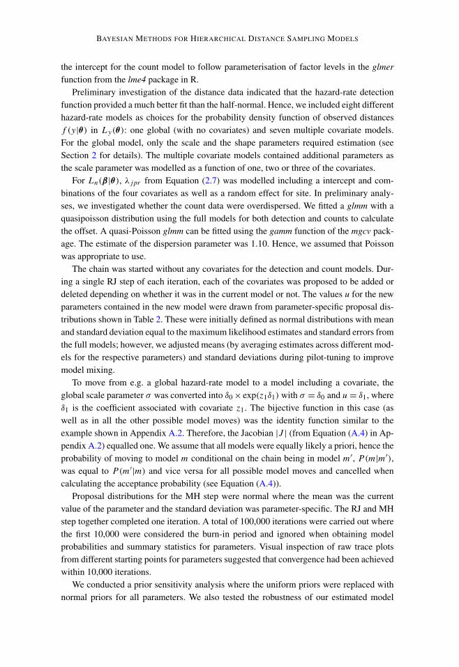
The chain was started without any covariates for the detection and count models. Dur-ing a single RJ step of each iteration, each of the covariates was proposed to be added ordeleted depending on whether it was in the current model or not. The values u for the newparameters contained in the new model were drawn from parameter-specific proposal dis-tributions shown in Table 2. These were initially defined as normal distributions with meanand standard deviation equal to the maximum likelihood estimates and standard errors fromthe full models; however, we adjusted means (by averaging estimates across different mod-els for the respective parameters) and standard deviations during pilot-tuning to improvemodel mixing.

To move from e.g. a global hazard-rate model to a model including a covariate, theglobal scale parameter σ was converted into δ0 × exp(z1δ1) with σ = δ0 and u = δ1, whereδ1 is the coefficient associated with covariate z1. The bijective function in this case (aswell as in all the other possible model moves) was the identity function similar to theexample shown in Appendix A.2. Therefore, the Jacobian |J | (from Equation (A.4) in Ap-pendix A.2) equalled one. We assume that all models were equally likely a priori, hence theprobability of moving to model m conditional on the chain being in model m′, P(m|m′),was equal to P(m′|m) and vice versa for all possible model moves and cancelled whencalculating the acceptance probability (see Equation (A.4)).

Proposal distributions for the MH step were normal where the mean was the currentvalue of the parameter and the standard deviation was parameter-specific. The RJ and MHstep together completed one iteration. A total of 100,000 iterations were carried out wherethe first 10,000 were considered the burn-in period and ignored when obtaining modelprobabilities and summary statistics for parameters. Visual inspection of raw trace plotsfrom different starting points for parameters suggested that convergence had been achievedwithin 10,000 iterations.

We conducted a prior sensitivity analysis where the uniform priors were replaced withnormal priors for all parameters. We also tested the robustness of our estimated model

C.S. OEDEKOVEN ET AL.

Table 2. Mean and standard deviation (SD) of Normal proposal distributions for parameters proposed to beadded or deleted during the RJ step of the RJMCMC algorithm. All parameters were categorical, exceptfor continuous Julian day.

Parameters Mean SD

Detection ModelYear level 2006 0.11 0.10Year level 2007 −0.15 0.10Type level: Control 0.50 0.10State level: GA 0.42 0.10State level: IA 0.21 0.10State level: IL 0.70 0.10State level: IN 0.67 0.10State level: KY 0.64 0.10State level: MO 0.69 0.10State level: MS 0.61 0.10State level: NC 0.66 0.10State level: SC 0.03 0.10State level: TN 0.47 0.10

Count ModelYear level: 2007 0.16 0.05Year level: 2008 0.08 0.05Type level: Treatment 0.42 0.10Julian Day: −0.01 0.01State level: IA 0.71 0.24State level: IL −0.49 0.24State level: IN −1.16 0.23State level: KY −0.41 0.22State level: MO 0.01 0.20State level: MS −0.38 0.22State level: NC −1.36 0.23State level: SC 0.07 0.22State level: TN −1.05 0.23State level: TX 1.77 0.21

probabilities by starting the RJMCMC algorithm from the full detection and count models(as opposed to the intercept only models). Both analyses revealed nearly identical resultsas those presented in Section 4.4. Hence, we were confident that our results had converged.

4.3. THE CLASSICAL APPROACH

To compare the Bayesian approach with the classical, the data were analysed usingthe two-stage approach (Buckland et al. 2009), extended to include a random effect forsite in the count model (Oedekoven et al. 2013). The first step included fitting a detectionfunction to observed distances by maximising the likelihood in Equation (2.3). The sameeight hazard-rate models were explored as in the Bayesian approach, i.e. global and MCDSmodels with combinations of the covariates state, type and year. The effective area νjpr

was estimated using the best model for f (y|θ).In a second step, the effective area was incorporated into the count model for λjpr and

parameter estimates obtained using the glmer function of the lme4 package (Bates 2009b)

BAYESIAN METHODS FOR HIERARCHICAL DISTANCE SAMPLING MODELS

Table 3. Models and their probabilities resulting from RJMCMC and bootstrap analyses. Each density modelincluded an intercept and a random effect for site in addition to shown covariates (JD = Julian day).Model probabilities refer to the percentage the respective models were chosen during 90 000 iterations(after 10 000 iterations of burn-in) for RJMCMC and during 999 bootstrap iterations.

Model RJMCMC Two-Stage

Detection ModelMCDS: Type <0.001 –MCDS: State – 0.01MCDS: Year + State – 0.16MCDS: Type + State <0.001 0.02MCDS: Year + Type + State 1.00 0.81Count ModelType + State – <0.005Year + Type + State – 0.01Type + JD + State 0.89 0.10Year + Type + JD + State 0.11 0.89

in R. The likelihood for the glmer function is equivalent to Equation (2.8), except that therandom effect is integrated out using an approximation for the integral (Bates 2009a). Thesame 16 models were explored as in the Bayesian approach, including a fixed intercept anda random effect for site and combinations of the four covariates state, type, year and Julianday.

Best fitting models for both steps were found by minimum AIC values. As the effectivearea represents an estimate but is included in the model as if it was a known constant, non-parametric bootstrapping was used to estimate uncertainty (bootstrap standard errors (BSE)and 95 % confidence intervals) of parameter estimates. To implement a non-parametricbootstrap routine with 999 repeats, an automatic model selection was set up in R thatincluded calls to the MCDS engine from the Distance software (Thomas et al. 2010) forthe first step. For each bootstrap iteration, sites were resampled with replacement until theoriginal number of sites was obtained (Buckland et al. 2009). To include model uncertaintyin inference, the strategy followed was to select best fitting models based on minimum AICvalues for each bootstrap iteration (Buckland, Burnham, and Augustin 1997).

4.4. RESULTS

In the following we refer to those models with highest probabilities as the preferredmodels. For the Bayesian approach, the preferred detection function model included thecovariates year, type and state in the model for the scale parameter of the hazard-ratekey function (probability = 1.00 to two decimal places, Table 3). Two other models werevisited within the RJMCMC algorithm with probabilities of <0.001 that included two(type and state) or one covariate only (type). The same model with all three covariateswas the preferred model for the two-stage approach having been selected by AIC in 81 %of bootstrap resamples. Three other models were selected: one with covariates year andstate (16 %), one with type and state (2 %) and one with state alone (1 %).

For the count model, two models dominated the RJMCMC algorithm, the model withcovariates type, Julian day and state as the preferred model (0.89 probability) and the full

C.S. OEDEKOVEN ET AL.

model (year + type + Julian day + state, 0.11 probability, Table 3). For the bootstrap,the latter was the preferred model, selected in 89 % of resamples, while the former wasthe second most frequently chosen model (10 %). Two other models were chosen duringthe bootstrap, the model including the covariates year, type and state (1 %) and the modelincluding covariates type and state (<1 %). Hence, the largest discrepancy in model prob-abilities between the two analysis methods was with regard to covariate year for whichthe total probabilities to be included in any model was 0.11 for the RJMCMC algorithmand 0.90 for the bootstrap (Table 3). However, 95 % confidence intervals obtained from thebootstrap overlapped zero for both year coefficients (Table 4), indicating that this covariatemight have less importance than suggested by model probabilities for the bootstrap.

For the parameters of the detection function model, the posterior means of the parame-ters in the preferred model were in most cases similar to the maximum likelihood estimatesresulting from the two-stage analysis of the original data (Table 4). The intercept for thescale parameter and the shape parameter were larger for the Bayesian approach, whilethe coefficients for the scale parameter were on average smaller. Histograms of detectionsby state and estimated expected probability density functions (pdf) of observed distancesfrom the Bayesian approach are shown in Fig. 1. States SC and TX had the lowest averagedetection probabilities as indicated by the smallest coefficients for these states (Table 4).For these states, the steep decline after peak values for the pdf indicated rapidly decliningdetection probabilities beyond ∼100 m (Fig. 1).

Interestingly, measures of uncertainty were mostly smaller for the Bayesian approachdespite the fact that both stages from the two-stage approach were combined in one. Theposterior standard deviations were smaller than the bootstrap standard errors for all detec-tion function parameters. The 95 % credible intervals were narrower than the 95 % con-fidence intervals for all but four detection function parameters (state coefficients IN, MS,NC and TN). Intervals from the two approaches overlapped in all cases for the detectionfunction parameters.

For the count model, means and intervals were again similar between the two ap-proaches (Table 4). However, slight discrepancies in means for count model coefficientsexisted, which might have been due to that the best model from the two-stage approachcontained the additional covariate year and/or to Monte Carlo error. Further reasons arediscussed in Section 5. Also, measures of uncertainty were again mostly smaller for theBayesian approach: standard deviations from the Bayesian approach were smaller for allcovariates in the count model compared to BSEs. The 95 % credible intervals were nar-rower for all coefficients of the count model compared to the 95 % confidence intervals,except for the covariate Julian day where they were equal. The 95 % credible and confi-dence intervals overlapped for all count model parameters. The only covariate selected forthe preferred count model for the two-stage approach that was not also in the preferredmodel for the Bayesian approach was year. The 95 % confidence intervals for both yearcoefficients included zero, indicating that this covariate might have been negligible for thecount model.

The parameter of interest in these models was the coefficient for the level Treatmentof the type covariate in the count model. This was 0.62 (SD = 0.07) and 0.63 (BSE =

BAYESIAN METHODS FOR HIERARCHICAL DISTANCE SAMPLING MODELS

Table 4. Mean, standard deviation (SD) and 95 % credible intervals (CRI) from the RJMCMC analysis alongwith maximum likelihood estimates (MLE), bootstrap standard errors (BSE) and 95 % confidenceintervals (CI) using the two-stage approach for the models with the highest probabilities (see Table3 for model probabilities). Units of measurements were metres for the detection function model andsquare metres for the count model.

RJMCMC Two-Stage

Mean SD 95 % CRI MLE BSE 95 % CI

Detection ModelScale Intercept 152.96 8.97 135.47, 170.12 138.59 16.13 112.26, 163.79Shape 3.30 0.16 3.00, 3.63 3.01 0.27 2.68, 3.41Scale: Year 2006 0.06 0.03 0.01, 0.12 0.10 0.06 −0.05, 0.14Scale: Year 2007 −0.11 0.04 −0.19, −0.05 −0.15 0.05 −0.25, -0.1Scale: Type Control 0.13 0.04 0.05, 0.20 0.15 0.05 0.05, 0.23Scale: State GA 0.38 0.07 0.23, 0.52 0.42 0.17 0.05, 0.54Scale: State IA 0.17 0.10 −0.01, 0.36 0.21 0.16 −0.12, 0.30Scale: State IL 0.66 0.09 0.48, 0.85 0.70 0.17 0.35, 0.76Scale: State IN 0.62 0.10 0.43, 0.81 0.66 0.14 0.34, 0.72Scale: State KY 0.58 0.08 0.43, 0.74 0.64 0.12 0.35, 0.68Scale: State MO 0.62 0.06 0.51, 0.73 0.69 0.09 0.46, 0.71Scale: State MS 0.55 0.07 0.41, 0.70 0.61 0.10 0.37, 0.64Scale: State NC 0.60 0.09 0.43, 0.79 0.66 0.12 0.35, 0.70Scale: State SC 0.01 0.08 −0.14, 0.16 3E–5 0.14 −0.29, 0.12Scale: State TN 0.44 0.10 0.25, 0.63 0.47 0.12 0.19, 0.54Count Model: Random EffectsStandard deviation 0.82 0.05 0.73, 0.91 0.78 0.04 0.69, 0.81Count Model: CoefficientsIntercept Density −13.10 0.18 −13.43, −12.73 −13.23 0.33 −13.91,−12.87Year 2007 – – – 0.17 0.13 −0.16, 0.37Year 2008 – – – 0.17 0.11 −0.12, 0.31Type Treatment 0.62 0.07 0.48, 0.75 0.63 0.12 0.36, 0.71Julian Day −0.01 2E–3 −0.02, −0.01 −0.01 3E–3 −0.02, −0.01State IA −0.81 0.29 −1.38, −0.23 −0.74 0.44 −1.65, −0.24State IL −0.59 0.27 −1.12, −0.06 −0.53 0.38 −1.25, −0.07State IN −1.24 0.27 −1.79, −0.71 −1.18 0.41 −1.99, −0.70State KY −0.47 0.25 −0.98, 0.03 −0.44 0.34 −1.07, −0.02State MO 0.01 0.22 −0.44, 0.42 0.05 0.34 −0.63, 0.46State MS −0.43 0.25 −0.92, 0.05 −0.37 0.34 −1.04, 0.05State NC −1.39 0.26 −1.88, −0.87 −1.31 0.36 −1.99, −0.87State SC 0.01 0.27 −0.53, 0.53 0.08 0.42 −0.76, 0.56State TN −1.10 0.28 −1.65, −0.57 −1.03 0.38 −1.80, −0.60State TX 1.74 0.18 1.33, 1.99 1.46 0.29 0.99, 1.81

0.12) for the Bayesian and the two-stage approach, respectively, indicating an increasein covey densities on treatment plots by 85 % (E[exp(type coefficient)] = 1.85) or 88 %(exp(0.63) = 1.88) by the respective methods.

As described above, the expected densities can be calculated using the values of the β

parameters from the count model. These values are obtained from the posterior distribu-tion of these parameters for the Bayesian approach or maximum likelihood estimates forthe two-stage approach (see above Equations (2.6) and (2.7) for details). For calculatingbaseline estimates of the expected covey densities for the RJMCMC algorithm and two-stage approach, we used those iterations from the respective methods where the preferred

C.S. OEDEKOVEN ET AL.

Figure 1. Estimated probability density functions, f (y) (y-axis), using mean parameter values from theBayesian approach (Table 4) against radial distance from the point (x-axis, in metres), and histograms of de-tections for each of 11 states (GA, IA, IL, IN, KY, MO, MS, NC, SC, TN, TX); here, n represents the number ofdetections for the respective states. For each state, f (y) was averaged over all levels of covariates year and type.

count model was chosen, excluding the burn-in iterations for the RJMCMC. Using Equa-tion (2.7), we set the covariates to those levels that were absorbed by the intercept of thedensity model, i.e. year = 2006, type = Control, Julian day = 0 (which is equivalent toits mean as we centred the data for this covariate) and state = GA and added a randomeffect contribution (0.5 × σb

2 replaces bj from Equation (2.7) when calculating the aver-

BAYESIAN METHODS FOR HIERARCHICAL DISTANCE SAMPLING MODELS

Figure 2. Estimated covey densities (coveys per km2) and 95 % CRIs for each of 11 states shown for unbufferedcontrol and buffered treatment fields.

age expected density across all sites). The estimated baseline expected density from theRJMCMC algorithm was 2.91 coveys per km2 (SD = 0.55, 95 % CRI = (2.05, 4.14)). Theposterior distribution of the expected density was right-skewed with a mode of 2.60 coveysper km2. The estimated expected density resulting from the two-stage approach was 2.44coveys per km2 (BSE = 0.88, 95 % CI = (1.25, 4.66)). The estimated expected densitiesfor each state and type combination are shown in Fig. 2.

5. DISCUSSION

There are two main aspects in this paper that are innovative and deserve comparison toexisting methods. We present a novel approach for combining the likelihood functions foranalysing distance sampling data in Section 2, which is easily applicable to both intervaland exact distance data. We also present a Bayesian approach for analysing distance sam-pling data of multiple types in a straightforward manner. Different detection functions (thehalf-normal, hazard-rate or others) may easily be implemented. It may also be extended toinclude adjustment terms (added to the half-normal or hazard-rate model, Buckland et al.2001) or covariates in the shape parameter. We provide the R code as online supplementarymaterial, which is annotated for easy adaptation.

Bayesian methods have been used before for analysing line transect data with a globalhalf-normal detection function (e.g. Royle and Dorazio 2008, Chapter 7.1; Eguchi andGerrodette 2009; Gimenez et al. 2009; Zhang 2011), a half-normal with covariates (e.g.Gerrodette and Eguchi 2011; Moore and Barlow 2011) or a hazard-rate with one covariate(Schmidt et al. 2012). Our approach allows simultaneous exploration of model and pa-rameter space including different detection functions and different covariate combinations

C.S. OEDEKOVEN ET AL.

for both the detection and count models via an RJMCMC algorithm. Conn, Laake, andJohnson (2012) described an RJMCMC algorithm for distance sampling data. However,in their case, the RJ step refers to adding/deleting unobserved animals as part of the dataaugmentation and not to exploring different models for the detection function or counts.

The log-linear Poisson model for counts described in Section 2 does not depend on arandom survey design in contrast with the classical distance sampling approach and dataarising from surveys conducted from platforms of opportunity may be used (Hedley andBuckland 2004). It allows identification of relationships between abundance or density andparameters of interest, such as the type covariate in our case study, which may be of interestfor designed experiments and wildlife management studies (see also Gerrodette and Eguchi2011). Similar to Hedley and Buckland (2004) and Buckland et al. (2009), our count modelmay be extended to include smooth functions for continuous covariates, e.g. by fittingpolynomial splines using the B-spline basis, or the Poisson likelihood may be replacedwith a negative binomial likelihood if more appropriate, e.g. in case overdispersion in thecount data is present (e.g. Royle, Dawson, and Bates 2004, Sillett et al. 2012).

Our approach is similar to Hedley and Buckland (2004) in that we use the conditionalformulation of the probability density function of observed distances (Buckland et al. 2001)and information on detection probabilities enters the count model via an offset; we modelcounts as density × effective area. However, Hedley and Buckland (2004) or Bucklandet al. (2009) analyse their data in two stages. In their second stage count model, theycondition on the estimate of the effective area derived from the first stage detection model.This requires conducting non-parametric bootstrapping so that uncertainty associated withestimating the detection function (and the effective area) propagates into the second stagecount model. Our integrated likelihood approach estimates all parameters simultaneously,allowing direct quantification of the precision of the parameters in the count model withtaking proper account of the estimation of detection function parameters.

Using the Poisson model with a random effect for estimating densities as defined inEquation (2.7) also allows us to accommodate correlated measurements due to closenessin space and/or time, as occurs e.g. when there are repeat counts at the same line (point).This differs from the integrated likelihood described by Royle, Dawson, and Bates (2004).These authors considered the true but unknown abundances at the site as a random effectwith a Poisson distribution (in their notation Ni ∼ Poisson(λi)) and integrate it out by sum-mation. They derive a Poisson likelihood for the observed counts with expected value equalto λiπk(θ), where πk(θ) is obtained using the unconditional probability density functionof observed distances and describes the probability that an animal occurs and is detectedin the kth distance interval. Hence, these authors model counts as abundance N × de-tected proportion of N for each interval. Note that we use the term integrated likelihoodin the spirit of integrating the likelihood components pertaining to two different data types(described in Section 2), while Royle, Dawson, and Bates (2004) use the same term inthe context of integrating out a nuisance parameter (although they combine the likelihoodcomponents from two different data sources as well).

In contrast to Royle, Dawson, and Bates (2004), we model variations in observed countsbetween the different sites (those variations not explained by any of the fixed effects in-

BAYESIAN METHODS FOR HIERARCHICAL DISTANCE SAMPLING MODELS

cluded in the model) as a normally distributed random effect with mean zero, hence ac-counting for correlations between measurements at the same sites. This represents an ex-tension to Royle, Dawson, and Bates who include one count per site in the analysis. Withthe inclusion of site random effects, our approach allows us to incorporate repeat countsfrom the same sites in the analysis. Our approach assumes that all counts from the samesite are positively correlated and only requires estimation of one additional parameter, therandom effect standard deviation. Chelgren et al. (2011), on the other hand, extended theapproach of Royle, Dawson, and Bates (2004) by including a random effect for plot byweek in the abundance model which requires estimation of week-specific variance param-eters. However, including random effects allows inference on the wider area that these sitesrepresent and to obtain unbiased estimates of coefficients retained in the count model. Biasin coefficient estimates may occur for example if some sites with high bird densities werevisited more frequently than those with low densities, and this variation was not modelledas a fixed or random effect.

The comparison of summary statistics for model parameters from the Bayesian ap-proach with those from the two-stage approach revealed some differences in means andpoint estimates (Table 4) which cannot be due to prior sensitivity as we used uniform pri-ors on all parameters for the Bayesian approach. We assume that these differences mayhave been due to the fact that—as opposed to the two-stage approach—the likelihoodsfor both components of our model were combined for the integrated likelihood and influ-ence each other. We argue, in concurrence with Johnson, Laake, and Ver Hoef (2010), thatsimultaneous estimation of all parameters in one stage represents a more realistic modelwithout having to rely on the assumption of a true detection function model. Whether thesmaller uncertainty estimates from the Bayesian approach compared to the two-stage ap-proach were specific to our case study or can be expected in general is beyond the scope ofthis paper.

Our Bayesian approach provides improvements over previous approaches. Besides theoften stated benefits for Bayesian analyses, e.g. allowing for prior information to be in-cluded, our Bayesian approach provided a particular benefit for using the integrated likeli-hood defined in Section 2: it might be challenging in some cases, such as our case study, tofind the maximum likelihood estimates for all parameters in one step. The covey data in-cluded a total of 2545 observed distances during 2534 counts, and the full model included31 parameters with a random effect (447 sites). Using maximum likelihood methods, therandom effect coefficients are not estimated individually but are integrated out during theoptimisation of the likelihood. However, due to the integrated nature of the detection anddensity models, functions such as glmer from the lme4 package in R may not be used asthese treat the offset as a constant. Using the hierarchical model set up for the Bayesian ap-proach, the random effect coefficients are included in the model specification and updatedduring each iteration. Due to this data augmentation method, no numerical integration isnecessary providing a straightforward technique to explore the parameter space.

Bayesian methods also offer efficient exploration of model space with the use of RJM-CMC. By contrast, using a maximum likelihood approach, a model selection routine thatconsidered all possible model combinations for our case study would have required max-imising Ly,n(β, θ) for 128 models (possible combinations of eight detection functions and

C.S. OEDEKOVEN ET AL.

16 count models). RJMCMC, on the other hand, allows incorporating model uncertaintyinto a single chain.

APPENDIX

A.1 Metropolis–Hastings

We use a single-update random walk MH algorithm where we cycle through each parame-ter in Ln,y(β, θ). To use a simple scenario, assume that β = {β0, σb}. Then, e.g. for param-eter β0 with current value βt

0, we propose to move to a new state, β ′0, with β ′

0 ∼ (βt0, σ

2β0

).This newly proposed state is accepted as the new state with probability α(β ′

0|βt0) given by

α(β ′

0

∣∣ βt

0

) = min

(

1,Ln,y(β

′0, σ

tb, θ

t )p(β ′0)q(βt

0|β ′0)

Ln,y(βt0, σ

tb, θ

t )p(βt0)q(β ′

0|βt0)

)

. (A.1)

Here, q(β ′0|βt

0) denotes the proposal density of β ′0 given the current state is βt

0. We notethat the terms q(βt

0|β ′0) and q(β ′

0|βt0) cancel in the acceptance probability since we use a

symmetrical proposal distribution. The analogous MH updates are used for random effectcoefficients. Proposal variances are chosen via pilot-tuning.

A.2 Model Selection: Reversible Jump MCMC

The joint posterior distribution of models and parameters is given (up to proportionality)by

πn,y(βm, θm,m) ∝ Ln,y(βm, θm,m)p(βm, θm|m)p(m), (A.2)

where Ln,y(βm, θm,m) denotes the probability density function of the data given currentparameter values βm and θm and model m, p(βm, θm|m) the prior distribution for modelparameters βm and θm, and p(m) the prior probability of model m. The RJMCMC algo-rithm is used to explore the parameter and model space simultaneously (Green 1995).

Each iteration involves two steps: a within model move and a between model move.During the within model move, the Metropolis–Hastings (MH) algorithm is used to updatethe parameters given the model (as described above in Section 3.2). During the betweenmodel move, the reversible jump (RJ) step, model m conditional on the current parametervalues is updated. This move involves a proposal to update the model itself; suppose thechain is in model m and we propose to move to model m′. A bijective function describes therelationship between the current and proposed parameters and is used to convert parametersfrom model m to parameters for model m′. In a simple scenario, say, where model m

contains parameters β = {β0, β1} and model m′ contains parameters β ′ = {β ′0, β

′2}, the

bijective function might be expressed as an identity function:

β ′0 = β0 u′ = β1 β ′

2 = u. (A.3)

BAYESIAN METHODS FOR HIERARCHICAL DISTANCE SAMPLING MODELS

Here u and u′ are random samples from some proposal distributions for the respectiveparameters. The acceptance probability may then be expressed as

A = πn,y(β′,m′)P (m|m′)q ′(u′)

πn,y(β,m)P (m′|m)q(u)|J |, (A.4)

where P(m′|m) denotes the probability of proposing to move to model m′ given that thechain is in model m, q(u) and q ′(u′) are the proposal densities of u and u′, and |J | is theJacobian (which equals one if the bijective function is the identity function).

ACKNOWLEDGEMENTS

The National CP-33 Monitoring Program was coordinated and delivered by the Department of Wildlife, Fish-eries, and Aquaculture and the Forest and Wildlife Research Center, Mississippi State University and funded bythe Multistate Conservation Grant Program (Grant MS M-1-T), which is supported by the Wildlife and Sport FishRestoration Program and managed by the Association of Fish and Wildlife Agencies and US Fish and WildlifeService. Further support was provided by the US Department of Agriculture (USDA) Farm Service Agency andUSDA Natural Resources Conservation Service Conservation Effects Assessment Project. Collaborators includedthe AR Game and Fish Commission, GA Department of Natural Resources (DNR), IL DNR/Ballard Nature Cen-ter, IN DNR, IA DNR, KY Department of Fish and Wildlife Resources/KY Chapter of The Wildlife Society, MSDepartment of Wildlife, Fisheries and Parks, MO Department of Conservation, NE Game and Parks Commission,NC Wildlife Resources Commission, OH DNR, SC DNR, TN Wildlife Resources Agency, TX Parks and WildlifeDepartment, Southeast Quail Study Group and Southeast Partners In Flight. Cornelia S. Oedekoven was supportedby a studentship jointly funded by the University of St Andrews and EPSRC (EPSRC grant EP/C522702/1),through the National Centre for Statistical Ecology. Some of the R functions for the two-stage approach wereprovided by Len Thomas.

[Received May 2013. Accepted January 2014.]

REFERENCES

Bates, D. (2009a), “Adaptive Gauss–Hermite Quadrature for Generalized Linear or Nonlinear Mixed Models. RPackage Version 0.999375-31,” Technical Report. http://lme4.r-forge.r-project.org/.

Bates, D. (2009b), “Computational Methods for Mixed Models. R Package Version 0.999375-31,” TechnicalReport. http://lme4.r-forge.r-project.org/.

Buckland, S. T., Burnham, K. P., and Augustin, N. H. (1997), “Model Selection: An Integral Part of Inference,”Biometrics, 53 (2), 603–618.

Buckland, S. T., Goudie, I. B. J., and Borchers, D. L. (2000), “Wildlife Population Assessment: Past Develop-ments and Future Directions,” Biometrics, 56, 1–12.

Buckland, S. T., Anderson, D. R., Burnham, K. P., Laake, J. L., Borchers, D. L., and Thomas, L. (2001), Intro-

duction to Distance Sampling, London: Oxford University Press.

Buckland, S. T., Anderson, D. R., Burnham, K. P., Laake, J. L., Borchers, D. L., and Thomas, L. (2004), Advanced

Distance Sampling, London: Oxford University Press.

Buckland, S. T., Russell, R. E., Dickson, B. G., Saab, V. A., Gorman, D. G., and Block, W. M. (2009), “AnalysingDesigned Experiments in Distance Sampling,” Journal of Agricultural, Biological, and Environmental Statis-

tics, 14, 432–442.

Cañadas, A., and Hammond, P. S. (2006), “Model-Based Abundance Estimates for Bottlenose Dolphins offSouthern Spain: Implications for Conservation and Management,” Journal of Cetacean Research and Man-

agement, 8 (1), 13–27.

C.S. OEDEKOVEN ET AL.

Chelgren, N. D., Samora, B., Adams, M. J., and McCreary, B. (2011), “Using Spatiotemporal Models and Dis-tance Sampling to Map the Space Use and Abundance of Newly Metamorphosed Western Toads (AnaxyrusBoreas),” Herpetological Conservation and Biology, 6 (2), 175–190.

Conn, P. B., Laake, J. L., and Johnson, D. S. (2012), “A Hierarchical Modeling Framework for Multiple ObserverTransect Surveys,” PLoS ONE, 7 (8), e42294.

Davison, A. C. (2003), Statistical Models, Cambridge: Cambridge University Press.

Durban, J. W., and Elston, D. A. (2005), “Mark-Recapture with Occasion and Individual Effects: AbundanceEstimation Through Bayesian Model Selection in a Fixed Dimensional Parameter Space,” Journal of Agri-

cultural, Biological, and Environmental Statistics, 10 (3), 291–305.

Eguchi, T., and Gerrodette, T. (2009), “A Bayesian Approach to Line-Transect Analysis for Estimating Abun-dance,” Ecological Modelling, 220, 1620–1630.

Evans, K. O., Burger, L. W., Oedekoven, C. S., Smith, M. D., Riffell, S. K., Martin, J. A., and Buckland, S. T.(2013), “Multi-Region Response to Conservation Buffers Targeted for Northern Bobwhite,” The Journal of

Wildlife Management, 77, 716–725.

Gelman, A., Roberts, G. O., and Gilks, W. R. (1996), “Efficient Metropolis Jumping Rules,” in Bayesian Statistics,Vol. 5, eds. M. Bernardo, J. O. Berger, A. P. Dawid, and A. F. M. Smith, Oxford: Oxford University Press,pp. 599–608.

Gerrodette, T., and Eguchi, T. (2011), “Precautionary Design of a Marine Protected Area Based on a HabitatModel,” Endangered Species Research, 15 (2), 159–166.

Gimenez, O., Bonner, S. J., King, R., Parker, R. A., Brooks, S. P., Jamieson, L. E., Grosbois, V., Morgan, B. J.T., and Thomas, L. (2009), “WinBUGS for Population Ecologists: Bayesian Modeling Using Markov ChainMonte Carlo Methods,” in Modeling Demographic Processes in Marked Populations. Environmental and

Ecological Statistics, Vol. 3, eds. D. L. Thomson, E. G. Cooch, and M. J. Conroy, Berlin: Springer, pp. 883–915.

Green, P. J. (1995), “Reversible Jump Markov Chain Monte Carlo Computation and Bayesian Model Determina-tion,” Biometrika, 82 (4), 711–732.

Hastings, W. K. (1970), “Monte Carlo Sampling Methods Using Markov Chains and Their Applications,”Biometrika, 57 (1), 97–109.

Hedley, S. L., and Buckland, S. T. (2004), “Spatial Models for Line Transect Sampling,” Journal of Agricultural,

Biological, and Environmental Statistics, 9, 181–199.

Johnson, D. S., Laake, J. L., and Ver Hoef, J. M. (2010), “A Model-Based Approach for Making EcologicalInference from Distance Sampling Data,” Biometrics, 66, 310–318.

Karunamuni, R. J., and Quinn II., T. J. (1995), “Bayesian Estimation of Animal Abundance for Line TransectSampling,” Biometrics, 51, 1325–1337.

King, R., Morgan, B. J. T., Gimenez, O., and Brooks, S. P. (2010), Bayesian Analysis for Population Ecology,London/Boca Raton: Chapman & Hall/CRC Press.

Marcot, B. G., Holthausen, R. S., Raphael, M. G., Rowland, M. M., and Wisdom, M. J. (2001), “Using BayesianBelief Networks to Evaluate Fish and Wildlife Population Viability Under Land Management Alternativesfrom an Environmental Impact Statement,” Forest Ecology and Management, 153, 29–42.

Marques, F. F. C., and Buckland, S. T. (2003), “Incorporating Covariates Into Standard Line Transect Analyses,”Biometrics, 53, 924–935.

McCulloch, C. E., and Searle, S. R. (2001), Generalized, Linear, and Mixed Models, New York: Wiley.

Metropolis, N., Rosenbluth, A. W., Rosenbluth, M. N., Teller, A. H., and Teller, E. (1953), “Equations of StateCalculations by Fast Computing Machines,” Journal of Chemical Physics, 21 (6), 1087–1091.

Moore, J. E., and Barlow, J. (2011), “Bayesian State-Space Model of Fin Whale Abundance Trends from a 1991–2008 Time Series of Line-Transect Surveys in the California Current,” Journal of Applied Ecology, 48 (5),1195–1205.

Oedekoven, C. S., Buckland, S. T., Mackenzie, M. L., Evans, K. O., and Burger, L. W. (2013), “ImprovingDistance Sampling: Accounting for Covariates and Non-independency Between Sampled Sites,” Journal of

Applied Ecology, 50 (3), 786–793.

BAYESIAN METHODS FOR HIERARCHICAL DISTANCE SAMPLING MODELS

Royle, J. A., and Dorazio, R. M. (2008), Hierarchical Modeling and Inference in Ecology: The Analysis of Data

from Populations, Metapopulations and Communities, San Diego: Academic Press.

Royle, J. A., Dawson, D. K., and Bates, S. (2004), “Modelling Abundance Effects in Distance Sampling,” Ecol-

ogy, 85 (6), 1591–1597.

Schmidt, J. H., Lindberg, M. S., Johnson, D. S., Conant, B., and King, J. (2009), “Evidence of Alaskan TrumpeterSwan Population Growth Using Bayesian Hierarchical Models,” The Journal of Wildlife Management, 73 (5),720–727.

Schmidt, J. H., Rattenbury, K. L., Lawler, J. P., and MacCluskie, M. C. (2012), “Using Distance Sampling andHierarchical Models to Improve Estimates of Dall’s Sheep Abundance,” The Journal of Wildlife Management,76 (2), 317–327.

Sillett, T. S., Chandler, R. B., Royle, J. A., Kéry, M., and Morrison, S. A. (2012), “Hierarchical Distance-SamplingModels to Estimate Population Size and Habitat-Specific Abundance of an Island Endemic,” Ecological Ap-

plications, 22, 1997–2006.

Thomas, L., Buckland, S. T., Rexstad, E. A., Laake, J. L., Strindberg, S., Hedley, S. L., Bishop, J. R. B., Marques,T. A., and Burnham, K. P. (2010), “Distance Software: Design and Analysis of Distance Sampling Surveysfor Estimating Population Size,” Journal of Applied Ecology, 47, 5–14.

Zhang, S. (2011), “On Parametric Estimation of Population Abundance for Line Transect Sampling,” Environ-

mental and Ecological Statistics, 18, 79–92.