Bayesian Isotonic Regression and Trend...
25
Bayesian Isotonic Regression and Trend Analysis Brian Neelon 1,* and David B. Dunson 2 June 9, 2003 1 Department of Biostatistics, University of North Carolina, Chapel Hill, NC 2 Biostatistics Branch, MD A3-03, National Institute of Environmental Health Sciences P.O. Box 12233, Research Triangle Park, NC 27709 * email: [email protected] 1
Transcript of Bayesian Isotonic Regression and Trend...

Bayesian Isotonic Regression and Trend Analysis
Brian Neelon1,∗ and David B. Dunson2
June 9, 2003
1 Department of Biostatistics, University of North Carolina, Chapel Hill, NC
2 Biostatistics Branch, MD A3-03, National Institute of Environmental Health Sciences
P.O. Box 12233, Research Triangle Park, NC 27709
∗email: [email protected]
1

SUMMARY. In many applications, the mean of a response variable can be assumed to be
a non-decreasing function of a continuous predictor, controlling for covariates. In such cases,
interest often focuses on estimating the regression function, while also assessing evidence
of an association. This article proposes a new framework for Bayesian isotonic regression
and order restricted inference based on a constrained piecewise linear model with unknown
knot locations, corresponding to thresholds in the regression function. The non-decreasing
constraint is incorporated through a prior distribution consisting of a product mixture of
point masses (accounting for flat regions) and truncated autoregressive normal densities.
An MCMC algorithm is used to obtain a smooth estimate of the regression function and
posterior probabilities of an association for different regions of the predictor. Generalizations
to categorical outcomes and multiple predictors are described, and the approach is applied
to data from a study of pesticide exposure and birth weight.
KEY WORDS: Additive model; Autoregressive prior; Constrained estimation; Model aver-
aging; Monotonicity; Order restricted inference; Threshold model; Trend test.
2

1. Introduction
In many applications, the mean of a response variable, Y , conditional on a predictor, X,
can be characterized by an unknown isotonic function, f(·), and interest focuses on (i)
assessing evidence of an overall increasing trend; (ii) investigating local trends (e.g., at low
dose levels); and (iii) estimating the response function, possibly adjusted for the effects of
covariates, Z. For example, in epidemiologic studies, one may be interested in assessing the
relationship between dose of a possibly toxic exposure and the probability of an adverse
response, controlling for confounding factors. In characterizing biologic and public health
significance, and the need for possible regulatory interventions, it is important to efficiently
estimate dose response, allowing for flat regions in which increases in dose have no effect.
In such applications, one can typically assume a priori that an adverse response does not
occur less often as dose increases, adjusting for important confounding factors, such as age
and race. It is well known that incorporating such monotonicity constraints can improve
estimation efficiency and power to detect trends (Robertson, Wright, and Dykstra, 1988).
Motivated by these advantages and by the lack of a single framework for isotonic dose
response estimation and trend testing, accounting for covariates and flat regions, this article
proposes a Bayesian approach.
Consider a regression model, where a response Y is linked to a vector of covariates X =
(x1, . . . , xp)′ through an additive structure:
Y = α+p∑
l=1
fl(xl) + ε, (1)
where α is an intercept parameter, fl(·) is an unknown regression function for the lth covari-
ate, and ε is a zero-mean error residual. Additive models are appealing since they reduce the
problem of estimating a function of the p-dimensional predictor X to the more manageable
problem of estimating p univariate functions fl(·), one for each covariate xl.
3

There is a well developed literature on frequentist approaches for fitting additive models,
using a variety of methods to obtain smoothed estimates of each fl(·) (cf., Hastie and Tib-
shirani, 1990). In the Bayesian setting, Denison et al. (1998) and Holmes and Mallick
(2000) have proposed an approach for using piecewise linear splines for nonparametric curve
estimation. A prior distribution is placed on the number of knots and estimation proceeds
via reversible jump Markov chain Monte Carlo (MCMC) and least squares fitting. How-
ever, these methods do not incorporate monotonicity or shape restrictions on the regression
functions.
In the setting of estimating a potency curve, Gelfand and Kuo (1991) and Ramgopal, Laud,
and Smith (1993) proposed nonparametric Bayesian methods for dose response estimation
under strict constraints. Lavine and Mockus (1995) considered related methods for contin-
uous response data, allowing nonparametric estimation of the mean regression curve and
residual error density. These methods focus on estimation subject to strict monotonicity
constraints, and cannot be used directly for inferences on flat regions of the dose response
curve.
To address this problem, Holmes and Heard (2003) recently proposed an approach for
Bayesian isotonic regression using a piecewise constant model with unknown numbers and
locations of knots. Posterior computation is implemented using a reversible jump MCMC
algorithm, which proceeds without considering the constraint. To assess evidence of a mono-
tone increasing dose response function, they compute Bayes factors based on the proportions
of draws from the unconstrained posterior and unconstrained prior for which the constraint
is satisfied. The resulting tests are essentially comparisons of the hypothesis of monotonicity
to the hypothesis of any other dose response shape.
This article proposes a fundamentally different approach, based on a piecewise linear model
4

with prior distributions explicitly specified to have support on the restricted space and to
allow flat regions of the dose response curve. The piecewise linear model allows one to
obtain an excellent approximation to most smooth monotone functions using only a few
knots, and we focus on comparing the null hypothesis of a flat dose response function to the
alternative that there is at least one increase. Our prior distribution for the slope parameters
takes the form of a product mixture of point masses at zero, which allow for flat regions,
and truncated autoregressive normal densities, and we allow for unknown number of knots
and knot locations. The structure of this prior, which is related to priors for Bayesian
variable selection in linear regression (Geweke, 1996; George and McCulloch, 1997), results
in simplified posterior computation.
Section 2 proposes the model, prior structure, and MCMC algorithm. Section 3 presents the
results from a simulation study. Section 4 applies the methods to data from an epidemiologic
study of pesticide exposure and birth weight, and Section 5 discusses the results.
2. The Model
2.1 Piecewise Linear Isotonic Regression
We focus initially on the univariate normal regression model,
yi = f(xi) + εi, i = 1, . . . , n, (2)
where f ∈ Θ+ is an unknown isotonic regression function, with
Θ+ = {f : f(x1) ≤ f(x2) ∀(x1, x2) ∈ <2 : x1 < x2}
denoting the space of non-decreasing functions, and εiiid∼ N(0, σ2) an error residual for the ith
subject. Modifications for f ∈ Θ−, the space of non-increasing functions, are straightforward.
5

We approximate f(·) using a piecewise linear model,
f(xi) ≈ β0 +k∑
j=1
wj(xi)βj = β0 +k∑
j=1
wijβj = w′iβ, j = 1, . . . , k, i = 1, . . . , n (3)
where β0 is an intercept parameter, wij = wj(xi; γ) = min(xi, γj) − γj−1 if xi ≥ γj−1 and
wij = 0 otherwise, γ = (γ0, . . . , γk)′ are knot locations (with xi ∈ [γ0, γk]∀i), βj is the slope
within interval (γj−1, γj], wi = (1, wi1, . . . , wik)′ and β = (β0, . . . , βk)
′.
The conditional likelihood of y = (y1, . . . yn)′ given θ = (β,γ)′, σ2 and x = (x1, . . . ,xn)′
can therefore be written as
L(y|θ, σ2,x) = (2πσ2)−n2 exp
{− 1
2σ2
n∑i=1
(yi −w′iβ)2
}. (4)
This likelihood can potentially be maximized subject to the constraint βj ≥ 0, for j =
1, . . . , k, to obtain estimates satisfying the monotonicity constraint. However, the resulting
restricted maximum likelihood estimates of the regression function will not be smooth, and
there can be difficulties in performing inferences, since the null hypothesis of no association
falls on the boundary of the parameter space.
2.2 Prior Specification and Model Averaging
We instead follow a Bayesian approach, choosing prior distributions for the parameters β
and γ. For simplicity in prior elicitation and computation, we assume a priori independence
between the different parameters, so that π(θ, σ2) = π(β)π(γ)π(σ2). For the error precision,
we choose a gamma conjugate prior, π(σ−2) = G(σ2; a, b), where a and b are investigator-
specified hyperparameters. For the regression parameters, β, we choose
π(β) = N(β0;µ0, λ20) ZI-N+(β1; π01, 0, λ
2)k∏
j=2
ZI-N+(βj; π0j, βj−1, λ2). (5)
Here, we use the ZI-N+(π0, µ, λ2) notation to denote a zero-inflated positive normal density—
i.e., a density consisting of the mixture of a point mass at zero, with probability π0, and a
6

N(µ, λ2) density truncated below by zero. In particular, we have
ZI-N+(z; π0, µ, λ2) = π01(z=0) + (1− π0)
1(z>0)N(z;µ, λ2)
Φ(µ/λ),
where Φ(z) =∫ z0
√2π exp(−s2) ds denotes the standard normal distribution function.
Prior (5) assigns probability Pr(βj = 0) = π0j to the case in which f(x) is flat in the jth in-
terval, (γj−1, γj], and Pr(βj > 0) = 1−π0j to the case in which f(x) is increasing. The special
case where β1 = · · · = βk = 0 corresponds to the global null hypothesis, H0 : f(x) is constant
for all x ∈ [γ0, γk]. Thus, the prior probability of H0 is π0 =∏k
j=1 π0j. The mean of the nor-
mal component of the mixture prior for βj is set equal to βj−1, allowing for autocorrelation
in the slopes, and λ is a hyperparameter measuring the degree of autocorrelation.
Prior density (5) is similar in structure to mixture priors proposed for variable selection
in linear regression (Geweke, 1996; Chipman, George and McCulloch, 2001; George and
McCulloch, 1997; Raftery, Madigan, and Hoeting, 1997). However, previous authors focused
on the problem of selecting an optimal subset of predictors, and prior distributions were
not formulated for isotonic regression or to accommodate autocorrelation. By incorporating
autocorrelation, we are effectively smoothing the regression function, borrowing information
across adjacent intervals. In the variable selection literature, the most common approach
to prior elicitation sets the point mass probabilities, π0j, equal to 0.5 to assign equal prior
probability to models that include or exclude the jth predictor.
In our setting, a predictor can be excluded if H0 holds and β1 = . . . = βk = 0. Hence, as a
default strategy, we recommend letting π0j = 0.51/k to assign 0.5 prior probability to H0 and
H1 : f(γ0) < f(γk). Under this strategy, the prior probability that the response function is
flat in a given interval will increase as the number of intervals increases and the width of the
intervals decreases. This is an intuitively appealing property, since it should be more likely
that there is no change in the response function across a relatively narrow interval.
7

A Bayesian specification of the model is completed with a uniform prior for the knot locations,
π(γ) ∝ 1(γ0 < γ1 < . . . < γk
), (6)
where γ0 = min(x) and γk = max(x). Conditional on the knot locations, the piecewise
linear regression model is not a smooth function of x. However, by placing a continuous
density on the knot locations, the resulting pointwise means of the regression function vary
smoothly with x (Holmes and Mallick, 2001). This smoothness property will also apply to
the posterior means, as we illustrate in Sections 3 and 4.
To account for uncertainty in the number of knots, we propose a simple model-averaging
approach, using an MCMC algorithm to obtain draws from the posterior density separately
for models with k = 0, . . . , K − 1 knots, where K is a small positive integer. This approach
is simpler to implement and has potentially improved computational efficiency for small K
relative to the alternative approach of using a reversible jump MCMC algorithm (Green,
1995). It has been our experience that an excellent approximation can be obtained in a wide
variety of settings using a small number of knots (e.g., K = 2 or 3) with unknown locations.
If we let Mk denote the model with k − 1 knots and ψ = g(θ, σ2) denote a functional of θ
and σ2, the posterior distribution of ψ under this approach is given by:
π(ψ|y) =K∑
k=1
Pr(Mk|y)∫
1(ψ = g(θ, σ2))π(θ, σ2|Mk,y) dθ dσ2
=K∑
k=1
Pr(Mk|y)π(ψ|Mk,y). (7)
The posterior probability for model Mk, Pr(Mk|y), can in turn be written as:
Pr(Mk|y) =Pr(y|Mk)Pr(Mk)∑K
h=1 Pr(y|Mh)Pr(Mh), (8)
where Pr(Mk) is the prior probability of the kth model and Pr(y|Mk) is the corresponding
likelihood marginalized over the parameter space of θ and σ2. To estimate Pr(y|Mk), we
8

suggest the commonly used Laplace approximation (Raftery, 1996):
log Pr(y|Mk) ≈log Pr(y|θ̂, σ̂2,Mk)− (dk/2)logn∑K
h=1 log Pr(y|θ̂, σ̂2,Mh)− (dh/2)logn, (9)
where Pr(y|θ̂, σ̂2,Mk) is the maximized log likelihood for model k and dk is the number of
parameters in the model. Given prior probabilities for M1, . . . ,MK , with K assumed known,
it is straightforward to obtain a model-averaged posterior summary of any functional ψ that
adjusts for uncertainty in the number of knots. By appropriately choosing ψ, this approach
can be used to obtain model-averaged posterior means of f(x) and pointwise probabilities
of hypotheses of interest.
2.3 MCMC Algorithm for Posterior Computation
For posterior computation, we propose a hybrid MCMC algorithm consisting of Gibbs
steps for updating β, σ2 by sampling from their full conditional posterior distributions and
Metropolis steps for updating γ. The full conditional of σ2 follows a standard conjugate
form:
π(σ−2|β,γ,y)d= G
(a+
n
2, b+
1
2(y −Wβ)′(y −Wβ)
), (10)
where W = (w′1, . . . ,w
′n)′. The full conditional for β0 also follows a conjugate form:
π(β0|β(−0), σ2,γ,y)
d= N(E0, V0), (11)
where β(−j) denotes the vector β with the jth element removed, V0 = (σ−2n + λ−20 )−1,
and E0 = V0
{σ−2
n∑i=1
(yi −k∑
j=1wijβj) + λ−2
0 µ0
}. The full conditional distribution for βj,
j = 1, . . . , k, is more complicated due to the constrained mixture structure of prior (5), and
is described in Appendix A.
The MCMC algorithm is run separately under models M1, . . . ,MK , and we let θ(s)k denote
the value of θ at iteration s (s = 1, . . . , S) under model Mk (k = 1, . . . , K), where s = 1
9

represents the first iteration after a burn-in to allow convergence. Let P̂r(Mk|y) denote the
estimate of Pr(Mk|y) obtained by using expression (9) with the MLE underMk approximated
by choosing the sample {θ(s)k , σ
2(s)k } with the highest likelihood. Our model-averaged estimate
of f(x) can then be computed at a point x as follows:
f̂(x) =1
S
K∑k=1
P̂r(Mk|y)S∑
s=1
w(x; γ(s))′β(s),
where s = 1, . . . , S indexes MCMC iterations collected after apparent convergence, and γ(s)
and β(s) are the values of γ and β, respectively, at iteration s. Similarly, to estimate the
model-averaged posterior probability of H0, we use:
π̂ =1
S
K∑k=1
P̂r(Mk|y)S∑
s=1
1(β(s)1 = β
(s)2 = · · · = β
(s)k = 0),
which is related to the approach described by Carlin and Chib (1995). Similar approaches can
be used to obtain pointwise credible intervals for f(x) and to estimate posterior probabilities
for local null hypotheses (e.g., H0j : βj = 0).
2.4 Extensions to Multiple Predictors
The piecewise linear model can easily be extended to accommodate multiple predictors
through the additive structure outlined in equation (1). In particular, let xi1, . . . , xip denote
a p× 1 vector of predictors with corresponding regression functions f1(xi1), . . . , fp(xip), and
let zi1, . . . , ziq denote a q×1 vector of additional covariates, which are assumed to have linear
effects. Note that some of the regression functions fl(·) (l = 1, . . . , p) may be unconstrained
while others are assumed monotonic. If a particular regression function is unconstrained,
we can fit the piecewise linear approximation described above without incorporating the
constraint.
The mean regression function for the ith response, yi, can be expressed in terms of the
10

piecewise linear approximation (3) through an additive structure:
E(yi|α,β,γ,xi, zi) = α0 +q∑
h=1
αhzih +p∑
l=1
fl(xil) = z′iα +
p∑l=1
kl∑j=1
wj(xil; γ l)βjl
= z′iα +
p∑l=1
w′ilβl = w′
iθ, i = 1, . . . , n, (12)
where zi = (1, zi1, . . . , ziq)′, wil = (w1(xil; γ l), . . . , wkl
(xil; γ l))′, α = (α0, . . . , αq)
′, βl =
(βl1, . . . , βlkl)′, γ l = (γl1, . . . , γlkl
)′, wi = (zi,wi1, . . . ,wip)′ and θ = (α,β1, . . . ,βp,γ1, . . . ,γp)
′.
Posterior computation proceeds by first sampling α from its multivariate full conditional and
then updating βl, γ l (l = 1, . . . , p) and σ2 sequentially using the procedure outlined in the
previous subsection.
2.5 Probit Models for Categorical Data
It is straightforward to extend this approach for categorical yi by following the approach of
Albert and Chib (1993). Suppose that y1, . . . , yn are independent Bernoulli random variables,
with
Pr(yi | zi,xi,θ) = Φ(z′
iα +p∑
l=1
w′ilβl
)= Φ(w′
iθ), (13)
where xi = (xi1, . . . ,xip)′ and the remaining notation is defined as in the previous sub-
section. As noted by Albert and Chib (1993), model (13) is equivalent to assuming that
yi = 1(y∗i > 0), with y∗i ∼ N(w′iθ, 1) denoting independent and normally distributed random
variables underlying yi, for i = 1, . . . , n. Under the conditionally conjugate prior density
for θ defined in subsection 2.2, posterior computation can proceed via an MCMC algorithm
that alternates between (i) sampling from the conditional density of y∗i ,
π(y∗i | yi, zi,xi,θ)d= N(w′
iθ, 1) truncated below (above) by 0 for yi = 1 (yi = 0),
and (ii) applying the algorithm of subsection 2.3.
3. Simulation Study
To study the behavior of the proposed procedure, we conducted a simulation study, applying
11
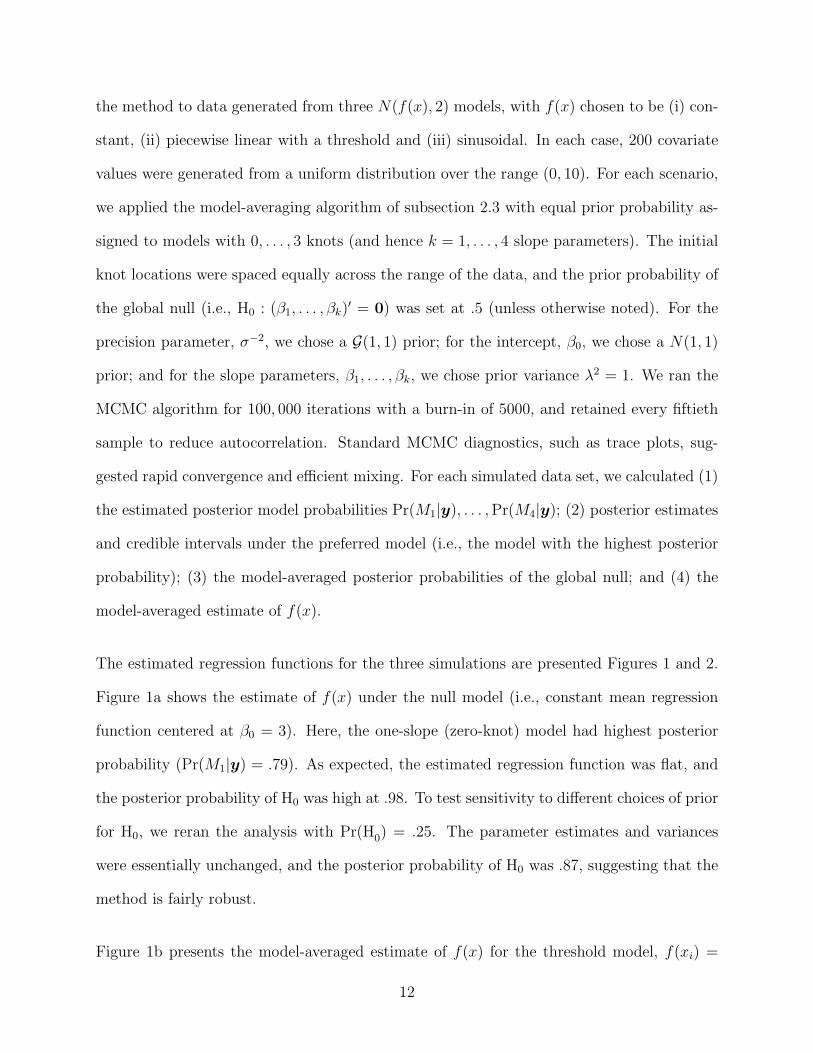
the method to data generated from three N(f(x), 2) models, with f(x) chosen to be (i) con-
stant, (ii) piecewise linear with a threshold and (iii) sinusoidal. In each case, 200 covariate
values were generated from a uniform distribution over the range (0, 10). For each scenario,
we applied the model-averaging algorithm of subsection 2.3 with equal prior probability as-
signed to models with 0, . . . , 3 knots (and hence k = 1, . . . , 4 slope parameters). The initial
knot locations were spaced equally across the range of the data, and the prior probability of
the global null (i.e., H0 : (β1, . . . , βk)′ = 0) was set at .5 (unless otherwise noted). For the
precision parameter, σ−2, we chose a G(1, 1) prior; for the intercept, β0, we chose a N(1, 1)
prior; and for the slope parameters, β1, . . . , βk, we chose prior variance λ2 = 1. We ran the
MCMC algorithm for 100, 000 iterations with a burn-in of 5000, and retained every fiftieth
sample to reduce autocorrelation. Standard MCMC diagnostics, such as trace plots, sug-
gested rapid convergence and efficient mixing. For each simulated data set, we calculated (1)
the estimated posterior model probabilities Pr(M1|y), . . . ,Pr(M4|y); (2) posterior estimates
and credible intervals under the preferred model (i.e., the model with the highest posterior
probability); (3) the model-averaged posterior probabilities of the global null; and (4) the
model-averaged estimate of f(x).
The estimated regression functions for the three simulations are presented Figures 1 and 2.
Figure 1a shows the estimate of f(x) under the null model (i.e., constant mean regression
function centered at β0 = 3). Here, the one-slope (zero-knot) model had highest posterior
probability (Pr(M1|y) = .79). As expected, the estimated regression function was flat, and
the posterior probability of H0 was high at .98. To test sensitivity to different choices of prior
for H0, we reran the analysis with Pr(H0) = .25. The parameter estimates and variances
were essentially unchanged, and the posterior probability of H0 was .87, suggesting that the
method is fairly robust.
Figure 1b presents the model-averaged estimate of f(x) for the threshold model, f(xi) =
12

3 + .5 × I(xi> 8). Our aim here was to determine if the proposed trend test could detect
slight changes in the regression function. For this study, the preferred model had two slope
parameters (Pr(M2|y) = .93). The posterior mean of the single knot, denoted in the graph
by the vertical line, was 8.1. The model-averaged posterior estimate of H0 was .02 (Pr(β1 =
0) = .96 and Pr(β2 = 0) = .02 for the preferred model), suggesting that the method is
powerful enough to detect even a modest threshold effect.
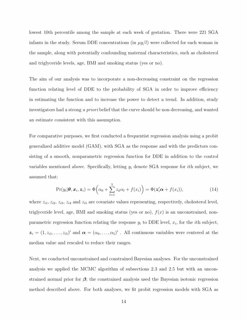
Figure 2 presents results for the sinusoidal mean regression function f(x) = sin(x) + x.
Here, the preferred model had four slopes (Pr(M4|y) = .99). The model-averaged posterior
estimate of H0 was close to 0, as expected. Plotted along with the model-averaged estimate of
f(x) (solid line) in Figure 2 are the true function (dotted line) and a nonparametric estimate
using a typical kernel smoother (dashed line). The results indicate that our approach can
provide a precise estimate of a smooth and highly non-linear regression function. This is
an appealing feature since, as Schell and Singh (1997) point out, traditional approaches
to nonparametric isotonic regression often fit too many knots to the data, resulting in a
uneven estimate of the regression function that is hypersensitive to noise. Because our
procedure uses piecewise linear functions rather than the step functions typically used in
isotonic regression, we can obtain an accurate estimate of the true function with relatively
few knots, thus avoiding an overfit of the data.
4. Application: Effect of DDE on small for gestational age infants
To motivate our approach, we re-analyzed data from a recent study by Longnecker et al.
(2001) examining the effect of DDE exposure on the occurrence of small for gestational
age (SGA) births. DDE is a metabolite of DDT, a pesticide still commonly used in many
developing countries. The sample comprised 2379 pregnant women who were enrolled as
part of the US Collaborative Perinatal Project, a multi-site prospective study of infant
health conducted in the 1960s. Infants were classified as SGA if their birth weight fell in the
13
lowest 10th percentile among the sample at each week of gestation. There were 221 SGA
infants in the study. Serum DDE concentrations (in µg/l) were collected for each woman in
the sample, along with potentially confounding maternal characteristics, such as cholesterol
and triglyceride levels, age, BMI and smoking status (yes or no).
The aim of our analysis was to incorporate a non-decreasing constraint on the regression
function relating level of DDE to the probability of SGA in order to improve efficiency
in estimating the function and to increase the power to detect a trend. In addition, study
investigators had a strong a priori belief that the curve should be non-decreasing, and wanted
an estimate consistent with this assumption.
For comparative purposes, we first conducted a frequentist regression analysis using a probit
generalized additive model (GAM), with SGA as the response and with the predictors con-
sisting of a smooth, nonparametric regression function for DDE in addition to the control
variables mentioned above. Specifically, letting yi denote SGA response for ith subject, we
assumed that:
Pr(yi|θ,xi, zi) = Φ(α0 +
5∑l=1
zilαl + f(xi))
= Φ(z′iα + f(xi)), (14)
where zi1, zi2, zi3, zi4 and zi5 are covariate values representing, respectively, cholesterol level,
triglyceride level, age, BMI and smoking status (yes or no), f(x) is an unconstrained, non-
parametric regression function relating the response yi to DDE level, xi, for the ith subject,
zi = (1, zi1, . . . , zi5)′ and α = (α0, . . . , α5)
′ . All continuous variables were centered at the
median value and rescaled to reduce their ranges.
Next, we conducted unconstrained and constrained Bayesian analyses. For the unconstrained
analysis we applied the MCMC algorithm of subsections 2.3 and 2.5 but with an uncon-
strained normal prior for β; the constrained analysis used the Bayesian isotonic regression
method described above. For both analyses, we fit probit regression models with SGA as
14

response and modelled DDE using four piecewise linear models with k = 1, . . . , 4 slopes,
respectively. For both analyses, we chose a conditionally conjugate N(m0,Σ0) prior for α,
with m0 = (1, 1, 1, 1, 1)′ and Σ0 = diag(10, . . . , 10). Priors for the other model parameters
were similar to those described in Section 3 above. (Sensitivity analysis using different pri-
ors yielded nearly identical results.) We ran the simulations for 100, 000 iterations with a
burn-in of 5000, retaining every fiftieth observation to reduce autocorrelation.
The results are presented in Table 1 and Figure 3. The estimates and standard errors of the
auxiliary parameters, α, were similar under all three models (Table 1), which suggests that
our proposed approach does not induce bias. Figure 3 plots the estimated risk difference
across DDE exposure for the reference group under the various models. The y-axis shows
the change in probability of SGA compared to minimum exposure. Figure 3(a) presents
the risk difference for both the unconstrained GAM and unconstrained Bayesian models.
The GAM model indicated a significant overall effect for DDE (p=.02, 2.9 nonparametric
df). For both analyses, however, the effect was highly nonlinear, with a modest positive
effect for low to moderate exposures and a strong negative effect for very high exposures.
This somewhat counterintuitive finding is due, in part, to the relatively few subjects with
very high exposures, most of whom were SGA negative. In absence of the monotonicity
constraint, these subjects exert a strong influence on the regression function f(x) in these
models. Incidentally, these SGA negative women with high exposures do not invalidate the
monotonicity assumption. Few would argue, for example, that DDE is less detrimental at
higher exposures. Rather, in this sample, there appear to be some women who were resistant
to the effect of DDE, even at high doses. It is possible that women who were susceptible to
high DDE exposures had fetal loss rather than SGA-positive deliveries (Longnecker et al.,
2003), and hence only SGA-negative pregnancies were reported at these extreme exposures.
Figure 3(b) presents the estimated risk difference and 95% credible intervals under the pro-
15

posed constrained Bayesian approach. For this analysis, the preferred model had two slope
parameters (one knot), with a posterior model probability Pr(M2|y) = .76, followed by the
model with only one slope parameter (Pr(M1|y) = .22). The model-averaged posterior prob-
ability of the global null was .04, indicating strong evidence of a trend. In particular, there
appears to be a 5% increase in the effect of DDE for low exposure levels, with the effect
tapering off after a threshold of about 20 µg/l. The figure also shows larger variance at
high exposure levels. Again, this is due to the relatively few subjects in this range, most of
whom were SGA negative. Nevertheless, the posterior variance for the constrained regression
function was 44% lower than that for the unconstrained regression function, suggesting an
improvement in efficiency.
5. Discussion
This article has proposed a practical Bayesian approach for order restricted inference on
continuous regression functions in generalized linear models. This approach has several
distinct advantages. First, monotonicity constraints can be incorporated for a wide class of
models, resulting in improved efficiency and increased power to detect effects. Second, flat
regions in the regression curve (i.e., regions of no effect) are easily accommodated and can
be used as a basis for trend testing. Third, the analyst can specify the prior probability
of the global null and can conduct multiple hypothesis tests over subregions of the data
in way that controls the Type-I error rate. As the simulations demonstrated, a smooth
but accurate estimate of the regression curve can be obtained with relatively few knots.
Moreover, knot locations are data driven, rather than arbitrarily chosen. And finally, a
simple model-averaging approach can be used to account for uncertainty in the number of
knots.
As illustrated through the DDE application, the proposed method also enables one to ac-
16

curately estimate thresholds, a feature that should find wide appeal among toxicologists,
environmental epidemiologists and other researchers concerned with threshold estimation.
The results from simulation studies also suggest that the procedure is robust to different
prior specifications and to number of knots chosen. The approach can easily be generalized
to handle more complex models, such as random effect and survival models. One can also
extend the procedure to accommodate more complex ordering structures, such as umbrella
orderings, by allowing the peak to occur at a knot having an unknown location and extending
the MCMC algorithm appropriately.
ACKNOWLEDGEMENTS
The authors would like to thank Zhen Chen and Sean O’Brien for helpful comments and
discussions. Thanks also to Matthew Longnecker for providing the data for the example.
17

Appendix A: Full Conditional for βj
The form of the full conditional for βj(j = 1, . . . , k) depends on the value of βj+1, for
j = 1, . . . , k − 1. In the simple case, where βj+1 = 0, for j = 2, . . . , k − 1, we have:
π(βj|β(−j), βj+1 = 0,γ, σ2,y) = ZI-N+(βj; π(1)j , E
(1)j , V
(1)j ), (15)
where E(1)j = V
(1)j
(σ−2
n∑i=1
wijy∗i +λ−2βj−1
), V
(1)j =
(σ−2
n∑i=1
w2ij+λ
−2
)−1
, y∗i = yi−k∑
l: l 6=jwilβl,
and π(1)j =
π0jΦ(βj−1/λ)N(0;E(1)j ,V
(1)j )
π0jΦ(βj−1/λ)N(0;E(1)j ,V
(1)j )+(1−π0j)Φ
(E
(1)j /
√V
(1)j
)N(βj−1;0 , λ2)
.
In the case where βj+1 > 0 for j = 2, . . . , k − 1, we instead have:
π(βj|β(−j), βj+1 > 0,γ, σ2,y) = π(2)j 1(βj=0) + (1− π
(2)j )
N(βj;E(2)j , V
(2)j )1(βj>0)
Φ(βj/λ)∫∞0
N(βj ;E(2)j ,V
(2)j )
Φ(βj/λ)dβj
, (16)
where E(2)j = V
(2)j
(σ−2
n∑i=1
wijy∗i + λ−2(βj−1 + βj+1)
), V
(2)j =
(σ−2
n∑i=1
w2ij + 2λ−2
)−1
,
and π(2)j =
2π0jΦ(βj−1/λ)N(0;E(2)j ,V
(2)j )
2π0jΦ(βj−1/λ)N(0;E(2)j ,V
(2)j )+(1−π0j)N(βj−1;0 , λ2)
∫∞0
N(βj ;E(2)j
,V(2)j
)
Φ(βj/λ)dβj
.
For j = 1, the full conditional distribution follows the same form, but with βj−1 set equal
to 0. For j = k, the form is as shown in expression (15). The MCMC algorithm proceeds
by sampling βj directly from its full conditional (15) if β(0)j+1 = 0 or if j = k. If j < k
and β(0)j+1 > 0, draw a value from the full conditional (16) by using the following sampling
importance-resampling procedure:
1. Draw δj Bernoulli(π(2)j ) where π
(2)j =
∫∞0
N(βj ;E(2)j ,V
(2)j )
Φ(βj/λ)dβj (obtained numerically);
2. If δj = 1, set βj = 0 and otherwise draw r values βj1, . . . , βjr fromN(βj;E(2)j , V
(2)j )1(βj>0),
and then choose one of these values by sampling from βj1, . . . , βjr with probabilities
Φ(βj1/λ)−1, . . . ,Φ(βjr/λ)−1. For our analyses, we chose r = 100.
18
REFERENCES
Albert, J.H. and Chib, S. (1993). Bayesian analysis of binary and polychotomous response
data. Journal of the American Statistical Association, 88, 669-679.
Chen, M.-H. and Shao, Q.-M. (1998). Monte Carlo methods on Bayesian analysis of con-
strained parameter problems. Biometrika 85, 73-87.
Chen, M.-H., Shao, Q.-M. and Ibrahim, J.G. (2000). Monte Carlo Methods in Bayesian
Computation. New York: Springer.
Chipman, H., George, E.I., and McCulloch, R.E. (2001). The practical implementation of
Bayesian model selection. IMS Lecture Notes - Monograph Series 38.
Dunson, D.B. and Neelon, B. (2003). Bayesian inferences on order constrained parameters
in generalized linear models. Biometrics 59, 286-295.
Gelfand, A.E. and Kuo, L. (1991). Nonparametric Bayesian bioassay including ordered
polytomous response. Biometrika 78, 657-666.
Gelfand, A.E. and Smith, A.F.M. (1990) Sampling based approaches to calculating marginal
densities. Journal of the American Statistical Association 85, 398-409.
Gelfand, A.E., Smith, A.F.M., and Lee, T.M. (1992). Bayesian analysis of constrained pa-
rameter and truncated data problems using Gibbs sampling. Journal of the American
Statistical Assocation 87, 523-532.
George, E.I. and McCulloch, R.E. (1997). Approaches for Bayesian variable selection.
Statistica Sinica 7, 339-373.
Gilks, W.R. and Wild, P. (1992). Adaptive rejection sampling for Gibbs sampling. Applied
Statistics 41, 337-348.
19

Geweke, J. (1996). Variable selection and model comparison in regression. In Bayesian
Statistics 5, J.O. Berger, J.M. Bernardo, A.P. Dawid, and A.F.M. Smith (eds.). Oxford
University Press, 609-620.
Green, P.J. (1995). Reversible jump Markov chain Monte Carlo computation and Bayesian
model determination, Biometrika, 82, 711-732.
Hastie, T.J. and Tibshirani, R.J. (1990). Generalized Additive Models. London: Chapman
& Hall.
Hastings, W.K. (1970). Monte Carlo sampling methods using Markov chains and their
applications. Biometrika 57, 97-109.
Holmes, C.C. and Heard, N.A. (2003). Generalised monotonic regression using random
change points. A revised version has appeared in Statistics in Medicine 22, 623-638.
Holmes, C.C. and Mallick, B.M. (2001). Bayesian regression with multivariate linear splines.
Journal of the Royal Statistical Society, Series B 63, 3-17.
Johnson, N.L. and Kotz, S. (1970). Continuous Univariate Distributions - I. Distributions
in Statistics. New York: John Wiley & Sons.
Lavine, M. and Mockus, A. (1995). A nonparametric Bayes method for isotonic regression.
Journal of Statistical Planning and Inference 46, 235-248.
Lognecker, M.P., Klebanoff, M.A., Zhou, H. and Brock, J.W. (2001). Association between
maternal serum concentration of the DDT metabolite DDE and preterm and small-for
gestational-age babies at birth. The Lancet 258, 110-114.
Longnecker M.P., Klebanoff M.A., Dunson D.B., Guo X., Chen Z., Zhou H., Brock J.W.
(2003). Maternal serum level of the DDT metabolite DDE in relation to fetal loss in
previous pregnancies. Environmental Research. In press.
20
Mengersen, K.L. and Tweedie, R.L. (1996). Rates of convergence of the Hastings and
Metropolis algorithms. Annals of Statistics 24, 101-121.
Molitor, J. and Sun, D.C. (2002). Bayesian analysis under ordered functions of parameters.
Environmental and Ecological Statistics 9, 179-193.
Raftery, A.E. (1996). Approximate Bayes factors for accounting for model uncertainty in
generalised linear models. Biometrika 83, 251-266.
Raftery, A.E., Madigan, D., and Hoeting, J.A. (1997). Bayesian model averaging for linear
regression models. Journal of the American Statistical Association 92, 179-191.
Ramgopal, P., Laud, P.W. and Smith, A.F.M. (1993). Nonparametric Bayesian bioassay
with prior constraints on the shape of the potency curve. Biometrika 80, 489-498.
Robertson, T., Wright, F. and Dykstra, R. (1988) Order Restricted Statistical Inference.
New York: Wiley.
Schell, M. and Singh, B. (1997). The reduced monotonic regression method. Journal of the
American Statistical Association 92, 128-135.
Tierney, L. (1994) Markov chains for exploring posterior distributions. Annals of Statistics
22, 1701-1762.
Westfall P.H., Johnson W.O., Utts J.M. (1997). A Bayesian perspective on the Bonferroni
adjustment. Biometrika 84 419-427.
21

Table 1
Estimates of control variable regression coefficients for the DDE Analysis.
Description Parameter GAM† (sd) Constrained‡ Unconstrained?
Mean (sd) Mean (sd)
Intercept α0 -1.5 (.42) -2.2(.44) -1.87 (.41)Cholesterol α1 -.13 (.06) -.12 (.006) -.13(.06)
Triglycerides α2 -.13 (.05) -.13(.06) -.13 (.05)Age α3 .01 (.006) .01 (.006) .01 (.006)BMI α4 -.26 (.10) -.28 (.10) -.27(.10)
Smoking Status α5 .38 (.08) .38 (.07) .39 (.08)
† Results using frequentist GAM with nonparametric function for DDE.
‡ Analysis using approach described here with one random knot (preferred model).
? Unconstrained Bayesian analysis with one random knot.
22

Figure 1. Model-averaged estimated posterior regression functions for a) the
null model f(x) = 3 and b) the threshold model f(x) = 3 + .5 × I(x>8).
The dotted lines represent 95% credible intervals. The vertical line in Fig-
ure (b) denotes the posterior mean of knot γ for the preferred model.
••
•
•
•
•
•
••
•••
• •
•
••
•
•
•
•
• ••
•
•
•••
•••
•
•
• •
• ••
•
••
••
•
•
•
••
••
•
•
•
•
•
•
•
•• • •
•
•
••
•••
•••
•
•
•
•
•
• •
•••
•
•
• •
•
••
•
•
•
•
•
•
•
••
•
•
••
•
•
••
•
•
•
•
•
••
••
•
•
•
••
••
•
•
•
•
•
••
•• ••
••
•
••
•
•
••
•
•
•• •
•
•
••
•
•
•
••
••
•
•••
••
•
•
• ••• ••
••
•
•
•
•••
•
•
• •••••
•
•
••
•
••
•• • • •
x
y
0 2 4 6 8 10
02
46
pr(H0 | y) =.98
a
••
•
•
•
•
•
•
•
••
•
• •
•
••
•
•
•
•
• •
•
•
•
•••
•••
•
•
• •
••
•
•
•
•
••
•
•
•
•
••••
•
•
•
•
•
•
•• • •
•
•
• •
•••
• •••
•
•
•
•
• •
•
••
•
•
••
•
••
•
•
•
•
•
•
•
•
••
•
•
•
•
•
••
•
•
•
•
•
•
••
•
•
•
•
••
••
•
•
•
•
•
••
•• •
•
••
•
••
•
•
••
•
•
•• •
•
•
••
•
•
••
•
•
••
•
••
••
•
•
• ••• ••
••
••
•
•••
•
•
• •••••
•
•
••
•
•
••• • • •
x
y
0 2 4 6 8 10
02
46
b
pr(H0 | y) =.03
23

Figure 2. Model-averaged estimated posterior regression function for f(x) = sin(x) + x.
The solid line is from a Bayesian isotonic regression analysis, the dotted line is the
true regression function, and the dashed line is from a typical kernel smoother. Ver-
tical lines denote the posterior means of the interior knots for the preferred model.
•
•
•
•
••
• •
••
• •
•
•
••
••
•
••
••
•
••
•
•
•
•
•
• •
•
•
•
•
•
•
•
•
•
•
•
•
•
•
•
•
•
••
•
•
•
•
•
•
••
• •
•
•
•
••
•
•
•
•
•
•
•
•
•
••
•
•
•
•
•
•
••
•
•
• •
••
•
•
•
•
•
•••
•
•
•
•
•
••••
•
•
•
•
•
•
•
•
•
•
••
•
•
••
•
•
•
••
•
•
•
•
•
•
••
•
••
•
•
••
•
•
•
•
•
•
•
•
•
•
•
•
••
•
•
•
•
•
•
• •
•
• •
•
•
•
•
•
•
•
•
•
•
•
•
•
••
••
•
•
•
• ••
•
•
•
••
•
•
x
y
0 2 4 6 8 10
-20
24
68
1012 pr(H0 | y) = 0 PWL
True Fn Kernel
24

Figure 3. Estimated risk difference plots for (a) the unconstrained GAM and Bayesian
analyses and (b) the constrained Bayesian analysis. The vertical lines denote the
posterior means of the interior knots for the preferred (a) unconstrained and (b) con-
strained Bayesian models. Dotted lines in Figure (b) represent 95% credible intervals.
Serum DDE (micro g/L)
Ris
k D
iff
0 20 40 60 80 100 120 140 160 180-0.05
0.0
0.05
0.10
0.15
0.20
(a)
Unconstrained Bayes Unconstrained GAM
Serum DDE (micro g/L)
Ris
k D
iff
0 20 40 60 80 100 120 140 160 180-0.05
0.0
0.05
0.10
0.15
0.20
(b)
pr(H0 | y) =.04
25