Bayesian Inference under Differential Privacy

Bayesian Inference under Differential Privacy

Yonghui XiaoEmory UniversityAtlanta, GA, USA

[email protected]

Li XiongEmory UniversityAtlanta, GA, USA

[email protected]

ABSTRACTBayesian inference is an important technique throughoutstatistics. The essence of Beyesian inference is to derivethe posterior belief updated from prior belief by the learnedinformation, which is a set of differentially private answersunder differential privacy. Although Bayesian inference canbe used in a variety of applications, it becomes theoreticallyhard to solve when the number of differentially private an-swers is large. To facilitate Bayesian inference under differ-ential privacy, this paper proposes a systematic mechanism.The key step of the mechanism is the implementation ofBayesian updating with the best linear unbiased estimatorderived by Gauss-Markov theorem. In addition, we also ap-ply the proposed inference mechanism into an online query-answering system, the novelty of which is that the utilityfor users is guaranteed by Bayesian inference in the form ofcredible interval and confidence level. Theoretical and ex-perimental analysis are shown to demonstrate the efficiencyand effectiveness of both inference mechanism and onlinequery-answering system.

1. INTRODUCTIONData privacy issues frequently and increasingly arise for

data sharing and data analysis tasks. Among all the privacy-preserving mechanisms, differential privacy has been widelyaccepted for its strong privacy guarantee [8, 9]. It requiresthat the outcome of any computations or queries is formallyindistinguishable when run with and without any particularrecord in the dataset. To achieve differential privacy theanswer of a query is perturbed by a random noise whosemagnitude is determined by a parameter, privacy budget.

Existing mechanisms[10, 7, 2, 20] of differential privacyonly has a certain bound of privacy budget to spend onall queries. We define the privacy bound as overall pri-vacy budget and such system bounded differentiallyprivate system. To answer a query, the mechanism al-locates some privacy budget(also called privacy cost of thequery) for it. Once the overall privacy budget is exhausted,

either the database has to be shut down or any further querywould be rejected. To prevent budget depletion and extendthe lifetime of such systems, users have the burden to al-locate privacy budget for the system. However, there is notheoretical clue on how to allocate budget so far.

To save privacy budget, existing work uses the correlatedanswers to make inference about new-coming queries. Cur-rent literature falls into one of the following: 1. Query ori-ented strategy. Given a set of queries(or answers) and thebound of privacy budget, optimize answers according to thecorrelation of queries[18, 4, 5]; 2. Data oriented strategy.Given the privacy bound, maximize the global utility of re-leased data[13, 26, 27]; 3. Inference oriented strategy.Use traditional inference method, like MLE, to achieve aninference result or bound[23, 24, 17]. All existing work canonly make point estimation, which provides limited useful-ness due to lack of probability properties. Some work givesan error tolerance of the inference, like [ε, δ]-usefulness[3].However, Bayesian inference has not been achieved yet.

Bayesian inference is an important technique throughoutstatistics. The essence of Beyesian inference is to derive theposterior belief updated from prior belief by the learned in-formation, which is a set of differentially private answers inthis paper. With Bayesian inference, a variety of applica-tions can be tackled. Some examples are shown as follows.

• hypothesis testing. If a user(or an attacker) makes ahypothesis that Alice’s income is higher than 50 thou-sand dollars, given a set of Alice’s noisy income 1 ,what is the probability that the hypothesis holds?

• credible interval and confidence level. If a userrequires an interval in which the true answer lies withconfidence level 95%, how can we derive such an inter-val satisfying the requirement?

Other applications, like regression analysis, statistical in-ference control and statistical decision making, can also befacilitated by Bayesian inference.

Although having so many applications, Bayesian inferencebecomes theoretically hard to solve when the number of dif-ferentially private answers, denoted as “history” queries, islarge. This phenomenon is often referred as the curse of highdimensionality if we treat each answer in “history” as an in-dependent dimension. Because the derivation of posteriorbelief involves a series of integrals of probability function 2 ,

1It complies with the assumption of differential privacy thatan adversary knows the income of all other people but Alice.2For convenience and clearance, probability function onlyhas two meanings in this paper: probability density function

arX

iv:1

203.

0617

v2 [

cs.D

B]

9 N

ov 2

012

we show later in this paper the complexity of the probabilityfunction although it can be processed in a closed form3.

Contributions. This paper proposes a systematic mech-anism to achieve Bayesian inference under differential pri-vacy. Current query-answering mechanisms, like Laplacemechanism[10] and exponential mechanism[21], have alsobeen incorporated in our approach. According to thesemechanisms, a set of “history” queries and answers witharbitrary noises can be given in advance. The key step ofour mechanism is the implementation of Bayesian updatingabout a new-coming query using the set of “history” queriesand answers. In our setting, uninformative prior belief isused, meaning we do not assume any evidential prior beliefabout the new query. At first, a BLUE(Best Linear Un-biased Estimator) can be derived using Gauss-Markov the-orem or Generalized Least Square method. Then we pro-pose two methods, Monte Carlo(MC) method and Proba-bility Calculation(PC) method, to approximate the proba-bility function. At last, the posterior belief can be derivedby updating the prior belief using the probability function.Theoretical and experimental analysis have been given toshow the efficiency and accuracy of two methods.

The proposed inference mechanism are also applied in anonline utility driven query-answering system. First, it canhelp users specify the privacy budget by letting users de-mand the utility requirement in the form of credible intervaland confidence level. The key idea is to derive the credibleinterval and confidence level from the history queries usingBayesian inference. If the derived answer satisfies user’s re-quirement, then no budget needs to be allocated because theestimation can be returned. Only when the estimation cannot meet the utility requirement, the query mechanism isinvoked for a differentially private answer. In this way, notonly the utility is guaranteed for users, but also the privacybudget can be saved so that the lifetime of the system canbe extended. Second, We further save privacy budget by al-locating the only necessary budget calculated by the utilityrequirement to a query. Third, the overall privacy cost ofa system is also measured to determine whether the systemcan answer future queries or not. Experimental evaluationhas been shown to demonstrate the utility and efficiency.

All the algorithms are implemented in MATLAB, and allthe functions’ names are consistent with MATLAB.

2. PRELIMINARIES AND DEFINITIONSWe use bold characters to denote vector or matrix, normal

character to denote one row of the vector or matrix; sub-script i, j to denote the ith row, jth column of the vector ormatrix; operator [·] to denote an element of a vector; θ, θ todenote the true answer and estimated answer respectively;AQ to denote the differentially private answer of Laplacemechanism.

2.1 Differential privacy and Laplace mecha-nism

for continuous variables and probability mass function fordiscrete variables.3A closed form expression can be defined by a finite numberof elementary functions(exponential, logarithm, constant,and nth root functions) under operators +,−,×,÷.

Definition 2.1 (α-Differential privacy [7]). A dataaccess mechanism A satisfies α-differential privacy4 if forany neighboring databasesD1 and D2, for any query func-tion Q, r ⊆ Range(Q)5, AQ(D) is the mechanism to returnan answer to query Q(D),

supr⊆Range(Q)

Pr(AQ(D) = r|D = D1)

Pr(AQ(D) = r|D = D2)≤ eα (1)

α is also called privacy budget.

Note that it’s implicit in the definition that the privacy pa-rameter α can be made public.

Definition 2.2 (Sensitivity). For arbitrary neighbor-ing databases D1 and D2, the sensitivity of a query Q is themaximum difference between the query results of D1 and D2,

SQ = max|Q(D1)−Q(D2)|

For example, if one is interested in the population size of0 ∼ 30 old, then we can pose this query:

• Q1: select count(*) from data where 0 ≤ age ≤ 30

Q1 has sensitivity 1 because any change of 1 record can onlyaffect the result by 1 at most.

Definition 2.3 (Laplace mechanism). Laplace mech-anism[10] is such a data access mechanism that given a user

query Q whose true answer is θ, the returned answer θ is

AQ(D) = θ + N(α/S) (2)

N(α/S) is a random noise of Laplace distribution. If S = 1,the noise distribution is like equation (3).

f(x, α) =α

2exp(−α|x|); (3)

For S 6= 1, replace α with α/S in equation (3).

Theorem 2.1 ([10, 7]). Laplace mechanism achieves α-

differential privacy, meaning that adding N(α/SQ) to Q(D)guarantees α-differential privacy.

2.2 UtilityFor a given query Q, denote θ the true answer of Q.

By some inference methods, a point estimation θ can beobtained by some metrics, like Mean Square Error(MSE)

E[(θ − θ)2]. Different from point estimation, interval esti-mation specifies instead a range within which the answerlies. We introduce (ε, δ)-usefulness[3] first, then show thatit’s actually a special case of credible interval, which will beused in this paper.

Definition 2.4 ((ε, δ)-usefulness [3]). A query answer-

ing mechanism is (ε, δ)-useful for query Q if Pr(|θ − θ| ≤ε) ≥ 1− δ.

Definition 2.5 (credible interval[12]). Credible in-terval with confidence level 1 − δ is a range [L,U ] with theproperty:

Pr(L ≤ θ ≤ U) ≥ 1− δ (4)

4Our definition is consistent with the unbounded modelin[15].5Range(Q) is the domain of the differentially private answerof Q.

In this paper, we let 2ε = U − L to denote the length ofcredible interval. Note when θ is the midpoint of L(Θ) and

U(Θ), these two definitions are the same and have equal ε.Thus (ε, δ)-usefulness is a special case of credible interval.An advantage of credible interval is that users can specifycertain intervals to calculate confidence level. For example,a user may be interested in the probability that θ is largerthan 10.

In our online system, the utility requirement is the 1 − δcredible interval whose parameter δ is specified by a userto demand the confidence level of returned answer. Intu-itively, the narrower the interval, the more useful the answer.Therefore, we also let users specify the parameter ε so thatthe length of interval can not be larger than 2ε, U −L ≤ 2ε.

2.3 Bayesian UpdatingThe essence of Beyesian inference is to update the prior

belief by the learned information(observations), which is ac-tually a set of differentially private answers in this paper.Assume a set of observations is given as θ1, θ2, · · · , θn. Instep i, denoted fi−1(θ) the prior belief of θ, which can be

updated using the observation θi by Bayes’ law as follows:

fi(θ) = fi−1(θ)Pr(θi = θ|θ)Pr(θi)

(5)

where fi(θ) is the posterior belief at step i. It is also theprior belief at step i+ 1.

Above equation justifies why we use uninformative priorbelief(also called a priori probability[12] in some literature)as the original prior belief because any informative(evidential)prior belief can be updated from uninformative belief. It isthe same we take either the informative prior belief or theposterior belief updated from uninformative prior belief asthe prior belief.

2.4 Data model and example

2.4.1 DataConsider a dataset withN nominal or discretized attributes,

we use anN -dimensional data cube, also called a base cuboidin the data warehousing literature [19, 6], to represent theaggregate information of the data set. The records are thepoints in the N -dimensional data space. Each cell of adata cube represents an aggregated measure, in our case,the count of the data points corresponding to the multidi-mensional coordinates of the cell. We denote the numberof cells by n and n = |dom(A1)| ∗ · · · ∗ |dom(AN )| where|dom(Ai)| is the domain size of attribute Ai.

xx

Income

ID Age Income x2x1

2010

>50K

ID Age Income1 0~30 0~50K

x3 x4

20 10

0~50

2 0~30 >50K

… … …20 10

0~30 >30

K

60 >30 >50K

Ageg

Figure 1: Example original data represented in a rela-

tional table (left) and a 2-dimensional count cube (right)

• Example. Figure 1 shows an example relational datasetwith attribute age and income (left) and a two-dimensionalcount data cube or histogram (right). The domain val-ues of age are 0∼30 and > 30; the domain values ofincome are 0∼50K and > 50K. Each cell in the datacube represents the population count corresponding tothe age and income values. We can represent the orig-inal data cube, e.g. the counts of all cells, by an n-dimensional column vector x shown below.

x =[

10 20 20 10]T

(6)

2.4.2 QueryWe consider linear queries that compute a linear combi-

nation of the count values in the data cube based on a querypredicate.

Definition 2.6 (Linear query [18]). A set of linearqueries Q can be represented as an q×n-dimensional matrixQ = [Q1; . . . ;Qq] with each Qi is a coefficient vector of x.The answer to Qi on data vector x is the product Qix =Qi1x1 + Qi2x2 + · · ·+ Qinxn.

• Example. If we know people with income ≤ 50Kdon’t pay tax, people with income > 50K pay 2Kdollars, and from the total tax revenue 10K dollars areinvested for education each year, then to calculate thetotal tax, following query Q2 can be issued.

– Q2: select 2∗count() where income > 50 − 10

Q2 = [ 2 2 0 0 ] (7)

AQ2 = Q2 · x + N(α/SQ2) (8)

Q2 has sensitivity 2 because any change of 1 record canaffect the result by 2 at most. Note that the constant10 does not affect the sensitivity of Q2 because it won’tvary for any record change 6. Equation (7) shows thequery vector of Q2. The returned answer AQ2 fromLaplace mechanism are shown in equation (8) where αis the privacy cost of Q2.

Given a m × n query “history” H, the query answer forH is a length-m column vector of query results, which canbe computed as the matrix product Hx.

2.4.3 Query history and Laplace mechanismFor different queries, sensitivity of each query vector may

not be necessarily the same. Therefore, we need to computethe sensitivity of each query by Lemma 2.1.

Lemma 2.1. For a linear query Q, the sensitivity SQ ismax(abs(Q)).

where function “abs()” to denote the absolute value of avector or matrix, meaning that for all j, [abs(Q)]j = |Qj |.max(abs(Q)) means the maximal value of abs(Q).

We can write the above equations in matrix form. Lety, H, α and S be the matrix form of AQ, Q, α and S re-spectively. According to Lemma 2.1, S = maxrow(abs(H))where maxrow(abs(H)) is a column vector whose items arethe maximal values of each row in abs(H).

6So we ignore any constants in Q in this paper.

Equations(9, 10) summarize the relationship of y, H, x,

N and α.

y = Hx + N(α./S) (9)

S = maxrow(abs(H)) (10)

where operator ./ means ∀i, [α./S]i = αi/Si.

• Example. Suppose we have a query history matrix Has equation (11), x as equation (6) and the privacy pa-rameter A used in all query vector shown in equation(12).

H =

1 1 0 00 0 1 10 0 0 10 0 1 00 1 0 12 1 0 00 0 2 -10 -1 0 1

(11)

α =[

.05 .1 .05 .1 .1 .05 .05 .1]T (12)

Then according to Lemma 2.1, S can be derived inequation (13).

S =[

1 1 1 1 1 2 2 1]T

(13)

Therefore, the relationship of y, H, A and S in equa-tion (9) can be illustrated in equation (14)

y1y2y3y4y5y6y7y8

=

1 1 0 00 0 1 10 0 0 10 0 1 00 1 0 12 1 0 00 0 2 -10 -1 0 1

x + N

0.05/10.1/10.05/10.1/10.1/10.05/20.05/20.1/1

(14)

3. THE BEST LINEAR UNBIASED ESTI-MATOR

Given a set of target queries as Q and equations (9,10), theBLUE can be derived in the following equation by Gauss-Markov theorem or Generalized Least Square method sothat MSE(x) can be minimized.

x = (HT diag2(α./S)H)−1HT diag2(α./S)y (15)

where function diag() transforms a vector to a matrix witheach of element in diagonal; diag2() = diag() ∗ diag(). Forestimatability, we assume rank(H) = n. Otherwise x maynot be estimable 7.

Theorem 3.1. To estimate Θ = Qx, which is a q × 1query vector, Q ∈ Rq×n, the linear estimator Θ = Ayachieves minimal MSE when

A = Q(HT diag2(α./S)H)−1HT diag2(α./S) (16)

In the rest of the paper, we will focus on a query. Thuswe assume Q ∈ R1×n and θ = Qx. However, this work canbe easily extended to multivariate case using multivariateLaplace distribution[11].

7However, Θ = Qx may also be estimable iff Q =Q(HTH)−HTH where (HTH)− is the generalized inverseof HTH.

Corollary 3.1. θ is unbiased, meaning E(θ) = θ.

Corollary 3.2. The mean square error of θ equals tovariance of θ,

MSE(θ) = Var(θ) = 2Q(HT diag2(α./S)H)−1QT (17)

A quick conclusion about (ε, δ)-usefulness can be drawnusing Chebysheve’s inequality.

Theorem 3.2. The (ε, δ)-usefulness for θ is satisfied when

δ = V ar(θ)

ε2, which means

Pr(|θ − θ| ≤ ε) ≥ 1− V ar(θ)

ε2(18)

However, the above theorem only gives the bound of δinstead of the probability Pr(|Θi − Θi| ≤ ε) which can bederived by Bayesian inference.

• Example. Let Q =[

1 0 1 0], y = [30.8, 30.3, 46.9,

20.2, 30.4, 68.9, 38.9, 9.5]T . First, we can derivediag(α./S) as

diag(α./S) =

.05 0 0 0 0 0 0 00 .1 0 0 0 0 0 00 0 .05 0 0 0 0 00 0 0 .1 0 0 0 00 0 0 0 .1 0 0 00 0 0 0 0 .025 0 00 0 0 0 0 0 .025 00 0 0 0 0 0 0 .1

Then by Theorem 3.1, we have x = [24.9, 10.1, 17.0, 19.5]T ,

θ = 42.0.

4. BAYESIAN INFERENCEIn equation (5), Bayesian inference involves three major

components: prior belief, observation(s) and the conditional

probability Pr(θi|θ). Then from last section, an estimator

θ = Ay can be obtained. We take uninformative prior belief,meaning we do not assume any evidential prior belief aboutθ. Because Pr(θi) can be calculated as

∫f(θi|θ)fi−1(θ)dθ,

the remaining question is to calculate the conditional prob-ability Pr(θi = θ|θ).

We denote fZ(z) a probability function of Z, fZ(x) a prob-ability function of Z with input variable x. For example, iffN (x) is the probability function of N whose probabilityfunction is shown in equation (3), following equation showsfN (z).

fN (z) =α

2exp(−α|z|); (19)

Then Pr(θi = θ|θ) = fθ(z)|θ=z.

4.1 Theoretical Probability FunctionLemma 4.1. The probability function of fθ(θ) is the prob-

ability function of fAN(Ay− θ).

Proof.

θ = Ay = A(Hx + N) = Qx + AN = θ + AN

=⇒ θ = Ay−AN

=⇒ Pr(θ = θ) = Pr[AN = Ay− θ]

Because of the above equation, we have

fθ(θ) = fAN(Ay− θ)

Theorem 4.1. The probability function of θ is

fθ(θ) =1

2π

∫ ∞−∞

exp(−it(Ay− θ))m∏k=1

α2k

α2k + (A2

kS2k)t2

dt

(20)

Proof. The noise for a query with sensitivity Si is Lap(αi/Si).It’s easy to compute the characteristic function of Laplacedistribution is

ΦNi(t) =

α2i

S2i t2 + α2

i

(21)

AN =∑mk=1 AkNk, so the characteristic function of AN is

ΦAN =

m∏k=1

α2k

S2kA

2kt

2 + α2i

(22)

Then the probability function of AN is

fAN(θ) =1

2π

∫ ∞−∞

exp(−itθ)m∏k=1

α2k

α2k + (A2

kS2k)t2

dt

Therefore, by Lemma 4.1, we have equation (20).

The probability function can also be represented in a closedform using multivariate Laplace distribution in [11]. It hasalso been proven in [11] that linear combination of Laplacedistribution is also multivariate Laplace distributed. To re-duce the complexity, the probability function of sum of nidentical independent distributed Laplace noises can be de-rived as follows[14].

fn(z) =αn

2nΓ2(n)exp(−α|z|)

∫ ∞0

vn−1(|z|+v

2α)n−1e−vdv

(23)

We can see that even the above simplified equation be-comes theoretically hard to use when n is large. More prob-ability functions can be found in [16].

To circumvent the theoretical difficulty, two algorithms,Monte Carlo(MC) and discrete probability calculation(PC)method, are proposed to approximate the probability func-tion. Error of the approximation is defined to measure theaccuracy of the two algorithms. By comparing the errorand computational complexity, we discuss that both of themhave advantages and disadvantages.

4.2 Monte Carlo Probability FunctionWe show the algorithm to derive Monte Carlo probabil-

ity as follows. It uses sampling technique to draw randomvariables from a certain probability function. We skip de-tailed sampling technique, which can be found in literatureof statistics, like [12, 1, 16].

Algorithm 1 Derive the probability function of θ by MonteCarlo methodRequire: ms: sample size for a random variable; α: pri-

vacy budget; S: sensitivity; A: θ = Ay; m: H ∈ Rm×n1. Y = 0, which is a ms × 1 vector;for k = 1; k < m; k + + do

Draw ms random variables from distributionLap(αk/Sk); denote the variables as Xk;multiply Ak to Xk, denote as AkXk;Y = Y + AkXk;

end for2. Y = round(Y).3. Plot the histogram of Y:

3.1 |u| = 2 ∗max(abs(Y)) + 1.

3.2 u = hist(Y,− |u|−12

: 1 : |u|−12

)/ms.return The probability mass vector u

The function round(Y) rounds the elements of Y to thenearest integers. The purpose of step 3 is to to guarantee

|u| is an odd number. In step 4, function hist(Y,− |u|−12

:

1 : |u|−12

) returns a vector of number representing the fre-

quency of the vector − |u|−12

: 1 : |u|−12

. For example,

u[1] =∑msi=1 b(Yi = − |u|−1

2)/ms; u[i] =

∑msi=1 b(Yi =

− |u|−12

+ i)/ms where i ∈ Z and b() is a bool function thatreturns 1 as true, 0 as false.

The returned vector u is a probability mass function in adiscretized domain. Following definition explains a proba-bility mass vector v.

Definition 4.1. a probability mass vector vz is the prob-ability mass function of z so that

vi =

∫ i− |v|2

i− |v|2−1

fz(z)dz = Fz(i−|v|2

)− Fz(i−|v|2− 1)

where |v| is the length of v, fz(z) is the probability densityfunction of z, Fz() is the cumulative distribution function.

Note that |v| should be an odd number implicitly to guar-antee the symmetry of probability mass vector.

For example, if v = [0.3, 0.4, 0.3], it means v1 =∫ −0.5

−1.5fz(z)dz =

0.3, v2 =∫ 0.5

−0.5fz(z)dz = 0.4, v3 =

∫ 1.5

0.5fz(z)dz = 0.3.

Following theorem can be proven with Central Limit The-orem.

Theorem 4.2. u in Algorithm 1 converges in probabilityto AN, which means ∀δ > 0

limms→∞Pr(|ui − Pr(i−|u|2− 1 ≤ AN < i+

|u|2

)| < δ) = 1

(24)

At last, by Lemma 4.1, we can derive the probability of θby the following equation.

ui = Pr(Ay +|u|2− i < θ ≤ Ay +

|u|2− i+ 1) (25)

• Example. First we can calculate A.

A = [ 0.48 0.36 −0.03 0.50 −0.50 0.26 0.07 0.24 ](26)

Let Sample size ms = 106. First, generate 106 randomvariables from Laplace distribution Lap(0.05). Denote

the random variables as the vector X1. Then gen-erate 106 random variables from Lap(0.1), denotedas X2. Let Y = 0.48X1 + 0.36X2. Similarly, gen-erate all the random variables from Laplace distri-butions Lap(α./S). Finally we have a vector Y =∑

(Ak. ∗Xk). Next we round Y to the nearest inte-gers. max(Y) = 466, min(Y) = −465. It means therange of Y is in [−465, 466]. So let |u| = 2∗466 + 1 =933. At last we make a histogram of Y in the range[−466, 466]. As in Equation (25), It represents theprobability mass vector of θ. For example, u[465] isPr(42 − 1.5 ≤ θ < 42 − 0.5). Figure 2 shows the theprobability mass function of θ.

−150 −100 −50 0 50 100 150 2000

0.002

0.004

0.006

0.008

0.01

0.012

0.014

Pro

babi

lity

Θ1

MC

Figure 2: Probability mass function of θ.

4.2.1 Error AnalysisWe use the sum of variance to measure the quality of the

probability mass vector.

Definition 4.2. For a probability mass vector u, the er-ror of u is defined as:

error(u) =∑ui

(ui − E(ui))2 (27)

Because each ui is a representation of Yi = b(Ay+ |u|2−i <

θ ≤ Ay+ |u|2−i+1)/ms, error(u) is actually (ms−1)

∑σ2Yi

where σ2Yi

is the variance of Yi.

Theorem 4.3. The error of u in Algorithm 1 satisfies

error(u) <σ2

msz

where z ∼ χ2(|u|) and σ2 is the maximum variance amongu.

Proof.

error(u) =∑ui∈u

(ui − E(ui))2

=σ2

ms

∑ui∈u

[

√ms

σ(ui − E(ui))]

2 where (σ = max(σi))

<σ2

ms

∑ui∈u

[

√ms

σi(ui − E(ui))]

2

In u, each ui represents a value derived by Monte Carlo

method. By Central Limit Theorem[12],√ms

σi(E(ui) − ui)

converges in probability to Gaussian distribution G(0, 1)

with mean 0 and variance 1. Then∑

ui∈u[√ms

σi(ui−E(ui))]

2

converges in probability to χ2(|u|) where χ2(|u|) is the Chi-Square distribution with freedom |u|.

Corollary 4.1. The expected error of u in Algorithm 1is

E(error(u)) <|u|

ms − 1max(u)(1−max(u))

Proof. Recall that each ui is the representation of Yi =

b(Ay+ |u|2− i < θ ≤ Ay+ |u|

2− i+ 1). Thus the variance of

ui should be calculated as σ2i = 1

ms−1

∑msj=1(Yij − E(Yi))

2.Therefore,

σ2 = max(σ2i ) = max[

1

ms − 1

ms∑j=1

(Yij − ui)2]

= max[1

ms − 1(uims(1− ui)

2 + (1− ui)msu2i )]

= max[ms

ms − 1ui(1− ui)]

=ms

ms − 1max(u)(1−max(u))

Because the expectation of χ2(|u|) is E(z) = |u|, by Theo-

rem 4.3, E(error(u)) < |u|ms−1

max(u)(1−max(u)).

Because ui ∈ [0, 1], max(u)(1 − max(u)) ∈ [0, 0.25].The larger |u|, the smaller ms, the bigger error of u, viceversa. However, we cannot control |u| and max(u), whichare determined by A, S, α and m. Thus the only way toreduce the error of u is to enlarge the sample size ms. Butthe computational complexity also rises with ms, which isanalyzed as follows.

4.2.2 Complexity Analysis

Theorem 4.4. Algorithm 1 takes time O(m ·ms).

Proof. To construct m×ms random variables, it takesm×ms steps. The sum, round and hist operation also takem×ms each. So the computational time is O(m ·ms).

Note that to guarantee a small error, a large ms is expectedat the beginning. However, the computational complexityis polynomial to m. The running time does not increase toofast when m rises.

4.3 Discrete Probability CalculationBecause we know the noise Nk has sensitivity Sk and

privacy budget αk, the cumulative distribution function

FAkNk(z) =

1

2exp(

αkz

SkAk)

Then we can calculate all the probability mass vectors forAkNk.

Next we define a function conv(u,v) that convolves vec-tors u and v. It returns a vector w so that

wk =∑j

ujvk−j+1 (28)

|w| = |u|+ |v| − 1 (29)

Obviously the conv() function corresponds to the convolu-tion formula of probability function. Therefore, conv(u,v)returns the probability mass vector of u + v.

Recall the following equation, we can calculate the convo-lution result for all AN.

AN =

m∑k=1

AkNk (30)

Algorithm 2 describes the process of discrete probability cal-culation.

Algorithm 2 Discrete probability calculation

Require: A, N, S, α, γ1. Construct all probability mass vectors of AkNk, k =1, · · · ,m:for k = 1; k < m; k + + do

Choose length |v|k = ceil( |Ak|Skln(m/γ)αk

) + 1 where

function ceil() rounds the input to the nearest integergreater than or equal to the input.construct all the probability mass vectors vk for AkNk;

end for2. Convolve all v: u = conv(v1, · · · ,vm);return probability mass vector u as the discretized prob-ability function of AN;

• Example. Let γ = 0.01. We can calculate the lengthof v1 is |v|1 = 2∗0.48∗1∗log(8/0.01)/0.05 = 128. Thenlet |v|1 = 129, meaning we only need to constructthe probability mass between −64 and 64. We knowthe cumulative distribution function of Laplace distri-

bution, Pr(z ≤ A1N1 < z + 1) = 12exp(α1(z+1)

S1A1) −

12exp( α1z

S1A1). Similarly, we can construct all the prob-

ability mass vectors for all AkNk. Finally we convolvethem together. The result u represents the probabilitymass vector of θ. Figure 3 shows the the probabilitymass function of θ.

−150 −100 −50 0 50 100 150 2000

0.002

0.004

0.006

0.008

0.01

0.012

0.014

Pro

babi

lity

Θ1

PC

CredibleInterval: [−41,125]

Confidencelevel: 95%

Figure 3: Probability mass function of θ.

4.3.1 Error Analysis

Lemma 4.2. If probability loss L is defined to measure thelost probability mass of a probability mass vector vAkNk

, then

L(vk) = exp(− αk|v|k2|Ak|Sk

) = γ/m (31)

Proof.

L(vk) =

∫ −|v|k/2−∞

αk2|Ak|Sk

exp(αkz

|Ak|Sk)dz

+

∫ ∞|v|k/2

αk2|Ak|Sk

exp(αkz

|Ak|Sk)dz

= exp(− αk|v|k2|Ak|Sk

)

Lemma 4.3. The probability loss of Algorithm 2 is

L(u) =

m∑k=1

exp(− αk|v|k2|Ak|Sk

) = γ (32)

Note |v|k is a predefined parameter, |v|k = − 2AkSkln(γ/m)αk

,

but |u| is the length of the returned u.

Theorem 4.5. The error of u of in Algorithm 2 satisfies

error(u) < γ2

Proof.

error(u) =∑ui∈u

(ui − E(ui))2 < [

∑ui∈u

(ui − E(ui))]2

= [L(u)]2 = γ2

The trick to guarantee error(u) < γ2 is to choose |v|k. How-ever, the growth rate of |v|k with m and γ is very slow. Forexample, even if m = 106 and γ = 10−20, −ln(γ/m) = 60.So it is important to conclude that the error of Algorithm 2can be ignored. The error in numerical calculation, which isinevitable for computer algorithm, would be even more note-worthy than error(u). Although the error is not a problem,the computational complexity increases fast.

4.3.2 Complexity Analysis

Theorem 4.6. Let β = sum2(|A|diag(S./α)), Algorithm2 takes time O(log2(m/γ)β).

Proof. To construct a probability mass vector, it needs

|v|k steps where |v|k = − 2|Ak|Skln(γ/m)αk

. Then it takes

ln(m/γ)∑mk=1 2|Ak|Sk/αk steps to construct all the proba-

bility mass vectors. For any convolution conv(vi,vj), with-out loss of generality, we assume |v|i ≥ |v|j . Then it takes(1+|v|j)|v|j+(|v|i−|v|j)|v|j = |v|i|v|j+|v|2j/2+|v|j/2. Be-cause we know the length of |v| in all the convolution stepsaccording to the property of convolution in equation (29),the first, · · · to the last convolution takes |v|2|v|1 + |v|21/2+|v|1/2, · · · , (|v|1+|v|2+· · ·+|v|m−1)|v|m+|v|2m/2+|v|m/2.

For the all convolutions, it takes 4(ln2(m/γ)∑mj=1,k=1

|AjAk|SjSk

αjαk).∑m

j=1,k=1

|AjAk|SjSk

αjαkcan be written as 1

2(∑mk=1 |AjSj/αj |)2−

12

∑mk=1 |AjSj/αj |2, then the complexity can be written as

O(log2(m/γ)sum2(|A|diag(S./α))). Because by Theorem3.1 A is determined by H, Q, α and S, the computationalcomplexity is also determined by H, Qi, α and S.

An important conclusion which can be drawn from theabove analysis is to convolve all v from the shortest to thelongest. Because the running time is subject to the lengthof vectors, this convolution sequence takes the least time.

4.4 SummaryTo acquire a small error γ2, the big sample size of Monte

Carlo method would always be expected. But the error re-quirement can be easily satisfied by probability calculationmethod without significant cost8. However, the runningtime of Monte Carlo method increases slower than prob-ability calculation method. Therefore, when log2(m/γ)βis small, probability calculation method would be better.When log2(m/γ)β becomes larger, Monte Carlo method wouldbe more preferable.

5. APPLICATIONThe proposed inference mechanism can be used in many

scenarios such as parameter estimation, hypothesis testingand statistical inference control. For example, to controlthe inference result of an adversary who assumes a claim Cthat the θ ∈ [L0, U0], one may want to obtain the probabil-ity Pr(C) using the inference method. Once Pr(C) becomesvery high, it means the attacker is confidence about theclaim C to be true. Then further queries should be declinedor at least be carefully answered(only returning the infer-ence result of a new-coming query is one option). In thisway, the statistical inference result can be quantified andcontrolled. In this paper, we show how to apply the mecha-nism into a utility-driven query answering system. Followingassumption(which holds for all differentially private system)are made at the first place.

We assume the cells of the data are independent or onlyhave negative correlations [22]. Generally speaking, thismeans adversaries cannot infer the answer of a cell fromany other cells. specifically, cells are independent if they donot have any correlation at all; cells are negative correlated9

if the inference result is within the previous knowledge of theadversary. So the inference from correlation does not help.In this case, the composability of privacy cost[20] holds asfollows.

Theorem 5.1 (Sequential Composition [20]). Let Mi

each provide αi-differential privacy. The sequence of Mi

provides (∑iαi)-differential privacy.

Theorem 5.2 (Parallel Composition [20]). If Di aredisjoint subsets of the original database and Mi provides αi-differential privacy for each Di, then the sequence of Mi

provides max(α)-differential privacy.

5.1 Framework of Query-answering SystemWe allow a user require the utility of an issued query Q

in the form of 1 − δ credible interval with length less than2ε. If the derived answer satisfies user’s requirement, thenno budget needs to be allocated because the estimation canbe returned. Only when the estimation can not meet theutility requirement, the query mechanism is invoked for adifferentially private answer. In this way, not only the utilityis guaranteed for users, but also the privacy budget can besaved so that the lifetime of the system can be extended.

We embed a budget allocation method in the query mech-anism to calculate the minimum necessary budget for the

8We ignore the error of numerical calculation error in com-puter algorithms9For two records v1 and v2, it’s negative correlated ifPr(v1 = t) ≥ Pr(v1 = t|v2 = t).

query. Thus the privacy budget can be conserved. Mean-while, to make sure the query mechanism can be used toanswer the query, the overall privacy cost of the system isalso. Only when it does not violate the privacy bound toanswer the query, the query mechanism can be invoked.

The framework of our model is illustrated in Figure 4.

Q ε δHA

Diff Private

Bayesian InferenceQuery history User

Q, ε, δH, y, αAQ, α

Original Data

Diff. Private Query

MechanismUtility YesNo

L, U, Θ

L U Θ

^

Q δ Utility better than required?

L, U, ΘQ, ε, δ

L, U, AQ

Figure 4: Framework of query-answering system

5.2 Confidence Level and Credible IntervalIf we have a certain interval [L, U ], then the confidence

level can be derived by the probability function of Bayesianinference. The approach is to cumulate all the probabilitymass in this interval. Then the summation of probabilitymass would be the confidence level.

In the query-answering system, we let users demand 1− δcredible interval. This problem can be formulated as fol-lowing: given the probability function and confidence level1 − δ, how to find the narrowest interval [L, U ] containingprobability 1−δ? First, it’s easy to prove that the probabil-ity mass vector is symmetric, which means the probabilityfunction of θ would always be an even function. Becauseeach Laplace noise Ni has symmetric probability distribu-tion, the summation AN is also symmetric. The midpointof probability mass vector always has the highest probabil-ity. Then the approach is to cumulate the probability massfrom the midpoint to the left or right side until it reaches1−δ2

. Algorithm 3 summarizes the process.

Algorithm 3 Find the credible interval

Require: probability mass vector v, δ, A, y, i1. L← Ay; U ← Ay; Cm ← u[|u|/2 + 1

2];

2.while Cm < 1− δ doL← L− 1; U ← U + 1Cm ← Cm + 2u[|u|/2 + 1

2+ L−Ay];

end whilereturn L, U

• Example. Assume a user is interested in two ques-tions: 1. what is the 95% credible interval of θ; 2.What is the probability that θ > 0?

For question 1, we use Algorithm 3 to derive the cred-ible interval as [−41, 125]. For question 2, we calcu-late sum(u(|u|/2− 1

2− round(θ) + 0), · · · ,u(|u|)), so

Pr(θ > 0) = 0.88. Figure 3 shows the 95% credibleinterval.

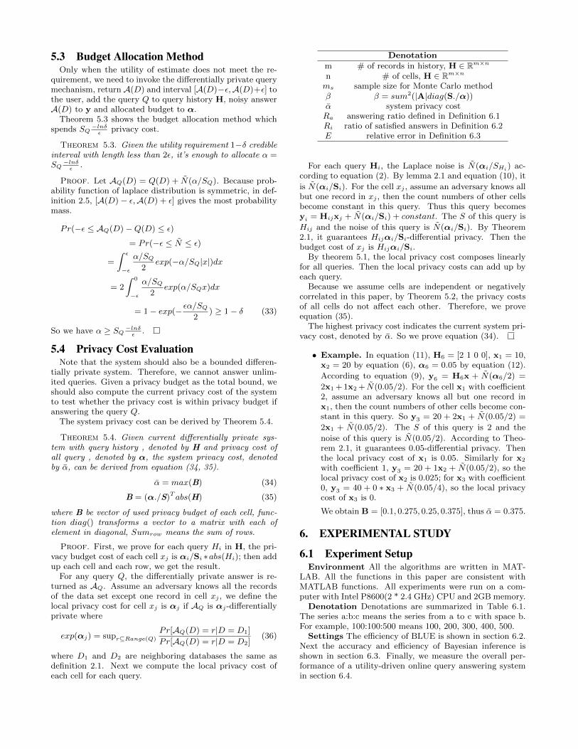
5.3 Budget Allocation MethodOnly when the utility of estimate does not meet the re-

quirement, we need to invoke the differentially private querymechanism, return A(D) and interval [A(D)−ε,A(D)+ε] tothe user, add the query Q to query history H, noisy answerA(D) to y and allocated budget to α.

Theorem 5.3 shows the budget allocation method whichspends SQ

−lnδε

privacy cost.

Theorem 5.3. Given the utility requirement 1−δ credibleinterval with length less than 2ε, it’s enough to allocate α =SQ−lnδε

.

Proof. Let AQ(D) = Q(D) + N(α/SQ). Because prob-ability function of laplace distribution is symmetric, in def-inition 2.5, [A(D)− ε,A(D) + ε] gives the most probabilitymass.

Pr(−ε ≤ AQ(D)−Q(D) ≤ ε)

= Pr(−ε ≤ N ≤ ε)

=

∫ ε

−ε

α/SQ2

exp(−α/SQ|x|)dx

= 2

∫ 0

−ε

α/SQ2

exp(α/SQx)dx

= 1− exp(− εα/SQ2

) ≥ 1− δ (33)

So we have α ≥ SQ−lnδε .

5.4 Privacy Cost EvaluationNote that the system should also be a bounded differen-

tially private system. Therefore, we cannot answer unlim-ited queries. Given a privacy budget as the total bound, weshould also compute the current privacy cost of the systemto test whether the privacy cost is within privacy budget ifanswering the query Q.

The system privacy cost can be derived by Theorem 5.4.

Theorem 5.4. Given current differentially private sys-tem with query history , denoted by H and privacy cost ofall query , denoted by α, the system privacy cost, denotedby α, can be derived from equation (34, 35).

α = max(B) (34)

B = (α./S)T abs(H) (35)

where B be vector of used privacy budget of each cell, func-tion diag() transforms a vector to a matrix with each ofelement in diagonal, Sumrow means the sum of rows.

Proof. First, we prove for each query Hi in H, the pri-vacy budget cost of each cell xj is αi/Si ∗abs(Hi); then addup each cell and each row, we get the result.

For any query Q, the differentially private answer is re-turned as AQ. Assume an adversary knows all the recordsof the data set except one record in cell xj , we define thelocal privacy cost for cell xj is αj if AQ is αj-differentiallyprivate where

exp(αj) = supr⊆Range(Q)

Pr[AQ(D) = r|D = D1]

Pr[AQ(D) = r|D = D2](36)

where D1 and D2 are neighboring databases the same asdefinition 2.1. Next we compute the local privacy cost ofeach cell for each query.

Denotationm # of records in history, H ∈ Rm×nn # of cells, H ∈ Rm×nms sample size for Monte Carlo methodβ β = sum2(|A|diag(S./α))α system privacy costRa answering ratio defined in Definition 6.1Ri ratio of satisfied answers in Definition 6.2E relative error in Definition 6.3

For each query Hi, the Laplace noise is N(αi/SHi) ac-cording to equation (2). By lemma 2.1 and equation (10), it

is N(αi/Si). For the cell xj , assume an adversary knows allbut one record in xj , then the count numbers of other cellsbecome constant in this query. Thus this query becomesyi = Hijxj + N(αi/Si) + constant. The S of this query is

Hij and the noise of this query is N(αi/Si). By Theorem2.1, it guarantees Hijαi/Si-differential privacy. Then thebudget cost of xj is Hijαi/Si.

By theorem 5.1, the local privacy cost composes linearlyfor all queries. Then the local privacy costs can add up byeach query.

Because we assume cells are independent or negativelycorrelated in this paper, by Theorem 5.2, the privacy costsof all cells do not affect each other. Therefore, we proveequation (35).

The highest privacy cost indicates the current system pri-vacy cost, denoted by α. So we prove equation (34).

• Example. In equation (11), H6 = [2 1 0 0], x1 = 10,x2 = 20 by equation (6), α6 = 0.05 by equation (12).

According to equation (9), y6 = H6x + N(α6/2) =

2x1 + 1x2 + N(0.05/2). For the cell x1 with coefficient2, assume an adversary knows all but one record inx1, then the count numbers of other cells become con-stant in this query. So y3 = 20 + 2x1 + N(0.05/2) =

2x1 + N(0.05/2). The S of this query is 2 and the

noise of this query is N(0.05/2). According to Theo-rem 2.1, it guarantees 0.05-differential privacy. Thenthe local privacy cost of x1 is 0.05. Similarly for x2

with coefficient 1, y3 = 20 + 1x2 + N(0.05/2), so thelocal privacy cost of x2 is 0.025; for x3 with coefficient0, y3 = 40 + 0 ∗ x3 + N(0.05/4), so the local privacycost of x3 is 0.

We obtain B = [0.1, 0.275, 0.25, 0.375], thus α = 0.375.

6. EXPERIMENTAL STUDY

6.1 Experiment SetupEnvironment All the algorithms are written in MAT-

LAB. All the functions in this paper are consistent withMATLAB functions. All experiments were run on a com-puter with Intel P8600(2 * 2.4 GHz) CPU and 2GB memory.

Denotation Denotations are summarized in Table 6.1.The series a:b:c means the series from a to c with space b.For example, 100:100:500 means 100, 200, 300, 400, 500.

Settings The efficiency of BLUE is shown in section 6.2.Next the accuracy and efficiency of Bayesian inference isshown in section 6.3. Finally, we measure the overall per-formance of a utility-driven online query answering systemin section 6.4.

6.2 BLUEBecause the linear solution θ = Ay is used in following

steps, running time of BLUE is measured.

6.2.1 Running Time vs. mLet m = 100 : 100 : 2000, n = 100, α be a vector of

random variables uniformly distributed in [0, 1], max(S) =10. The impact of m on the running time is shown in Figure5(left). Running time increases slowly with m.

0 500 1000 1500 20000

0.05

0.1

0.15

0.2

0.25

m

Tim

e

0 500 1000 1500 20000

5

10

15

20

25

n

Tim

e

Figure 5: Running time vs. m(left) and n(right)

6.2.2 Running Time vs. nLet n = 100 : 100 : 2000, α be a vector of random vari-

ables uniformly distributed in [0, 1], max(S) = 10. Be-cause the linear system should be overdetermined, whichmeans m > n, we set m = 2n. From Figure 5(right) weknow that running time rise significantly with n, which ac-tually has verified the motivation of [5] that proposed thePCA(Principle Component Analysis) and maximum entropymethods to boost the speed of this step.

6.3 Bayesian InferenceBy Corollary 4.1, we can derive a bound for ms, ms >

|u|γ2max(u)(1−max(u))+1. However, this is not a sufficient

bound because to implement Monte Carlo method a largenumber of sample size is needed in the first place. Therefore,we set the minimal sample size to be 104. When the derivedbound is larger than 104, let ms be it. So ms = 104 <

( |u|γ2max(u)(1−max(u))+1)?( |u|

γ2max(u)(1−max(u))+1) :

104.

6.3.1 Running Time vs. mLet γ = 0.01, max(S) = 5, n = 100, m = 200 : 100 : 1000.

Figure 6(left) shows that running time of MC rises with m,which complies with Theorem 4.4. But m does not impactthe running time of PC significantly.

200 400 600 800 1000

100

m

Tim

e

MCPC

0 200 400 60010

−2

100

102

104

n

Tim

e

MCPC

Figure 6: Running time vs. m(left) and n(right)

6.3.2 Running Time vs. nLet γ = 0.01, max(S) = 5, m = 500, n = 50 : 50 : 100.

Impact of n is shown in Figure 6(right). Running time PC

increases fast with n. In contrast, parameter n does notaffect running time of MC.

6.3.3 Time and Error of Method PCLet γ = 0.01, max(S) = 5, m = 1000, n = 100, β =

sum2(|Ai|diag(S./α)). Theorem 4.6 implies that runningtime of PC is affected by β. Experimental evaluation inFigure 7(left) confirms the result. The error defined in Def-inition 4.2 is also measured in Figure 7(right). Because wecan set γ in the first place, the error of PC does not increasewith β and any other parameters.

0 2 4 6

x 1011

0

1

2

3

4

5

Tim

e

β

PC

0 2 4 6

x 1011

−1

−0.5

0

0.5

1

1.5

Err

or

β

PC

Figure 7: Time(left) and Error(right) of PC vs. β

6.3.4 Time and Error of Method MCLet n = 100. The sample size ms impacts both time

and error of MC method. Let ms = 105 : 105 : 106. Thetime and error is evaluated in Figure 8 on left and rightrespectively. When ms increases, the running time risesand the error declines, which complies with Theorem 4.4and Corollary4.1.

0 5 10

x 105

0

5

10

15

Tim

e

Sample Size

MC

0 5 10

x 105

0

1

2

3

4

5x 10

−5

Err

or

Sample Size

MC

Figure 8: Time(left) and Error(right) of MC vs.sample Size

6.4 Utility-driven Query Answering SystemData. We use the three data sets: net-trace, social net-

work and search logs, which are the same data sets with [13].Net-trace is an IP-level network trace collected at a majoruniversity; Social network is a graph of friendship relationsin an online social network site; Search logs is a set of searchquery logs over time from Jan.1, 2004 to 2011. The resultsof different data are similar, so we only show net-trace andsearch logs results for lack of space.

Query. User queries may not necessarily obey a certaindistribution. So the question arises how to generate thetesting queries. In our setting, queries are assumed to bemultinomial distributed, which means the probability for thequery to involve cell xj is Pj , where

∑nj=1 Pj = 1. As shown

in Figure 5(right), the running time rises dramatically withn. For efficiency and practicality, we reduce the dimension-ality by assuming some regions of interest, where the cellsare asked more frequently than others. Sparse distributed

queries can also be estimated with the linear solution in [5].Equation (37) shows the probability of each cell.

Pj = 0.9 ∗ 10−floor(j−110

) (37)

where the function floor() rounds the input to the nearestintegers less than it.

To generate a query, we first generate a random numbernt in 1 ∼ 10, which is the # of independent trails of multi-nomial distribution. Then we generate the query from themultinomial distribution, equation (38) shows the probabil-ity of Q.

Pr(Q1 = q1, Q2 = q2, · · · , Qn = qn) =

nt!

q1!q2! · · · qn!P q11 P q22 · · ·P

qnn (38)

where∑j qj = nt.

Finally, we generate 1000 queries for each setting.Utility Requirement We assume each query has differ-

ent utility requirement (ε,δ). Note that ε and δ determinesα and α determines β. Therefore the running time of PCmethod is related to ε and δ. Thus we assume ε has a upperbound 103 and is uniformly distributed.

Metrics Besides system privacy cost α in theorem 5.4,following metrics are used.

For a bounded system, Once the system privacy cost αreaches the overall privacy budget, then the system cannotanswer further queries. To measure this, we define the ratioof answered queries as below. In another word, it indicatesthe capacity(or life span) of a system.

Definition 6.1. Under the bound of overall privacy bud-get, given a set of queries Q with utility requirements, theanswering ratio Ra is

Ra =(# of answers : Pr(L ≤ θ ≤ U) ≥ 1− δ)

(# of all queries)(39)

Among all the answered queries, we want to know theaccuracy of the returned answer. We use following two met-rics. 1. Ri is defined to show whether the returned intervalreally contain the original answer; 2. E is the distance be-tween returned answer and true answer. It is easy to provethat if # of answered queries approaches to infinity, Ri con-verges to confidence level.

Definition 6.2. For a set of queries with utility require-ments, the credible intervals [L,U ] are returned. Ratio ofreliability Ri is defined as follows:

Ri =

∑i∈answered queries(# of answers : L ≤ θ ≤ L+ 2εi)

# of all answered queries(40)

Note that in the experiment we know the true value of θ.Therefore, Ri can be derived.

Definition 6.3. For each query with (ε, δ) requirement,

a returned answer θ is provided by the query answering sys-tem. If the original answer is θ, the relative error is definedto reflect the accuracy of θ:

E =

∑i∈answered queries(|θi − θi|/(2εi))# of all answered queries

(41)

α

200 400 600 800 10000

1

2

3

4

5

improved baselineinference

200 400 600 800 10000

1

2

3

4

5


E

200 400 600 800 10000

0.1

0.2

0.3

0.4

0.5

0.6


200 400 600 800 10000

0.1

0.2

0.3

0.4

0.5

0.6


Ri

200 400 600 800 10000.6

0.7

0.8

0.9

1

1.1


200 400 600 800 10000.6

0.7

0.8

0.9

1

1.1


Figure 9: Evaluation of unbounded setting for net-trace(left) and search logs(right). All x-axes repre-sent # of queries. First row shows α; second rowshows E; third row shows Ri. Improved baselinemeans baseline system with dynamic budget alloca-tion.

In summary, α indicates the system privacy cost; Ra in-dicates the capacity(or life span) of a system; Ri indicatesthe confidence level of returned credible interval [L,U ]; E

indicates the accuracy of the point estimation θ.Settings We use PC inference method for efficiency. The

above four metrics are evaluated in two settings. In thefirst setting, the overall privacy budget is unbounded. ThusRa = 1 because all queries can be answered. Also a setof history queries, known as H, is also given in advance.Although it is not a realistic setting, we can measure howthe system can save privacy budget by our method. In thesecond setting, the privacy budget is bounded. ThusRa ≤ 1.

6.4.1 Unbounded SettingA hierarchical partitioning tree[13] is given using 0.3-differential

privacy as query history to help infer queries. Let 2ε be uni-formly distributed in [50, 103], δ = 0.2.

We improve the baseline interactive query-answering sys-tem with our budget allocation method(Theorem 5.3), thenit can save privacy budget and achieve better utility. Theimproved baseline systems are compared with or without theBayesian inference technique. Because we don’t allocate pri-vacy budget if the estimate can satisfy utility requirement,privacy budget can be saved furthermore. In Figure 9, Riand E also become better using inference technique.6.4.2 Bounded Setting

For a bounded system, we use both budget allocation andBayesian inference to improve the performance. Let theoverall privacy budget be 1; let 2ε be uniformly distributedin [1, 103], δ = 0.2. Figure 10 shows the performance.

Ra

200 400 600 800 10000

0.2

0.4

0.6

0.8

1


200 400 600 800 10000

0.2

0.4

0.6

0.8

1


E

200 400 600 800 10000

0.5

1

1.5

improved baselineinferenceOLS solution

200 400 600 800 10000

0.5

1

1.5

improved baselineinferenceOLS solution

Ri

200 400 600 800 10000.6

0.7

0.8

0.9

1

1.1


200 400 600 800 10000.6

0.7

0.8

0.9

1

1.1


Figure 10: Evaluation of bounded setting for net-trace(left) and search logs(right). All x-axes repre-sent # of queries. First row shows Ra; second rowshows E; third row shows Ri. Improved baselineand OLS solution are improved by our method ofdynamic budget allocation.

Because α reaches the overall privacy budget for about100 queries, further queries cannot be answered by improvedbaseline system. But for our inference system, they may alsobe answered by making inference of history queries. Thiscan increase Ra. Also E and Ri is better than improvedbaseline system. We also compared E of OLS solution[18]with budget allocation method. In our setting, the resultis better than OLS solution because OLS is not sensitive toutility requirement and privacy cost α. For example, if aquery requires high utility, say 2ε = 5, then a big α is allo-cated and a small noise is added to the answer. But OLSsolution treats all noisy answers as points without any prob-ability properties. Therefore, this answer with small noisecontributes not so much to the OLS estimate. Then accord-ing to Equation (41), E becomes lager than the inferenceresult.

Note that E and Ri is not as good as Figure 9. Thereare two reasons. First, we don’t have any query historyat the beginning. So the system must build a query his-tory to make inference for new queries. Second, when αreaches the overall privacy budget, the query history we haveis actually the previous answered queries, which are gener-ated randomly. Compared with the hierarchical partitioningtree[13], it may not work so well. We believe delicately de-signed query history[27, 18, 13] or auxiliary queries[25] canimprove our system even better, which can be investigatedin further works.

7. REFERENCES[1] H. Anton and C. Rorres. Introduction to Probability

Models, Tenth Edition. John Wiley and Sons, Inc, 2005.

[2] A. Blum, C. Dwork, F. McSherry, and K. Nissim. Practicalprivacy: the sulq framework. pages 128–138. PODS, 2005.

[3] A. Blum, K. Ligett, and A. Roth. A learning theoryapproach to non-interactive database privacy. Stoc’08:Proceedings of the 2008 Acm International Symposium onTheory of Computing, pages 609–617, 2008. 14th AnnualACM International Symposium on Theory of ComputingMAY 17-20, 2008 Victoria, CANADA.

[4] L. Chao and M. Gerome. An adaptive mechanism foraccurate query answering under differential privacy. InProceedings of the 2012 VLDB, VLDB ’12, 2012.

[5] S. Chen, Z. Shuigeng, and S. S. Bhowmick. Integratinghistorical noisy answers for improving data utility underdifferential privacy. In Proceedings of the 2011 EDBT,EDBT ’12, 2012.

[6] B. Ding, M. Winslett, J. Han, and Z. Li. Differentiallyprivate data cubes: optimizing noise sources andconsistency. In SIGMOD, 2011.

[7] C. Dwork. Differential privacy. Automata, Languages andProgramming, Pt 2, 4052:1–12, 2006. Bugliesi, M Prennel,B Sassone, V Wegener, I 33rd International Colloquium onAutomata, Languages and Programming JUL 10-14, 2006Venice, ITALY.

[8] C. Dwork. Differential privacy: a survey of results. InProceedings of the 5th international conference on Theoryand applications of models of computation, TAMC, 2008.

[9] C. Dwork. A firm foundation for private data analysis.Commun. ACM., 2010.

[10] C. Dwork, F. McSherry, K. Nissim, and A. Smith.Calibrating noise to sensitivity in private data analysis.pages 265–284. Proceedings of the 3rd Theory ofCryptography Conference, 2006.

[11] T. Eltoft, T. Kim, and T.-W. Lee. On the multivariatelaplace distribution. In IEEE Signal Processing Letters,pages 300–303, 2006.

[12] C. George and R. L.Berger. Statistical Inference 002edition . Duxbury Press, 2001.

[13] M. Hay, V. Rastogiz, G. Miklauy, and D. Suciu. Boostingthe accuracy of differentially-private histograms throughconsistency. VLDB, 2010.

[14] U. Kchler and S. Tappe. On the shapes of bilateral gammadensities. Statistics & Probability Letters,78(15):2478–2484, October 2008.

[15] D. Kifer and A. Machanavajjhala. No free lunch in dataprivacy. In Proceedings of the 2011 international conferenceon Management of data, SIGMOD ’11, pages 193–204, NewYork, NY, USA, 2011. ACM.

[16] S. Kotz, T. J. Kozubowski, and K. Podgorski. The Laplacedistribution and generalizations. Birkhauser, 2001.

[17] J. Lee and C. Clifton. How much is enough? choosing fordifferential privacy. In ISC, pages 325–340, 2011.

[18] C. Li, M. Hay, V. Rastogi, G. Miklau, and A. McGregor.Optimizing linear counting queries under differentialprivacy. In PODS ’10: Proceedings of the twenty-ninthACM SIGMOD-SIGACT-SIGART symposium onPrinciples of database systems of data, pages 123–134, NewYork, NY, USA, 2010. ACM.

[19] K. M and H. J, W. Data mining: concepts and techniques,Second Edition. MorganKaufman, 2006.

[20] McSherry. Privacy integrated queries: an extensibleplatform for privacy-preserving data analysis. In SIGMOD’09: Proceedings of the 35th SIGMOD internationalconference on Management of data, pages 19–30, NewYork, NY, USA, 2009. ACM.

[21] F. McSherry and K. Talwar. Mechanism design viadifferential privacy. 48th Annual Ieee Symposium onFoundations of Computer Science, Proceedings, pages94–103, 2007. 48th Annual IEEE Symposium onFoundations of Computer Science OCT 20-23, 2007Providence, RI.

[22] V. Rastogi, M. Hay, G. Miklau, and D. Suciu. Relationship

privacy: output perturbation for queries with joins. InProceedings of the twenty-eighth ACMSIGMOD-SIGACT-SIGART symposium on Principles ofdatabase systems, PODS ’09, pages 107–116, New York,NY, USA, 2009. ACM.

[23] A. Smith. Efficient, differentially private point estimators.CoRR, abs/0809.4794, 2008.

[24] O. Williams and F. McSherry. Probabilistic inference anddifferential privacy. In J. Lafferty, C. K. I. Williams,J. Shawe-Taylor, R. Zemel, and A. Culotta, editors,Advances in Neural Information Processing Systems 23,pages 2451–2459. 2010.

[25] X. Xiao, G. Bender, M. Hay, and J. Gehrke. ireduct:differential privacy with reduced relative errors. InProceedings of the 2011 international conference onManagement of data, SIGMOD ’11, pages 229–240, NewYork, NY, USA, 2011. ACM.

[26] X. Xiao, G. Wang, and J. Gehrke. Differential privacy viawavelet transforms. In ICDE, pages 225–236, 2010.

[27] Y. Xiao, L. Xiong, and C. Yuan. Differentially Private DataRelease through Multidimensional Partitioning. volume6358, pages 150–168, 2010. 7th VLDB Workshop on SecureDate Management, Singapore, SINGAPORE, SEP 17,2010.

8. APPENDIX

H matrix of query history;x original count of each cell;

y noisy answer of H, y = Hx + N;α privacy budget for one query;α privacy cost for the whole system;L and U upper and lower bound of credible interval;ε ε = (U − L)/2;δ 1− δ is the confidence level;α privacy cost of each row in H;S the sensitivity of each row in H;θ or Q(D) original answer of query Q;

N(α) Laplace noise with parameter α;AQ(D) returned answer of Laplace mechanism:

θ = θ + N(α/S);

θ observation of a query: θ = θ +N ;

θ estimated answer of Q(D);

N noise vector of y;

Bayesian Inference under Differential Privacy

Documents

Transcript of Bayesian Inference under Differential Privacy