Bayesian Inference in the Modern Design of Experiments · American Institute of Aeronautics and...

American Institute of Aeronautics and Astronautics

1

Bayesian Inference in the Modern Design of Experiments

Richard DeLoach*

NASA Langley Research Center, Hampton, VA, 23681

This paper provides an elementary tutorial overview of Bayesian inference and its

potential for application in aerospace experimentation in general and wind tunnel testing in

particular. Bayes’ Theorem is reviewed and examples are provided to illustrate how it can

be applied to objectively revise prior knowledge by incorporating insights subsequently

obtained from additional observations, resulting in new (posterior) knowledge that combines

information from both sources. A logical merger of Bayesian methods and certain aspects of

Response Surface Modeling is explored. Specific applications to wind tunnel testing,

computational code validation, and instrumentation calibration are discussed.

Nomenclature

= angle of attack, Type I inference error probability

= angle of sideslip, Type II inference error probability

d = order of polynomial

F = generic response symbol

i, j = index variables

k = number of independent variables

K = number of regressors in a polynomial model

p = number of parameters in a polynomial model, including intercept

p′ = maximum acceptable inference error probability

p00 = probability that if a candidate model term was rejected in the last experiment, it will be rejected in the

next replicate of that experiment

p01 = probability that if a candidate model term was rejected in the last experiment, it will be retained in the


p10 = probability that if a candidate model term was retained in the last experiment, it will be rejected in the


p11 = probability that if a candidate model term was retained in the last experiment, it will be retained in the


0 = proportion of times that a candidate model term is rejected in a series of replicated experiments

1 = proportion of times that a candidate model term is retained in a series of replicated experiments

RSM = Response Surface Methods/Models/Modeling

X = design matrix

alternative hypothesis = assertion that a significant difference exists between an estimated response and

a given reference

coding = linear transformation of variables into a range convenient for processing

conditional probability = probability that one event will occur, given the occurrence of another event

confidence interval = precision interval when n = infinity

explained SS = sum of squares attributable to known causes

F-Value = ratio of mean square for an effect to residual mean square

factor = an independent variable; e.g. angle of attack

factor level = a specific value for an independent variable; e.g., angle of attack = 2°

graduating function = low-order approximation to true but unknown response function

hierarchy = condition in which higher order terms are accompanied by component lower-order term

inference = decision to reject either a null hypothesis or its corresponding alternative

inference space = a coordinate system in which one axis is assigned to each independent variable

*Senior Research Scientist, NASA Langley Research Center, Hampton, VA. AIAA Senior Member.

https://ntrs.nasa.gov/search.jsp?R=20080008574 2018-06-13T02:04:00+00:00Z


2

interaction effect = change in effect due to change in factor level from low to high

joint probability = probability of two events both occurring

LOF = lack of fit

main effect = change in response due to change in factor level from low to high

marginal probability = probability that an event will occur, independent of whether another event occurs

MDOE = Modern Design of Experiments

mean square = ratio of sum of squares to degrees of freedom; variance

null hypothesis = assertion than no difference exists between an estimated response and a

given reference

OFAT = One Factor At a Time

orthogonal = state in which regressors are all mutually independent

regressor = term in a regression model

residual = difference between measurement and some reference

residual mean square = residual sum of squares divided by residual degrees of freedom

residual SS = difference between total sum of squares and explained sum of squares

response surface model = mathematical relationship between a response variable and multiple

independent variables

significance = risk of erroneously rejecting a null hypothesis

site = a point within an inference space representing some unique combination of

factor levels

t-limit = minimum acceptable signal-to-noise ratio

t-value = measured quantity expressed as multiple of standard error in measurement

Type-I inference error = erroneous rejection of a null hypothesis

Type-II inference error = erroneous rejection of an alternative hypothesis

I. Introduction

t is common to approach the analysis of information obtained in a response surface modeling experiment such as a

wind tunnel test or a force balance calibration as if it stands alone, notwithstanding the fact that considerable prior

information may exist on the subject under study in the experiment. A wind tunnel test may feature the replication of

measurements acquired earlier on the same model, either in that facility or in another wind tunnel. An instrument

undergoing a calibration may have been calibrated numerous times before. While it is not uncommon to compare

current and prior results in such circumstances, such a comparison seldom extends beyond a subjective assessment

that the agreement is generally satisfactory, or that it is sufficiently poor to be of concern. We do not usually exploit

the fact that earlier experiments have yielded results that might be combined with our most recent findings to

produce a composite outcome that reflects both the current and prior work.

There are several reasons to recommend such an integration of prior and current results when the opportunity

presents itself to do so. By including prior data in the current analysis, the researcher avails himself of additional

degrees of freedom that can reduce inference error risk in the current experiment and increase the precision with

which results can be reported. That is to say, such a strategy has the potential to significantly reduce uncertainty,

thereby improving the quality of the final result. Furthermore, these benefits can be obtained ―for free,‖ in that the

expense of obtaining them has already been incurred, either by the researcher himself in a prior experiment or by

some other research program entirely. In the former case, the merging of prior and current experimental findings

results in an averaging down of the researcher’s per-test costs. In the latter case, it results in a cost-effective

leveraging of findings published in the literature or shared directly by colleagues who are able to do so.

An objective, systematic mechanism for merging current and prior experimental results is necessary to take

advantage of this potential opportunity for quality improvement and average cost reduction. Fortunately, this

mechanism is available in the form of Bayesian revision in statistical analysis. Bayesian revision can be applied to a

statistical representation of the random variables comprising any experimental data sample to generate revised

estimates for the location and dispersion metrics that characterize the probability distributions of such data, which

reflect both prior and current information. This paper proposes the merger of such Bayesian methods with the

response surface methods that are a key element of an integrated experiment design, execution, and analysis process

known at NASA Langley Research Center as the Modern Design of Experiments.

The remainder of this paper is organized into five sections. Section II discusses the role of formal inference in

the Modern Design of Experiments. Section III reviews Bayes’ Theorem and gives examples of Bayesian inference.

Section IV describes potential applications of Bayesian inference to response surface modeling experiments. Section

I


3

V discusses certain aspects of Bayesian inference that distinguish it from conventional inference methods. Section

VI provides some concluding remarks.

II. The Role of Formal Inference in the Modern Design of Experiments

The Modern Design of Experiments (MDOE) is an adaptation of industrial designed experiments that focuses on

the special requirements of empirical aerospace research, including wind tunnel testing.1 It was first applied to wind

tunnel testing at NASA Langley Research Center in 1997 and has since been used in over 100 major experiments as

a means of delivering higher quality and greater productivity than conventional one factor at a time (OFAT) testing

methods used traditionally in experimental aeronautics. Differences between MDOE and OFAT methods for wind

tunnel testing stem primarily from contrasting views of the objective of this activity. Colloquially stated,

conventional OFAT practitioners conduct wind tunnel tests to acquire data, while MDOE practitioners conduct wind

tunnel tests to acquire knowledge. That is, the OFAT practitioner’s typical test strategy is to directly measure system

responses such as forces and moments for as many independent variable (factor) combinations of interest as

resource constraints will allow, while the MDOE practitioner’s typical strategy is to make some relatively small

number of measurements that is nonetheless ample to develop a mathematical model that can adequately predict

responses for all factor combinations of interest, and to make no more measurements than that.

MDOE predictions are based on response surface models fitted by regression or other means from a sample of

experimental data. The size of this sample is minimized to reduce direct operating cost and cycle time as noted, and

the selection and acquisition order of the individual data points are optimized to reduce uncertainty in predictions

made from models that are fitted from the data.2,3

Fitting a regression model to a relatively small data sample offers certain advantages over the traditional OFAT

exhaustive enumeration strategy that requires every interesting combination of independent variable levels to be

physically set. Besides the obvious cost and cycle-time reductions achievable by minimizing data volume, the

modeling approach enables interpolation, so that response estimates can be made for many other factor

combinations than those physically set in the test.

Low-order polynomials are a convenient and common form of response model fitted from experimental data.

Such a model can be regarded as a truncated Taylor series representation of the true but unknown functional

relationship between some response of interest (a force or moment, say), and the independent variables that

influence that response (angle of attack, Mach number, control surface deflections, etc). Often such models are fitted

over a limited range of the independent variables so that the resulting model—called a graduating function—can be

regarded as a mathematical ―French curve‖ that fits the data adequately in this range. Other models are then

developed for other ranges of the variables. By restricting the range of the independent variables sufficiently, an

adequate fit to the data can be secured for arbitrarily low-order graduating functions. Typically we seek a reasonable

compromise between the order of the fitting model and the range of independent variables to be fitted.

Progress is made in an MDOE experiment through an iterative process in which a proposed model is subjected to

criticism intended to test certain assumptions upon which the validity of the model rests. Typically this criticism

takes the form of various tests applied to model residuals, which can be expected to contain no information for a

well-fitted model, and which reveal trends and other information when the model is an inadequate representation of

the underlying data. Likewise, certain distributional assumptions of the residuals are commonly tested.

Information revealed in an analysis of the residuals may suggest improvements to the model, or the need to

acquire additional data to fit a more complex function of the independent variables. A revised model is then

produced, which is again subjected to criticism. This process continues until the researcher is satisfied that the model

is adequate for a particular purpose defined during the design of the experiment. In a wind tunnel test, that purpose

typically is to predict measured responses within a specified tolerance and with an acceptable level of confidence.

The tolerances and confidence levels are documented as part of the MDOE experiment design process.

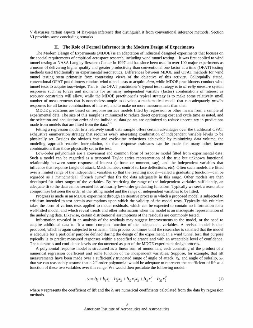
A polynomial response model is structured as a linear sum of monomials, each consisting of the product of a

numerical regression coefficient and some function of the independent variables. Suppose, for example, that lift

measurements have been made over a sufficiently truncated range of angle of attack, x1, and angle of sideslip, x2,

that we can reasonably assume that a 2nd

-order polynomial would be adequate to represent the coefficient of lift as a

function of these two variables over this range. We would then postulate the following model:

2 2

0 1 1 2 2 12 1 2 11 1 22 2y b b x b x b x x b x b x (1)

where y represents the coefficient of lift and the bi are numerical coefficients calculated from the data by regression

methods.


4

Regression is simply a defined computational process that will generate a set numerical regression coefficients

for this model without regard for physical reality. For example, if there is no interaction between x1 and x2 (that is, if

the effect on y of a given change in x1 is the same no matter the value of x2), then the x1x2 cross term would be

superfluous and the true value of the b12 coefficient in this model would be zero. Unfortunately, unexplained

variance present in every experimental data sample results in uncertainty in the estimates of regression coefficients.

The result is that, except for sheer coincidence, the fitted coefficients of each of the six terms in a second-order

polynomial function of two independent variables will be non-zero, even if the physical phenomenon represented by

a given term does not occur in nature.

The researcher is motivated to minimize the number of terms in a response surface model by dropping all terms

for which the true value of the regression coefficient is zero. This is so for a number of reasons. One is that since

each term in the model carries some uncertainty due to the experimental error in its regression coefficient, the

smaller the number of such imperfect terms that are summed to form a response estimate, the smaller the uncertainty

will be in that estimate. Indeed, it can be shown4 that the prediction variance averaged across all points used to

generate a well-fitted regression model is simply

2p

Var yn

(2)

where p is the number of terms in the model including the intercept (so six for the present model) and n is the

number of points in the data sample used to generate the model. We note in passing that n ≥ p is a condition for

fitting a model so that in the limiting case for which n = p and there are just enough points to fit the model, the

average model prediction variance is just 2, the intrinsic variance in the data. However, in the more general case in

which n > p so that there are residual degrees of freedom available, the average prediction variance is less than the

intrinsic variance of the data. This is an additional argument in favor of response surface methods for estimating

system responses, rather than the individual measurements that characterize OFAT testing.

Beyond reducing model prediction variance, the researcher is motivated to develop compact response models in

order to clarify the underlying physics. In the example already cited, if there is no physical interaction between the

two independent variables in Eq. (1), then retaining such an interaction term in the model simply adds unnecessary

clutter.

The process of response surface model building reduces to a series of decisions, or inferences, with respect to

whether the regression coefficient of a given candidate term in a proposed model conveys information about the true

system response, or whether it is due to nothing more than experimental error. Formally, we establish a null

hypothesis for each model term except the intercept, declaring it to be superfluous. We only reject this null

hypothesis (and therefore retain the candidate term in the model) if there is compelling objective evidence to do so.

The decision of whether or not to reject the null hypothesis for a given term in a proposed model is made with

the aid of a reference probability distribution. This distribution reflects the dispersion in experimental estimates of

the regression coefficient, and is therefore related to the ―noise‖ in an experimental result. We reject the null

hypothesis only when the magnitude of the estimated regression coefficient is sufficiently different from zero that

we can infer that it is not zero with an acceptably low probability of an inference error. Stated another way, we

demand a certain minimum signal-to-noise ratio as a condition for rejecting the null hypothesis.

Reference distributions are illustrated in Fig. 1 for two regression coefficients. We generally appeal to the

Central Limit Theorem to support an assumption that these distributions are Gaussian. If we infer that the true value

of the ith

regression coefficient is indeed greater than zero, then the probability of an error in this inference, pi, is

20

2

1exp

22

i

i

ii

x bp dx

(3)

which is simply the area under the probability density function to the left of zero, where i is the standard deviation

of this distribution. Obviously, the further from zero that bi is, the smaller is the probability, pi, of making an

inference error by rejecting the null hypothesis. Such an error would result in retaining a non-existent term in the

response model, and is known as a Type I inference error. For example, if in Eq. (1) we were to retain the b12x1x2

term when there was in fact no physical interaction between x1 and x2, then we would have made this type of

inference error.


5

To make an inference for the regression

coefficient of the ith

candidate model term, we

simply need an estimate of the coefficient, bi,

and the standard error in estimating it, i, as

well as some criterion for an acceptable

inference error probability. From the first two

quantities we compute the inference error

probability using Eq. (3), and then compare this

to the criterion, which can be arbitrarily small

but not zero.

The regression coefficients and their

standard errors are a function of the design

matrix, which represents a straightforward

extension of the familiar test matrix that lists

independent variable levels to be set for each

data point to be acquired in an experiment. Just

as in the case of the standard test matrix, there

is one row in the design matrix for each data

point. Each column corresponds to a different

term in the regression model to be fitted. The

elements of the design matrix in the columns

corresponding to first order terms in the model

are the same as in the conventional test matrix.

Higher-order columns are generated from the first order columns via term-by-term manipulations of the lower-order

terms. For example, the elements of the x1x2 column are generated by simply multiplying the x1 and x2 levels for

each data point. Likewise, columns for quadratic terms are generated by squaring the corresponding elements in the

first-order columns, and so on. Before the design matrix is generated the variables are commonly scaled and

centered by a linear transformation that maps them into a range from -1 to +1, with ―0‖ corresponding to the center

of the range. This minimizes certain round-off errors that can occur when the numerical magnitudes of different

variables in physical units are considerably different (angle of attack on the order of ones to tens and Reynolds

numbers in the range of millions, for example).

The reader is referred to standard texts on regression analysis and response surface modeling4–7

for additional

details on the construction of the design matrix, X. Suffice it to say that two points are key with respect to the design

matrix: 1) for a given measurement environment, the regression coefficients and their standard errors are completely

defined by the design matrix and the resulting vectors of measured responses, which means that inference errors are

directly impacted by the nature of the design matrix, and 2) the structure of the design matrix is defined by the

researcher prior to the test. This is the reason that there is so much potential to influence the quality and productivity

of a wind tunnel test or any other type of experiment by the design of the experiment.

A 1 × p vector of regression coefficients, b, can be computed directly from the p × n design matrix, X, and the

1 × n vector of corresponding response measurements, Y, where p is the number of terms in the fitted model

including the intercept term as before, and n is the number of points used to fit the response model:

-1

b = X X X Y (4)

The standard error for each regression coefficient comes from the covariance matrix, C, computed by inverting

the product of the transpose of the design matrix (X’) and the design matrix, X, then multiplying every term by 2,

the unexplained variance in the response measurements.

1 2

C X X (5)

The covariance matrix is a p × p square matrix. The standard error for the ith

regression coefficient is simply the

square root of the iith

(diagonal) element of this matrix. These represent the standard deviations of the reference

Figure 1. The magnitude of two regression coefficients,

showing dispersion in their experimental estimates

(reference distributions). We reject the null hypothesis for

b2 but not for b

1.


6

distributions used to infer whether or not to reject the null hypothesis that a given candidate term in the model

should be eliminated. See Fig. 1.

This discussion has highlighted the role that probability and statistical inference plays in the response surface

methods used in an MDOE analysis. Inference error probabilities are estimated for each candidate regression

coefficient via Eqs. (3), (4), and (5), and compared with inference error criteria developed in the experiment design

phase. By one common convention, the null hypothesis is only rejected if the corresponding probability of an

inference error is no greater than 0.05. By this criterion, we require the estimated regression coefficient’s signal to

noise ratio to be large enough that we can say with 95% confidence that it is not zero, and that the corresponding

term does therefore belong in the regression model. Coefficients with a smaller signal to noise ratio may in fact be

non-zero, but those terms are rejected from the model on the grounds that the coefficients are not large enough for us

to say with confidence that they belong.

Table 1 describes a response surface model generated in a recent wind tunnel test at Langley Research Center.

This model represents lift coefficient as a function of the angles of attack and sideslip over ranges of those variables

that were sufficiently constrained that it was believed a good fit could be achieved with a full second-order response

model in the two independent variables.

Recall that we progress in an MDOE analysis by postulating a candidate model and then subjecting it to

criticism. We conduct a critical examination of the candidate model with the intent of identifying ways to improve

it. In the case of the lift model represented in Table 1, we see that if we reject the null hypothesis for the first-order

angle of attack term, the error probability associated with that inference is negligible (< 0.0001). We conclude that

we would be very unlikely to improve the model (and would therefore be at some risk of degrading it) if we failed to

include the first-order angle of attack term in the model. This is consistent with experience and subject matter

expertise, from which we realize that pre-stall lift is very nearly a linear function of angle of attack. Likewise,

decisions to retain the first- and second-order sideslip angle terms seem to be well justified. However, two of the

five regressors have inference error probabilities that exceed our 0.05 criterion for rejecting the null hypothesis and

retaining the term. These are the pure quadratic angle of attack term with an inference error probability of 0.0842,

and the interaction term with an inference error probability of 0.9363.

We interpret these probabilities as descriptive of the chance that a coefficient of the size estimated from the data

could have been computed strictly as the result of experimental error. This probability is especially high for the

interaction term, reflecting the fact that our estimate of the coefficient for that term is two orders of magnitude

smaller than the smallest coefficient for any other regressor in the model and only represents 0.08 of one standard

deviation, so a very small signal-to-noise ratio. We therefore tentatively drop both of these terms to produce a

reduced model of the following form

2

0 1 1 2 2 22 2y b b x b x b x (6)

By Eq. (2), reducing the parameter count, p, from six to four will have reduced that component of the prediction

variance due to random error by a third. However, if eliminating one or both of these two terms ultimately proves to

Table 1. Initial Regression Model.

Factor Regression Coefficient Std Err of

Coefficient

Inference Error Probability

if Null Hypothesis Rejected

Intercept 0.5389 5.48E-04 --

1x , Angle of Attack 9.099E-02 5.48E-04 <0.0001

2x , Angle of Sideslip 1.967E-03 5.48E-04 0.0050

2

1x -1.051E-03 5.48E-04 0.0842

2

2x 3.188E-03 5.48E-04 0.0002

1 2x x 6.35E-05 7.75E-04 0.9363


7

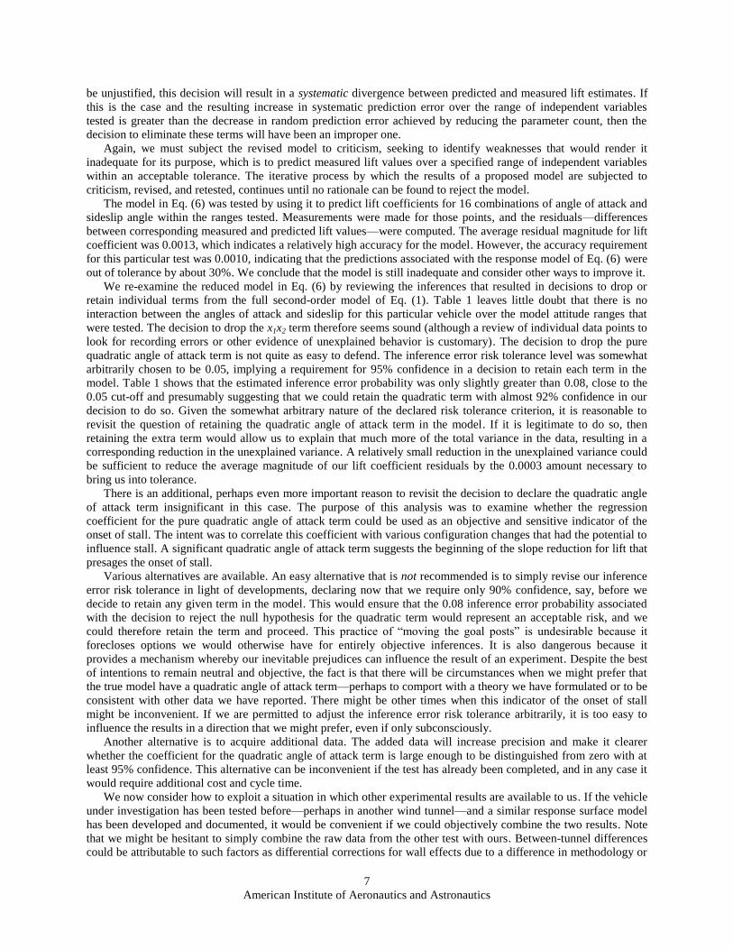
be unjustified, this decision will result in a systematic divergence between predicted and measured lift estimates. If

this is the case and the resulting increase in systematic prediction error over the range of independent variables

tested is greater than the decrease in random prediction error achieved by reducing the parameter count, then the

decision to eliminate these terms will have been an improper one.

Again, we must subject the revised model to criticism, seeking to identify weaknesses that would render it

inadequate for its purpose, which is to predict measured lift values over a specified range of independent variables

within an acceptable tolerance. The iterative process by which the results of a proposed model are subjected to

criticism, revised, and retested, continues until no rationale can be found to reject the model.

The model in Eq. (6) was tested by using it to predict lift coefficients for 16 combinations of angle of attack and

sideslip angle within the ranges tested. Measurements were made for those points, and the residuals—differences

between corresponding measured and predicted lift values—were computed. The average residual magnitude for lift

coefficient was 0.0013, which indicates a relatively high accuracy for the model. However, the accuracy requirement

for this particular test was 0.0010, indicating that the predictions associated with the response model of Eq. (6) were

out of tolerance by about 30%. We conclude that the model is still inadequate and consider other ways to improve it.

We re-examine the reduced model in Eq. (6) by reviewing the inferences that resulted in decisions to drop or

retain individual terms from the full second-order model of Eq. (1). Table 1 leaves little doubt that there is no

interaction between the angles of attack and sideslip for this particular vehicle over the model attitude ranges that

were tested. The decision to drop the x1x2 term therefore seems sound (although a review of individual data points to

look for recording errors or other evidence of unexplained behavior is customary). The decision to drop the pure

quadratic angle of attack term is not quite as easy to defend. The inference error risk tolerance level was somewhat

arbitrarily chosen to be 0.05, implying a requirement for 95% confidence in a decision to retain each term in the

model. Table 1 shows that the estimated inference error probability was only slightly greater than 0.08, close to the

0.05 cut-off and presumably suggesting that we could retain the quadratic term with almost 92% confidence in our

decision to do so. Given the somewhat arbitrary nature of the declared risk tolerance criterion, it is reasonable to

revisit the question of retaining the quadratic angle of attack term in the model. If it is legitimate to do so, then

retaining the extra term would allow us to explain that much more of the total variance in the data, resulting in a

corresponding reduction in the unexplained variance. A relatively small reduction in the unexplained variance could

be sufficient to reduce the average magnitude of our lift coefficient residuals by the 0.0003 amount necessary to

bring us into tolerance.

There is an additional, perhaps even more important reason to revisit the decision to declare the quadratic angle

of attack term insignificant in this case. The purpose of this analysis was to examine whether the regression

coefficient for the pure quadratic angle of attack term could be used as an objective and sensitive indicator of the

onset of stall. The intent was to correlate this coefficient with various configuration changes that had the potential to

influence stall. A significant quadratic angle of attack term suggests the beginning of the slope reduction for lift that

presages the onset of stall.

Various alternatives are available. An easy alternative that is not recommended is to simply revise our inference

error risk tolerance in light of developments, declaring now that we require only 90% confidence, say, before we

decide to retain any given term in the model. This would ensure that the 0.08 inference error probability associated

with the decision to reject the null hypothesis for the quadratic term would represent an acceptable risk, and we

could therefore retain the term and proceed. This practice of ―moving the goal posts‖ is undesirable because it

forecloses options we would otherwise have for entirely objective inferences. It is also dangerous because it

provides a mechanism whereby our inevitable prejudices can influence the result of an experiment. Despite the best

of intentions to remain neutral and objective, the fact is that there will be circumstances when we might prefer that

the true model have a quadratic angle of attack term—perhaps to comport with a theory we have formulated or to be

consistent with other data we have reported. There might be other times when this indicator of the onset of stall

might be inconvenient. If we are permitted to adjust the inference error risk tolerance arbitrarily, it is too easy to

influence the results in a direction that we might prefer, even if only subconsciously.

Another alternative is to acquire additional data. The added data will increase precision and make it clearer

whether the coefficient for the quadratic angle of attack term is large enough to be distinguished from zero with at

least 95% confidence. This alternative can be inconvenient if the test has already been completed, and in any case it

would require additional cost and cycle time.

We now consider how to exploit a situation in which other experimental results are available to us. If the vehicle

under investigation has been tested before—perhaps in another wind tunnel—and a similar response surface model

has been developed and documented, it would be convenient if we could objectively combine the two results. Note

that we might be hesitant to simply combine the raw data from the other test with ours. Between-tunnel differences

could be attributable to such factors as differential corrections for wall effects due to a difference in methodology or


8

a difference in test section geometry, differences in instrumentation, differences in the fidelity of the model, etc.

Such between-tunnel differences have the potential to add enough additional unexplained variance to an analysis of

both sets of data combined, that the subtle effects we seek to illuminate could be lost in the ensuing noise.

As an alternative, consider a case in which the first experiment has been subjected to a response surface analysis,

and inferences have been made about whether to retain or reject terms in the response model for lift coefficient

developed in that model. We describe in the next section how an application of Bayes’ Theorem can objectively

combine the results of two such experiments.

III. Bayes’ Theorem and Bayesian Inference

We adopt a standard notation by using P(A|B) to represent the conditional probability that event ―A‖ will occur,

given that event ―B‖ has occurred. We say that the probability of ―A‖ is conditional on ―B‖ in this case. For

example, event ―A‖ might represent a regression coefficient in a candidate response model being non-zero. Event

―B‖ might be the acquisition of some sample of data. In that case, P(A|B) represents the probability that the

coefficient is significant, given the data sample.

In general, P(A|B) is not the same as P(B|A); however, they are related to each other through a relatively simple

relationship comprising Bayes’ Theorem. Bayes’ Theorem can be exploited to objectively revise early conclusions

in light of new evidence, as will be shown in this section. For example, we originally concluded in the previous

section that the pure quadratic angle of attack term in a candidate model for lift coefficient could be rejected, and we

have now postulated additional evidence in the form of a second wind tunnel test. The question is, does the

additional evidence indicate that we should revise our original belief about the significance (or lack thereof) of the

quadratic angle of attack term for this model? To address this question, we review Bayes’ Theorem and give some

elementary examples of how it can be used.

A. Derivation of Bayes’ Theorem

Bayes’ Theorem is easily derived from the definition of conditional probability, as expressed in terms of a joint

probability. The joint probability of events A and B is represented as P(A∩B) and defined as the probability that

events A and B both occur. We define the prior probability of event ―B,‖ written as P(B), as the probability that ―B‖

will occur independent of whether event ―A‖ occurs. We can now express both the conditional probability of ―A‖

given ―B,‖ and the conditional probability of ―B‖ given ―A‖ in terms of their joint and prior probabilities, as follows:

|P A B

P A BP B

(7a)

|P A B

P B AP A

(7b)

From Eqs. (7) we have

| |P A B P A B P B P B A P A (8)

which is the well-known product rule for probabilities. It leads directly to Bayes’ Theorem:

||

P B A P AP A B

P B (9)

The quantity P(B|A)/P(B) is often described as the normalized likelihood function. We say, then, that the

conditional probability of ―A‖ given ―B‖ is just the prior probability of ―A‖ times this normalized likelihood

function. The importance of the likelihood function in a Bayesian analysis derives from the fact that it depends on

―B‖, and thus represents the mechanism by which the prior probability of ―A‖ is modified by the observation of ―B.‖


9

B. Illustration of Basic Concepts

We can illustrate Bayes’ Theorem with the following example. Suppose we are presented with a coin that may

be fair (equal probability of heads and tails) or may be weighted in such a way that the probability of tails is twice

the probability of heads. We have no prior information about the coin so the proposition that it is fair is equally

likely as the proposition it is weighted, based on the information at our disposal. We therefore decide to toss the coin

100 times to test the hypothesis that the coin is fair, and we find that we get heads 43 times and tails 57 times. Were

we flipping a fair coin or a loaded one?

Note that the fact that we did not get 50 heads does not argue against the coin being fair. For 100 tosses of a fair

coin we will get 50 heads more often than any other number, but the probability of getting precisely 50 heads is

actually rather low—less than 0.08. So even with a fair coin we would expect to get something other than 50 heads

over 92% of the time.

The loaded coin is more likely to come up tails than heads on any one toss and so we would expect more tails

than heads if the coin is loaded. In fact, we got 57 tails and only 43 heads. If you think this evidence favors an

inference that the coin is weighted because there were so many more tails than heads, you should be willing to give

odds in a wager that this is so. Given the evidence you have, what odds would you be willing to offer the author to

entice him to bet against you in a million-dollar wager in which you win if the coin is loaded and he wins if it is fair?

Stated another way, if prior to the test there was no reason to believe the coin was either fair or weighted, and given

that the coin came up heads only 43 times in 100 tosses, what is the probability that the coin is fair?

We can use Bayes’ Theorem to compute this probability by letting ―A‖ represent the event that the coin is fair

and letting ―B‖ represent the event that we observe 43 heads in 100 tosses. Then P(A|B) is the conditional

probability that the coin is fair, given that 43 heads were observed in 100 tosses, which is the probability we wish to

compute.

The quantity P(B|A) is simply the probability of getting 43 heads in 100 tosses if the coin is fair. This is easy to

calculate from the binomial probability formula that gives the probability of ―x‖ successes in N trials, given that the

probability of success in any one trial is p:

!

| 1! !

N xxNP B A p p

x N x

(10)

For N = 100, x = 43, and p = 0.5, P(B|A) = 0.0301 by this formula.

P(A) is the prior probability that the coin is fair. That is, this is the probability that the coin is fair before we

obtain any additional evidence in the form of coin-toss test results. Since we had no reason to suspect the coin was

either fair or weighted before the test, P(A) = 0.5.

For computational convenience in a problem like this, we re-cast P(B) in Eq. (9) by first noting that

P B P A B P A B (11)

where the bar over ―A‖ implies ―not A‖. So Eq. (11) simply states that the probability of ―B‖ independent of ―A‖ is

the probability of ―B‖ when ―A‖ occurs plus the probability of ―B‖ when ―A‖ does not occur. From Eq. (7b) with

obvious extensions to the ―not A‖ case, Eq. (11) becomes

| |P B P B A P A P B A P A (12)

and Bayes’ Theorem as expressed in Eq. (9) becomes

|

|| |

P B A P AP A B

P B A P A P B A P A

(13)

For the current example, P(Ā) is simply the prior probability that the coin is not fair, which is 0.5. The quantity

P(B|Ā) is the probability that we would observe 43 heads in 100 tosses given that the coin was not fair; that is, if it

was weighted to produce twice as many tails as heads. In that case the probability of a head is 1/3 rather than 0.5,


10

and we can use Eq. (10) with N = 100, x = 43, and p = 1/3 to determine that P(B|Ā) = 0.0107. Inserting all

calculations into Eq. (13) we find

0.0301 0.5| 0.7377

0.0301 0.5 0.0107 0.5P A B

(14)

So contrary to intuitive expectations resulting from the fact that there were several more tails than heads, we

conclude that the coin is probably not weighted to favor tails by two to one, and in fact there are roughly three

chances in four that the coin is fair. That is, it is roughly three times more likely that the coin is fair than that it is

weighted to favor tails. This is because the probability of observing 43 heads in 100 tosses of a fair coin (0.0301) is

roughly three times the probability of observing 43 heads in 100 tosses of a coin weighted to make it twice as likely

to see a tail as a head on any one toss. Putting it another way, there simply were not enough tails observed to support

the hypothesis that tails were twice as likely as heads. We see that the acquisition of additional empirical evidence

has resulted in a revision of the probability we originally assigned to the coin being fair, from 0.5000 to 0.7377. To

use the language of Bayesian revision, we say that the prior probability was 0.5000, while the posterior probability

is 0.7377.

To return to our initial question, you should not offer any odds to entice the author to bet a million dollars with

you that the coin is fair, based on this evidence. On the contrary, the author would still have a substantial advantage

if he took the bet that the coin was fair and offered you, say, 2:1 odds to bet that it was weighted.

C. An Application to Scientific Research

The above example was contrived to illustrate how the basic concepts of conditional, joint, and prior probability

can be combined to revise an earlier opinion based on new evidence via Bayes’ Theorem. We now present an

example first offered by Ronald Fisher,8 to illustrate the application of Bayesian revision in a scientific investigation

in which new empirical evidence is introduced that conflicts with prior conclusions.

Fisher considered a genetics experiment involving three types of mice. One type inherits a dominant gene related

to fur color from both parents (designated here as ―CC‖), one type inherits the recessive gene for color from both

parents (―cc‖), and one type inherits one dominant color gene and one recessive color gene (Cc). Any mouse of this

particular species inheriting the dominant color gene is black (so both the CC and Cc types). A mouse inheriting two

recessive color genes (cc) is brown. The probability that parent mice of a particular gene composition will produce

offspring of a given genetic composition is well known from genetic theory and summarized in Table 2.

These probabilities in Table 2 are easily established by considering two fair coins that are tossed, one

representing the father and one the mother. Heads means the parent contributes the first gene of its ―xx‖ pair and

tails means it contributes the second. The first row in Table 2 shows that the offspring for those particular parents

can never receive two dominant color genes or two recessive color genes because one parent can only contribute one

type and the other parent can only contribute the other. So the probability of an offspring with one gene of each type

is 100%, with no chance of producing an offspring with either two dominant or two recessive genes.

Likewise, the second row in the table corresponds to the case in which one of the parents cannot contribute a

dominant color gene, so the probability of an offspring with two dominant genes is zero. There is a 100% probability

that the offspring will have one recessive gene since that is all that one parent has to offer, but there is an equal

probability that it will inherit the other parent’s dominant or recessive gene. Finally, the last row in the table

describes the case when both parents have both genes, in which case the probability that the offspring will have two

dominant genes is the probability of getting two ―heads‖ with two tosses of a fair coin (1/4), and likewise the

Table 2. Probabilities of Genetic Composition of Offspring in Mice.

Parents Offspring

CC (black) Cc (black) cc (brown)

CC + cc 0 1 0

Cc + cc 0 1/2 1/2

Cc + Cc 1/4 1/2 1/4


11

probability of two recessive genes is also 1/4. There is a probability of 1/2 that the offspring will inherit one gene of

each kind.

Mice with two dominant color genes are called homozygotes while those with one dominant gene and one

recessive gene are called heterozygotes. Assume we have a black mouse that is the offspring of two heterozygotes

(last line in Table 2). Clearly, the prior probability that this black mouse is a homozygote is 1/3 and the prior

probability that it is a heterozygote is 2/3. So absent any other information, we would say it is likely (2:1 odds) that

the mouse has both color genes.

Now suppose, as Fisher did, that we avail ourselves of additional evidence in the form of an experiment in which

we mate our black mouse with a brown one, known to have two recessive color genes. Fisher assumed that the result

of such an experiment was the production of seven black offspring. We wish to compute, as Fisher did, the posterior

(post-test) probability that the test mouse had both a dominant and a recessive color gene. In this case, we let ―A‖

correspond to the test mouse having both types of color gene and we let ―B‖ correspond to the test result that seven

black mice were produced by mating it with a brown mouse. We wish to compute P(A|B)—the probability that the

test mouse has both types of gene, given that mating with a brown mouse produced seven black offspring.

In this case, P(A) is 2/3, from the data in the table, and P(Ā) is 1/3. Also from the table, the probability of

producing a single black offspring from a Cc + cc pairing is 1/2, so P(B|A) is just (1/2)7. We know from its color and

pedigree that if the black test mouse does not have both color genes, it has to have two dominant genes, in which

case its offspring will always be black. Therefore, we know that P(B|Ā) is 1. Inserting these values for prior and

conditional probabilities into Eq. (13) yields this:

7 6

7 6

1 2 112 3 2|651 2 1 11 1

2 3 3 2

P A B

(15)

This example illustrates how dramatically prior knowledge can be altered by additional information. In this case,

we thought before the experiment that the odds of the black test mouse having both color genes was 2:1 in favor of

that proposition. This initial probability estimate was based on prior knowledge that each parent had a dominant and

a recessive color gene, but when that prior knowledge was augmented with additional information from the mating

experiment, the odds that the test mouse had both gene types changed from 2:1 in favor to 64:1 against, a substantial

change in opinion.

It is instructive to represent the litter of seven new-born mice as a sequence of independent ―data points‖ to

examine how our perceptions would have changed with each new birth. Applying Bayes’ Theorem sequentially, the

conditional probability that the black test mouse had a recessive color gene given the evidence would have

diminished with each new birth. The corresponding probability that the test mouse possessed two dominant color

genes would have grown with each new birth, as in Table 3.

Table 3. Probability that male parent mouse has two dominant color genes, given that a) the female parent

has two recessive color genes, and b) a series of black offspring are born.

New-Born Black Mice Probability that father is CC

0 1/3

1 1/2

2 2/3

3 4/5

4 8/9

5 16/17

6 32/33

7 64/65


12

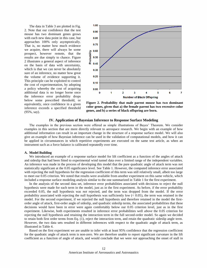
The data in Table 3 are plotted in Fig.

2. Note that our confidence that the test

mouse has two dominant genes grows

with each new data point in this case, but

approaches 100% only asymptotically.

That is, no matter how much evidence

we acquire, there will always be some

prospect, however remote, that the

results are due simply to chance. Figure

2 illustrates a general aspect of inference

on the basis of data with uncertainty,

which is that we can never be absolutely

sure of an inference, no matter how great

the volume of evidence supporting it.

This principle can be exploited to control

the cost of experimentation, by adopting

a policy whereby the cost of acquiring

additional data is no longer borne once

the inference error probability drops

below some prescribed threshold, or

equivalently, once confidence in a given

inference exceeds a specified threshold

(95%, say).

IV. Application of Bayesian Inference to Response Surface Modeling

The examples in the previous section were offered as simple illustrations of Bayes’ Theorem. We consider

examples in this section that are more directly relevant to aerospace research. We begin with an example of how

additional information can result in an important change in the structure of a response surface model. We will also

give an example of how Bayesian inference can be used in the validation of computational models, and how it can

be applied in circumstances in which repetitive experiments are executed on the same test article, as when an

instrument such as a force balance is calibrated repeatedly over time.

A. Model Building

We introduced an example of a response surface model for lift coefficient as a function of the angles of attack

and sideslip that had been fitted to experimental wind tunnel data over a limited range of the independent variables.

An inference was made in the process of developing this model that the pure quadratic angle of attack term was not

statistically significant at the 0.05 significance level. See Table 1. However, the computed inference error associated

with rejecting the null hypothesis for the regression coefficient of this term was still relatively small, albeit too large

to meet our 0.05 criterion. We noted that results were available from another experiment on this same vehicle, which

included a response surface modeling analysis similar to the one summarized in Table 1 for the first experiment.

In the analysis of the second data set, inference error probabilities associated with decisions to reject the null

hypothesis were made for each term in the model, just as in the first experiment. As before, if the error probability

exceeded 0.05, the null hypothesis was not rejected, and the term was dropped from the model. If the error

probability associated with rejecting the null hypothesis was sufficiently low (< 0.05), the term was retained in the

model. For the second experiment, if we rejected the null hypothesis and therefore retained in the model the first-

order angle of attack, first-order angle of sideslip, and quadratic sideslip terms, the associated probabilities that these

decisions would have been in error were again comfortably below our 0.05 criterion level, just as in the first

experiment. Likewise, both experiments resulted in inference error probabilities well above the 0.05 criterion for

rejecting the null hypothesis and retaining the interaction term in the full second-order model. So again we decided

to retain both first order terms from Eq. (1), reject the interaction term, and retain the quadratic sideslip angle term.

However, the two data sets resulted in different inferences with respect to the quadratic angle of attack term, as

illustrated in Table 4.

Based on the first experiment we are unable to infer with at least 95% confidence that the regression coefficient

for the quadratic angle of attack term is non-zero. We are therefore unable to report significant curvature in the lift

coefficient as a function of angle of attack, and would conclude that we were not approaching the onset of stall in

Figure 2. Probability that male parent mouse has two dominant

color genes, given that a) the female parent has two recessive color

genes, and b) a series of black offspring are born.


13

the angle of attack range examined in this experiment. We reach precisely the opposite conclusion from an analysis

of the second experiment. A Bayesian analysis allows us to reconcile these results in such a way that proper weight

is given to both experiments.

Let us assume that our two estimates of the regression coefficient are random variables based on normally

distributed data samples with means 1 and 2 and standard deviations 1 and 2, where the subscripts identify the

two experiments. It is the convention to refer to one of these as the prior distribution and to say that it is revised by

information from the other experiment. However, this does not imply any time-ordering. That is, the ―prior‖

distribution does not have to have been established first. It is equally valid to say that conclusions based on results

obtained in either experiment are revised because of information from the other one. However, we will arbitrarily

declare the results displayed in Table 1 as having come from the prior distribution, which we will revise based on

the additional results for the quadratic angle of attack term that are displayed in the right column of Table 4.

It can be shown9–11

that the posterior distribution in such a case is also normally distributed, with a mean, 0, and

a standard deviation, 0, represented as weighted combinations of the means and standard deviations of the two

experimental data samples:

0 1 1 2 2

1 2

1w w

w w

(16a)

1 22

0

1w w

(16b)

Where the weighting functions, wi, are

1 22 2

1 2

1 1 and w w

(16c)

The mean of the posterior distribution for the regression coefficient is just a weighted average of the regression

coefficient estimates from the two experiments, with the weighting determined by the uncertainty in each estimate.

In this way, the greater weight is given to the estimate with the least uncertainty. The variance of the posterior

distribution for the regression coefficient is based on a pooling of the variances from each experiment.

Table 4. Selected Characteristics of Quadratic Angle of Attack Term in Second-Order Response

Surface Model of Lift Coefficient as a Function of the Angles of Attack and Sideslip.

Characteristics of Quadratic Angle

of Attack Term First Experiment, Table 1 Second Experiment

Regression Coefficient -1.051E-03 -1.190E-03

Std Err in Coefficient 5.48E-04 4,90E-04

Coefficient as Multiple of Std Err 1.92 2.43

Inference Error Probability if Term

Retained 0.0842 0.0076

Max acceptable Inference Error

Probability 0.0500 0.0500

Inference Reject Term (Err prob > 0.05) Retain Term (Err prob <0.05)


14

After inserting numbers from Table 4 into Eqs. (16), we conclude that the posterior estimate of the regression

coefficient for the quadratic angle of attack term in our lift coefficient model has a value of

3 33

0 2 24 4

2 24 4

1 1.051 10 1.190 101.128 10

1 1 5.48 10 4.90 10

5.48 10 4.90 10

x xx

x x

x x

(17a)

with a standard deviation of

4

0

2 24 4

13.653 10

1 1

5.48 10 4.90 10

x

x x

(17b)

Figure 3 compares three normal distributions for the quadratic angle of attack regression coefficient. The black

one is the prior distribution, the red one represents the new data, and the blue one is the posterior distribution,

reflecting a Bayesian revision of the prior distribution per Eqs. (16) to reflect the information in the new data. (This

figure displays positive means for the distributions consistency with Eq. (3), although the actual quadratic angle of

attack regression coefficient is negative—concave down.)

By inserting values from Eqs. (17) into Eq. (3), the inference error probability associated with rejecting the null

hypothesis for the posterior (revised) distribution is computed as 0.0010, down from the 0.0842 value associated

with the prior distribution. That is, the original odds against an inference error if we retained the quadratic angle of

attack term were about 11 to 1, or 1 chance in 12 of an erroneous inference. We had established our maximum

acceptable odds at 19 to 1, or 1 chance in 20 of an inference error. After taking into account the new data, if we infer

that the quadratic angle of attack term should be retained in the response surface model, the odds against that

inference being wrong increase dramatically, from 11:1 to 999:1, or only 1 chance in a thousand of an inference

error, well within our risk tolerance.

We are willing to assume that much

risk in rejecting the null hypothesis for

the quadratic angle of attack regression

coefficient, and we therefore retain it

in the model, concluding that the onset

of stall is in fact evident over the range

of angle of attack that we examined.

By incorporating additional

information that allowed us to revise

our prior conclusion about the

significance of the quadratic angle of

attack term, we achieved a substantial

reduction in inference error risk. This

was due in part to the fact that the

signal to noise ratio for the second data

set was greater than the first. The

estimated regression coefficient was

further from zero and the standard

deviation in estimating the regression

coefficient was less in the second data

set than in the first.

The revised coefficient estimate is

a weighted average of the coefficient

estimated from each of the two data

Figure 3. Probability distributions for quadratic angle of attack

regression coefficient. Area under the curve to the left of zero

represents the error probability for rejecting the null hypothesis. It

exceeds 0.05 for the prior distribution (black) but not for the yellow

(posterior) distribution, revised to account for new data (red).


15

sets, and so it lies between the two individual estimates. However, it is still further from zero than in the prior

experiment.

The prior variance was pooled with new data featuring less variance, which suggests that the revised variance

would be smaller on that account. It is in fact a general result that pooling the variance associated with two samples

results in less variance than either component sample. This can be seen clearly by combining Eqs. (16b) and (16c) as

follows:

2 2 2 221 2 1 202 2 2 2 2 2 2

0 1 2 1 2 1 2

1 1 1

(18)

It follows immediately that

22 210 12

1 21

(19a)

and

22 220 22

2 11

(19b)

The combination of a narrower probability distribution and a shift in the mean away from zero resulted in a

greater signal to noise ratio and therefore a reduction in the probability of an improper inference associated with the

conclusion that the regression coefficient was in fact non-zero. Figure 4 displays the regression coefficients for the

prior and revised distributions as well as for the added data used to revise the prior. They are represented in this

figure as multiples of the standard error in estimating them. There is a transparent colored box in Fig. 4 covering the

range from minus two to plus two standard deviations. Coefficients lying within this box are too close to zero to be

declared non-zero with at least 95%

confidence, as our risk tolerance

specification requires. Coefficients

outside this box can be distinguished

from zero with acceptable inference

error risk.

Note that the original coefficient

estimate was just inside the box,

reflecting the ~0.08 inference error

probability from Table 1 that just did

exceed our 0.05 tolerance level. The

regression coefficient for the new

data is comfortably outside the ±2

range and the revised regression

coefficient, with a substantially

smaller standard deviation, is a

sufficient number of standard

deviations away from zero that we

incur relatively little risk by inferring

that this coefficient is indeed real

(non-zero) and therefore belongs in

the model.

Even though the quadratic angle

of attack term was the only one in

doubt, we apply the Bayesian

revision process captured in Eq. (16)

Figure 4. Quadratic angle of attack regression coefficient in

multiples of standard deviation. Magnitude must be greater than 2

(positive or negative) to be resolvable from zero with at least 95%

confidence. Original (prior) estimate was just inside the limit.

Estimate from new data was resolvable as was revised estimate.


16

to each of the coefficients in the model to generate a revised model that reflects all the information in both data sets.

We noted above that residuals from the model in Eq. (6) , in which the quadratic angle of attack term is missing, had

an average magnitude of 0.0013, which exceeded our error budget of 0.0010 in this test by 30%. We use the revised

model in Eq. (20) to predict lift measurements for the same 16 combinations of angle of attack and angle of sideslip

as before.

2 2

0 1 1 2 2 11 1 22 2y b b x b x b x b x (20)

The revised model, Eq. (20), resulted in residuals with an average magnitude of 0.0008, well within the error

budget of 0.0010, and reflecting a 38% reduction in prediction error relative to the initial model. Figure 5 compares

the residuals of the prior and revised model with the error budget.

B. Validation of Computational Models

It is not uncommon for different computational codes to produce different results, notwithstanding the fact that

they were developed to describe a common phenomenon.12

One might say that to at least some extent, this is the

norm.13

When multiple computational codes are evaluated, their predictions might be compared with some

reference to determine how great a difference there is between the prediction of each code and that reference. The

reference could be a measurement of the physical phenomenon which the codes seek to predict, or absent any

suitable physical measurement to serve as a standard, it might simply be the mean of all code predictions.

Consider a case in which, for simplicity, we assume that there are only two different computational codes, and

that the validity of each is to be assessed by comparing predictions with a physical measurement. There will

obviously be uncertainty in the physical measurement used as a reference, in the form of ordinary experimental

error. Each code will also have uncertainty, notwithstanding the absence of variance in replicated computations.† As

a general rule, the degree of uncertainty in a code prediction depends on the combination of independent variable

levels for which the prediction is made. There are several reasons for this, including the fact that the slope of the

response function will generally vary over the design space, resulting in a greater or lesser impact of uncertainties in

the independent variable settings.

For the purpose of this example, we assume that each code is intended to quantify drag on a specified test

aircraft, and that its ability to do so will be evaluated by comparing code predictions with flight data acquired at a

certain set of conditions. We assume further that the uncertainty in flight measurements has been quantified through

an appropriate analysis of test data, and

that the uncertainty associated with

predictions made by each computational

code has been estimated.

Let us say that flight conditions are

chosen for this comparison such that the

empirically determined drag is 700 counts

with a standard deviation of 30 counts.

The first code estimates the drag to be 750

counts for these same conditions, with a

standard error of 10 counts. The second

code estimates the drag for these

conditions to be 650 counts, but it is only

capable of rather less precise estimates,

characterized by a standard error of 60

counts.

At first glance it might seem as if both

codes performed comparably in that they

each produced predictions that differed

from the measured flight data by identical

amounts—50 counts. However, the simple

† The fact that a computational code will produce the same numerical result without variance for any number of

replicates does not suggest that there is no uncertainty in a given code prediction. It simply implies that the

uncertainty in a computational code cannot be quantified by replication.

Figure 5. Residuals from the prior response surface model

exceeded the error budget. Bayesian inference justified the

addition of an additional term to the model that resulted in

residuals that were within tolerance.


17

comparison is potentially misleading for two

reasons. First, both of the computational

estimates as well as the measured drag are

random variables, describable in terms of

probability distributions that are characterized

by dispersion metrics as well as location metrics.

Comparing each code prediction with the

experimental data only on the basis of their

location metrics (means of their probability

distributions) fails to account for the dispersion

(variance) in each estimate. Furthermore, the

measured drag is itself no more than an estimate,

subject to uncertainty just as the computational

estimates are. The assumption that the measured

estimate should be given more weight than the

computational estimates is only valid if the

uncertainty in the measured estimate is

significantly less than the uncertainty in either

computed value. That is not true in this case, and

in fact the standard deviation for Code 1 is even

smaller than the standard deviation for this

particular sample of flight data.

In using the measured data to assess the

computational results, we should ask how much

the sponsor of each code is able to learn by an

exposure to the measured results. We can use

Bayesian revision to address this question. We

have the mean and standard deviation of each

code’s distribution prior to the data, and the

mean and standard deviation of the data. We can

therefore use Eqs. (16) to compute the posterior

distributions when each code’s prior distribution

is revised by the information in the data. Means

and standard deviations for the prior and

posterior code distributions are listed in Table 5.

Figure 6 compares these distributions.

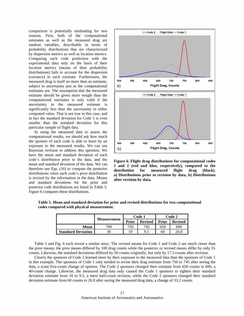
Table 5 and Fig. 6 each reveal a similar story. The revised means for Code 1 and Code 2 are much closer than

the prior means; the prior means differed by 100 drag counts while the posterior or revised means differ by only 55

counts. Likewise, the standard deviations differed by 50 counts originally, but only by 17.3 counts after revision.

Clearly the sponsors of Code 2 learned more by their exposure to the measured data than the sponsors of Code 1

in this example. The sponsors of Code 1 only needed to revise their drag estimate from 750 to 745 after seeing the

data, a scant five-count change of opinion. The Code 2 sponsors changed their estimate from 650 counts to 690, a

40-count change. Likewise, the measured drag data only caused the Code 1 sponsors to tighten their standard

deviation estimate from 10 to 9.5, a mere half-count revision, while the Code 2 sponsors changed their standard

deviation estimate from 60 counts to 26.8 after seeing the measured drag data, a change of 33.2 counts.

Table 5. Mean and standard deviation for prior and revised distributions for two computational

codes compared with physical measurement.

Measurement

Code 1 Code 2

Prior Revised Prior Revised

Mean 700 750 745 650 690

Standard Deviation 30 10 9.5 60 26.8

Figure 6. Flight drag distributions for computational codes

1 and 2 (red and blue, respectively), compared to the

distribution for measured flight drag (black).

a) Distributions prior to revision by data, b) Distributions

after revision by data.


18

Note how differently we regard the two computational codes after this type of comparative analysis. Originally

we were willing to conclude that little distinguished one code from the other, in that they each predicted the

measured drag with the same error. After accounting for the relative uncertainty in each code prediction (and in the

confirming measurement!), we see that conclusions based on one of the codes would be altered substantially more

by the experimental observations than the other.

The reason is that the uncertainty in drag estimates made by one of the codes was substantially greater than the

other code; users of one code would have only a relatively vague idea of the drag they were estimating, while users

of the other code would have a rather more precise estimate. In fact, in this example the users of Code 2 had less

uncertainty in their estimates than the experimentalists providing the confirmatory measurement, while explains why

their posterior knowledge was revised so little as a result of their exposure to this additional information. On the

other hand, users of Code 1 began with a relatively imprecise prediction of the measured drag, and their estimates

were subject to rather greater revision as a result of the measurement.

We can see this situation graphically in Fig. 6a, where the prior distribution for Code 2 is considerably more

peaked than the prior distribution for Code 1, and it is even rather more peaked than the distribution for the physical

measurement. For this reason the data has rather little influence on the revised distribution of Code 1, while it has a

fairly dramatic influence on the revised distribution of Code 2, as seen in Fig. 6b.

We noted above an alternative for evaluating individual computational codes when there is no physical

measurement available to serve as a reference against which to make comparisons. It is a customary assumption that

when multiple estimates of some phenomenon are available, the median or the mean of those estimates is a more

reliable estimator than any one individual estimate. It is likewise customary to regard estimates that are the farthest

from this reference to be the least reliable (―outliers,‖ if they are sufficiently far away). This suggests that some

appropriately weighted combination of computational code predictions might serve as a suitable reference against

which to measure individual predictions. At the very least, the variance in an ensemble of computational code

estimates can be regarded as an indicator of the state of the art for computational predictions.14

Bayesian methods summarized in this paper are well suited for generating a weighted reference prediction

against which to compare individual codes. Eqs. (16) suggest that a rational weighting could be based on the

uncertainty associated with each individual code, with those codes featuring the least uncertainty weighted the most

and those featuring the greatest uncertainty weighted the least.

It is beyond the scope of this paper to consider explicit methods for estimating the uncertainty of individual

computational codes, except to say that this is an area of increasing interest in the computational aerospace

community. The author has offered some ideas at what at this writing has been the most recent conference devoted

exclusively to this topic,15

and the literature of computational uncertainty continues to grow. For purposes of

illustration, we assume that some rational means exists by which to assign uncertainty to the response predictions

made by each computational code. Also for illustration, we assume that three computational codes have produced

estimates for flight drag for identical flight conditions. We will use for illustration the same estimates reported in

Table 5 for Codes 1 and 2, and assume now that the physical measurement reported in that table describes the prior

distribution for a third computational code. Equations 16 extend naturally to multiple distributions. For prior means

of 650, 700, and 750, with corresponding standard deviations of 60, 30, and 10, these equations result in a mean

weighted by the reciprocal of variance in each estimate of 742.7, with a pooled standard deviation of 9.4. These

calculations are summarized in Table 6.

Table 6. Comparison of three codes with and without accounting for uncertainty in predictions.

Code 1 Code 2 Code 3

Mean 750 650 700

Standard Deviation, 10 60 30

Residual

Weighting

by 1/2

750-742.7=7.3 650-742.7=-92.7 700-742.7=-42.7

No

Weighting 750-700=50 650-700=-50 700-700=0

Ranking

Weighting

by 1/2

1 3 2

No

Weighting 2 2 1


19

Note how differently the code predictions are ranked if the reference is computed by weighting each prediction

by the information it contains, as quantified by the reciprocal of the variance in each estimate. With no weighting,

Code 3 has the highest ranking by virtue of the fact that its prediction lies squarely in the center of this three-point

sample. Codes 1 and 2 tie for second place and are regarded as indistinguishable since their predicted responses are

equally displaced from the sample median.

However, when a weighted mean is constructed that accounts for the uncertainty in each prediction, an entirely

different picture emerges. Now Code 1 is regarded as having made the most reliable prediction, based on its

relatively small variance (or equivalently, the relatively large amount of information contained in its estimate). Code

2, regarded as equivalent to Code 1 when prediction uncertainty was ignored, is now ranked in third place, again

because its relatively large variance translates into only rather vague predictions of flight drag for the combination of

independent variables considered in this comparison. Code 3, ranked #1 when prediction uncertainty was ignored, is

now in second place behind Code 1 because its variance is three times larger than that of Code 1.

Obviously the utility of a Bayesian approach to computational code evaluation depends critically on the quality

of uncertainty estimates in the individual code predictions. This argues for continued attention to the problem of

assessing computational uncertainty.

C. Instrumentation Calibration

We consider as our last example of the application of Bayesian inference to response surface methods a special

case in which an experiment is replicated on the same test article. This situation arises from time to time in different

contexts, but it is the norm for experiments designed to calibrate measurement systems or individual instruments.

The same experiment is typically executed each time an instrument is calibrated. To serve as a specific and common

example, we will consider a force balance that is calibrated repeatedly over time.

It is customary in a force balance calibration experiment to consider only the latest calibration results in defining

the coefficients of the transfer function that relates the balance’s electrical output to the applied forces and moments.

Notwithstanding the fact that this same balance may have been calibrated on many previous occasions, the results of

those prior calibrations are seldom taken into account except for occasional comparisons to determine the general

level of agreement with the most recent calibration. Since earlier calibration results will have been obtained with

considerable expense and effort, it seems wasteful to simply discard all of that prior information each time the

instrument is calibrated anew.

Bayesian inference models human learning by providing a mechanism for revising prior knowledge to reflect

new information. In the context of a calibration experiment, this implies that information obtained in prior

calibrations need not be lost each time an instrument is recalibrated. The calibration experiment can be regarded as

an opportunity to obtain additional information that can be used to revise prior calibration results.

Force balances are calibrated by applying a prescribed schedule of loads and recording the corresponding

electrical outputs. These data are typically fitted to a calibration model using linear regression. This model can be

used to predict electrical outputs as a function of loads, and is typically inverted to enable the specification of

applied loads for a given combination of electrical outputs recorded in a wind tunnel test, say.

There are different force balance designs in use but a common balance configuration measures three components

of force (normal, axial, and side force with respect to a specified coordinate system), and three moment components

(pitching moment about the side force axis, rolling moment about the axial force axis, and yawing moment about the

normal force axis). Force balances are designed with the goal of producing a linear instrument capable of

independent force and moment measurements. If that idealized goal could be achieved, then a simple first-order

polynomial in six independent variables would be adequate to describe the relationship between any combination of

forces and moments experienced by the balance and the electrical output produced for each force and moment

component.

0 1 1 2 2 3 3 4 4 5 5 6 6y b b x b x b x b x b x b x (21)

where y is the electrical output for any one of the six forces and moments (often some combination of strain gage

outputs), the bi are regression coefficients, and the xi are applied loads.

Unfortunately, a perfectly linear force balance with totally independent measures of the forces and moments is a

mathematical abstraction that has proven elusive to engineer in practice. Typically there are some small interactions

across the channels of a real force balance—the sensitivity or change in electrical output as one force or moment

changes typically depends on the levels of other forces and moments that are simultaneously applied, for example.

In addition to such interactions, there is generally some pure non-linearity (interactions of loads with themselves).


20

For example, the change in electrical output corresponding to a unit change in applied load if often different for low

loads than high loads. The electrical output is in such cases is a second-order (or higher) function of applied pure

loads. The end result of this interactive and non-linear behavior is that a rather more complex calibration model is

needed than the one described in Eq. (21).

For a single-piece six-component force balance, a second-order response model in six independent variables has

been traditionally fitted in the calibration process, requiring 15 interaction terms and six pure quadratic terms in

addition to the seven terms in Eq. (21), for a total of 28 terms in the model. Recent studies have indicated that third-

order terms may improve the balance calibrations, which imply up to 84 mathematically possible candidate terms in

the calibration equation for a six-component single-piece balance. In actual practice, most of these terms are either

non-existent (terms that correspond to an interaction that does not occur naturally in a given balance, for example),

or so small that the additional uncertainty they contribute to the calibration model exceeds their influence on model

predictions. In either case, retaining such terms would reduce the overall signal to noise ratio of the calibration.

Ulbrich and Volden at NASA Ames Research Center have pioneered the development of new methods and

software tools to identify and eliminate negligible terms from potentially large balance calibration models, resulting

in compact math models and improved balance calibrations.16-20

Parker, et. al.,21-25

DeLoach and Philipsen,26

and

Philipsen and Zhai27

have examined the use of specialized balance calibration hardware and the design of compact

balance calibration experiments facilitated by such hardware that are scaled for reduced calibration models.

A balance calibration experiment has in common with all response surface modeling experiments a process in

which decisions are made to reject or retain candidate terms in a proposed model. This process was illustrated with

the first example in this section of the paper, in which null hypotheses are established for each candidate term, and

an inference is made as to whether that hypothesis should or should not be rejected. Each inference has a non-zero

probability of being in error, which can be estimated and which is compared with a prescribed maximum acceptable

inference error probability. Terms are rejected or retained in the model based on how the associated inference error

probability compares with what is deemed acceptable. A consensus is reached and documented with respect to

acceptable levels of inference error risk early in the formal experiment design process.

It is possible to apply Bayesian inference methods outlined in this paper by using current calibration results to

revise prior inference error probabilities associated with each term in the calibration model. In this way we can

modify what we already know about the model with information recently obtained. The pooling of variances that

occurs with each new calibration results in progressively higher precision inferences with respect to decisions to

retain or reject terms from the model. Note that retention decisions are generally unambiguous (vanishingly small

inference error probabilities) for the first-order terms in a balance calibration model, and can also be quite clear for

the relatively strong interaction terms. However, for numerous model terms with smaller regression coefficients, the

decision to retain or reject that term can turn on the level of unexplained variance in the calibration data or other

subtle effects. It is possible that such terms might be retained in one calibration and rejected in another.

This circumstance gives rise to an interesting model selection opportunity. Imagine a series of calibrations that

have been performed on the same balance. The first-order terms and larger interaction terms will have been retained

in the response model for every calibration with negligible inference error probability, however some of the terms

with smaller regression coefficients may be retained in some calibrations and rejected in others. That is, as a result

of the most recent calibration data, one might decide to include a term that was previously rejected or reject a term

that was previously retained in the model. This gives rise to the notion of transitions from one calibration to another

between one state in which a given term is retained in the model, and another state in which it is rejected.

Over a sufficient number of calibrations, one could begin to estimate conditional transition probabilities. If we

let the subscripts ―0‖ and ―1‖ refer to states in which a given term is missing or present in the model, respectively,

we can define p00 as the probability that a term that was rejected from the model in the last calibration would be also

rejected in the current calibration, and p01 would represent the probability that a term rejected the last time would be

retained this time. (Obviously, these two probabilities sum to 1.) Likewise, p10 represents the probability that a term

retained in the prior calibration would be rejected in the current one, and p11 represents the probability that a given

term is retained in two consecutive calibrations. These latter two probabilities also sum to 1.

Let us now define 0 and 1 as elements of a 1 × 2 column vector, , describing the proportion of times that a

given term has been rejected or retained. We assign the four transition probabilities to elements of a transition

probability matrix, P, as follows:

00 10

01 11

p p

p p

P (22)


21

We then have=Pi=i+1 which expands as follows:

00 0, 10 1, 0, 1i i ip p (23a)

01 0, 11 1, 1, 1i i ip p (23b)

Equation (23a) simply states that the fraction of the total number of calibrations in which a given term was

inferred to be in state ―0‖ (rejected) is, after the (i+1)st calibration, equals the fraction that were in that state after the

ith

calibration and stayed in that state, plus the fraction that were in state ―1‖ (retained) after the ith

calibration that

were then rejected in the (i+1)st calibration. Equation (23b) similarly describes the proportion in state ―1‖ (retained)

after the (i+1)st calibration as the sum of those starting in state ―0‖ and transitioning to state ―1‖ plus those starting in

state ―1‖ and staying there.

We have described a series of discreet events (calibrations) in which the state of a given term in the calibration

model after each calibration (retained or rejected) is a random variable (i.e., not deterministic but defined by some

probability). This chain of events has what is known as the ―Markov property,‖ in that given the state transition

probability matrix, Eq. (22), the state of each term in the calibration model depends only on the state of that term

after the last calibration. Such a process is known mathematically as a Markov chain.

Markov chains have certain properties that we can exploit in this analysis. Specifically, given Eqs. (23), the

vector is an equilibrium distribution if its elements πj sum to 1. That is certainly the case for this Markov chain;

the probability that a given term in the model will either be retained or rejected after each calibration is always 1.

The fact that the vector is therefore an equilibrium distribution means that the percentage of times a given term

will be rejected (or retained) approaches a constant after a sufficient number of calibrations. That constant depends

only on the transition probability matrix, P, so the system converges to a final equilibrium state distribution that is

completely independent of the starting distribution.

We can compute the equilibrium state distribution for each term (i.e., the long-term probability that the term will

be retained or rejected) by noting that at equilibrium, i=i+1, so that Eqs. (23) become:

00 0 10 1 0p p (24a)

01 0 11 1 1p p (24b)

Combining this with the fact that 0 + 1 = 1, yields the following formulas for the equilibrium state distribution

probabilities 0 and 1:

100

01 10

p

p p

(25a)

011

01 10

p

p p

(25b)

We can examine certain special cases. If p10 = 0 (no instances in which a term that appears in the model is ever

rejected in a subsequent calibration), then 0 = 0, 1 = 1, and the probability is 100% that this term will be in the

calibration model. If p01 = 0 (no instances in which a rejected term ever appears in the model in a subsequent

calibration), then 0 = 1 and 1 = 0, so the long-term probability that this term will ever appear in the calibration

model is zero. If p10 and p01 are such that 0 represents an acceptably low probability of an inference error for a


22

given term, then the decision to retain that term can be made for all subsequent calibrations of this balance. If p’

represents that critical probability, we have the following condition for 0:

100 10 01 10

01 10

pp p p p p

p p

(26)

or

0 01 10

1 pp p p

p

(27)

Equation (27) informs us that if, for example, p’ = 0.05 as is a common convention, then we must have

p01 ≥ 19p10 as a condition for retaining the term. That is, we incur less than a 5% probability of an inference error if

we retain a term for which the long-term 0-to-1state transition probability is at least 19 times greater than the long-

term 1-to-0 state transition probability. Such probabilities are revealed through a series of calibrations, with prior

calibrations contributing equally to the model selection process.

In general, we expect that consistent calibration methods will result in relatively large or relatively small values

of p01 and p10. That is, we do not expect terms to be equally likely to be retained in one calibration and rejected in

another if the calibration process is consistent. This is only likely to occur when the magnitude of the regression

coefficient is on the order of the uncertainty in estimating it, so that slight variations in the unexplained variance

from calibration to calibration are sufficient to either mask the term or to marginally reveal it. In such circumstances

we would tend to discard the term on the grounds that such small regression coefficients are not likely to make a

practical difference in response model predictions, while each retained term carries with it some incremental

contribution to the total prediction variance, per Eq. (2). That is, when in doubt we yield to a prejudice in favor of

rejecting terms rather than retaining them.

V. Discussion

Bayesian inference is especially relevant to response surface modeling experiments such as wind tunnel tests

because of the critical role that reference distributions and formal hypothesis testing play in the construction of

response surface models. We represent an unknown response function as a Taylor series which for mild and

commonly occurring conditions is an exact representation provided we retain an infinite number of terms. Resource

constraints prevent the acquisition of sufficient data to fit an infinite number of terms, and in any event such

extravagance is not necessary in practical circumstances. We are, however, always faced with the problem of

inferring which terms to reject and which to retain. We make objective retention/rejection decisions by noting the

location of a regression coefficient estimate relative to a reference distribution with a mean of zero and a standard

deviation reflecting the uncertainty in estimating the coefficient. If the coefficient estimate is located a sufficient

number of standard deviations away from zero, we retain that term in the model. Otherwise, we reject it.

Bayesian inference facilitates ―learning by experience‖ in that it permits prior knowledge to be revised by

additional information. The role that such prior information plays has been a source of controversy historically, with

critics of the Bayesian approach noting that reliance upon prior information in some sense diminishes what the

current data ―is telling us.‖ Bayes himself recognized this potential criticism, and suggested in what came to be

known as Bayes’ Postulate that such objections could be overcome by assuming a uniform prior distribution in

circumstances for which little is known a priori. He apparently was sufficiently unsure of this point that he did not

publish it, however. Bayes’ views only came to light when his work was published after his death by his friend,

Richard Price28

.

Advocates of Bayes’ methods note that his basic theorem (Eq. (9), restated as Eq. (13)) is a straightforward

statement of conditional probability and is not in and of itself in dispute. It is rendered controversial by

considerations of the role that the prior distribution plays as noted above, and also by fundamental notions of the

meaning of probability. The conventional (or ―frequentist‖) view of probability is that it is related to the frequency

with which events can be expected to occur. Bayesians adopt a more liberal interpretation, associating probability

with the extent to which a given viewpoint is held. A Bayesian would assign a high probability of occurrence to an

event he felt was likely to occur, for example. This leads to the notion of subjective prior distributions, a significant

point of contention among frequentists who argue that posterior means can be influenced to take on virtually any


23

value by a suitably selected subjective prior. This renders statistical inference, they claim, much too vulnerable to a-

priori prejudices. On the other hand, Bayesians point to circumstances in which suitable frequency-based probability

information is unavailable and yet inferences must be made, in which case good-faith subjective probability

estimates based on experience have a role to play. Examples include inferences with respect to rare disasters such as

aircraft accidents or nuclear power plant failures, or other decision-making circumstances in which limited prior

information is available, such as whether to drill for oil at a given location. In such cases, an informed but

nonetheless subjective evaluation may constitute much of what is believed to be true before the introduction of what

might in fact be rather meager additional evidence.

Box and Tiao29

enumerate and systematically address issues surrounding the prior distribution, and develop a

practical variation of Bayes’ Postulate involving locally uniform prior distributions. It was noted above in the

discussion of Fig. 6 that the relative influence of the prior distribution and the additional data used to revise it

depends on the ―peakiness‖ of the probability distributions. For circumstances in which the precision of the new

information is significantly greater than that of the prior information, the new information will dominate the prior in

defining the posterior distribution. For practical circumstances in scientific inquiry this is generally the case, as

investigations are seldom undertaken absent the prospects of some resulting increase in knowledge, which implies a

dominant role for the new information and a less influential role for the prior distribution. (In short, if we ―knew‖

the answer a priori, we would not have undertaken the experiment.) For the response surface modeling applications

considered in this paper, there is even less of a controversy. The prior distributions considered in such applications

involve an interpretation of probability that is generally consistent with conventional frequentist notions.

Bayesian inference is appealing for scientific research because it is based on a distinction between what is true in

nature, and what is inferred. The cruise lift of a new aircraft may or may not in fact exceed some minimum

certification requirement. But in either case we might have to make an inference about whether it does or does not

based on observations we have made of a model airplane set to emulate cruise conditions in a wind tunnel. It is

possible for the results of a wind tunnel test to suggest that the lift is adequate when it is in fact adequate, but it is

also possible that the results will suggest the lift is adequate when it is not. Bayesian inference provides a

mechanism for explicitly recognizing such limitations of experimentation. When we use Bayesian inference to

evaluate the probability that ―A‖ is true given that we have observed ―B,‖ we not only consider the probability of

observing ―B‖ when ―A‖ is true, but also the probability of observing ―B‖ when ―A‖ is not true. See Eq. (13). That

is, we are forced to take into account the fact that our measurements are imperfect, and that it is possible to obtain an

indication that something is true both when it is true and when it is not true.

To illustrate this important point, consider an example drawn from the news just prior to the conference in which

this paper is presented. In December of 2007, a report was presented to the commissioner of major league baseball,

Mr. Bud Selig, on the use of steroids among professional baseball players. The report was accompanied by

significant publicity, and amounted to a severe indictment of the sport and many of its key players.

The author downloaded the full report and performed keyword searches on such seemingly relevant words as

―accuracy‖ and ―precision‖ to gain some insight into the reliability of the tests used to detect steroids. The word

―accuracy‖ appears exactly once in the 311-page report (in a commentary about an eyewitness report) and the word

―precision‖ does not appear at all. Similar searches for such strings as ―inference,‖ ―false positives,‖ and ―false

negatives‖ returned no hits. On the other hand, a Web search revealed a site apparently devoted to the topic of

steroids in baseball that listed the names of 12 players who had experienced the league’s 10-day suspension rule for

first-time offenses, a number nominally consistent with the Commissioner’s assertion that 1.2% of the players had

used steroids last season, based on a combined American League and National League roster of 854 players.

We will augment this meager information with what are believed to be reasonable suppositions to illustrate how

a Bayesian analysis might be performed on the steroids-in-baseball scandal. (The central points of this illustration

are not dependent on the suppositions.)

Let us assume that a steroid test is ―95% accurate,‖ by which it is meant that if a player who uses steroids is

subjected to this test, he will test positive 95% of the time. This means that 5% of steroid users will pass this test.

Let us also assume that the test will exonerate non-users 95% of the time, which nonetheless means that 5% of those

who do not use steroids will be falsely accused.

If we use for this illustration the figure cited above by the Commissioner of 1.2% as representative of the

fraction of players who actually do use steroids, we can easily compute how many users and non-users will test

positive. We assume that 0.012 of the league uses steroids and 0.95 of those will test positive, so 0.012 × 0.95 =

0.0114 of the league will be users who test positive. On the other hand, 1 – 0.012 = 0.988 is the fraction of the

league that is clean in this example, of which 0.05 will wrongly test positive. So 0.988 × 0.05 = 0.0494 is the

fraction of the league that will be falsely accused. We will have 0.0114 + 0.0494 = 0.0608 as the total fraction of the

league that will test positive (roughly 52 players), of which only 0.0114 × 854, or about 10, will actually be steroid


24

users. Therefore, the probability that a player actually does use steroids, given that he has tested positive, is only

about 10 in 54, or roughly 18.5%.

The probabilities of false negatives and false positives were estimated in this example for the sake of illustration,

although they are believed to be not unrealistic. The total number of positive tests computed in this example—52—

is consistent with numbers reported in the media for active players said to have tested positive for steroid use.

The calculations presented in this example were rounded to ensure an integer number in each category of

accused players (correctly accused and falsely accused). An exact calculation would invoke Eq. (13), with ―A‖

corresponding to a player actually being a steroid user and ―B‖ corresponding to a positive test. In this example we

would have

0.012

| 0.95

| 0.05

1 0.012 0.988

| 0.95 0.012| 0.1875

0.95 0.012 0.05 0.988| |

P A

P B A

P B A

P A

P B A P AP A B

P B A P A P B A P A

as the exact solution, which compares with our 18.5% approximation.

These results illustrate how much difference there can be between what is true in nature, and what is inferred in a

test. There is only an 18.75% probability that a player who tests positive with this test will actually be a steroid user,

notwithstanding the ―95% reliability‖ of the test. This is an example of how inferences can be quite different when

measurement imperfections are explicitly taken into account, as they are when Bayesian inference is applied.

VI. Concluding Remarks

This paper has provided an elementary introduction to the subject of Bayesian inference as it might be applied to

experimental aerospace research in general, and experimental aeronautics in particular. Examples have been

provided to show the applicability of the method to response surface modeling, to the validation of computational

models, and to tasks which involve repeated experiments on the same test article, as in the calibration of an

instrument over time.

Bayesian inference extends insights available from a conventional frequentist perspective of statistics by

explicitly accounting for the inevitable limitations of any system or process used to observe nature. It assumes we

originally hold certain beliefs with some uncertainty, and that we try to perfect our knowledge by the introduction of

new information that is also imperfect. This method encompasses as a special case the common situation in

experimental research when we hold no particular beliefs a-priori; that is, when the probability associated with a

given inference is 0.5 before we have acquired any new information in the form of experimental data.

Bayesian inference has special practical utility in that it models the learning process that is fundamental to

scientific research, and that is an explicit element of the Modern Design of Experiments. We make progress in

MDOE through a series of cycles in which we alternately play the role of advocate and critic of a given proposition.

We advance a proposed model to describe nature in certain limiting circumstances, and then subject that model to

criticism that is often based upon the introduction of new information, itself imperfect. Throughout this process we

modify our original perceptions to account for the new information, rather than discarding them wholesale in

preference for a completely new set of suppositions based on the latest observations. We then subject our revised

models to criticism, and so on, until we are satisfied that they are adequate for a particular purpose. This provides a

mechanism of handing down information, often hard-won at great expense, from preceding cycles of investigation

through to future investigators.

The Modern Design of Experiments is based upon an intrinsically statistical framework in which a series of

inferences are made about the suitability of incorporating progressively higher-order terms in a series representation

of some system response, modeled as a function of specified independent variables. We make inferences for each

term in the proposed model by testing a null hypothesis that asserts a-priori that the term under evaluation is


25

insignificant and does not belong in the model. We only retain such a term if we are influenced by experimental

results to revise our initial view.

We may initiate such a process in a state in which we are completely neutral with respect to the question of

whether a given response model term should be retained or rejected; that is, in a state in which we assume that the

prior probability that the term is significant is 0.5—just as likely to be real as not. This attitude is often represented

as desirable in that it implies a laudable lack of prejudice with respect to the questions under investigation. And yet

it does not seem illegitimate to assume that a subject matter expert would have a priori knowledge that ought to be

taken into account. On the contrary, it seems unrealistic to assume otherwise. Bayesian inference provides a formal

mechanism for combining a priori knowledge with new observations to generate revised insights, giving proper

weight to the intrinsic uncertainty in what was originally believed and what has been newly learned.

The purpose of this paper has been simply to alert elements of the experimental aeronautics research community

to a framework for making progress that may be new to them, and which the author has himself only recently begun

to exploit. It is by no means a comprehensive tutorial on Bayesian inference, which is far too detailed a subject to

cover adequately in a single conference paper and with which the author claims no substantial experience. Yet there

seems to be a number of attractive elements to this approach to scientific inquiry, not the least of which from the

author’s perspective is its potential for seamless integration into the analytical methods of formal experiment design.

Readers are encouraged to make their own independent inquiries and evaluations of the utility of Bayesian inference

in experimental aeronautics research, but it is not unlikely that this topic will receive further attention as it becomes

more familiar to researchers in our field.

Acknowledgments

This work was supported by the Aeronautics Test Program of the National Aeronautics and Space

Administration.

References 1DeLoach, R., ―Applications of Modern Experiment Design to Wind Tunnel Testing at NASA Langley Research Center,‖

AIAA-98-0713, 36th AIAA Aerospace Sciences Meeting and Exhibit. Reno, NV, January 1998. 2DeLoach, R. ―Tailoring Wind Tunnel Data Volume Requirements Through the Formal Design Of Experiments,‖ AIAA-98-

2884, 20th Advanced Measurement and Ground Testing Conference. Albuquerque, NM. June 1998. 3DeLoach, R., ―Improved Quality in Aerospace Testing Through the Modern Design of Experiments (Invited),‖ AIAA 2000-

0825, 38th AIAA Aerospace Sciences Meeting and Exhibit. Reno, NV. January 2000. 4Box, G. E. P., and Draper, N., Response Surfaces, Mixtures, and Ridge Analyses, 2nd Ed., John Wiley and Sons, New York,

2007 5Montgomery, D. C., and Peck, E. A., Introduction to Linear Regression Analysis, 2nd Ed., John Wiley and Sons, New York,

1992. 6Myers, R. H., and Montgomery, D. C., Response Surface Methodology: Process and Product Optimization Using Designed

Experiments, Wiley Series in Probability and Statistics, 2nd Ed., John Wiley and Sons, New York, 2002. 7Draper, N. R., and Smith, H., Applied Regression Analysis, 3rd Ed., John Wiley and Sons, New York, 1998. 8Fisher, R. A., Statistical Methods and Scientific Inference, 2nd Ed., Oliver and Boyd, London, 1959. 9Berger, J. O. Statistical Decision Theory and Bayesian Analysis. 2nd Ed.. Springer Verlag, New York, 1999. 10Gelman, A., Carlin, B., Stern, H., and Rubin, D. B. Bayesian Data Analysis. 2nd Ed.. Chapman & Hall/CRD, Boca Raton,

Florida, 2003. 11Bolstad, William M. Introduction to Bayesian Statistics, John Wiley and Sons, New York, 2004. 12Vassberg, J. C., Tinoco, E.N., Mani, M., Wahls, R. A., Morrison, J. H., Zickuhr,T., Laflin, K. R., Mavriplis, D. J.,

Brodersen, O. P., and Eisfeld, B., ―Summary of the Third AIAA CFD Drag Prediction Workshop,‖ Symposium on

Computational Uncertainty, organized by the Applied Vehicle Technology Panel (AVT-147) of the North Atlantic Treaty

Organization Research and Technology Agency. Athens, Greece, 3–6 December 2007. 13Quirk, J. J., ―Computational Science: Same Old Silence, Same Old Mistakes, Something More is Needed,‖ Adaptive Mesh

Requirements—Theory and Applications, edited by T. Plewa, T. Linde, and V.G. Wiers, Springer-Verlag, 2004. 14Hemsch, M. J., and Morrison, J. H., “Statistical Analysis of the AIAA Drag Prediction Workshop CFD Solutions‖,

Symposium on Computational Uncertainty, organized by the Applied Vehicle Technology Panel (AVT-147) of the North

Atlantic Treaty Organization Research and Technology Agency. Athens, Greece, 3–6 December 2007. 15DeLoach, R., ―Propagation of Computational Uncertainty Using the Modern Design of Experiments,‖ Symposium on

Computational Uncertainty, organized by the Applied Vehicle Technology Panel (AVT-147) of the North Atlantic Treaty

Organization Research and Technology Agency. Athens, Greece, 3–6 December 2007. 16Ulbrich, N., and Volden, T., ―Strain-Gage Balance Calibration Analysis Using Automatically Selected Math Models,‖

AIAA 2005-4084, 41st AIAA/ASME/SAE/ASEE Joint Propulsion Conference and Exhibit, Tucson, Arizona, July 2005.


26

17Ulbrich, N., and Volden, T., ―Application of a New Calibration Analysis Process to the MK–III–C Balance,‖

AIAA 2006-0517, 44th AIAA Aerospace Sciences Meeting and Exhibit, Reno, Nevada, January 2006.

18Ulbrich, N., and Volden, T., ―A New Approach to Strain-Gage Balance Calibration Analysis,‖ 5th International Symposium

on Strain-Gauge Balances, Aussois, France, May 2006. 19Ulbrich, N., and Volden, T., ―Development of a New Software Tool for Balance Calibration Analysis,‖ AIAA 2006-3434,

24th AIAA Aerodynamic Measurement Technology and Ground Testing Conference, San Francisco, California, June 2006. 20Ulbrich, N., and Volden, T., ―Analysis of Floor Balance Calibration Data using Automatically Generated Math Models,‖

AIAA 2006-3437, 24th AIAA Aerodynamic Measurement Technology and Ground Testing Conference, San Francisco, California,

June 2006. 21Parker, P. A., and Rhew R. D., ―A Study of Automatic Balance Calibration System Capabilities,‖ Second International

Symposium on Strain-Gauge Balances, Bedford, England, UK, May 1999. 22Parker, P. A., and DeLoach, R., ―Response Surface Methods for Force Balance Calibration Modeling,‖ 19th International

Congress on Instrumentation in Aerospace Simulation Facilities, Cleveland, Ohio, August 2001. 23DeLoach, R., ―Impact of Systematic Unexplained Variance on a Balance Calibration,‖ 25th AIAA Aerodynamic

Measurement Technology and Ground Testing Conference, San Francisco, California, June 2006. 24DeLoach, R., ―Impact of Loading Selection and Sequencing on a Force Balance Calibration (Invited),‖ AIAA 2006-3436,

25th Aerodynamic Measurement Technology and Ground Testing Conference, San Francisco, California, June 2006. 25Parker, P .A., Morton, M., Draper, N., and Line, W., ―A Single-Vector Force Calibration Method Featuring the Modern

Design of Experiments,‖ AIAA 2001-0170, 39th Aerospace Sciences Meeting and Exhibit, Reno, Nevada, January 2001. 26DeLoach, R., and Philipsen, I., ―Stepwise Regression Analysis of MDOE Balance Calibration Data Acquired at DNW,‖

AIAA 2007-0144, 45th Aerospace Sciences Meeting and Exhibit, Reno, Nevada, January 2007. 27Philipsen, I. and Zhai, J., ―Comparative Study of Strain-Gauge Balance Calibration Procedures Using the Balance

Calibration Machine,‖ AIAA-2007-0143, 45th Aerospace Sciences Meeting and Exhibit, Reno, Nevada, January 2007. 28Bayes, T. R. ―An Essay Towards Solving a Problem in the Doctrine of Chances,‖ Phil. Trans, Roy. Soc. London 53, 370,

1763. (reprinted in Biometrika (1958), 45, 293). 29Box, G. E. P., and Tiao, G. C., Bayesian Inference in Statistical Analysis, Wiley Classics Library Edition, John Wiley and

Sons, New York, 1992.

Bayesian Inference in the Modern Design of Experiments · American Institute of Aeronautics and...

Documents

Transcript of Bayesian Inference in the Modern Design of Experiments · American Institute of Aeronautics and...