Bayesian Inference in Survey Research: Applications to ... · Introduction Bayes’ Theorem Sample...

Introduction

Bayes’Theorem

Sample SizeIssues

MCMC

Summarizingthe PosteriorDistribution

BayesianFactorAnalysis

Example

Wrap-Up:Some Philo-sophicalIssues

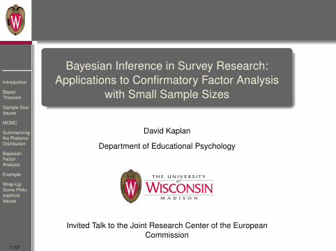
Bayesian Inference in Survey Research:Applications to Confirmatory Factor Analysis

with Small Sample Sizes

David Kaplan

Department of Educational Psychology

Invited Talk to the Joint Research Center of the EuropeanCommission

1 / 57

Introduction

Bayes’Theorem

Sample SizeIssues

MCMC



Example


This talk is drawn from my book Bayesian Statistics for theSocial Sciences, The Guilford Press, 2014.

2 / 57

Introduction

Bayes’Theorem

Sample SizeIssues

MCMC



Example


Introduction

Bayesian statistics has long been overlooked in the quantitativemethods training of social scientists.

Typically, the only introduction that a student might have toBayesian ideas is a brief overview of Bayes’ theorem whilestudying probability in an introductory statistics class.

1 Until recently, it was not feasible to conduct statistical modelingfrom a Bayesian perspective owing to its complexity and lack ofavailability.

2 Bayesian statistics represents a powerful alternative to frequentist(classical) statistics, and is therefore, controversial.

Recently, there has been a renaissance in the development andapplication of Bayesian statistical methods, owing mostly todevelopments of powerful statistical software tools that renderthe specification and estimation of complex models feasiblefrom a Bayesian perspective.

3 / 57

Introduction

Bayes’Theorem

Sample SizeIssues

MCMC



Example


Paradigm Differences

For frequentists, the basic idea is that probability is representedas long run frequency.

Frequentist probability underlies the Fisher andNeyman-Pearson schools of statistics – the conventionalmethods of statistics we most often use.

The frequentist formulation rests on the idea of equally probableand stochastically independent events

The physical representation is the coin toss, which relates tothe idea of a very large (actually infinite) number of repeatedexperiments.

4 / 57

Introduction

Bayes’Theorem

Sample SizeIssues

MCMC



Example


The entire structure of Neyman - Pearson hypothesis testingand Fisherian statistics (together referred to as the frequentistschool) is based on frequentist probability.

Our conclusions regarding the null and alternative hypothesespresuppose the idea that we could conduct the sameexperiment an infinite number of times.

Our interpretation of confidence intervals also assumes a fixedparameter and CIs that vary over an infinitely large number ofidentical experiments.

5 / 57

Introduction

Bayes’Theorem

Sample SizeIssues

MCMC



Example


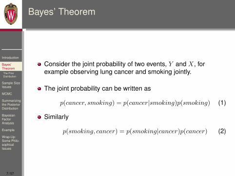
But there is another view of probability as subjective belief.

The physical model in this case is that of the “bet”.

Consider the situation of betting on who will win the the WorldCup (or the World Series).

Here, probability is not based on an infinite number ofrepeatable and stochastically independent events, but rather onhow much knowledge you have and how much you are willingto bet.

Subjective probability allows one to address questions such as“what is the probability that my team will win the World Cup?”Relative frequency supplies information, but it is not the sameas probability and can be quite different.

This notion of subjective probability underlies Bayesianstatistics.

6 / 57

Introduction

Bayes’TheoremThe PriorDistribution

Sample SizeIssues

MCMC



Example


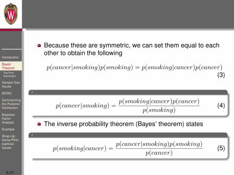
Bayes’ Theorem

Consider the joint probability of two events, Y and X, forexample observing lung cancer and smoking jointly.

The joint probability can be written as

p(cancer, smoking) = p(cancer|smoking)p(smoking) (1)

Similarly

p(smoking, cancer) = p(smoking|cancer)p(cancer) (2)

7 / 57

Introduction


Sample SizeIssues

MCMC



Example


Because these are symmetric, we can set them equal to eachother to obtain the following

p(cancer|smoking)p(smoking) = p(smoking|cancer)p(cancer)(3)

.

p(cancer|smoking) =p(smoking|cancer)p(cancer)

p(smoking)(4)

The inverse probability theorem (Bayes’ theorem) states.

p(smoking|cancer) =p(cancer|smoking)p(smoking)

p(cancer)(5)

8 / 57

Introduction


Sample SizeIssues

MCMC



Example


Why do we care?

Because this is how you could go from the probability of havingcancer given that the patient smokes, to the probability that thepatient smokes given that he/she has cancer.

We simply need the marginal probability of smoking and themarginal probability of cancer (”base rates” or what we will callprior probabilities).

9 / 57

Introduction


Sample SizeIssues

MCMC



Example


Statistical Elements of Bayes’ Theorem

What is the role of Bayes’ theorem for statistical inference?

Denote by Y a random variable that takes on a realized value y.For example, a person’s socio-economic status could beconsidered a random variable taking on a very large set ofpossible values.

This is the random variable Y . Once the person identifieshis/her socioeconomic status, the random variable Y is nowrealized as y.

Because Y is unobserved and random, we need to specify aprobability model to explain how we obtained the actual datavalues y.

10 / 57

Introduction


Sample SizeIssues

MCMC



Example


Next, denote by θ a parameter that we believe characterizes theprobability model of interest.

The parameter θ can be a scalar, such as the mean or thevariance of a distribution, or it can be vector-valued, such as aset of regression coefficients in regression analysis or factorloadings in factor analysis.

We are concerned with determining the probability of observingy given the unknown parameters θ, which we write as p(y|θ).

In statistical inference, the goal is to obtain estimates of theunknown parameters given the data.

This is expressed as the likelihood of the parameters given thedata, often denoted as L(θ|y).

11 / 57

Introduction


Sample SizeIssues

MCMC



Example


The key difference between Bayesian statistical inference andfrequentist statistical inference concerns the nature of theunknown parameters θ.

In the frequentist tradition, the assumption is that θ is unknown,but no attempt is made to account for our uncertainty about θ.

In Bayesian statistical inference, θ is also unknown but wereflect our uncertainty about the true value of θ by specifying aprobability distribution to describe it.

Because both the observed data y and the parameters θ areassumed random, we can model the joint probability of theparameters and the data as a function of the conditionaldistribution of the data given the parameters, and the priordistribution of the parameters.

12 / 57

Introduction


Sample SizeIssues

MCMC



Example


More formally,p(θ, y) = p(y|θ)p(θ). (6)

where p(θ, y) is the joint distribution of the parameters and thedata. Following Bayes’ theorem described earlier, we obtain

Bayes’ Theorem

p(θ|y) =p(θ, y)

p(y)=p(y|θ)p(θ)p(y)

, (7)

where p(θ|y) is referred to as the posterior distribution of theparameters θ given the observed data y.

13 / 57

Introduction


Sample SizeIssues

MCMC



Example


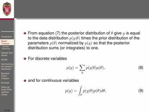
From equation (7) the posterior distribution of θ give y is equalto the data distribution p(y|θ) times the prior distribution of theparameters p(θ) normalized by p(y) so that the posteriordistribution sums (or integrates) to one.

For discrete variables

p(y) =∑θ

p(y|θ)p(θ), (8)

and for continuous variables

p(y) =

∫θ

p(y|θ)p(θ)dθ, (9)

14 / 57

Introduction


Sample SizeIssues

MCMC



Example


Notice that p(y) does not involve model parameters, so we canomit the term and obtain the unnormalized posterior distribution

.

p(θ|y) ∝ p(y|θ)p(θ). (10)

When expressed in terms of the unknown parameters θ for fixedvalues of y, the term p(y|θ) is the likelihood L(θ|y), which wedefined earlier. Thus, equation (10) can be re-written as

.

p(θ|y) ∝ L(θ|y)p(θ). (11)

15 / 57

Introduction


Sample SizeIssues

MCMC



Example


Equations (10) and (11) represents the core of Bayesianstatistical inference and is what separates Bayesian statisticsfrom frequentist statistics.

Equation (11) states that our uncertainty regarding theparameters of our model, as expressed by the prior densityp(θ), is weighted by the actual data p(y|θ) (or equivalently,L(θ|y)), yielding an updated estimate of our uncertainty, asexpressed in the posterior density p(θ|y).

16 / 57

Introduction


Sample SizeIssues

MCMC



Example


The Prior Distribution

Why do we specify a prior distribution on the parameters?

The key philosophical reason concerns our view that progressin science generally comes about by learning from previousresearch findings and incorporating information from thesefindings into our present studies.

The information gleaned from previous research is almostalways incorporated into our choice of designs, variables to bemeasured, or conceptual diagrams to be drawn.

Bayesian statistical inference simply requires that our priorbeliefs be made explicit, but then moderates our prior beliefs bythe actual data in hand.

Moderation of our prior beliefs by the data in hand is the keymeaning behind equations (10) and (11).

17 / 57

Introduction


Sample SizeIssues

MCMC



Example


But how do we choose a prior?

The choice of a prior is based on how much information webelieve we have prior to the data collection and how accurate webelieve that information to be.

This issue has also been discussed by Leamer (1983), whoorders priors on the basis of degree of confidence. Leamer’shierarchy of confidence is as follow: truths (e.g. axioms) > facts(data) > opinions (e.g. expert judgement) > conventions (e.g.pre-set alpha levels).

The strength of Bayesian inference lies precisely in its ability toincorporate existing knowledge into statistical specifications.

18 / 57

Introduction


Sample SizeIssues

MCMC



Example


Non-informative priors

In some cases we may not be in possession of enough priorinformation to aid in drawing posterior inferences.

From a Bayesian perspective, this lack of information is stillimportant to consider and incorporate into our statisticalspecifications.

In other words, it is equally important to quantify our ignoranceas it is to quantify our cumulative understanding of a problem athand.

The standard approach to quantifying our ignorance is toincorporate a non-informative prior into our specification.

Non-informative priors are also referred to as vague or diffusepriors.

19 / 57

Introduction


Sample SizeIssues

MCMC



Example


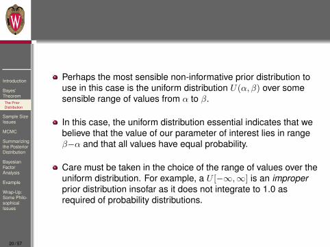
Perhaps the most sensible non-informative prior distribution touse in this case is the uniform distribution U(α, β) over somesensible range of values from α to β.

In this case, the uniform distribution essential indicates that webelieve that the value of our parameter of interest lies in rangeβ−α and that all values have equal probability.

Care must be taken in the choice of the range of values over theuniform distribution. For example, a U [−∞,∞] is an improperprior distribution insofar as it does not integrate to 1.0 asrequired of probability distributions.

20 / 57

Introduction


Sample SizeIssues

MCMC



Example


Informative-Conjugate Priors

It may be the case that some information can be brought tobear on a problem and be systematically incorporated into theprior distribution.

Such “subjective” priors are called informative.

One type of informative prior is based on the notion of aconjugate distribution.

A conjugate prior distribution is one that, when combined withthe likelihood function yields a posterior that is in the samedistributional family as the prior distribution.

21 / 57

Introduction


Sample SizeIssues

MCMC



Example


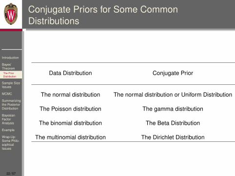
Conjugate Priors for Some CommonDistributions

Data Distribution Conjugate Prior

The normal distribution The normal distribution or Uniform Distribution

The Poisson distribution The gamma distribution

The binomial distribution The Beta Distribution

The multinomial distribution The Dirichlet Distribution

22 / 57

Introduction


Sample SizeIssues

MCMC



Example


−4 −2 0 2 4

0.0

0.5

1.0

1.5

Prior is Normal (0,0.3)

x

Density

prior

Likelihood

Posterior

−4 −2 0 2 4

0.0

0.5

1.0

1.5


x

Density

prior

Likelihood

Posterior

−4 −2 0 2 4

0.0

0.5

1.0

1.5


Density

prior

Likelihood

Posterior

−4 −2 0 2 4

0.0

0.5

1.0

1.5

Prior is Normal (0,3)

Density

prior

Likelihood

Posterior

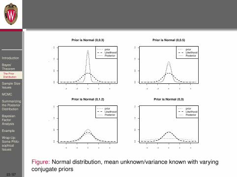
Figure: Normal distribution, mean unknown/variance known with varyingconjugate priors

23 / 57

Introduction


Sample SizeIssues

MCMC



Example


0 2 4 6 8 10

0.0

0.2

0.4

0.6

0.8

1.0

Prior is Gamma(10,0.2)

x

Den

sity

priorLikelihoodPosterior

0 2 4 6 8 10

0.0

0.2

0.4

0.6

0.8

1.0

Prior is Gamma(8,0.5)

x

Den

sity


0 2 4 6 8 10

0.0

0.2

0.4

0.6

0.8

1.0

Prior is Gamma(3,1)

Den

sity


0 2 4 6 8 10

0.0

0.2

0.4

0.6

0.8

1.0

Prior is Gamma(2.1,3)

Den

sity


Figure: Poisson distribution with varying gamma-density priors

24 / 57

Introduction

Bayes’Theorem

Sample SizeIssuesBayesian CLTand BayesShrinkage

MCMC



Example


Sample Size in Bayesian Statistics

In classical statistics, a re-occurring concern is the problem ofwhether a sample size is large enough to trust estimates andstandard errors.

This problem stems from the fact that the desirable propertiesof estimators such as OLS and ML exhibit themselves in thelimit as N approaches infinity.

The question is whether a finite sample size is large enough forthese desirable properties to “kick in”.

Considerable methodological work focuses on examining theeffects of small sample sizes on estimators in the context ofdifferent modeling frameworks.

25 / 57

Introduction

Bayes’Theorem


MCMC



Example


What is the role of sample size in Bayesian methods?

Because appeals to asymptotic properties are not part of theBayesian toolbox, can Bayesian statistics be used for smallsample sizes?

The answer depends on the interaction of the sample size withthe specification of the prior distribution.

This, in turn, can be seen from a discussion of the BayesianCentral Limit Theorem.

26 / 57

Introduction

Bayes’Theorem


MCMC



Example


Bayesian Central Limit Theorem andBayesian Shrinkage

As an example, assume that y follows a normal distributionwritten as

.

p(y|µ, σ2) =1√2πσ

exp

(− (y − µ)2

2σ2

). (12)

Specify a normal prior with mean and variancehyperparameters, κ and τ2, respectively which for this exampleare known.

.

p(µ|κ, τ2) =1√

2πτ2exp

(− (µ− κ)2

2τ2

). (13)

27 / 57

Introduction

Bayes’Theorem


MCMC



Example


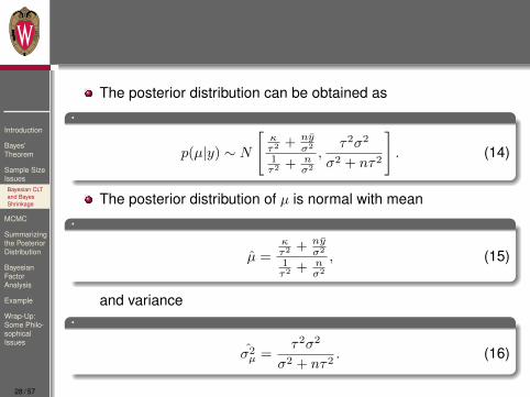
The posterior distribution can be obtained as.

p(µ|y) ∼ N

[κτ2 + ny

σ2

1τ2 + n

σ2

,τ2σ2

σ2 + nτ2

]. (14)

The posterior distribution of µ is normal with mean.

µ =κτ2 + ny

σ2

1τ2 + n

σ2

, (15)

and variance.

σ2µ =

τ2σ2

σ2 + nτ2. (16)

28 / 57

Introduction

Bayes’Theorem


MCMC



Example


Notice that as the sample size approaches infinity,.

limn→∞

µ = limn→∞

κτ2 + ny

σ2

1τ2 + n

σ2

,

= limn→∞

κσ2

nτ2 + yσ2

nτ2 + 1= y. (17)

Thus as the sample size increases to infinity, the expected aposteriori estimate µ converges to the maximum likelihoodestimate y.

With N very large is little information in the prior distribution thatis relevant to estimating the mean and variance of the posteriordistribution.

29 / 57

Introduction

Bayes’Theorem


MCMC



Example


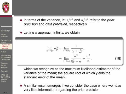
In terms of the variance, let 1/τ2 and n/σ2 refer to the priorprecision and data precision, respectively.

Letting n approach infinity, we obtain.

limn→∞

σ2µ = lim

n→∞

11τ2 + n

σ2

,

= limn→∞

σ2

σ2

τ2 + n=σ2

n, (18)

which we recognize as the maximum likelihood estimator of thevariance of the mean; the square root of which yields thestandard error of the mean.

A similar result emerges if we consider the case where we havevery little information regarding the prior precision.

30 / 57

Introduction

Bayes’Theorem


MCMC



Example


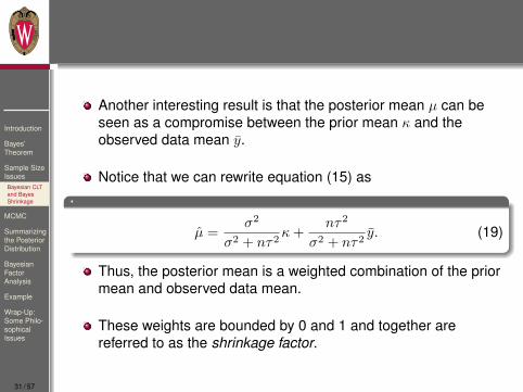
Another interesting result is that the posterior mean µ can beseen as a compromise between the prior mean κ and theobserved data mean y.

Notice that we can rewrite equation (15) as.

µ =σ2

σ2 + nτ2κ+

nτ2

σ2 + nτ2y. (19)

Thus, the posterior mean is a weighted combination of the priormean and observed data mean.

These weights are bounded by 0 and 1 and together arereferred to as the shrinkage factor.

31 / 57

Introduction

Bayes’Theorem


MCMC



Example


The shrinkage factor represents the proportional distance thatthe posterior mean has shrunk back to the prior mean κ andaway from the maximum likelihood estimator y.

If the sample size is large, the weight associated with κ willapproach zero and the weight associated with y will approachone. Thus µ will approach y.

Similarly, if the data variance σ2 is very large relative to the priorvariance τ2, this suggests little precision in the data relative tothe prior and therefore the posterior mean will approach theprior mean, κ.

Conversely, if the prior variance is very large relative to the datavariance this suggests greater precision in the data comparedto the prior and therefore the posterior mean will approach y.

32 / 57

Introduction

Bayes’Theorem


MCMC



Example


So, can Bayesian methods be used for very small samplesizes?

Yes, but the role of priors becomes crucial.

If sample size is small, the precision of the priors and theprecision of the data matter.

If the prior mean is way off with high precision, that is a problem.

Elicitation and model comparison is very important.

There is no free lunch!

33 / 57

Introduction

Bayes’Theorem

Sample SizeIssues

MCMC



Example


Markov Chain Monte Carlo Sampling

The key reason for the increased popularity of Bayesianmethods in the social and behavioral sciences has been the(re)-discovery of numerical algorithms for estimating theposterior distribution of the model parameters given the data.

Prior to these developments, it was virtually impossible toanalytically derive summary measures of the posteriordistribution, particularly for complex models with manyparameters.

Rather than attempting the impossible task of analyticallysolving for estimates of a complex posterior distribution, we caninstead draw samples from p(θ|y) and summarize thedistribution formed by those samples. This is referred to asMonte Carlo integration.

The two most popular methods of MCMC are the Gibbssampler and the Metropolis-Hastings algorithm.

34 / 57

Introduction

Bayes’Theorem

Sample SizeIssues

MCMC



Example


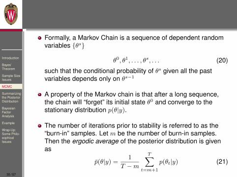
Formally, a Markov Chain is a sequence of dependent randomvariables θs

θ0, θ1, . . . , θs, . . . (20)

such that the conditional probability of θs given all the pastvariables depends only on θs−1

A property of the Markov chain is that after a long sequence,the chain will “forget” its initial state θ0 and converge to thestationary distribution p(θ|y).

The number of iterations prior to stability is referred to as the“burn-in” samples. Let m be the number of burn-in samples.Then the ergodic average of the posterior distribution is givenas

p(θ|y) =1

T −m

T∑t=m+1

p(θt|y) (21)

35 / 57

Introduction

Bayes’Theorem

Sample SizeIssues

MCMC

Summarizingthe PosteriorDistributionPointSummaries

IntervalSummaries


Example


Point Summaries of the Posterior Distribution

Hypothesis testing begins first by obtaining summaries ofrelevant distributions.

The difference between Bayesian and frequentist statistics isthat with Bayesian statistics we wish to obtain summaries of theposterior distribution.

The expressions for the mean and variance of the posteriordistribution come from expressions for the mean and varianceof conditional distributions generally.

Another common summary measure would be the mode of theposterior distribution – referred to as the maximum a posteriori(MAP) estimate.

36 / 57

Introduction

Bayes’Theorem

Sample SizeIssues

MCMC


IntervalSummaries


Example


Posterior Probability Intervals

In addition to point summary measures, it may also be desirableto provide interval summaries of the posterior distribution.

Recall that the frequentist confidence interval requires tweimagine an infinite number of repeated samples from thepopulation characterized by µ.

For any given sample, we can obtain the sample mean x and thenform a 100(1 − α)% confidence interval.

The correct frequentist interpretation is that 100(1 − α)% of theconfidence intervals formed this way capture the true parameter µunder the null hypothesis. Notice that the probability that theparameter is in the interval is either zero or one.

37 / 57

Introduction

Bayes’Theorem

Sample SizeIssues

MCMC


IntervalSummaries


Example


Posterior Probability Intervals (cont’d)

In contrast, the Bayesian framework assumes that a parameterhas a probability distribution.

Sampling from the posterior distribution of the model parameters,we can obtain its quantiles. From the quantiles, we can directlyobtain the probability that a parameter lies within a particularinterval.

So, a 95% posterior probability interval would mean that theprobability that the parameter lies in the interval is 0.95.

Notice that this is entirely different from the frequentistinterpretation, and arguably aligns with common sense.

38 / 57

Introduction

Bayes’Theorem

Sample SizeIssues

MCMC



Example


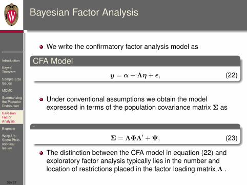
Bayesian Factor Analysis

We write the confirmatory factor analysis model as

CFA Model

y = α+ Λη + ε, (22)

Under conventional assumptions we obtain the modelexpressed in terms of the population covariance matrix Σ as

.

Σ = ΛΦΛ′ + Ψ, (23)

The distinction between the CFA model in equation (22) andexploratory factor analysis typically lies in the number andlocation of restrictions placed in the factor loading matrix Λ .

39 / 57

Introduction

Bayes’Theorem

Sample SizeIssues

MCMC



Example


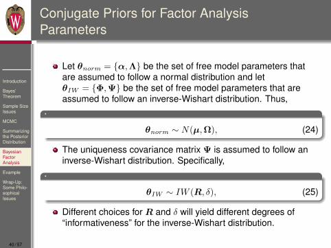
Conjugate Priors for Factor AnalysisParameters

Let θnorm = α,Λ be the set of free model parameters thatare assumed to follow a normal distribution and letθIW = Φ,Ψ be the set of free model parameters that areassumed to follow an inverse-Wishart distribution. Thus,

.

θnorm ∼ N(µ,Ω), (24)

The uniqueness covariance matrix Ψ is assumed to follow aninverse-Wishart distribution. Specifically,

.

θIW ∼ IW (R, δ), (25)

Different choices for R and δ will yield different degrees of“informativeness” for the inverse-Wishart distribution.

40 / 57

Introduction

Bayes’Theorem

Sample SizeIssues

MCMC



Example


Example

We present a small example of Bayesian factor analysis toillustrate the issue of sample size and precise priors.

Data come from a sample of 3500 10th grade students whoparticipated in the National Educational Longitudinal Study of1988.

Students were asked to respond to a series of questions thattap into their perceptions of the climate of the school.

A random sample of 100 respondents were obtained todemonstrate Bayesian CFA for sample sample sizes.

Smaller sample sizes are possible, but in this case, severeconvergence problems were encountered.

41 / 57

Introduction

Bayes’Theorem

Sample SizeIssues

MCMC



Example


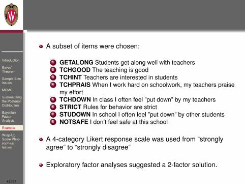
A subset of items were chosen:

1 GETALONG Students get along well with teachers2 TCHGOOD The teaching is good3 TCHINT Teachers are interested in students4 TCHPRAIS When I work hard on schoolwork, my teachers praise

my effort5 TCHDOWN In class I often feel ”put down” by my teachers6 STRICT Rules for behavior are strict7 STUDOWN In school I often feel ”put down” by other students8 NOTSAFE I don’t feel safe at this school

A 4-category Likert response scale was used from “stronglyagree” to “strongly disagree”

Exploratory factor analyses suggested a 2-factor solution.

42 / 57

Introduction

Bayes’Theorem

Sample SizeIssues

MCMC



Example


We use “MCMCfactanal” from the “MCMCpack” program withinthe R programming environment.

We specify 5000 burn-in iterations and 20,000 post-burn-initerations and a thinning interval of 20.

Summary statistics are based on 15,000 draws from theposterior distribution.

Using a thinning interval of 20, the trace and ACF plots indicateconvergence for the model parameters for the large sample sizecase.

Some convergence problems were noted for the small samplesize case.

43 / 57

Introduction

Bayes’Theorem

Sample SizeIssues

MCMC



Example


Table: Results of Bayesian CFA: N=3500 and Noninformative Priors.

Parameter EAP SD 95% PPI

N=3500 / Noninformative Prior

Loadings: POSCLIM byTCHGOOD 0.81 0.02 0.76, 0.85TCHERINT 0.89 0.02 0.85, 0.93TCHPRAIS 0.59 0.02 0.55, 0.63

Loadings: NEGCLIM bySTRICT 0.09 0.01 0.06, 0.13SPUTDOWN 0.32 0.01 0.28, 0.35NOTSAFE 0.30 0.02 0.26, 0.35

44 / 57

Introduction

Bayes’Theorem

Sample SizeIssues

MCMC



Example


Table: Results of Bayesian CFA: N=100 and Noninformative Priors.


N=100 / Noninformative Prior



45 / 57

Introduction

Bayes’Theorem

Sample SizeIssues

MCMC



Example


Table: Results of Bayesian CFA: N=3500 and Informative Priors.


N=3500 / Informative Prior



46 / 57

Introduction

Bayes’Theorem

Sample SizeIssues

MCMC



Example


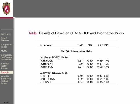
Table: Results of Bayesian CFA: N=100 and Informative Priors.


N=100 / Informative Prior



47 / 57

Introduction

Bayes’Theorem

Sample SizeIssues

MCMC



Example


Wrap-Up: Some Philosophical Issues

Bayesian statistics represents a powerful alternative tofrequentist (classical) statistics, and is therefore, controversial.

The controversy lies in differing perspectives regarding thenature of probability, and the implications for statistical practicethat arise from those perspectives.

The frequentist framework views probability as synonymouswith long-run frequency, and that the infinitely repeatingcoin-toss represents the canonical example of the frequentistview.

In contrast, the Bayesian viewpoint regarding probability was,perhaps, most succinctly expressed by de Finetti

48 / 57

Introduction

Bayes’Theorem

Sample SizeIssues

MCMC



Example


.Probability does not exist.

- Bruno de Finetti

49 / 57

Introduction

Bayes’Theorem

Sample SizeIssues

MCMC



Example


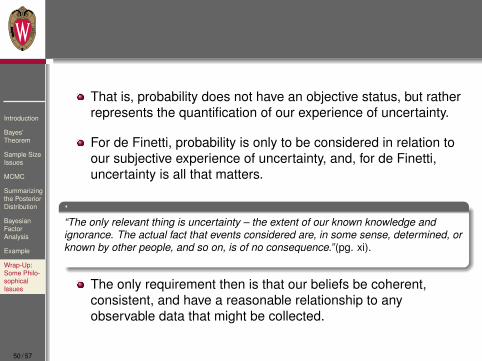
That is, probability does not have an objective status, but ratherrepresents the quantification of our experience of uncertainty.

For de Finetti, probability is only to be considered in relation toour subjective experience of uncertainty, and, for de Finetti,uncertainty is all that matters.

.“The only relevant thing is uncertainty – the extent of our known knowledge andignorance. The actual fact that events considered are, in some sense, determined, orknown by other people, and so on, is of no consequence.” (pg. xi).

The only requirement then is that our beliefs be coherent,consistent, and have a reasonable relationship to anyobservable data that might be collected.

50 / 57

Introduction

Bayes’Theorem

Sample SizeIssues

MCMC



Example


Subjective v. Objective Bayes

There are controversies within the Bayesian school between“subjectivists and “objectivists

Subjective Bayesian practice attempts to bring prior knowledgedirectly into an analysis. This prior knowledge represents theanalysts (or others) degree-of-uncertainity.

An analyst’s degree-of-uncertainty is encoded directly into thespecification of the prior distribution, and in particular on thedegree of precision around the parameter of interest.

The advantages include

1 Priors can be based on factual prior knowledge

2 Small sample sizes can be handled.

51 / 57

Introduction

Bayes’Theorem

Sample SizeIssues

MCMC



Example


For objectivists, the goal is to have the data speak as much aspossible, but to allow priors that serve as objective “referents“.

Specifically, there are a large class of so-called reference priors(Kass and Wasserman,1996).

An important viewpoint regarding the notion of objectivity in theBayesian context comes from Jaynes (1968).

For Jaynes, the “personalistic” (subjective) school of probabilityis to be reserved for

.“...the field of psychology and has no place in applied statistics. Or, tostate this more constructively, objectivity requires that a statistical analysisshould make use, not of anybody’s personal opinions, but rather thespecific factual data on which those opinions are based.”(pg. 228)

52 / 57

Introduction

Bayes’Theorem

Sample SizeIssues

MCMC



Example


Evidenced-based Subjective Bayes

The subjectivist school, advocated by de Finetti and others,allows for personal opinion to be elicited and incorporated into aBayesian analysis. In the extreme, the subjectivist school wouldplace no restriction on the source, reliability, or validity of theelicited opinion.

The objectivist school advocated by Jeffreys, Jaynes, Berger,Bernardo, and others, views personal opinion as the realm ofpsychology with no place in a statistical analysis. In theirextreme form, the objectivist school would require formal rulesfor choosing reference priors.

The difficulty with these positions lies with the everyday usageof terms such as “subjective” and “belief”.

Without careful definitions of these terms, their everyday usagemight be misunderstood among those who might otherwiseconsider adopting the Bayesian perspective.

53 / 57

Introduction

Bayes’Theorem

Sample SizeIssues

MCMC



Example


“Subjectivism” within the Bayesian framework runs the gamutfrom the elicitation of personal beliefs to making use of the bestavailable historical data available to inform priors.

I argue along the lines of Jaynes (1968) – namely that therequirements of science demand reference to “specific, factualdata on which those opinions are based” (pg. 228).

This view is also consistent with Leamer’s hierarchy ofconfidence on which priors should be ordered.

We may refer to this view as an evidence-based form ofsubjective Bayes which acknowledges (1) the subjectivity thatlies in the choice of historical data; (2) the encoding of historicaldata into hyperparameters of the prior distribution; and (3) thechoice among competing models to be used to analyze thedata.

54 / 57

Introduction

Bayes’Theorem

Sample SizeIssues

MCMC



Example


What if factual historical data are not available?

Berger (2006) states that reference priors should be used “inscenarios in which a subjective analysis is not tenable”,although such scenarios are probably rare.

The goal, nevertheless, is to shift the practice of Bayesianstatistics away from the elicitation of personal opinion (expert orotherwise) which could, in principle, bias results toward aspecific outcome, and instead move Bayesian practice towardthe warranted use prior objective empirical data for thespecification of priors.

The specification of any prior should be explicitly warrantedagainst observable, empirical data and available for critique bythe relevant scholarly community.

55 / 57

Introduction

Bayes’Theorem

Sample SizeIssues

MCMC



Example


To conclude, the Bayesian school of statistical inference is,arguably, superior to the frequentist school as a means ofcreating and updating new knowledge in the social sciences.

An evidence-based focus that ties the specification of priors toobjective empirical data provides stronger warrants forconclusions drawn from a Bayesian analysis.

In addition, predictive criteria should always be used as ameans of testing and choosing among Bayesian models.

As always, the full benefit of the Bayesian approach to researchin the social sciences will be realized when it is more widelyadopted and yields reliable predictions that advance knowledge.

56 / 57

Introduction

Bayes’Theorem

Sample SizeIssues

MCMC



Example


.

GRAZIE MILLE

57 / 57

Bayesian Inference in Survey Research: Applications to ... · Introduction Bayes’ Theorem Sample...

Documents

Transcript of Bayesian Inference in Survey Research: Applications to ... · Introduction Bayes’ Theorem Sample...