Bayesian Hyperspectral Image Segmentation With ...bioucas/files/ieee_tgars_2011_fsmlr.pdf · IEEE...

IEEE TRANSACTIONS ON GEOSCIENCE AND REMOTE SENSING, VOL. 49, NO. 6, JUNE 2011 2151

Bayesian Hyperspectral Image SegmentationWith Discriminative Class Learning

Janete S. Borges, José M. Bioucas-Dias, Member, IEEE, and Andre R. S. Marcal

Abstract—This paper introduces a new supervised technique tosegment hyperspectral images: the Bayesian segmentation basedon discriminative classification and on multilevel logistic (MLL)spatial prior. The approach is Bayesian and exploits both spectraland spatial information. Given a spectral vector, the posteriorclass probability distribution is modeled using multinomial logisticregression (MLR) which, being a discriminative model, allowsto learn directly the boundaries between the decision regionsand, thus, to successfully deal with high-dimensionality data. Tocontrol the machine complexity and, thus, its generalization ca-pacity, the prior on the multinomial logistic vector is assumedto follow a componentwise independent Laplacian density. Thevector of weights is computed via the fast sparse multinomiallogistic regression (FSMLR), a variation of the sparse multinomiallogistic regression (SMLR), conceived to deal with large data setsbeyond the reach of the SMLR. To avoid the high computationalcomplexity involved in estimating the Laplacian regularizationparameter, we have also considered the Jeffreys prior, as it does notdepend on any hyperparameter. The prior probability distributionon the class-label image is an MLL Markov–Gibbs distribution,which promotes segmentation results with equal neighboring classlabels. The α-expansion optimization algorithm, a powerfulgraph-cut-based integer optimization tool, is used to computethe maximum a posteriori segmentation. The effectiveness of theproposed methodology is illustrated by comparing its performancewith the state-of-the-art methods on synthetic and real hyperspec-tral image data sets. The reported results give clear evidence ofthe relevance of using both spatial and spectral information inhyperspectral image segmentation.

Index Terms—Bayesian methods, hyperspectral imaging, imageclassification, image segmentation.

I. INTRODUCTION

HYPERSPECTRAL sensors acquire spectral informationin an almost continuous fashion, yielding a high discrim-

ination capacity between different land-cover classes. However,the high dimensionality of hyperspectral images raises diffi-culties frequently related with the Hughes phenomenon [1],

Manuscript received April 23, 2010; revised August 27, 2010 andOctober 14, 2010; accepted November 16, 2010. Date of publicationJanuary 19, 2011; date of current version May 20, 2011. This work wassupported by the Centro de Investigação em Ciências Geo-Espaciais underProject MRTN-CT-2006-035927 (Hyperspectral Imaging Network). The workof J. S. Borges was supported by the Fundação para a Ciência e a Tecnologiaunder Grant SFRH/BD/17191/2004.

J. S. Borges and A. R. S. Marcal are with the Centro de Investigaçãoem Ciências Geo-Espaciais, Departamento de Matemática Aplicada, Facul-dade de Ciências, Universidade do Porto, 4169-007 Porto, Portugal (e-mail:[email protected]; [email protected]).

J. M. Bioucas-Dias is with the Instituto de Telecomunicações and InstitutoSuperior Técnico, Universidade Técnica de Lisboa, 1049-001 Lisboa, Portugal(e-mail: [email protected]).

Digital Object Identifier 10.1109/TGRS.2010.2097268

which limits the range of applicable classification/segmentationalgorithms.

The supervised learning methods in high-dimensional spacesrequire a large number of training samples to correctly estimatethe parameters of the underlying model. This brings abouttwo problems. First, the access to a consistent set with asufficient number of training samples is often impossible orhighly costly. Second, the use of large training sets in high-dimensional spaces leads to expensive computational demands.Several segmentation and classification methods are currentlybeing developed to address these problems [2]–[7].

A. Discriminative Approaches to Hyperspectral Classification

Discriminative class learning algorithms are usually lesscomplex than their generative counterparts because they modeldirectly the posterior class densities [8]–[10]. A conceptuallysimpler approach to classification is to learn the so-calleddiscriminant functions which encode the boundary betweenclasses [10].

Discriminative approaches are among the state of the art inthe classification of high-dimensional data, such as hyperspec-tral vectors. The multinomial logistic regression (MLR) [11],which models the posterior class probability distributions, andthe support vector machines (SVMs) [12], which are discrimi-nant functions, have been successfully applied to the classifica-tion of high-dimensional data sets. SVMs are probably the mostpopular discriminative approach applied to the classificationof remotely sensed data [7], [13]–[18], where the ability ofSVMs in dealing with large input spaces and producing sparsesolutions has been largely demonstrated. In this paper, however,we use the MLR because this model yields the posterior classprobability distributions, which play a crucial role regarding theintroduction of spatial information. Although effective sparseMLR (SMLR) methods are available [19], [20], their use inremotely sensed data classification is not as popular as SVMs.

B. Exploiting Spatial Information

It is of common sense that neighboring pixels in remotelysensed images very likely have the same class label. Therefore,the classification of remotely sensed images, as well as anyother type of real-world images, is expected to improve whensome sort of spatial information is included in the inference ofthe class labels. In this paper, we adopt a multilevel logistic(MLL) Markov random field (MRF) [21] to model the piece-wise smooth nature of the images of class labels. The workpresented here is a consequence of the works developed andpresented in [22] and [23].

0196-2892/$26.00 © 2011 IEEE

2152 IEEE TRANSACTIONS ON GEOSCIENCE AND REMOTE SENSING, VOL. 49, NO. 6, JUNE 2011

Although MRFs have been widely used in the remote sensingcommunity [2], [24], [25], its interest has reemerged recentlyowing to the introduction of powerful integer optimization toolsbased on graph-cut techniques. The ability of MRFs to integratespatial context into image classification problems has beenexploited by several authors. The integration of SVM tech-niques within an MRF framework for accurate spectral–spatialclassification of remote sensing images was exploited by Farag[26], Bruzzone [27], and Gong [28] research groups. The useof an MRF framework to model the spatial neighborhood ofa pixel in hyperspectral images can be found in [6] and [24].Tarabalka et al. [24] present an SVM- and MRF-based methodthat comprises two steps: First, a probabilistic SVM pixelwiseclassification of the hyperspectral image is performed, followedby MRF-based regularization for incorporating spatial andedge information into the classification. Another example ofa Markov-based classification framework is presented in [6]where a neurofuzzy classifier is used to perform classificationin the spectral domain and compute a first approximation ofthe posterior probabilities, and the resulting output is then fedto an MRF spatial analysis stage combined with a maximumlikelihood (ML) probabilistic reclassification.

In addition to MRF-based approaches, extended morpholog-ical profiles were also considered to integrate spatial informa-tion in the classification of hyperspectral images [6], as wellas a composite kernel methodology [29]. Another approachconsidered consists in performing segmentation and pixelwiseclassification independently and then combining the resultsusing a majority voting rule, for example, in [30], where awatershed technique has been used to perform segmentationand an SVM pixelwise classification is performed, followed bymajority voting in the watershed regions.

More recently, graph-based methods have also been pro-posed for spectral–spatial classification of hyperspectral im-ages [31] by constructing a minimum spanning forest rootedon the markers selected by using pixelwise classificationresults.

C. Proposed Approach

In this paper, we present a Bayesian segmentation procedurebased on the MLR discriminative classifier, which accounts forthe spectral information, and on the MLL prior, which accountsfor the spatial information. Accordingly, we term the methodBayesian segmentation based on discriminative classificationand on MLL spatial prior (BSD-MLL). The BSD-MLL methodcomprises two parts: 1) the estimation of the MLR regressorsand 2) the segmentation of the images by computing themaximum a posteriori (MAP) labeling based on the posteriorMLR and on the MLL spatial prior. The parameters requiredfor each part of the process are learned in two consecutive, butnonsimultaneous, steps. Although this procedure is suboptimal,it is much lighter than the optimal one, and nevertheless, as wewill give evidence, it yields state-of-the-art results.

The MLR regressors are estimated using a new algorithm thatis inspired in the SMLR [19] but much faster and able to copewith data sets far beyond the reach of the SMLR. Accordingly,we name this algorithm fast SMLR (FSMLR).

To enforce sparsity and, in this way, control the classifiercomplexity, the SMLR uses a Laplacian prior for the regressors.

This prior depends on a parameter which plays the role ofthe regularization parameter. The inference of this parameteris usually complex from the computational point of view. Tosidestep this difficulty, the noninformative Jeffreys prior [32]is also considered in this paper because, while still leading tosparse solutions, it does not depend on any parameter yielding,therefore, lighter estimation procedures.

In computing the MAP segmentation, one faces a hard inte-ger optimization problem, which we solve by using the pow-erful graph-cut-based α-expansion algorithm [33]. It yields anexact solution in the binary case and a very good approximationwhen there are more than two classes.

The performance of the proposed BSD-MLL algorithm isillustrated in a set of experiments carried out in differentconditions with synthetic and simulated data, regarding the sizeof the training set. Both the step for the estimation of MLRregressors and the segmentation step are evaluated separately,and the results are compared with state-of-the-art hyperspectralclassification/segmentation methods.

In addition to the fact that the BSD-MLL algorithm is com-petitive with state-of-the-art classification methods for hyper-spectral images, it is important to emphasize that the proposedalgorithm reveals other important advantages: 1) It models ac-curately the piecewise continuous nature of the image elementsby means of the MLL spatial prior, and 2) it is efficient (fromthe computational point of view) and provides high-qualityapproximate solutions to the hard integer optimization problemthrough the use of the α-expansion algorithm.

This paper is organized in four sections, with Section I beingthe Introduction. Section II presents the problem formulationwhere we start by reviewing the core concepts of the SMLRin Section II-A with both the Laplacian (see Section II-A1)and Jeffreys priors (see Section II-A2), and then, the FSMLRis proposed in Section II-A3. Section II carries on with theinclusion of contextual information in the classification process,achieved through the introduction of an MLL Markov–Gibbsprior (see Section II-B). The problem formulation section isconcluded with the MAP segmentation description with theα-expansion algorithm (see Section II-C). Section III presentsthe results of the application of the proposed algorithms(FSMLR for classification and BSD-MLL for segmentation)(considering different conditions based on the type of prior,the type of input function, and the inclusion of contextualinformation) to simulated data sets (see Section III-A) andIndian Pines (see Section III-B) and Pavia (see Section III-C)benchmarked data sets. The final discussions and conclusionsare presented in Section IV.

II. PROBLEM FORMULATION

Let x = {xi ∈ Rd, i ∈ S} denote an observed hyperspectralimage, also termed the image of features, where d is the numberof spectral bands and S is the set of pixels in the scene. The goalof classification is to assign a label yi ∈ L = {1, 2, . . . ,K} toeach i ∈ S , based on the vector xi, resulting in an image ofclass labels y = {yi|i ∈ S}. We call this assignment a labeling.The goal of segmentation is, based on the observed image x, tocompute a partition S = ∪iSi of the set S such that the pixels ineach element of the partition share some common property, forexample, to belong to the same land-cover type. Notice that,

BORGES et al.: BAYESIAN HYPERSPECTRAL IMAGE SEGMENTATION 2153

given a labeling y, the collection Sk = {i ∈ S|yi = k}, fork = 1, . . . ,K, is a partition of S . On the other hand, given thesegmentation Sk, for k = 1, . . . ,K, the image {yi|yi = k if i ∈Sk, i ∈ S} is a labeling. There is, therefore, a one-to-one rela-tion between labelings and segmentations. Nevertheless, in thispaper, we use the term classification when there is no spatialinformation and segmentation when the spatial prior is beingconsidered.

In a Bayesian framework, the estimation of y having ob-served x is done by maximizing the posterior distribution1

p(y|x) ∝ p(x|y)p(y) (1)

where p(x|y) is the likelihood function (i.e., the probability ofthe feature image x given the labeling y) and p(y) is the priorover the class labels.

Discriminative classifiers learn directly p(y|x), the posteriorclass-label probability distribution, given the features. In thispaper, we develop a fast version of the SMLR classifier [34],which we name FSMLR, to learn the posterior class probabilitydistribution p(yi|xi). The FSMLR is suited to problems withmany classes and is able to cope with problems far beyond thereach of the SMLR.

The likelihood function is given by p(xi|yi) =p(yi|xi)p(xi)/p(yi). Since p(xi) does not depend on thelabeling y, we have

p(x|y) ∝∏i∈S

p(yi|xi)/p(yi) (2)

where conditional independence is understood.In this approach, the classes are assumed as likely probable:

p(yi) = 1/K. Although this assumption may not be the ideal,it still leads to very good results. The class probability distri-butions may be tilted, if required, toward other distributions byusing the method described in [35].

A. Estimation of the Class Probability DistributionsUsing SMLR

In this section, we briefly review the core concepts of theSMLR. We follow closely [19]. The SMLR algorithm learnsa multiclass classifier based on the MLR. By incorporating aprior, this method simultaneously performs feature selection toidentify a small subset of the most relevant features and learnsthe classifier itself.

Let x ≡ [x1, . . . , xd]T ∈ Rd be d observed features. The

goal of the MLR is to assign to each xi, for i ∈ S , theprobability of belonging to each of the K classes. Let y ≡[y(1), . . . , y(K)]

Tdenote a 1-of-K encoding vector of the K

classes, such that y(k) = 1 if xi corresponds to an exam-ple belonging to class k and y(k) = 0 otherwise, and w ≡[w(1)T , . . . ,w(K)T ]

Tdenotes the so-called regression of the

feature weight vector composed of K feature regression vectors

1To keep the notation light, we denote both probability densities and proba-bility distributions with p(·). Furthermore, the random variable to which p(·)refers is to be understood from the context.

w(k), for k = 1, . . . ,K. With these definitions in place, theprobability that a given sample xi belongs to class k is given by

p(y(k) = 1|xi,w

)=

exp(w(k)Th(xi)

)∑K

k=1 exp(w(k)Th(xi)

) (3)

where h(xi) = [h1(xi), . . . , hl(xi)]T [(·)T denotes the

transpose operation] is a vector of l fixed functions of theinput, often termed features. Since p(y(k) = 1|xi,w) does notdepend on a translation on w, we set w(K) ≡ 0.

Possible choices for function h are linear (i.e., h(xi) =[1, xi,1, . . . , xi,d]

T , where xi,j is the jth component of xi)and kernel (i.e., h(x) = [1, K(x,x1), . . . , K(x,xm)]T , whereK(·, ·) is some symmetric kernel function). Kernels are nonlin-ear mappings, thus ensuring that the transformed samples aremore likely to be linearly separable. A popular kernel used inimage classification is the Gaussian radial basis function (RBF):K(x, z) = − exp(|x− z|2/(2σ2

h)).In a supervised learning context, the components of

w are estimated from the training data D ≡ {(xi1 ,yi1),. . . , (xim ,yim)}. Usually, this estimation is done using the MLprocedure to obtain the components of w from the training data,i.e., the ML estimate wML is obtained by maximizing the log-likelihood function [36]

l(w) =

m∑i=1

[K∑

k=1

y(k)i w(k)Txi − log

K∑k=1

exp(w(k)Txi

)].

(4)

A sparsity-promoting prior p(w) is incorporated in the infer-ence of vector w in order to achieve sparsity in the estimate ofw. The prior will control the classifier complexity and, there-fore, its generalization capacity. In addition, the introduction ofa prior on w will also prevent the unbounded growth of the log-likelihood function when the training data are separable.

With the inclusion of a prior on w, the MAP criterion is usedinstead of the popular ML one for the MLR. The estimate of wis then given by

wMAP = argmaxw

L(w) (5)

= argmaxw

[l(w) + log p(w)] . (6)

Several works on MLR [2], [19] have adopted the zero-meanLaplacian prior

p(w) ∝ exp (−λ‖w‖1)

where

‖w‖1 =

d(K−1)∑i=1

|wi|

denotes the �1 norm of w and λ is a hyperparameter playingthe role of the regularization parameter, controlling the degreeof sparseness of the estimates obtained. The inclusion of the�1 norm in (6) yields sparse regressors wMAP, i.e., regressorswith many components set to zero [19]. In this way, the com-plexity of the machine is controlled, ensuring its generalizationcapability. We note that the nonzero coefficients select features(bands) in the case of linear kernels or support vectors in thecases of nonlinear kernels.


The process of selecting the optimum λ is usually doneby cross validation through the training process. In high-dimensional data sets, such as hyperspectral images, this searchoften becomes a time-consuming task. In order to mitigate thiscomputational burden, we also consider the Jeffreys prior [32]

p(w) ∝d(K−1)∏

i=1

1

|wi|(7)

which, as the Laplacian prior, also enforces sparseness but doesnot depend on any parameter to tune, thus leading to a lighterlearning algorithm.

We start by briefly describing the SMLR algorithm proposedin [19], and then, we introduce our FSMLR approach to inferthe regression vector w, both for the Laplacian and Jeffreyspriors.

1) SMLR With Laplacian Prior: The �1 norm is nonsmooth,preventing the use of standard optimization tools based onderivatives. The bound optimization [37] framework suppliesadequate tools to address nonsmooth optimization. The centralconcept in bound optimization is the replacement of a difficultoptimization problem, in this case, L(w) = l(w) + log p(w),with a sequence of surrogate functions simpler to optimize [37].Let Q(w|w(t)) denote the surrogate function, where w(t) isthe regression vector computed at iteration t. This function isdesigned such that the difference

L(w)−Q(w|w(t)

)(8)

is minimized at w = w(t). Let

w(t+1) = argmaxw

Q(w|w(t)

). (9)

A straightforward calculus leads to the conclusion that

L(w(t+1)

)≥ L

(w(t)

)(10)

i.e., the sequence {L(w(t+1)), t = 0, 1, . . .} is nondecreasing.Under suitable conditions, this sequence converges to the max-imum of L [37].

As previously stated, function Q should be easy to optimize,and thus, quadratic functions come immediately to mind. Sincel(w) is concave and belongs to C2, a surrogate function for l,denoted as Ql(w|w′), can be determined using a bound on itsHessian H. Let

B ≡ −1

2[I− 11T /K]⊗

m∑i=1

xixTi (11)

where 1 ≡ [1, 1, . . . , 1]T and ⊗ denote the Kronecker product.Matrix B is nonpositive, and H(w)−B is positive semidefi-nite, i.e., H(w) B for any w [11]. A valid surrogate functionfor l is then

Q(w|w(t)

)≡

(w − w(t)

)Tg(w(t)

)+

1

2

(w − w(t)

)TB

(w − w(t)

)(12)

= wT(g(w(t)

)−Bw(t)

)+

1

2wTBw + c (13)

where c is an irrelevant constant and g is the gradient of lgiven by

g(w) =m∑i=1

(y′i − pi(w))⊗ xi (14)

with y′i≡ [y

(1)i , y

(2)i , . . . , y

(K−1)i ]

Tand pi(w)≡ [p

(1)i (w), . . . ,

p(K−1)i (w)]T , where p

(k)i (w) ≡ p(y

(k)i = 1|xi,w).

Concerning the �1 norm |w|1 =∑

i |wi|, we note that forwi,(t) �= 0

−|wi| ≥ −1

2

w2i∣∣wi,(t)

∣∣ + cte (15)

where cte is a constant. Thus, both terms of L(w) have aquadratic bound. Since the sum of functions is lower boundedby the sum of the correspondent lower bounds, we have aquadratic bound for L(w) given by

Q(w|w(t)

)= wT

(g(w(t)

)−Bw(t)

)+

1

2wTBw +

1

2wTΛ(t)w (16)

where

Λ(t) ≡ diag{∣∣w1,(t)

∣∣−1, . . . ,

∣∣wd(K−1),(t)

∣∣−1}. (17)

The maximization of (16) leads to

w(t+1) =(B− λΛ(t)

)−1 (Bw(t) − g

(w(t)

)). (18)

The terms |wi,(t)|−1, present in the diagonal of matrix Λ(t),tend to infinity when wi,(t) approaches to zero. We can thusforesee numerical problems in the successive computations of(18) because the �1 norm does enforce many elements of w tobe zero. These numerical difficulties are, however, sidesteppedby computing (18) using the following equivalent expression:

w(t+1) = Γ(t)

(Γ(t)BΓ(t) − λI

)−1Γ(t)

(Bw(t) − g(w(t))

)(19)

where

Γ(t) ≡ diag{∣∣w1,(t)

∣∣1/2 , . . . , ∣∣wd(K−1),(t)

∣∣1/2} . (20)

Notice that (19) is well defined since matrix Γ(t)BΓ(t) − λI isnegative definite.

The algorithm just presented is reminiscent of the iterativereweighted least squares (IRLS) used for the ML estimationof the vector w (see [38]). In fact, each IRLS iteration has thesame computational complexity of (19). We, thus, compute theexact MAP MLR under a Laplacian prior with the same cost asthe original IRLS algorithm for ML estimation.

An important issue remains: the adjustment of the sparsenessparameter λ in (19). As previously referred, this adjustmentshould be done by cross validation, which results in a time-consuming task. To avoid this, a Jeffreys prior on the weights isalso considered. We next describe how the MLR is performedwith this prior.


2) SMLR With Jeffreys Prior: The Jeffreys prior given in (7)leads the objective function

L(w) = l(w)−d(K−1)∑

i=1

log |wi|. (21)

In place of the term λ|wi| that we had in the Laplace prior, wehave now the term log |wi| for the Jeffreys prior. Given that,from small perturbations of wi about w′

i, we have log |wi| �|wi|/|w′

i|+ c, we conclude that the Jeffreys prior acts as theLaplacian one with an adaptive parameter λ = 1/|w′

i|, thusforcing aggressively the small elements of the regressor w tobe zero. The Jeffreys prior is in fact known as a strong sparsity-promoting prior [39]. This characteristic will be evident also inthe experiments reported in Section III.

To maximize L(w), we use, as before, the bound optimiza-tion framework. In this way, the surrogate function Q(w|w(t))for l(w) given by (13) is kept. Concerning the logarithm of theJeffreys prior, a straightforward calculus leads to the inequality

− log |wi| ≥ −1

2

w2i∣∣wi,(t)

∣∣2 + cte (22)

where cte denotes a constant depending only on wi,(t). Sincethe minimum of − log |wi| − (−1/2w2

i /|wi,(t)|2) is reachedat wi = wi,(t), then −1/2w2

i /|wi,(t)|2 is a valid surrogatefunction for − log |wi|, and by comparing (22) with (15), weconclude that w(t+1) is the same as that in (18), where thematrix Λ(t) is now given by

Λ(t) ≡ diag{∣∣w1,(t)

∣∣−2, . . . ,

∣∣wd(K−1),(t)

∣∣−2}. (23)

As with the Laplacian prior, we may write

w(t+1) = Γ(t)

(Γ(t)BΓ(t) − I

)−1Γ(t)

(Bw(t) − g

(w(t)

))(24)

where

Γ(t) ≡ diag{∣∣w1,(t)

∣∣ , . . . , ∣∣wd(K−1),(t)

∣∣} . (25)

The terms − log |wi| present in (21) are nonconcave, andtherefore, the correspondent objective function L(w) is not,with generality, concave. Therefore, we are not guaranteed toobtain the global maxima. However, as shown in Section III, byinitializing all elements of w with nonzero values, we obtainsystematically very good estimates of w.

3) FSMLR—BGS Iterations: Independent of the prior used,the computational cost of solving, at each iteration, the linearsystems implicit in (19) and (24) is on the order of ((dK)3),preventing the application of SMLR to data sets with largevalues of the product dK. This is the scenario that we havein most hyperspectral image classification, or segmentation,problems. Even using linear kernels and, thus, values of don the order of a few hundreds, the number of classes isfrequently on the order of 20, leading to matrices of thousandsby thousands, let alone the kernel case. In order to circumventthis problem, a modification to the iterative method used in theSMLR is introduced. This modification results in a faster andmore efficient algorithm: the FSMLR [34]. The FSMLR uses

the block Gauss–Seidel (BGS) method [38] to solve the systemimplicit in (24). The modification consists in, at each iteration,solving blocks corresponding to the weights belonging to thesame class, instead of computing the complete set of weights.

The linear system in (19) and (24) can be written as Au =z, where A ≡ (Γ(t)BΓ(t) − λI) and z ≡ Γ(t)(Bw(t) −g(w(t))) wherein w(t+1) = Γ(t)u and Γ(t) is given by (20)for the Laplacian prior and by (25) for the Jeffreys prior. Theregularization parameter takes the value λ = 1 in the case ofthe Jeffreys prior.

Computing w(t+1) is thus equivalent to solving the systemAu = z with respect to u and then computing w(t+1) =

Γ(t)w(t+1)u.Recall that Γ(t) is a diagonal matrix made of K − 1 diagonal

blocks of size d× d; the kth diagonal block corresponds to thekth class. Hence, Γ(t) has dimension (d(K − 1))× (d(K −1)). Matrix B (11) has dimension (d(K − 1))× (d(K − 1)),and it can be decomposed into d× d blocks Bik given by

Bik ≡[−1

2[I− 11T /K]

]ik

Rx, i, k = 1, . . . ,K − 1

(26)

where Rx ≡∑m

i=1 xixTi . With this definition in place and by

setting z and u as block vectors, where zk and uk are theblocks corresponding to the class k, we have concluded thatsolving the linear systems Au = z with the BGS iterativeprocedure is equivalent to solving⎡⎢⎣ A1,1 . . . A1,K−1

......

AK−1,1 . . . AK−1,K−1

⎤⎥⎦⎡⎣ u1

...uK−1

⎤⎦ =

⎡⎣ z1...

zK−1

⎤⎦ (27)

where

Aik = Γi,(t)BikΓk,(t) − λI (28)

and Γk,(t) is the kth block diagonal matrix of Γk correspondingto the class k.

Using this technique, it happens that, at each iteration, K sys-tems of equal dimension to the number of samples are solved.This results in an improvement in terms of computational efforton the order of K2, which has a high impact in problems witha large number of classes.

The pseudocode for the FSMLR algorithm to estimate w isshown hereinafter.

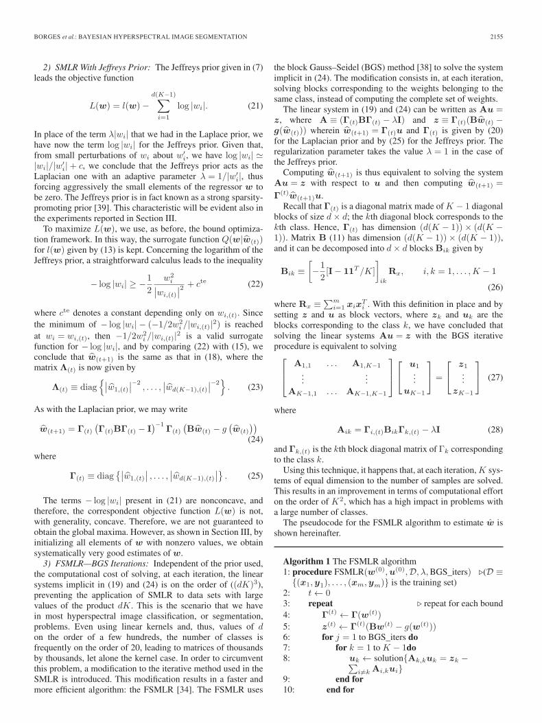
Algorithm 1 The FSMLR algorithm1: procedure FSMLR(w(0),u(0),D, λ,BGS_iters) �(D ≡{(x1,y1), . . . , (xm,ym)} is the training set)

2: t ← 03: repeat � repeat for each bound4: Γ(t) ← Γ(w(t))

5: z(t) ← Γ(t)(Bw(t) − g(w(t)))6: for j = 1 to BGS_iters do7: for k = 1 to K − 1do8: uk ← solution{Ak,kuk = zk −∑

i�=k Ai,kui}9: end for10: end for


11: t ← t+ 112: w(t) ← Γ(t)u13: until stopping criterion is satisfied.14: returnw(t)

15: end procedure

The gain introduced by the fast implementation of SMLRallows the optimization criteria used in the SMLR to be solved,which otherwise would not be possible in practice.

B. MLL Markov–Gibbs Prior

The application of FSMLR with a Laplacian or a Jeffreysprior enforces sparsity in the regressors parameterizing the pos-terior class probability distributions, providing a competitivemethod for the classification of hyperspectral images. However,the classifiers obtained can be improved by adding contextualspatial information modeling the piecewise smooth nature ofreal-world images.

In this paper, we adopt an MLL prior [40] to express contex-tual constraints in a principled manner. The MLL prior is anMRF that models the piecewise smooth nature of the imageelements, considering that adjacent class labels are likely tobelong to the same class [21].

The MLL prior model for segmentation has the formalstructure

p(y) =1

Zexp

(−

∑c∈C

Vc(y)

)(29)

where Z is a normalizing constant and the sum is over the so-called prior potentials Vc(y) for the set of cliques2 C over theimage, and

−Vc(y) =

⎧⎨⎩αyi

, if |c| = 1 (single clique)βc, if |c| >1 and ∀i,j∈cyi = yj−βc, if |c| > 1 and ∃i,j∈cyi �= yj

(30)

where βc is a nonnegative constant.In this paper, we assume that the cliques consist either of a

single pixel, i.e., c = {i}, for i ∈ S , or of a pair of neighboringpixels, i.e., c = {i, j}, where i, j ∈ S are first order neighbors.Furthermore, we set αk = α and βc = (1/2)β > 0, i.e., ourMLL gives no preference to any particular label or direction,and it is coherent with the assumption p(yi) = 1/K taken inthe beginning of Section II.

Let n1, n2, and n(y) denote the number of single-pixelcliques, the number of two-pixel cliques, and the number oftwo-pixel cliques with the same class label, respectively; then,(29) can be written as

p(y) =1

Zen1α− β

2 (n2−n(y))+ β2 n(y)

=1

Z ′ eβn(y) (31)

where Z ′ is a normalizing constant. It is therefore clear that theprior (31) attaches a higher likelihood to segmentations with alarge number of cliques having the same label. Given that, in the

2A clique is a set of pixels that are neighbors of one another.

present setting, n(y) =∑

{i,j}∈C δ(yi − yj), where δ denotesthe unit impulse function;3 then, the MLL prior can also bewritten as

p(y) =1

Z ′ eβ

∑{i,j}∈C

δ(yi−yj)

.

In the next section, we will exploit this formula for the MLLprior.

C. MAP Segmentation Using the α-Expansion Algorithm

After learning the class probability distributions p(x|y) ∝∏i p(yi|xi) with the FSMLR and modeling the prior over

classes p(y) with an MLL probability distribution, we aim atcomputing the MAP segmentation given by

y = argmaxy

p(x|y)p(y)

= argmaxy

∑i∈S

log p(yi|xi) + βn(y)

= argminy

∑i∈S

− log p(yi|xi)− β∑

{i,j}∈Cδ(yi − yj). (32)

The minimization of (32) is an integer optimization problem.The exact solution for K = 2 was introduced by mapping theproblem into the computation of a min-cut on a suitable graph[41]. This line of attack has been recently reintroduced andhas been intensely researched since then (see, e.g., [42]–[44]).The number of integer optimization problems that can nowbe solved exactly (or with a very good approximation) hasincreased substantially. The central concept in graph-cut-basedapproaches to integer optimization is the so-called submodular-ity of the pairwise terms: A pairwise term V (yi, yj) is said to besubmodular (or graph representable) if V (yi, yi) + V (yj , yj) ≤V (yi, yj) + V (yj , yi), for any yi, yj ∈ L. This is the case ofour binary term −δ(yi − yj). In this case, the α-expansionalgorithm [42] is applicable. It yields very good approximationsto the MAP segmentation problem and has, from the practicalpoint of view, an O(n) complexity.

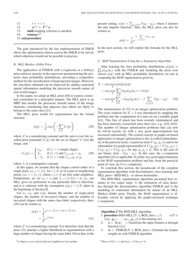
To conclude this section, the pseudocode of the completesegmentation algorithm with discriminative class learning andMLL prior—BSD-MLL—is shown hereinafter.

The BSD-MLL segmentation algorithm presented here re-sumes to two major steps: 1) the estimation of class densi-ties through the discriminative algorithm FSMLR and 2) themodeling of contextual information by means of an MLLMarkov–Gibbs prior. Finally, the MAP segmentation is ef-ficiently solved by applying the graph-cut-based techniqueα-expansion.

Algorithm 2 The BSD-MLL algorithm1: procedure BSD-MLL(D, λ,BGS_iters, c, β) �(D ≡

{(x1,y1), . . . , (xm,ym)} is the training set)2: x ← h(x) � Transform the input features x through

function h(x)3: w ← FSMLR(D, λ,BGS_iters) � Estimate the feature

weights w with FSMLR algorithm

3That is, δ(0) = 1, and δ(y) = 0 for y �= 0.


4: Edata(y) ← −∑n

i=1 log(p(yi|xi, w))5: Eprior(y) ← − log p(y)

6: Etrain(y) ←{0, if yi = yi (correct label)∞, if yi �= yi (incorrect label)

7: E(y) ← Edata(y) + Eprior(y) + Etrain(y) �Compute energy for all classes

8: y ← α-expansion(E(y)) � Minimization usingα-expansion algorithm.

9: returny10: end procedure

The first major step of the BSD-MLL algorithm is dom-inated by step 3, where the estimation of class densities isdone through the FSMLR algorithm. As seen in Section II-A3,this has a complexity O(kd3). The second major step of thesegmentation algorithm is dominated by step 8, where theα-expansion algorithm is used to determine the MAP segmenta-tion. This process has complexity O(n), as seen in Section II-C.In practice, we have therefore concluded that the complexity ofthe complete BSD-MLL algorithm is dominated by the FSMLRcomplexity O(kd3).

III. RESULTS

This section presents a series of experimental results with thefollowing main objectives.

1) Show the gains in segmentation accuracy due to theinclusion of the spatial prior information.

2) Compare the tradeoff between segmentation results andcomputational complexity obtained with the Laplacianand Jeffreys priors.

3) Compare the introduced BSD-MLL segmentation methodwith state-of-the-art competitors.

To meet these objectives, the BSD-MLL algorithm is appliedto simulated hyperspectral images and to the Indian Pines [45]and Pavia [46] benchmarked data sets. In the following sections,one for each data set, we start by analyzing the overall accuracy(OA) results from the FSMLR classifier, as well as the degreeof sparseness obtained with each prior, and then proceed withthe presentation of the OA segmentation results obtained withthe BSD-MLL segmentation method.

To evaluate the performance of the proposed method, we splitthe available complete ground-truth set, of size nT , into a train-ing set of size nL and a validation set of size nV = nT − nL.Then, we select subsets of size αnL (α ∈ {0.1, 0.2, 0.3, . . . , },i.e., 10%, 20%, 30%, . . . , of the complete training set). Eachreported OA is computed from ten Monte Carlo (MC) runs,where, in each run, αnL training samples are obtained byrandom sampling the full training set.

Owing to the sparsity enforcing priors we have adopted, onlya small number of components of the MLR are nonzero. Forthis reason and also because we are estimating the OAs basedon 10 MC runs, the OA estimates have very small errors. Forthis reason, we do not compute any other uncertainty statistics.

In Pavia Data set 1 experiments, we built training sets withthe same number of samples per class. This is, of course, notoptimal when the distribution of the class labels is nonuni-formly distributed because the training set does not account for

the class-label distribution. Anyway, we make the following re-marks: 1) The log posterior of the class labels is formally givenby (32) for any class-label distribution, which is a consequenceof the necessary compatibility between the MLL marginals andthe class-label distribution, and 2) in spite of the nonoptimalselection of the number of samples per class, we show belowstate-of-the-art performance in all experiments reported. Ofcourse, this issue is open to further research.

A. Simulated Data Sets

In this section, we report the results from two experiments:a binary classification/segmentation problem and a multiclassclassification/segmentation problem.

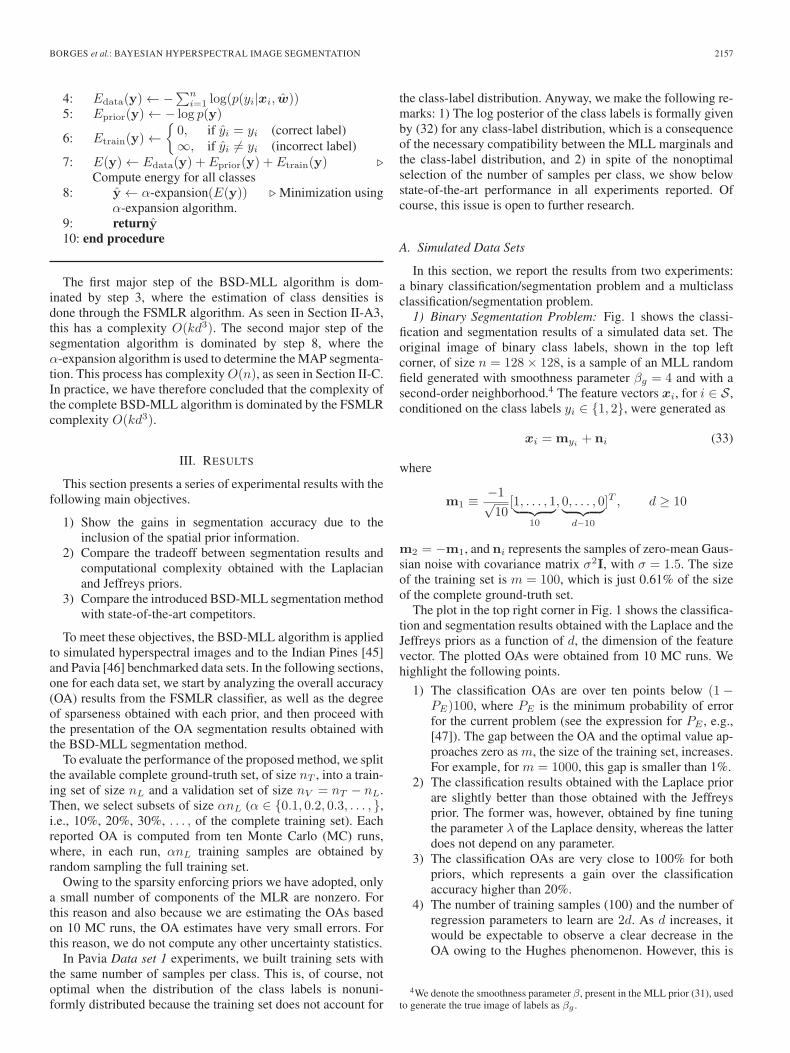
1) Binary Segmentation Problem: Fig. 1 shows the classi-fication and segmentation results of a simulated data set. Theoriginal image of binary class labels, shown in the top leftcorner, of size n = 128× 128, is a sample of an MLL randomfield generated with smoothness parameter βg = 4 and with asecond-order neighborhood.4 The feature vectors xi, for i ∈ S ,conditioned on the class labels yi ∈ {1, 2}, were generated as

xi = myi+ ni (33)

where

m1 ≡ −1√10

[1, . . . , 1︸︷︷︸10

, 0, . . . , 0︸︷︷︸d−10

]T , d ≥ 10

m2 = −m1, and ni represents the samples of zero-mean Gaus-sian noise with covariance matrix σ2I, with σ = 1.5. The sizeof the training set is m = 100, which is just 0.61% of the sizeof the complete ground-truth set.

The plot in the top right corner in Fig. 1 shows the classifica-tion and segmentation results obtained with the Laplace and theJeffreys priors as a function of d, the dimension of the featurevector. The plotted OAs were obtained from 10 MC runs. Wehighlight the following points.

1) The classification OAs are over ten points below (1−PE)100, where PE is the minimum probability of errorfor the current problem (see the expression for PE , e.g.,[47]). The gap between the OA and the optimal value ap-proaches zero as m, the size of the training set, increases.For example, for m = 1000, this gap is smaller than 1%.

2) The classification results obtained with the Laplace priorare slightly better than those obtained with the Jeffreysprior. The former was, however, obtained by fine tuningthe parameter λ of the Laplace density, whereas the latterdoes not depend on any parameter.

3) The classification OAs are very close to 100% for bothpriors, which represents a gain over the classificationaccuracy higher than 20%.

4) The number of training samples (100) and the number ofregression parameters to learn are 2d. As d increases, itwould be expectable to observe a clear decrease in theOA owing to the Hughes phenomenon. However, this is

4We denote the smoothness parameter β, present in the MLL prior (31), usedto generate the true image of labels as βg .


Fig. 1. (Top left) Sample of an MLL random field. (Top right) Classification and segmentation overall accuracies for Laplace and Jeffreys priors as a function ofd, the size of the feature vectors. (Bottom left) Vector of weights of the multilogistic regression for the Laplacian prior and for d = 100. (Bottom right) Vector ofweights of the multilogistic regression for the Jeffreys prior and for d = 100.

not the case, and the reason is the inclusion of sparsity-inducing priors controlling the machine complexity.

5) The effect of the Laplacian and Jeffreys sparsity-inducingpriors is to set most components of the regression vectorw to zero as shown in the bottom in Fig. 1; for d = 100,the use of the Laplacian prior yields 17 nonzeros out of100, whereas the use of the Jeffreys prior yields just 11nonzero components. This higher level of sparsity pro-moted by the Jeffreys prior has already been anticipatedand will be observed in all the results shown in thissection.

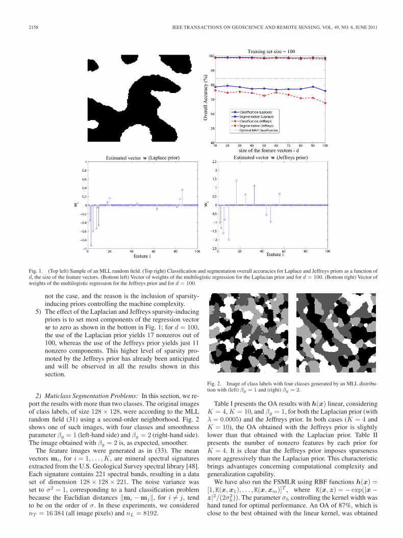
2) Muticlass Segmentation Problems: In this section, we re-port the results with more than two classes. The original imagesof class labels, of size 128× 128, were according to the MLLrandom field (31) using a second-order neighborhood. Fig. 2shows one of such images, with four classes and smoothnessparameter βg = 1 (left-hand side) and βg = 2 (right-hand side).The image obtained with βg = 2 is, as expected, smoother.

The feature images were generated as in (33). The meanvectors mi, for i = 1, . . . ,K, are mineral spectral signaturesextracted from the U.S. Geological Survey spectral library [48].Each signature contains 221 spectral bands, resulting in a dataset of dimension 128× 128× 221. The noise variance wasset to σ2 = 1, corresponding to a hard classification problembecause the Euclidian distances ‖mi −mj‖, for i �= j, tendto be on the order of σ. In these experiments, we considerednT = 16 384 (all image pixels) and nL = 8192.

Fig. 2. Image of class labels with four classes generated by an MLL distribu-tion with (left) βg = 1 and (right) βg = 2.

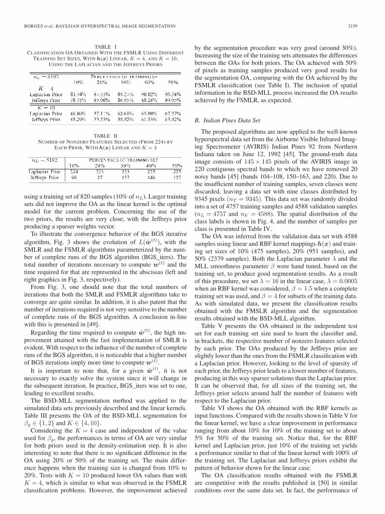
Table I presents the OA results with h(x) linear, consideringK = 4, K = 10, and βg = 1, for both the Laplacian prior (withλ = 0.0005) and the Jeffreys prior. In both cases (K = 4 andK = 10), the OA obtained with the Jeffreys prior is slightlylower than that obtained with the Laplacian prior. Table IIpresents the number of nonzero features by each prior forK = 4. It is clear that the Jeffreys prior imposes sparsenessmore aggressively than the Laplacian prior. This characteristicbrings advantages concerning computational complexity andgeneralization capability.

We have also run the FSMLR using RBF functions h(x) =[1, K(x,x1), . . . , K(x,xm)]T , where K(x, z) = − exp(|x−z|2/(2σ2

h)). The parameter σh controlling the kernel width washand tuned for optimal performance. An OA of 87%, which isclose to the best obtained with the linear kernel, was obtained


TABLE ICLASSIFICATION OA OBTAINED WITH THE FSMLR USING DIFFERENT

TRAINING SET SIZES, WITH h(x) LINEAR, K = 4, AND K = 10,USING THE LAPLACIAN AND THE JEFFREYS PRIORS

TABLE IINUMBER OF NONZERO FEATURES SELECTED (FROM 224) BY

EACH PRIOR, WITH h(x) LINEAR AND K = 4

using a training set of 820 samples (10% of nL). Larger trainingsets did not improve the OA as the linear kernel is the optimalmodel for the current problem. Concerning the use of thetwo priors, the results are very close, with the Jeffreys priorproducing a sparser weights vector.

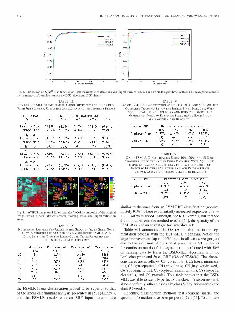
To illustrate the convergence behavior of the BGS iterativealgorithm, Fig. 3 shows the evolution of L(w(t)), with theSMLR and the FSMLR algorithms parameterized by the num-ber of complete runs of the BGS algorithm (BGS_iters). Thetotal number of iterations necessary to compute w(t) and thetime required for that are represented in the abscissas (left andright graphics in Fig. 3, respectively).

From Fig. 3, one should note that the total numbers ofiterations that both the SMLR and FSMLR algorithms take toconverge are quite similar. In addition, it is also patent that thenumber of iterations required is not very sensitive to the numberof complete runs of the BGS algorithm. A conclusion in-linewith this is presented in [49].

Regarding the time required to compute w(t), the high im-provement attained with the fast implementation of SMLR isevident. With respect to the influence of the number of completeruns of the BGS algorithm, it is noticeable that a higher numberof BGS iterations imply more time to compute w(t).

It is important to note that, for a given w(t), it is notnecessary to exactly solve the system since it will change inthe subsequent iteration. In practice, BGS_iters was set to one,leading to excellent results.

The BSD-MLL segmentation method was applied to thesimulated data sets previously described and the linear kernels.Table III presents the OA of the BSD-MLL segmentation forβg ∈ {1, 2} and K ∈ {4, 10}.

Considering the K = 4 case and independent of the valueused for βg , the performances in terms of OA are very similarfor both priors used in the density-estimation step. It is alsointeresting to note that there is no significant difference in theOA using 20% or 50% of the training set. The main differ-ence happens when the training size is changed from 10% to20%. Tests with K = 10 produced lower OA values than withK = 4, which is similar to what was observed in the FSMLRclassification problems. However, the improvement achieved

by the segmentation procedure was very good (around 30%).Increasing the size of the training sets attenuates the differencesbetween the OAs for both priors. The OA achieved with 50%of pixels as training samples produced very good results forthe segmentation OA, comparing with the OA achieved by theFSMLR classification (see Table I). The inclusion of spatialinformation in the BSD-MLL process increased the OA resultsachieved by the FSMLR, as expected.

B. Indian Pines Data Set

The proposed algorithms are now applied to the well-knownhyperspectral data set from the Airborne Visible Infrared Imag-ing Spectrometer (AVIRIS) Indian Pines 92 from NorthernIndiana taken on June 12, 1992 [45]. The ground-truth dataimage consists of 145× 145 pixels of the AVIRIS image in220 contiguous spectral bands to which we have removed 20noisy bands [45] (bands 104–108, 150–163, and 220). Due tothe insufficient number of training samples, seven classes werediscarded, leaving a data set with nine classes distributed by9345 pixels (nT = 9345). This data set was randomly dividedinto a set of 4757 training samples and 4588 validation samples(nL = 4757 and nV = 4588). The spatial distribution of theclass labels is shown in Fig. 4, and the number of samples perclass is presented in Table IV.

The OA was inferred from the validation data set with 4588samples using linear and RBF kernel mappings h(x) and train-ing set sizes of 10% (475 samples), 20% (951 samples), and50% (2379 samples). Both the Laplacian parameter λ and theMLL smoothness parameter β were hand tuned, based on thetraining set, to produce good segmentation results. As a resultof this procedure, we set λ = 16 in the linear case, λ = 0.0005when an RBF kernel was considered, β = 1.5 when a completetraining set was used, and β = 4 for subsets of the training data.As with simulated data, we present the classification resultsobtained with the FMSLR algorithm and the segmentationresults obtained with the BSD-MLL algorithm.

Table V presents the OA obtained in the independent testset for each training set size used to learn the classifier and,in brackets, the respective number of nonzero features selectedby each prior. The OAs produced by the Jeffreys prior areslightly lower than the ones from the FSMLR classification witha Laplacian prior. However, looking to the level of sparsity ofeach prior, the Jeffreys prior leads to a lower number of features,producing in this way sparser solutions than the Laplacian prior.It can be observed that, for all sizes of the training set, theJeffreys prior selects around half the number of features withrespect to the Laplacian prior.

Table VI shows the OA obtained with the RBF kernels asinput functions. Compared with the results shown in Table V forthe linear kernel, we have a clear improvement in performanceranging from about 10% for 10% of the training set to about5% for 50% of the training set. Notice that, for the RBFkernel and Laplacian prior, just 10% of the training set yieldsa performance similar to that of the linear kernel with 100% ofthe training set. The Laplacian and Jeffreys priors exhibit thepattern of behavior shown for the linear case.

The OA classification results obtained with the FSMLRare competitive with the results published in [50] in similarconditions over the same data set. In fact, the performance of


Fig. 3. Evolution of L(w(t)) as function of (left) the number of iterations and (right) time, for SMLR and FSMLR algorithms, with h(x) linear, parameterizedby the number of complete runs of the BGS algorithm (BGS_iters).

TABLE IIIOA OF BSD-MLL SEGMENTATION USING DIFFERENT TRAINING SETS,

WITH h(x) LINEAR, USING THE LAPLACIAN AND THE JEFFREYS PRIORS

Fig. 4. AVIRIS image used for testing: (Left) Color composite of the originalimage, which is near infrared, (center) training areas, and (right) validationareas.

TABLE IVNUMBER OF SAMPLES PER CLASS IN THE GROUND-TRUTH SETS. NOTE

THAT, ALTHOUGH THE NUMBER OF CLASSES IS THE SAME IN ALL

DATA SETS, THE TYPES OF LAND-COVER CLASS REPRESENTED

BY EACH CLASS ARE DIFFERENT

the FSMLR linear classification proved to be superior to thatof the linear discriminant analysis presented in [50] (82.32%),and the FSMLR results with an RBF input function are

TABLE VOA OF FSMLR CLASSIFICATION USING 10%, 20%, AND 50% AND THE

COMPLETE TRAINING SET OF THE INDIAN PINES DATA SET, WITH

h(x) LINEAR, USING LAPLACIAN AND JEFFREYS PRIORS. THE

NUMBER OF NONZERO FEATURES SELECTED BY EACH PRIOR

(OUT OF 200) IS IN BRACKETS

TABLE VIOA OF FSMLR CLASSIFICATION USING 10%, 20%, AND 50% OF

TRAINING SET OF THE INDIAN PINES DATA SET, WITH h(x) RBF,USING LAPLACIAN AND JEFFREYS PRIORS. THE NUMBER OF

NONZERO FEATURES SELECTED BY EACH PRIOR (OUT OF

475, 951, AND 2379, RESPECTIVELY) IS IN BRACKETS

similar to the ones from an SVM-RBF classification (approx-imately 91%), where exponentially increased sequences of σ =1, . . . , 50 were tested. Although, for RBF kernels, our methoddid not outperform the method used in [50], the sparsity of theFSMLR can be an advantage for large data sets.

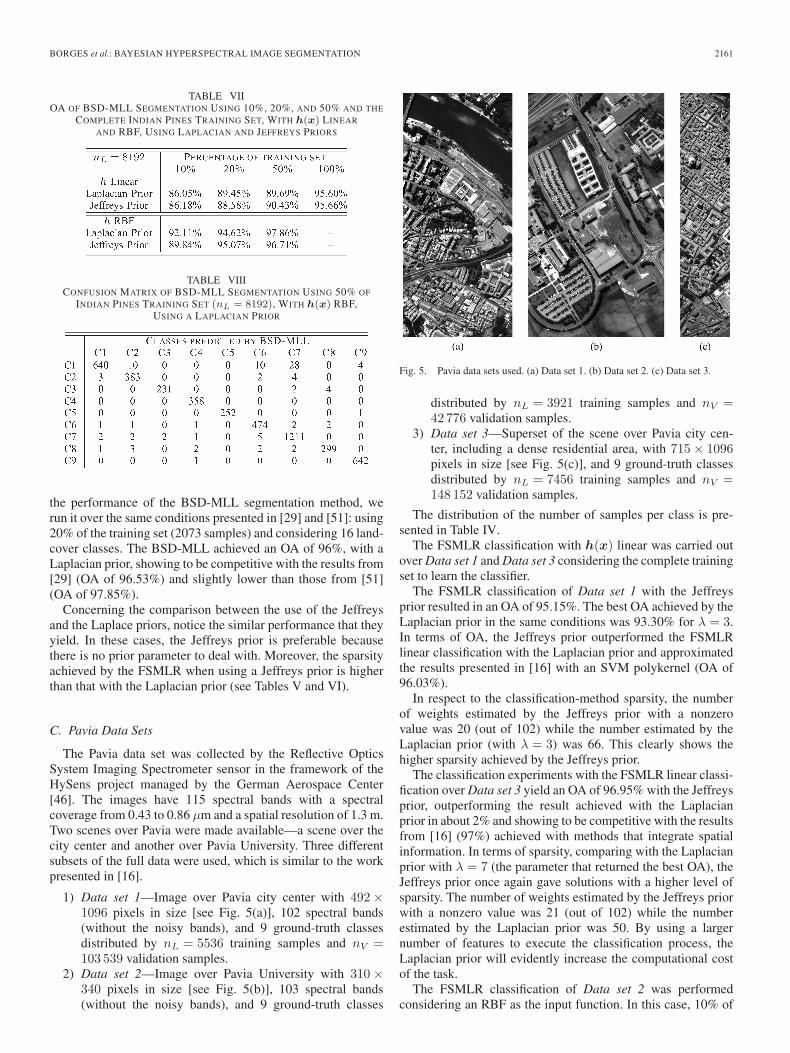
Table VII summarizes the OA results obtained in the seg-mentation process with the BSD-MLL algorithm. Notice thelarge improvement (up to 10%) that, in all cases, we got justdue to the inclusion of the spatial prior. Table VIII presentsthe confusion matrix of the segmentation performed with 50%of training data to learn the BSD-MLL algorithm with theLaplacian prior and h(x) RBF (OA of 97.86%). The classesconsidered are as follows: C1 (corn, no till), C2 (corn, minimumtill), C3 (grass/pasture), C4 (grass/trees), C5 (hay, windrowed),C6 (soybean, no till), C7 (soybean, minimum till), C8 (soybean,clean till), and C9 (woods). This table shows that the BSD-MLL was able to identify perfectly the class 4 (grass/trees) and,almost perfectly, other classes like class 5 (hay, windrowed) andclass 9 (woods).

Recently, classification methods that combine spatial andspectral information have been proposed [29], [51]. To compare


TABLE VIIOA OF BSD-MLL SEGMENTATION USING 10%, 20%, AND 50% AND THE

COMPLETE INDIAN PINES TRAINING SET, WITH h(x) LINEAR

AND RBF, USING LAPLACIAN AND JEFFREYS PRIORS

TABLE VIIICONFUSION MATRIX OF BSD-MLL SEGMENTATION USING 50% OF

INDIAN PINES TRAINING SET (nL = 8192), WITH h(x) RBF,USING A LAPLACIAN PRIOR

the performance of the BSD-MLL segmentation method, werun it over the same conditions presented in [29] and [51]: using20% of the training set (2073 samples) and considering 16 land-cover classes. The BSD-MLL achieved an OA of 96%, with aLaplacian prior, showing to be competitive with the results from[29] (OA of 96.53%) and slightly lower than those from [51](OA of 97.85%).

Concerning the comparison between the use of the Jeffreysand the Laplace priors, notice the similar performance that theyyield. In these cases, the Jeffreys prior is preferable becausethere is no prior parameter to deal with. Moreover, the sparsityachieved by the FSMLR when using a Jeffreys prior is higherthan that with the Laplacian prior (see Tables V and VI).

C. Pavia Data Sets

The Pavia data set was collected by the Reflective OpticsSystem Imaging Spectrometer sensor in the framework of theHySens project managed by the German Aerospace Center[46]. The images have 115 spectral bands with a spectralcoverage from 0.43 to 0.86 μm and a spatial resolution of 1.3 m.Two scenes over Pavia were made available—a scene over thecity center and another over Pavia University. Three differentsubsets of the full data were used, which is similar to the workpresented in [16].

1) Data set 1—Image over Pavia city center with 492×1096 pixels in size [see Fig. 5(a)], 102 spectral bands(without the noisy bands), and 9 ground-truth classesdistributed by nL = 5536 training samples and nV =103 539 validation samples.

2) Data set 2—Image over Pavia University with 310×340 pixels in size [see Fig. 5(b)], 103 spectral bands(without the noisy bands), and 9 ground-truth classes

Fig. 5. Pavia data sets used. (a) Data set 1. (b) Data set 2. (c) Data set 3.

distributed by nL = 3921 training samples and nV =42 776 validation samples.

3) Data set 3—Superset of the scene over Pavia city cen-ter, including a dense residential area, with 715× 1096pixels in size [see Fig. 5(c)], and 9 ground-truth classesdistributed by nL = 7456 training samples and nV =148 152 validation samples.

The distribution of the number of samples per class is pre-sented in Table IV.

The FSMLR classification with h(x) linear was carried outover Data set 1 and Data set 3 considering the complete trainingset to learn the classifier.

The FSMLR classification of Data set 1 with the Jeffreysprior resulted in an OA of 95.15%. The best OA achieved by theLaplacian prior in the same conditions was 93.30% for λ = 3.In terms of OA, the Jeffreys prior outperformed the FSMLRlinear classification with the Laplacian prior and approximatedthe results presented in [16] with an SVM polykernel (OA of96.03%).

In respect to the classification-method sparsity, the numberof weights estimated by the Jeffreys prior with a nonzerovalue was 20 (out of 102) while the number estimated by theLaplacian prior (with λ = 3) was 66. This clearly shows thehigher sparsity achieved by the Jeffreys prior.

The classification experiments with the FSMLR linear classi-fication over Data set 3 yield an OA of 96.95% with the Jeffreysprior, outperforming the result achieved with the Laplacianprior in about 2% and showing to be competitive with the resultsfrom [16] (97%) achieved with methods that integrate spatialinformation. In terms of sparsity, comparing with the Laplacianprior with λ = 7 (the parameter that returned the best OA), theJeffreys prior once again gave solutions with a higher level ofsparsity. The number of weights estimated by the Jeffreys priorwith a nonzero value was 21 (out of 102) while the numberestimated by the Laplacian prior was 50. By using a largernumber of features to execute the classification process, theLaplacian prior will evidently increase the computational costof the task.

The FSMLR classification of Data set 2 was performedconsidering an RBF as the input function. In this case, 10% of


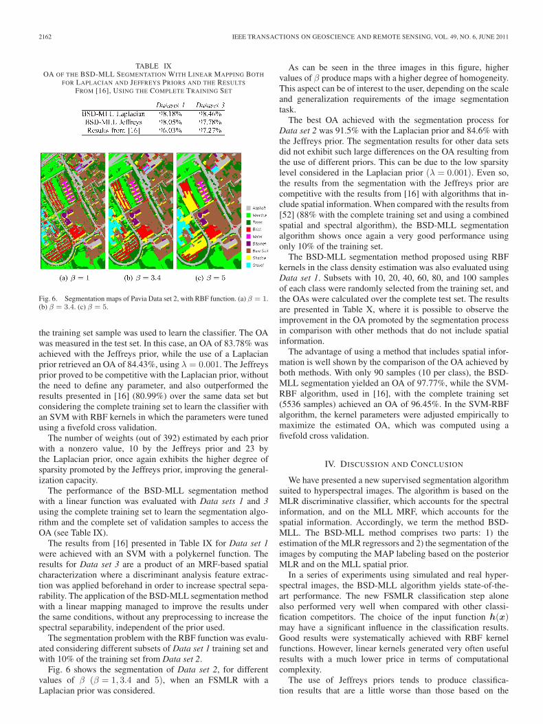
TABLE IXOA OF THE BSD-MLL SEGMENTATION WITH LINEAR MAPPING BOTH

FOR LAPLACIAN AND JEFFREYS PRIORS AND THE RESULTS

FROM [16], USING THE COMPLETE TRAINING SET

Fig. 6. Segmentation maps of Pavia Data set 2, with RBF function. (a) β = 1.(b) β = 3.4. (c) β = 5.

the training set sample was used to learn the classifier. The OAwas measured in the test set. In this case, an OA of 83.78% wasachieved with the Jeffreys prior, while the use of a Laplacianprior retrieved an OA of 84.43%, using λ = 0.001. The Jeffreysprior proved to be competitive with the Laplacian prior, withoutthe need to define any parameter, and also outperformed theresults presented in [16] (80.99%) over the same data set butconsidering the complete training set to learn the classifier withan SVM with RBF kernels in which the parameters were tunedusing a fivefold cross validation.

The number of weights (out of 392) estimated by each priorwith a nonzero value, 10 by the Jeffreys prior and 23 bythe Laplacian prior, once again exhibits the higher degree ofsparsity promoted by the Jeffreys prior, improving the general-ization capacity.

The performance of the BSD-MLL segmentation methodwith a linear function was evaluated with Data sets 1 and 3using the complete training set to learn the segmentation algo-rithm and the complete set of validation samples to access theOA (see Table IX).

The results from [16] presented in Table IX for Data set 1were achieved with an SVM with a polykernel function. Theresults for Data set 3 are a product of an MRF-based spatialcharacterization where a discriminant analysis feature extrac-tion was applied beforehand in order to increase spectral sepa-rability. The application of the BSD-MLL segmentation methodwith a linear mapping managed to improve the results underthe same conditions, without any preprocessing to increase thespectral separability, independent of the prior used.

The segmentation problem with the RBF function was evalu-ated considering different subsets of Data set 1 training set andwith 10% of the training set from Data set 2.

Fig. 6 shows the segmentation of Data set 2, for differentvalues of β (β = 1, 3.4 and 5), when an FSMLR with aLaplacian prior was considered.

As can be seen in the three images in this figure, highervalues of β produce maps with a higher degree of homogeneity.This aspect can be of interest to the user, depending on the scaleand generalization requirements of the image segmentationtask.

The best OA achieved with the segmentation process forData set 2 was 91.5% with the Laplacian prior and 84.6% withthe Jeffreys prior. The segmentation results for other data setsdid not exhibit such large differences on the OA resulting fromthe use of different priors. This can be due to the low sparsitylevel considered in the Laplacian prior (λ = 0.001). Even so,the results from the segmentation with the Jeffreys prior arecompetitive with the results from [16] with algorithms that in-clude spatial information. When compared with the results from[52] (88% with the complete training set and using a combinedspatial and spectral algorithm), the BSD-MLL segmentationalgorithm shows once again a very good performance usingonly 10% of the training set.

The BSD-MLL segmentation method proposed using RBFkernels in the class density estimation was also evaluated usingData set 1. Subsets with 10, 20, 40, 60, 80, and 100 samplesof each class were randomly selected from the training set, andthe OAs were calculated over the complete test set. The resultsare presented in Table X, where it is possible to observe theimprovement in the OA promoted by the segmentation processin comparison with other methods that do not include spatialinformation.

The advantage of using a method that includes spatial infor-mation is well shown by the comparison of the OA achieved byboth methods. With only 90 samples (10 per class), the BSD-MLL segmentation yielded an OA of 97.77%, while the SVM-RBF algorithm, used in [16], with the complete training set(5536 samples) achieved an OA of 96.45%. In the SVM-RBFalgorithm, the kernel parameters were adjusted empirically tomaximize the estimated OA, which was computed using afivefold cross validation.

IV. DISCUSSION AND CONCLUSION

We have presented a new supervised segmentation algorithmsuited to hyperspectral images. The algorithm is based on theMLR discriminative classifier, which accounts for the spectralinformation, and on the MLL MRF, which accounts for thespatial information. Accordingly, we term the method BSD-MLL. The BSD-MLL method comprises two parts: 1) theestimation of the MLR regressors and 2) the segmentation of theimages by computing the MAP labeling based on the posteriorMLR and on the MLL spatial prior.

In a series of experiments using simulated and real hyper-spectral images, the BSD-MLL algorithm yields state-of-the-art performance. The new FSMLR classification step alonealso performed very well when compared with other classi-fication competitors. The choice of the input function h(x)may have a significant influence in the classification results.Good results were systematically achieved with RBF kernelfunctions. However, linear kernels generated very often usefulresults with a much lower price in terms of computationalcomplexity.

The use of Jeffreys priors tends to produce classifica-tion results that are a little worse than those based on the


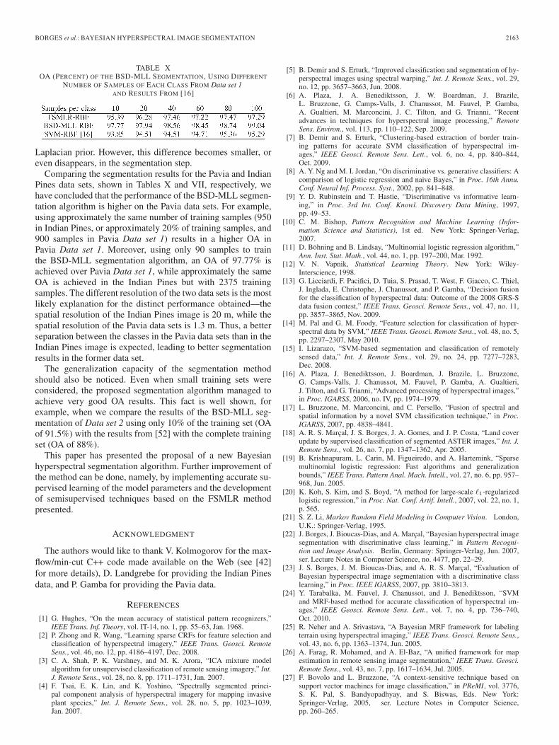
TABLE XOA (PERCENT) OF THE BSD-MLL SEGMENTATION, USING DIFFERENT

NUMBER OF SAMPLES OF EACH CLASS FROM Data set 1AND RESULTS FROM [16]

Laplacian prior. However, this difference becomes smaller, oreven disappears, in the segmentation step.

Comparing the segmentation results for the Pavia and IndianPines data sets, shown in Tables X and VII, respectively, wehave concluded that the performance of the BSD-MLL segmen-tation algorithm is higher on the Pavia data sets. For example,using approximately the same number of training samples (950in Indian Pines, or approximately 20% of training samples, and900 samples in Pavia Data set 1) results in a higher OA inPavia Data set 1. Moreover, using only 90 samples to trainthe BSD-MLL segmentation algorithm, an OA of 97.77% isachieved over Pavia Data set 1, while approximately the sameOA is achieved in the Indian Pines but with 2375 trainingsamples. The different resolution of the two data sets is the mostlikely explanation for the distinct performance obtained—thespatial resolution of the Indian Pines image is 20 m, while thespatial resolution of the Pavia data sets is 1.3 m. Thus, a betterseparation between the classes in the Pavia data sets than in theIndian Pines image is expected, leading to better segmentationresults in the former data set.

The generalization capacity of the segmentation methodshould also be noticed. Even when small training sets wereconsidered, the proposed segmentation algorithm managed toachieve very good OA results. This fact is well shown, forexample, when we compare the results of the BSD-MLL seg-mentation of Data set 2 using only 10% of the training set (OAof 91.5%) with the results from [52] with the complete trainingset (OA of 88%).

This paper has presented the proposal of a new Bayesianhyperspectral segmentation algorithm. Further improvement ofthe method can be done, namely, by implementing accurate su-pervised learning of the model parameters and the developmentof semisupervised techniques based on the FSMLR methodpresented.

ACKNOWLEDGMENT

The authors would like to thank V. Kolmogorov for the max-flow/min-cut C++ code made available on the Web (see [42]for more details), D. Landgrebe for providing the Indian Pinesdata, and P. Gamba for providing the Pavia data.

REFERENCES

[1] G. Hughes, “On the mean accuracy of statistical pattern recognizers,”IEEE Trans. Inf. Theory, vol. IT-14, no. 1, pp. 55–63, Jan. 1968.

[2] P. Zhong and R. Wang, “Learning sparse CRFs for feature selection andclassification of hyperspectral imagery,” IEEE Trans. Geosci. RemoteSens., vol. 46, no. 12, pp. 4186–4197, Dec. 2008.

[3] C. A. Shah, P. K. Varshney, and M. K. Arora, “ICA mixture modelalgorithm for unsupervised classification of remote sensing imagery,” Int.J. Remote Sens., vol. 28, no. 8, pp. 1711–1731, Jan. 2007.

[4] F. Tsai, E. K. Lin, and K. Yoshino, “Spectrally segmented princi-pal component analysis of hyperspectral imagery for mapping invasiveplant species,” Int. J. Remote Sens., vol. 28, no. 5, pp. 1023–1039,Jan. 2007.

[5] B. Demir and S. Erturk, “Improved classification and segmentation of hy-perspectral images using spectral warping,” Int. J. Remote Sens., vol. 29,no. 12, pp. 3657–3663, Jun. 2008.

[6] A. Plaza, J. A. Benediktsson, J. W. Boardman, J. Brazile,L. Bruzzone, G. Camps-Valls, J. Chanussot, M. Fauvel, P. Gamba,A. Gualtieri, M. Marconcini, J. C. Tilton, and G. Trianni, “Recentadvances in techniques for hyperspectral image processing,” RemoteSens. Environ., vol. 113, pp. 110–122, Sep. 2009.

[7] B. Demir and S. Erturk, “Clustering-based extraction of border train-ing patterns for accurate SVM classification of hyperspectral im-ages,” IEEE Geosci. Remote Sens. Lett., vol. 6, no. 4, pp. 840–844,Oct. 2009.

[8] A. Y. Ng and M. I. Jordan, “On discriminative vs. generative classifiers: Acomparison of logistic regression and naive Bayes,” in Proc. 16th Annu.Conf. Neural Inf. Process. Syst., 2002, pp. 841–848.

[9] Y. D. Rubinstein and T. Hastie, “Discriminative vs informative learn-ing,” in Proc. 3rd Int. Conf. Knowl. Discovery Data Mining, 1997,pp. 49–53.

[10] C. M. Bishop, Pattern Recognition and Machine Learning (Infor-mation Science and Statistics), 1st ed. New York: Springer-Verlag,2007.

[11] D. Böhning and B. Lindsay, “Multinomial logistic regression algorithm,”Ann. Inst. Stat. Math., vol. 44, no. 1, pp. 197–200, Mar. 1992.

[12] V. N. Vapnik, Statistical Learning Theory. New York: Wiley-Interscience, 1998.

[13] G. Licciardi, F. Pacifici, D. Tuia, S. Prasad, T. West, F. Giacco, C. Thiel,J. Inglada, E. Christophe, J. Chanussot, and P. Gamba, “Decision fusionfor the classification of hyperspectral data: Outcome of the 2008 GRS-Sdata fusion contest,” IEEE Trans. Geosci. Remote Sens., vol. 47, no. 11,pp. 3857–3865, Nov. 2009.

[14] M. Pal and G. M. Foody, “Feature selection for classification of hyper-spectral data by SVM,” IEEE Trans. Geosci. Remote Sens., vol. 48, no. 5,pp. 2297–2307, May 2010.

[15] I. Lizarazo, “SVM-based segmentation and classification of remotelysensed data,” Int. J. Remote Sens., vol. 29, no. 24, pp. 7277–7283,Dec. 2008.

[16] A. Plaza, J. Benediktsson, J. Boardman, J. Brazile, L. Bruzzone,G. Camps-Valls, J. Chanussot, M. Fauvel, P. Gamba, A. Gualtieri,J. Tilton, and G. Trianni, “Advanced processing of hyperspectral images,”in Proc. IGARSS, 2006, no. IV, pp. 1974–1979.

[17] L. Bruzzone, M. Marconcini, and C. Persello, “Fusion of spectral andspatial information by a novel SVM classification technique,” in Proc.IGARSS, 2007, pp. 4838–4841.

[18] A. R. S. Marçal, J. S. Borges, J. A. Gomes, and J. P. Costa, “Land coverupdate by supervised classification of segmented ASTER images,” Int. J.Remote Sens., vol. 26, no. 7, pp. 1347–1362, Apr. 2005.

[19] B. Krishnapuram, L. Carin, M. Figueiredo, and A. Hartemink, “Sparsemultinomial logistic regression: Fast algorithms and generalizationbounds,” IEEE Trans. Pattern Anal. Mach. Intell., vol. 27, no. 6, pp. 957–968, Jun. 2005.

[20] K. Koh, S. Kim, and S. Boyd, “A method for large-scale �1-regularizedlogistic regression,” in Proc. Nat. Conf. Artif. Intell., 2007, vol. 22, no. 1,p. 565.

[21] S. Z. Li, Markov Random Field Modeling in Computer Vision. London,U.K.: Springer-Verlag, 1995.

[22] J. Borges, J. Bioucas-Dias, and A. Marçal, “Bayesian hyperspectral imagesegmentation with discriminative class learning,” in Pattern Recogni-tion and Image Analysis. Berlin, Germany: Springer-Verlag, Jun. 2007,ser. Lecture Notes in Computer Science, no. 4477, pp. 22–29.

[23] J. S. Borges, J. M. Bioucas-Dias, and A. R. S. Marçal, “Evaluation ofBayesian hyperspectral image segmentation with a discriminative classlearning,” in Proc. IEEE IGARSS, 2007, pp. 3810–3813.

[24] Y. Tarabalka, M. Fauvel, J. Chanussot, and J. Benediktsson, “SVMand MRF-based method for accurate classification of hyperspectral im-ages,” IEEE Geosci. Remote Sens. Lett., vol. 7, no. 4, pp. 736–740,Oct. 2010.

[25] R. Neher and A. Srivastava, “A Bayesian MRF framework for labelingterrain using hyperspectral imaging,” IEEE Trans. Geosci. Remote Sens.,vol. 43, no. 6, pp. 1363–1374, Jun. 2005.

[26] A. Farag, R. Mohamed, and A. El-Baz, “A unified framework for mapestimation in remote sensing image segmentation,” IEEE Trans. Geosci.Remote Sens., vol. 43, no. 7, pp. 1617–1634, Jul. 2005.

[27] F. Bovolo and L. Bruzzone, “A context-sensitive technique based onsupport vector machines for image classification,” in PReMI, vol. 3776,S. K. Pal, S. Bandyopadhyay, and S. Biswas, Eds. New York:Springer-Verlag, 2005, ser. Lecture Notes in Computer Science,pp. 260–265.


[28] D. Liu, M. Kelly, and P. Gong, “A spatial-temporal approach to mon-itoring forest disease spread using multi-temporal high spatial resolu-tion imagery,” Remote Sens. Environ., vol. 101, no. 2, pp. 167–180,Mar. 2006.

[29] G. Camps-Valls, L. Gomez-Chova, J. Munoz-Mari, J. Vila-Frances, andJ. Calpe-Maravilla, “Composite kernels for hyperspectral image classi-fication,” IEEE Geosci. Remote Sens. Lett., vol. 3, no. 1, pp. 93–97,Jan. 2006.

[30] Y. Tarabalka, J. Chanussot, and J. Benediktsson, “Segmentation and clas-sification of hyperspectral images using watershed transformation,” Pat-tern Recognit., vol. 43, no. 7, pp. 2367–2379, Jul. 2010.

[31] Y. Tarabalka, J. Chanussot, and J. A. Benediktsson, “Segmentation andclassification of hyperspectral images using minimum spanning forestgrown from automatically selected markers,” IEEE Trans. Syst., Man,Cybern. B, Cybern., vol. 40, no. 5, pp. 1267–1279, Oct. 2010.

[32] H. Jeffreys, “An invariant form for the prior probability in estimationproblems,” Proc. R. Soc. Lond. A, Math. Phys. Sci., vol. 186, no. 1007,pp. 453–461, Sep. 1946.

[33] Y. Boykov, O. Veksler, and R. Zabih, “Fast approximate energy minimiza-tion via graph cuts,” IEEE Trans. Pattern Anal. Mach. Intell., vol. 23,no. 11, pp. 1222–1239, Nov. 2001.

[34] J. Borges, J. Bioucas-Dias, and A. Marçal, “Fast sparse multinomial re-gression applied to hyperspectral data,” in Image Analysis and Recogni-tion. Berlin, Germany: Springer-Verlag, Sep. 2006, ser. Lecture Notesin Computer Science, no. 4142, pp. 700–709.

[35] G. McLachlan, Discriminant Analysis and Statistical Pattern Recognition.New York: Wiley, 1992, ser. Probability and Mathematical Statistics.Applied Probability and Statistics.

[36] T. Hastie, R. Tibshirani, and J. Friedman, The Elements of StatisticalLearning—Data Mining, Inference and Prediction. New York: Springer-Verlag, 2001, ser. Springer Series in Statistics.

[37] K. Lange, Optimization. New York: Springer-Verlag, 2004,ser. Springer Texts in Statistics.

[38] A. Quarteroni, R. Sacco, and F. Saleri, Numerical Mathematics.New York: Springer-Verlag, 2000, ser. TAM 37.

[39] M. Figueiredo, “Adaptative sparseness using Jeffreys prior,” in Advancesin Neural Network Information Processing Systems 14. Cambridge, MA:MIT Press, 2001, pp. 697–704.

[40] S. Geman and D. Geman, “Stochastic relaxation, Gibbs distribution, andthe Bayesian restoration of images,” IEEE Trans. Pattern Anal. Mach.Intell., vol. PAMI-6, no. 6, pp. 721–741, Nov. 1984.

[41] D. M. Greig, B. T. Porteous, and A. H. Seheult, “Exact maximum aposteriori estimation for binary images,” J. R. Stat. Soc. B, vol. 51, no. 2,pp. 271–279, 1989.

[42] Y. Boykov and V. Kolmogorov, “An experimental comparison ofmincut/max-flow algorithms for energy minimization in vision,” IEEETrans. Pattern Anal. Mach. Intell., vol. 26, no. 9, pp. 1124–1137,Sep. 2004.

[43] V. Kolmogorov and R. Zabin, “What energy functions can be minimizedvia graph cuts?” IEEE Trans. Pattern Anal. Mach. Intell., vol. 26, no. 2,pp. 147–159, Feb. 2004.

[44] E. Boros, P. L. Hammer, R. Sun, and G. Tavares, “A max-flow approach toimproved lower bounds for quadratic unconstrained binary optimization(QUBO),” Discr. Optim., vol. 5, no. 2, pp. 501–529, 2008.

[45] D. Landgrebe, Signal Theory Methods in Multispectral Remote Sensing.Hoboken, NJ: Wiley, 2003.

[46] F. Dell’Acqua, P. Gamba, A. Ferrari, J. Palmason, J. Benediktsson, andK. Arnason, “Exploiting spectral and spatial information in hyperspectralurban data with high resolution,” IEEE Geosci. Remote Sens. Lett., vol. 1,no. 4, pp. 322–326, Oct. 2004.

[47] R. Duda, P. Hart, and D. Stork, Pattern Classification. New York: Wiley-Interscience, 2001.

[48] USGS, USGS Spectroscopy Lab. U.S. Geological Survey, 2006. [Online].Available: http://speclab.cr.usgs.gov/

[49] J. Bioucas-Dias, “Bayesian wavelet-based image deconvolution: A GEMalgorithm exploiting a class of heavy-tailed priors,” IEEE Trans. ImageProcess., vol. 15, no. 4, pp. 937–951, Apr. 2006.

[50] G. Camps-Valls and L. Bruzzone, “Kernel-based methods for hyperspec-tral image classification,” IEEE Trans. Geosci. Remote Sens., vol. 43,no. 6, pp. 1351–1362, Jun. 2005.

[51] S. Velasco-Forero and V. Manian, “Improving hyperspectral image clas-sification using spatial preprocessing,” IEEE Geosci. Remote Sens. Lett.,vol. 6, no. 2, pp. 297–301, Apr. 2009.

[52] M. Fauvel, J. Chanussot, J. Benediktsson, and J. Sveinsson, “Spectral andspatial classification of hyperspectral data using SVMs and morphologicalprofiles,” IEEE Trans. Geosci. Remote Sens., vol. 46, no. 11, pp. 3804–3814, Nov. 2008.

Janete S. Borges received the B.Sc. degree in math-ematics applied to technology, the M.Sc. degree instatistics, and the Ph.D. degree in interdisciplinarysciences from the Universidade do Porto, Porto,Portugal, in 2001, 2003, and 2009, respectively.

From 2001 to 2009, she was a Researcher withCentro de Investigação em Ciências Geo-Espaciais,Faculdade de Ciências, Universidade do Porto,where she participated in several R&D projects.Since 2010, she has been a Postdoctoral Fellow withInstituto de Engenharia de Sistemas e Computadores

do Porto. She is also currently an Assistant Professor with the Instituto Superiorda Maia, Maia, Portugal. Her scientific interests include image classification,pattern recognition, and remote sensing.

José M. Bioucas-Dias (S’87–M’95) received theE.E., M.Sc., Ph.D., and “Agregado” degrees inelectrical and computer engineering from InstitutoSuperior Técnico (IST), Universidade Técnica deLisboa, Lisboa, Portugal, in 1985, 1991, 1995, and2007, respectively.

Since 1995, he has been with the Departamento deEngenharia Electrotécnica e de Computadores, IST.He is also a Senior Researcher with the Communi-cation Theory and Pattern Recognition Group, Insti-tuto de Telecomunicações, Universidade Técnica de

Lisboa, which is a private not-for-profit research institution. He is involved inseveral national and international research projects and networks, includingthe Marie Curie Actions Hyperspectral Imaging Network and the EuropeanDoctoral Program in Signal Processing. His scientific interests include signaland image processing, pattern recognition, optimization, and remote sensing.

Dr. Bioucas-Dias has been a member of program/technical committees ofseveral international conferences, including Conference on Computer Visionand Pattern Recognition, International Conference on Pattern Recognition,International Conference on Image Analysis and Recognition, InternationalGeoscience and Remote Sensing Symposium, International Conference onImage Processing, SPIE, Energy Minimization Methods in Computer Visionand Pattern Recognition, International Symposium on Visual Computing, andWorkshop on Hyperspectral Image and Signal Processing: Evolution in RemoteSensing. He was an Associate Editor of the IEEE TRANSACTIONS ON CIR-CUITS AND SYSTEMS and is an Associate Editor of the IEEE TRANSACTIONS

ON IMAGE PROCESSING and a Guest Editor of a special issue of the IEEETRANSACTIONS ON GEOSCIENCE AND REMOTE SENSING.

Andre R. S. Marcal received the B.Sc. degree inphysics (solid-state physics) from the Universidadedo Porto, Porto, Portugal, in 1991 and the M.Sc.and Ph.D. degrees in remote sensing and imageprocessing from the University of Dundee, Dundee,Scotland, in 1994 and 1998, respectively.

He is currently an Assistant Professor with theDepartamento de Matemática Aplicada, Faculdadede Ciências, Universidade do Porto. His researchinterests include various topics in remote sensing andimage processing.

Dr. Marcal was a bureau member, Secretary General, and Vice-Chairman ofthe European Association of Remote Sensing Laboratories from 2005 to 2010.He was a recipient of the prize for the best Ph.D. from the Remote SensingSociety (U.K.) in 1999.

Bayesian Hyperspectral Image Segmentation With ...bioucas/files/ieee_tgars_2011_fsmlr.pdf · IEEE...

Documents

Transcript of Bayesian Hyperspectral Image Segmentation With ...bioucas/files/ieee_tgars_2011_fsmlr.pdf · IEEE...