Contents lists available at SciVerse ScienceDirect

Journal of Sound and Vibration

Journal of Sound and Vibration 331 (2012) 798–814

0022-46

doi:10.1

n Corr

E-m

journal homepage: www.elsevier.com/locate/jsvi

Bayesian force reconstruction with an uncertain model

E. Zhang a,n, J. Antoni b, P. Feissel a

a Roberval Laboratory of Mechanics, CNRS UMR 6253, University of Technology of Compi�egne, Franceb Vibration and Acoustic Laboratory, University of Lyon, F-69621 Villeurbanne, France

a r t i c l e i n f o

Article history:

Received 22 December 2010

Received in revised form

18 September 2011

Accepted 16 October 2011

Handling Editor: K. Wordenmodel uncertainty and the regularization parameter are jointly determined with the

Available online 26 October 2011

0X/$ - see front matter & 2011 Elsevier Ltd.

016/j.jsv.2011.10.021

esponding author.

ail address: erliang.zhang@utc.fr (E. Zhang).

a b s t r a c t

This paper presents a Bayesian approach for force reconstruction which can deal with

both measurement noise and model uncertainty. In particular, an uncertain model is

considered for inversion in the form of a matrix of frequency response functions whose

modal parameters originate from either measurements or a finite element model. The

unknown force through Monte Carlo Markov chain methods. Bayesian credible intervals

of the force are built from its posterior probability density function by taking into

account the quantified model uncertainty and measurement noise. The proposed

approach is illustrated and validated on numerical and experimental examples.

& 2011 Elsevier Ltd. All rights reserved.

1. Introduction

The knowledge of the force exerted on a mechanical system is an important information in many structural dynamicapplications. However, its measurement with transducers is a difficult task in many instances, especially if the measurement isintrusive or if the force is distributed. Instead, vibration responses can be conveniently measured. It is the reason why indirectmethods are often preferred, which consist in reconstructing forces based on inverting the model of a mechanical system.In recent years, various model-based force reconstruction methods have been proposed, especially within the context ofaccurate models (modal model, impulse response function or frequency response function, FRF) [1–8]. Much attention has beenpaid on the stability of the inversion, for instance by means of the singular value decomposition or the Tikhonov regularizationmethod [3–5]. Antoni [1] illustrates an optimal inverse filter to reconstruct the cylinder pressures of IC engines. Choi [6]compares the performance of the ordinary and generalized cross validation methods and the L-curve criterion in selecting theoptimal parameter for Tikhonov regularization. The Kalman filter along with a recursive least-squares algorithm is adopted forthe online force reconstruction based on a finite element (FE) model [7]. Gunawan [8] uses a two-step B-splines method toapproximate and to regularize an impact-force profile. Besides, attention is also paid to the reconstruction of distributed forcebased on a modal model in [9,10] using Thikonov regularization and in [11] using mode selection method.

As a matter of fact, the final reconstructed force heavily relies on the quality of the modal model or the FRFs which areinverted and are typically either estimated from experimental modal analysis [12,13] or predicted by a FE model. By virtueof its predictive ability, the FE approach is surely promising in model-based force reconstruction provided a modelupdating stage [14] is performed before inversion. Nevertheless, even a finely updated model cannot reproduce exactly thereal behavior of a structure due to limitations of the model itself. In addition, no matter how precisely a structure’s FRFsare measured in the laboratory, these will never correspond perfectly to the actual operating FRFs due to changes in the

All rights reserved.

E. Zhang et al. / Journal of Sound and Vibration 331 (2012) 798–814 799

boundary conditions and damping mechanisms when passing from the laboratory environment to practical operatingstate. As far as the authors know, these aspects have seldom been taken into account in force reconstruction problemsdespite their importance. A total least-square scheme is used to address the errors associated with the FRF matrix in [5].Similarly Ref. [15] proposes a discrete modal filter to reduce the error propagation from the biased modal parameters tothe reconstructed force.

On account of the presence of measurement noise and modeling error, force reconstruction is tackled within a probabilisticframework. Since measurement noise is inherently aleatory because of nature, and modeling error can be considered asrandom by epistemic uncertainty due to lack of knowledge, the model error is hereafter called model uncertainty and isconsidered within a probabilistic context. In the present work, force reconstruction is particularly investigated from a Bayesianperspective by viewing the unknown quantities as random variables or stochastic process [16,17]. This has several advantages.First it endows the unknown force with prior information on the possible range of its values in the form of a probability densityfunction (p.d.f.), which naturally imposes an intrinsic regularization. Second, the Bayesian approach furnishes a rigorousprobabilistic framework to account for all possible sources of errors that participate to the uncertainty of the reconstructedforce, including the measurement noise and the model uncertainty. As an original contribution, the model uncertainty isconsidered by following two strategies, firstly encoded at the FRFs level, then at the level of the modal parameters. The firststrategy is the simplest, but the second one is found superior when the forward model happens to have a significant level ofuncertainty in a certain frequency band. In both cases, Bayesian reconstructions are established for reconstructing the force andjointly quantifying the measurement noise and model uncertainty through Monte Carlo Markov chain (MCMC) methods.Bayesian credible interval on the reconstructed force is systematically delivered, which is of practical use.

The rest of paper is organized as follows. Section 2 introduces some generalities on the force reconstruction algorithmwithin the Bayesian framework. Section 3 proposes a general Bayesian formulation based on MCMC implementation toreconstruct forces by inverting uncertain FRFs and discusses the role of local regularization. Section 4 proposes a similarapproach when reconstruction is carried out under uncertain modal parameters. Finally, Section 5 illustrates the proposedapproaches on numerical and experimental examples and conclusions are given in Section 6.

2. Force reconstruction within the Bayesian framework

In this paper, an italic character means a scalar variable, a bold character denotes a vector, and a matrix is expressed bya character enclosed in a bracket. The model-based approach consists in reconstructing the force from measurementsbased on the physical model of a mechanical system. A system excited by only one force and returning ns outputs isconsidered here for simplicity, the generalization to the multi-force case being quite straightforward. Thus, the input–output relation in a frequency band is

YðoÞ ¼HðoÞFðoÞþNðoÞ, olrorou (1)

with YðoÞ 2 Cns the column vector of the ns measured responses (e.g. accelerations) at frequency o, FðoÞ 2 C the force,HðoÞ 2 Cns the vector of FRFs at frequency o between the positions of the ns measured outputs and the position of theforce, and NðoÞ 2 Cns the vector of the measurement noises. For a linear time-invariant system, the k-th generic element inthe vector of HðoÞ is expressed as

Hkðo;aÞ ¼Xmr ¼ 1

�o2Ark

o2r�o2þ2Eoroxr

, (2)

where E¼ffiffiffiffiffiffiffi�1p

and where the natural frequencies for ,r¼ 1, . . . ,mg, the damping ratios fxr ,r¼ 1, . . . ,mg and all the modalresidues fArk,r¼ 1, . . . ,m; k¼ 1, . . . ,nsg are concatenated in vector a. The values of the modal parameters are typicallyreturned by an updated FE model or experimental modal analysis; however, this is always to a limited degree of accuracydue to modeling or experimental errors and the fact that the real system is always more or less nonlinear. As a result, anadditional term should be added in Eq. (1) to include explicitly the model uncertainty (nonlinear distortions, systematicerror) in addition to measurement noise, which will be discussed later.

As emphasized in the Introduction, the Bayesian approach allows for the propagation and quantification of the errors onthe reconstructed force by delivering a posterior probability distribution. Denoting by x the vector collecting the unknownparameters (force þ measurement noise þ model uncertainty), its joint posterior p.d.f. is obtained from Bayes’ rule as

pðx9DÞ ¼ pð½Y �9xÞpðx9I Þ=pðDÞ, (3)

where the matrix ½Y� 2 Cno�ns collects the ns measured outputs at no discrete frequencies in the frequency band of interest½ol,ou�, I is introduced to make explicit the prior information, and D is the union set of the prior information I andexperimental information ½Y �. The elements in Eq. (3) are listed as follows:

�

the so-called likelihood function, pð½Y �9xÞ, which reflects the probability of observing the data [Y] given a set ofparameters x; � the prior p.d.f., pðx9I Þ, which reflects our knowledge on the parameters before experiments are undertaken. If x is well

known, it is represented by a narrow p.d.f., otherwise by a flat one;

E. Zhang et al. / Journal of Sound and Vibration 331 (2012) 798–814800

�

the evidence function pðDÞ ¼R

pð½Y �9xÞpðx9I Þ dx, which is usually used for the model class selection and is independentof the model parameters.

The construction of the likelihood implies two steps, one is the characterization of the measurement noise, the other is therepresentation of the model uncertainty. According to the central limit theorem, the measurement noise in the frequencydomain is asymptotically a zero-mean circular normal complex random variable with independent values over frequency[18,19]. The circular normal complex distribution N c is illustrated in Appendix A. For instance, the measurement noiserelated to the k-th response,

NkðoÞ �N cð0,s2NÞ (4)

with s2N an unknown hyper-parameter to be determined later (symbol � means ‘‘distributed as’’). The description of the

model uncertainty and its consideration are vital for the model based force reconstruction. In the following sections this isformulated at two different levels: (a) at the level of FRFs when the uncertainty can be considered small over frequency,and (b) at the level of modal parameters when the uncertainty is significant in a certain frequency band.

3. Force reconstruction with uncertain FRFs

This section encodes the uncertainty of the forward model at the FRF’s level. Assume the FRF (HðoÞ) is biased from theunderlying true FRF by a stochastic perturbation term; then the measured response reads

YðoÞ ¼HðoÞFðoÞþdHðoÞFðoÞþNðoÞ, (5)

where the perturbation dHðoÞ represents the model uncertainty, and dHðoÞFðoÞ is the uncertainty propagated to theresponse from the uncertain FRF. A rough assumption on the uncertainty dHðoÞFðoÞ will be made in the next section sothat it could be taken into account to some extent for force reconstruction.

3.1. Likelihood function and prior probability density function

In the case where the uncertainty dHðoÞFðoÞ which is propagated to the response is assumed small enough, it mayreasonably be included in the measurement noise NkðoÞ without changing its p.d.f., but only inflating the variance s2

N .Thus, the likelihood function simply reads

pð½Y �9F,s�2N Þ ¼

Yns

k ¼ 1

pðYk9F,s�2N Þ, (6)

where pðYk9F,s�2N Þps�2no

N expð�ðYk�dHkcFÞnðYk�dHkcFÞ=s2

NÞ (the superscript n stands for the transpose conjugate operator),the diagonal matrix dHkc ¼ diagðHkðo1Þ, . . . ,Hkðono ÞÞ and the column vector F¼ ðFðo1Þ, . . . ,Fðono ÞÞ

t with the superscript t

denoting the transpose operator.Next a conjugate prior1 is attributed to the force frequency components, i.e.,

F�N cðF0,dCF0cÞ (7)

with F0 the vector of mean values and the diagonal covariance matrix dCF0c ¼ diagðs2

F0ðo1Þ, . . . ,s2

F0ðono ÞÞ which are both

frequency-dependent. The unknown hyper-parameters s2N , F0, and dCF0

c that come with the Bayesian approach are viewedas additional random variables to be inferred in vector x. As such, they are also assigned priors in the form of conjugatedistributions, i.e.,

s�2N �GðkN ,bNÞ,

F0ðoiÞ �N cðU0,s2U0Þ, 8i¼ 1, . . . ,no,

s�2F0ðoiÞ �GðkF ,bF Þ, 8i¼ 1, . . . ,no, (8)

where Gðk,bÞ stands for the Gamma distribution2 with shape and inverse scale parameters, and fU0,s2U0g are assumed to be

independent of frequency. This is a so-called hierarchical Bayes model. The hierarchical relationship between the (hyper-)parameters is illustrated in Fig. 1. The hyper-parameters fkN ,bN ,kF ,bF ,U0,s2

U0g appearing in the last hierarchical level in

Eq. (8) are assumed known and constitute part of the prior information I .It should be remarked that the assumed prior p.d.f. might by no means be exact, even subjectively, since referring to

quantities which are unknown by definition; its role is just to reflect some limited information available to theexperimenter. However, such limited information is fundamental to deal with any underdetermination inherent to theinverse problem (e.g. non-identifiability, instable convergence). In addition, the defined prior p.d.f. is sometimes intended

1 A conjugate prior is in the same p.d.f. family as the posterior.2 A Gamma distribution of a real-valued random variable x with shape and inverse scale parameters ðk,bÞ has expression pðx9k,bÞ ¼ ðbk=ðk�1Þ!Þxk�1

expð�bxÞ.

Y(�i)

F(�i)

H(�i)(kN,�N)

F0(�i)

(kF,�F)

(U0,�2U0)

�2F0(�i)

�2N

Fig. 1. The hierarchical Bayesian model of three stages: data model defined in Eq. (6), force model in Eq. (7) and parameter model in Eq. (8).

E. Zhang et al. / Journal of Sound and Vibration 331 (2012) 798–814 801

to have some specific forms (e.g. conjugate prior) to make easy subsequent Bayesian learning along with MCMC. Whateverthe form of the assumed prior p.d.f. takes, it should cover all the possible values of the parameters, otherwise, a systematicerror would occur. An important phenomenon to remind is that the likelihood function becomes more and more dominantwhen increasing experimental data, letting the truth gradually speak. This is well the case in the structural dynamicswhere a huge amount of data is often available.

3.2. Joint posterior probability distribution and local regularization

Given the prior p.d.f.’s in Eqs. (7) and (8) for the unknowns F, F0, s2N and dC�1

F0c, and putting all the unknowns on the left

side of Bayes’ rule, the application of Eq. (3) yields

pðF,s�2N ,F0,dC�1

F0c9DÞppð½Y�9F,s�2

N ÞpðF9F0,dC�1F0cÞpðF0,dC�1

F0c,s�2

N 9I Þ: (9)

The maximization of this posterior p.d.f. with respect to the force F then yields the posterior maximum estimator,

F ¼Xns

k ¼ 1

dHkcndHkcþs2

NdC�1F0c

!�1 Xns

k ¼ 1

dHkcnYkþs2

NdC�1F0cF0

!: (10)

To establish a link with the classical regularization method, the standard Tikhonov approach is applied to reconstructthe force as the solution to the minimum penalized mean-squared error [20]

Xnoi ¼ 1

ðJYðoiÞ�HðoiÞFðoiÞJ22þlJFðoiÞ�F0ðoiÞJ

22Þ, (11)

where l is called the regularization parameter, usually determined via the L-curve. The Tikhonov solution of the force is ofthe following form:

Ftik ¼Xns

k ¼ 1

dHkcndHkcþldIc

!�1 Xns

k ¼ 1

dHkcnYkþlF0

!, (12)

where dIc is an identity matrix of no � no. By a straightforward comparison of Eqs. (10) and (12), it is found that theTikhonov solution with a L2 norm penalized term corresponds to the Bayesian solution with a normal prior distribution.More than a single optimal solution, the Bayesian approach also provides the uncertainty associated with the optimum.Equivalent to the parameter l, the ratio s2

NdC�1F0c plays the role of a regularization parameter in the Tikhonov’s sense to

achieve a stable reconstruction. Another definite advantage of the Bayesian approach is that it will make possible theautomatic tuning of its implicit regularization mechanism, as is described next. To make identifiable the frequencydependent regularization parameter in the Bayesian case, the whole frequency band is divided into ne segments Dl, in eachof which the force spectra are considered to have almost constant mean value and variance, i.e.,

F0ðoiÞCF0ðlÞ, dCF0ðoiÞcCs2

F0ðlÞ, 8i 2 Dl, l¼ 1, . . .ne: (13)

This returns a piece-wise constant regularization parameter fs2N=s2

F0ðlÞ,l¼ 1, . . . ,neg well suited to situations where the

force variance cannot be assumed constant over the whole frequency band. The segmentation of the frequency band canbe investigated as a problem of model selection, which is not discussed in this work.

The posterior p.d.f. in Eq. (9) returns the complete updated information of all the parameters to be inferred. In thefollowing section, a Monte Carlo Markov chain method is implemented to extract the improved knowledge by simulatingsamples from this joint probability distribution. Then the force and the parameters of regularization are simultaneouslyestimated by averaging these samples or finding a sample which maximizes the posterior probability.

E. Zhang et al. / Journal of Sound and Vibration 331 (2012) 798–814802

3.3. MCMC implementation

The principle of MCMC essentially consists in generating random walks whose stationary p.d.f. coincides with theposterior p.d.f. of interest. Among the MCMC methods [21–23], the Gibbs sampling algorithm initiated in [22] is used toexplore the posterior p.d.f. in Eq. (9) due to the fact that all the conditional p.d.f.’s are usual distributions, from whichrandom variables can be easily generated. The implementation of the Gibbs sampling on force reconstruction is resumedas follows (See Appendix B for details on how to derive these equations).

Algorithm 1.

1. in

itialize the values of F0, s2N and dC�1

F0c from their prior p.d.f.’s.

2. d

raw F9F0 ,dC�1F0c,s�2

N ,D�N cðF ,dC FcÞ with

dC Fc ¼Pns

k ¼ 1

dHkcndHkcs�2

N þdC�1F0c

!�1

,

!

F ¼ dC Fc

Pns

k ¼ 1

dHkcnYk=s2

NþdC�1F0cF0 .

3. s

�2N 9F,D�GðkN ,bNÞ with

k

N ¼ kNþnons ,

b

N ¼ bNþPns

k ¼ 1ðYk�dHkcFÞnðYk�dHkcFÞ.

4. d

raw s�2F0 ðlÞ

9F,F0 �GðkF ,bF Þ with

k

F ¼ kFþ9Dl9,

b

F ¼ bFþP

i2DlðFðoiÞ�F0ðlÞÞ

nðFðoiÞ�F0ðlÞÞ (9Dl9 is the number of frequencies in the l-th segment).

5. d

raw F0ðlÞ9F,dC�1F0c �N ðU 0 ,s2

U0Þ with

s

2U0¼ ð9Dl9s�2

F0 ðlÞþs�2

U0Þ�1 ,� �

U

0 ¼ s�2F0 ðlÞ

Pi2Dl

FðoiÞþU0s�2U0

s2U0

.

6. g

o to step 2 and repeat until a sufficiently large sample is collected after the burn-in phrase.

The Markov chain needs a heating stage to attain the convergence towards the target p.d.f.; this stage is the so-calledburn-in phrase, in which the samples are not yet drawn from the target probability distribution. The convergence of aMarkov chain can be roughly verified by inspecting its trajectory, or more reliably by several repetition of simulatedMarkov chains that should converge to the same probability distribution. Integrated within the above MCMC samplingscheme, the proposed Bayesian approach is capable of dealing with the general force reconstruction problem based on anuncertain model. However, it is worth noting that because accelerometers do not pass the DC component, the mean valueof the temporal force is in theory impossible to reconstruct unless strong prior information is available; for instance, if theforce spectrum is known to be relatively flat, then its value at the zero frequency can be estimated by extrapolation.

3.4. Marginal posterior probability distribution of the force

To have a reliable reconstruction is a major objective of the indirect force measurement. From the Bayesian perspective,the information of the reconstructed force is indeed completely described by its marginal posterior p.d.f. which is also

called the predictive distribution. It is by definition the expectation of the p.d.f. pðF9F0,dC�1F0c,s�2

N ,DÞ with respect to the

p.d.f. pðF0,dC�1F0c,s�2

N 9DÞ. By the strong law of large numbers, this expectation can be asymptotically approximated by

averaging pðF9F0,dC�1F0c,s�2

N ,DÞ over the samples fF0ðiÞ,dC�1F0ðiÞc,s�2

N ðiÞ,i¼ 1, . . . ,ng returned by the Gibbs sampling algorithm.

This procedure is stated in the following equation:

pðF9DÞ ¼Z

pðF,F0, C�1F0

l k,s2

N9DÞ dF0ds�2N d C�1

F0

l k¼

ZpðF9F0, C�1

F0

l k,s�2

N ,DÞpðF0, C�1F0

l k,s�2

N 9DÞ dF0ds�2N d C�1

F0

l k

�1

n

Xn

i ¼ 1

pðF9F0ðiÞ, C�1F0ðiÞ

l k,s�2

N ðiÞ,DÞ: (14)

As stated in Step 2 of Algorithm 1, pðF9F0,dC�1F0c,s�2

N ,DÞ is a circular complex normal distribution of diagonal covariance

matrix; pðF9DÞ is then approximated as a mixture of these distributions. The posterior p.d.f. of the reconstructed force at

each frequency, pðFðoÞ9DÞ, can be easily evaluated based on a 2-D grid formed by its real and imaginary parts. In turn, the

marginal p.d.f.’s of the real and imaginary parts are found as

pðReðFðoÞÞ9DÞ ¼Z

pðFðoÞ9DÞ d ImðFðoÞÞ,

pðImðFðoÞÞ9DÞ ¼Z

pðFðoÞ9DÞ d ReðFðoÞÞ, (15)

E. Zhang et al. / Journal of Sound and Vibration 331 (2012) 798–814 803

where Reð�Þ and Imð�Þ stand for real and imaginary parts. Since these two marginal p.d.f.’s may be asymmetrical, theBayesian credible interval is used in practice to describe the uncertainty associated with the reconstructed force, i.e., all theconfidence intervals with an user-chosen level are calculated for each frequency, and the shortest one is chosen amongthem [24].

4. Force reconstruction with uncertain modal parameters

In some cases, the FRFs returned by a (even updated) FE model still have so considerable error in certain frequencybands that it jeopardizes the former force reconstruction strategy. This is because the modeling error, if much greater thanthe measurement noise, can no longer be approximated as independent and identically distributed with respect tofrequency. In this section, uncertainty is introduced at the level of the modal parameters instead of the FRFs in order tocorrectly reproduce a modeling error whose magnitude depends on frequency – e.g. greater on resonances – and whosevalues are dependent across frequencies. An algorithm is then proposed to jointly correct it together with the forcereconstruction.

4.1. Joint approach for force reconstruction and model updating

The uncertainty of the model is described here by assigning a p.d.f. pðaÞ to the modal parameters in a given frequencyband. According to Bayes’ rule, the joint p.d.f. of the force, modal parameter and variance of measurement noise is

pðF,a,s�2N 9DÞppð½Y �9F,a,s�2

N ÞpðF,a,s�2N 9I Þ: (16)

However, this joint approach which involves more parameters to identify possibly leads to a non-identifiable problemsince the force and the uncertain modal parameters are functionally dependent and thus non-separable given themeasurements. For instance, there is clearly an arbitrary scaling factor k such that kF and k�1dHðaÞc are equivalently validsolutions of the problem. In order to solve this non-identifiability issue, one possible way is to introduce extra priorinformation about the force spectrum. This may be achieved by expanding the unknown force spectrum onto a relevantbasis that can capture its behavior with few components. For instance, an impulsive force will be well described by a fewvery smooth basis functions in the frequency domain, and a periodic force by a few delta impulses. By introducing suchconstraints – which is equivalent to decreasing the number of unknowns of the problem – the non-identifiability problemcan thus be solved in an implicit way. More specifically, let us expand the unknown force as

F¼ ½B�Xþg, (17)

where B 2 Rno�nX is the matrix of suitably chosen basis functions, nX the number of the basis functions, X 2 CnX the vectorof complex coefficients, and g a vector of residual errors which are assumed to follow a zero-mean circular complexnormal p.d.f. with unknown variance s2

Z. The number of the basis functions is assumed known a priori. One canapproximately select the number of the basis function in some cases from the available information on the force to bereconstructed. In fact, it can be systematically addressed by means of the technique called model order selection, for whichthe Bayesian approach provides unique solutions: the number of the basis function is determined by finding an optimalcompromise between the term of good-fitness and the penalized term [25].

Within the Bayesian framework the reconstruction problem then amounts to finding the joint posterior

pðF,X,a,s�2N ,s�2

Z 9DÞppð½Y�9F,a,s�2N ÞpðF9X,s�2

Z ÞpðX,a,s�2Z ,s�2

N 9I Þ, (18)

where the likelihood function pð½Y �9F,a,s2NÞ is defined similarly as Eq. (6) except that the FRF is a function of a, the prior

p.d.f. pðF9X,s�2Z Þ ¼N cð½B�X,s2

ZdIcÞwith dIc the identity matrix, and fX,a,s�2Z ,s�2

N 9Ig are independent in a prior view. In orderto reflect our complete state of ignorance, an uniform distribution is chosen for pðXÞ, and conjugate Gamma p.d.f.’s areassigned to s�2

Z and s�2N as defined in Eq. (8).

4.2. Gibbs sampling coupled with Metropolis–Hastings algorithm

All the conditional p.d.f.’s in the right-hand-side of Eq. (18) are usual p.d.f.’s except that of the modal parameters,

pða9F,s�2N ,DÞ. Therefore a sampling method based on Gibbs sampling coupled with Metropolis–Hastings algorithm [21,26]

is adopted here to explore the joint posterior probability distribution.

Algorithm 2.

1. in

itialize X, a, s�2N , s�2

Z from their prior p.d.f.’s.

2. d

raw F9a,X,s�2N ,s�2

Z ,D�N cðF ,dC FcÞ where

dC Fc ¼Pns

k ¼ 1

dHkðaÞcndHkðaÞcs�2

N þs�2Z dIc

!�1

,

!

F ¼ dC Fc

Pns

k ¼ 1

s�2N dHkðaÞc

nYkþs�2Z ½B�X .

3. d

raw X9a,s�2Z ,s�2

N ,D�N cðX ,½C X �Þ where

E. Zhang et al. / Journal of Sound and Vibration 331 (2012) 798–814804

½C

X � ¼ ð½B�ndHsðaÞcnðdHsðaÞcndHsðaÞcs2

Zþs2NÞ�1dHsðaÞc½B�Þ

�1 ,

^

X ¼ ½C X �½B�nðdHsðaÞc

ndHsðaÞcs2Zþs2

N�1 Pns

k ¼ 1

dHkðaÞcnYkffiffiffiffiffiffiffiffiffiffiffiffiffiffiffiffiffiffiffiffiffiffiffiffiffiffiffiffiffiffiffiffiffiffiffiffiffiffiffiffiffiffiffis

with dHsðaÞc ¼Pns

k ¼ 1

dHkðaÞcndHkðaÞc.

4. d

raw s�2Z 9F,X�GðkZ ,bZÞ with

k

Z ¼ kZþno , bZ ¼ bZþðF�½B�XÞnðF�½B�XÞ.

5. d

raw s�2N 9F,a,D�GðkN ,bN Þ with

^

kN ¼ kNþnons , bN ¼ bNþPns

k ¼ 1

ðYk�dHkðaÞcFÞnðYk�dHkðaÞcFÞ.

6. d

raw a� pða9F,s�2N ,DÞ using the Metropolis–Hastings algorithm.

7. g

o to Step 2 until a sufficiently large sample is collected after the convergence of Markov chains.

The conditional p.d.f. of X and the Metropolis–Hastings algorithm (Step 6 of Algorithm 2) are detailed in Appendix C.

4.3. Posterior probability distribution of the reconstructed force

The proposed joint approach along with the MCMC sampling scheme described above estimates the unknownparameters in an iterative way: the force is simultaneously reconstructed with the feasible update of the uncertain modalin each loop. Similar to the case in Section 3.4, the posterior model uncertainty and the qualified errors are also taken intoaccount to obtain a full reconstruction. By definition, the marginal posterior p.d.f. of the force reads

pðF9DÞ ¼Z

pðF,X,a,s2N ,s�2

Z Þ dX da ds2N ds�2

Z : (19)

In accordance with the force model (17), Eq. (19) is factorized into

pðF9DÞ ¼Z

pðF9X,s�2Z ÞpðX,a,s2

N ,s�2Z 9DÞ dX da ds2

N ds�2Z ¼

ZpðF9X,s�2

Z ÞpðX9a,s2N ,s�2

Z ,DÞpða,s2N ,s�2

Z 9DÞ dX da ds2N ds�2

Z

�1

n

Xn

i ¼ 1

ZpðF9X,s�2

Z ðiÞÞpðX9aðiÞ,s2NðiÞ,s

�2Z ðiÞ,DÞ dX¼

1

n

Xn

i ¼ 1

N cðFðiÞ,½C F ðiÞ�Þ, (20)

where FðiÞ ¼ ½B�XðiÞ, ½C F ðiÞ� ¼ ½B�½C XðiÞ�½B�nþdIcs2

ZðiÞ with X and ½C X � defined in Step 3 of Algorithm 2. It is shown that pðF9DÞis an averaged p.d.f. over all the possible realization values (n-1) of the modal model parameters, the qualified measure-ment and residue errors. Eq. (20) provides a full solution of the reconstructed force in the form of a mixture of multi-dimension complex normal p.d.f.’s over all the selected frequencies. As is well known, applying a marginalization step to amulti-dimension normal p.d.f. still returns a normal p.d.f of a reduced dimension. Hence, the posterior p.d.f. of the force atany frequency line can be analytically evaluated by a marginalization step. For instance, at the j-th frequency line,

pðFðojÞ9DÞ ¼1

n

Xn

i ¼ 1

ZpðF9FðiÞ,C F ðiÞ,DÞ dFðo½�j�Þ ¼

1

n

Xn

i ¼ 1

N cð½B�½j�XðiÞ,s2F,½j�ðiÞÞ, (21)

where ½B�½j� and s2F,½j� are respectively the row of the matrix ½B� and the diagonal element of ½C F ðiÞ� corresponding to frequency oj

and the set ½�j� collects all the frequency indices except the j-th one. In the same way as stated in Section 3.4, the Bayesiancredible intervals are finally built.

Finally, it is remarked that the application of the presented joint approach is limited by the choice of the basis functions.To alleviate this limitation, one feasible way is to combine the both approaches presented above: firstly update theuncertain model by applying certain kind of force of known characteristics (e.g. smooth form) using the joint approach,and then reconstruct any general force based on the updated model using the approach presented in Section 3. Anotherdirection is to model the force for instance by Gaussian processes or high order Markov chains, which is quite general forforce reconstruction. This will be addressed in future work.

5. Numerical and experimental applications

The proposed force reconstruction approaches are now illustrated on numerical and experimental examples.

5.1. Numerical example

The approach presented in Section 4 is used to reconstruct an impulsive-like force based on an uncertain modal model,such as returned for instance by a stochastic FE model. In this simulation case, an acceleration measurement is simulatedby exciting the true model with an impulsive-like force and adding measurement noise with signal-to-noise ratio (SNR) of78.5 dB, as illustrated in Fig. 2. The prior nominal model is built by adding 40 percent and 30 percent systematic errors

0 200 400 600 800

−20

0

20

40

Frequency (Hz)M

easu

rem

ent (

dB)

Fig. 2. Spectrum of simulated measurement.

0 200 400 600 800−60

−40

−20

0

20

40

Frequency (Hz)

Am

plitu

de (

dB)

Href

Hpos − Href

Hpri − Href

Fig. 3. Illustration of model update by comparing ðHpri�Href Þ and ðHpos�Href Þ (Href : true FRF, Hpri: prior nominal FRF, Hpos: FRF with posterior means of

the modal parameters).

E. Zhang et al. / Journal of Sound and Vibration 331 (2012) 798–814 805

to the modal residues of the 4th and 5th modes of the underlying true model, respectively and a 30 Hz deviation to the 6thand 7th natural frequencies of the true model. The underlying true FRF and the deviation of the prior nominal FRF from thetrue one are illustrated in Fig. 3. The former modal parameters (4th and 5th modal residues and 6th and 7th naturalfrequencies) are thus regarded as uncertain and assumed to follow a multi-variate normal distribution N ða0,dCacÞ witha0 ¼ ½�0:7,�0:4,530;730� and covariance matrix dCac ¼ diagð0:04,0:04,200;200Þ. The matrix covariance is chosen largeenough to cover all possible values of the uncertain modal parameters. This uncertain prior model will be used to reconstructthe unknown force from Bayesian inference.

By virtue of the spectral regularity of the force to reconstruct, 10 Legendre polynomials are used to build the basismatrix ½B� of Eq. (17); the prior information on the residual error ðkZ,s2

gÞ and the measurement error ðkN ,s2NÞ is both set to

(10,1).3 The MCMC sampling Algorithm 2 is followed to draw n¼ 104 samples from the joint p.d.f. in Eq. (18) and the first103 are discarded to remove the burn-in phase. The posterior mean values of the force, say Fpos, and of all uncertain modalparameters can then be estimated jointly from these samples. In turn, the posterior FRF ðHposÞ is computed using theposterior mean values of the updated modal parameters. Fig. 3 shows the residual error between the true FRF ðHref Þ andthe updated one, which is much less than the prior nominal FRF ðHpriÞ. The quality of the update is clearly seen to dependon the SNR as a function of frequency. The posterior force ðfposÞ in the time domain is ultimately obtained from the inverseFourier transform of the posterior mean value ðFposÞ and is compared with the reference force ðfref Þ in Fig. 4, showing anexcellent overall agreement. The force is also reconstructed based on the prior nominal model, denoted by ðfpriÞ which isless accurate on the peak and more oscillating in other parts.

Finally, 98 percent Bayesian credible intervals are constructed based on Eq. (20) for the real part and the imaginary partof the force, as shown in Figs. 5 and 6, respectively. It is seen that the reconstructed force based on the posterior modelglobally agree much better with the reference force than the reconstructed one based on the prior model. Incidentally, Figs. 7and 8 display the histograms of s2

N and s2Z which gives a good sign that the sampling algorithm has converged.

5.2. Experimental example

This section illustrates the application of the proposed approach to reconstruct actual forces applied on a laboratorybeam structure of low-carbon steel. The beam is clamped in a vise that is buried into tamped sand. The part of the beam

3 Hierarchical Bayes is known to be very robust with respect to hyperparameters settings, which justifies this arbitrary choice [16].

0 100 200 300 400 500 600 700 800−4

−2

0

2

4

6

Freuency (Hz)

Re

(F)

98%Fref

Fpos

Fpri

Fig. 5. Real part (gray zone: 98 percent credible interval, Fref : reference force, Fpri: force reconstructed based on the prior model, Fpos: force reconstructed

jointly with model updating).

0 100 200 300 400 500 600 700 800−4

−3

−2

−1

0

1

2

Freuency (Hz)

Im (

F)

98%Fref

Fpos

Fpri

Fig. 6. Imaginary part (gray zone: 98 percent credible interval, Fref : reference force, Fpri: force reconstructed based on the prior model, Fpos: force

reconstructed jointly with model updating).

0 0.005 0.01 0.015 0.02

0

10

20

30

40

Time (s)

Forc

e (N

)

fref

fpos

fpri

Fig. 4. Reconstructed force in time domain (fref : reference force, fpri: force reconstructed based on the prior model, fpos: force reconstructed jointly with

model updating).

E. Zhang et al. / Journal of Sound and Vibration 331 (2012) 798–814806

out of the vise is of the dimension (length �width � thickness): 45�3�0.5 cm. In a first stage, a controlled excitation isapplied to the beam through a shaker and three acceleration transducers are used to measure the structural responses, asillustrated in Fig. 9. A beam-type FE model where the boundary condition is modeled by a rotational spring is then updatedusing these measurements [27].

Fig. 10 shows that the updated FRFs agree very well with the measured ones, to the exception of small discrepancies atthe resonances. Besides, it is worth noting that the excitation system (mass of the impedance head) and the presence ofaccelerometers slightly modify the structure under test, whereas force reconstruction is actually based on the model of thebeam structure alone. Such modifications of the structural configuration are likely to induce changes of the modalproperty, and will cause additional difficulties in the inversion step especially when the structure is lightly damped.

0.014 0.016 0.018 0.02 0.022 0.024 0.026 0.0280

500

1000

1500

2000

2500

σ2N

His

togr

am

Fig. 7. Histogram of s2N .

0 2 4 6 8

x 10−3

0

1000

2000

3000

4000

His

togr

am

Fig. 8. Histogram of s2Z .

Fig. 9. Experimental plant.

E. Zhang et al. / Journal of Sound and Vibration 331 (2012) 798–814 807

200 400 600 800 1000 1200

−200

30

H1

(dB

)

200 400 600 800 1000 1200

−200

2040

Frequency (Hz)

H2

(dB

)

200 400 600 800 1000 1200

−200

2040

Frequency (Hz)

H3

(dB

)

measured FRF updated FRF

Fig. 10. Predicted FRFs based on the updated FE model.

Fig. 11. Layout of the excitation and measurements.

E. Zhang et al. / Journal of Sound and Vibration 331 (2012) 798–814808

In a second stage, the shaker is removed and two forces are exerted on the beam with a hammer equipped with tips ofdifferent hardness, and measured with an impedance head – the experimental layout is illustrated in Fig. 11:

�

the first force is a single impact applied at the same location (a) as used to update the FE model, � the second force is a series of impacts applied at a different location (b) which did not serve in the FE model updating.

All measurements are acquired with a sampling frequency fs¼5120 Hz and the applied forces are simultaneously recordedto serve as references for the purpose of validation. In order to handle the aforementioned modification of the modalproperties, the MCMC Algorithm 2 of Section 4 is used to refine the modal parameters and reconstruct the force as well aspossible; 10 Legendre polynomials are used to build the basis matrix ½B� in accordance with the assumed regularity of theforce spectrum at location (a).

5.2.1. Reconstruction of the single-impact force

In this example, the five natural frequencies in the frequency band of interest are chosen to be updated together withthe force reconstruction. To have an effective correction of the natural frequencies, a partial updating scheme is used,e.g., the 1st and 2nd natural frequencies are firstly tuned, then the 3rd, 4th and 5th ones. For instance, Figs. 12 and 13 showthe Markov chains of 3rd and 5th natural frequencies. The force transformed back to the time domain is compared withthe measured one in Fig. 14, which shows excellent agreement.

In the same way as previously done in the numerical example, the joint p.d.f. of the force in Eq. (21) serves to constructthe Bayesian credible intervals, such as illustrated in Fig. 15 at frequency 62.5 Hz. Figs. 16 and 17 show the 98 percentBayesian credible intervals for the real and imaginary parts of the force that encapsulate both measurement and modelingerrors.

5.2.2. Reconstruction of a multiple-impact force

In this example, a multiple-impact force applied at location (b) is reconstructed based on the updated modalparameters from the previous example. Three recorded measurements at the locations shown in Fig. 11 are displayed withtheir related FRFs in Fig. 18. They all evidence high SNRs, except possibly in the very low frequency band ðo10Þ Hz. As aconsequence, the Bayesian MCMC Algorithm 1 of Section 3 is adopted here to reconstruct the force.

In order to account for the spectral non-stationary of the force, the whole frequency band is segmented equally intone¼80 elements. The hyper-parameters are set to ðkN ¼ 10,bN ¼ 1Þ, ðkF ¼ 10,bF ¼ 0:1Þ and ðU0 ¼ 0,s2

U0¼ 100Þ. After running

a MCMC, n¼ 2� 104 samples are drawn from the joint posterior p.d.f. of Eq. (9), and the mean values and the 98 percent

0.4 0.8 1.2 1.6 2

x 104

322.8

323

323.2

323.4

323.6

Iteration3r

d na

tura

l fre

quen

cy

Fig. 12. Markov chain of 3rd natural frequency.

0.4 0.8 1.2 1.6 2

1048

1049

1050

1051

1052

Iteration

5th

natu

ral f

requ

ency

Fig. 13. Markov chain of 5th natural frequency.

0 0.01 0.02 0.03 0.04

0

0.2

0.4

0.6

Time (s)

Forc

e (N

)

fpos

fref

Fig. 14. Reconstructed force in time domain.

Nor

mal

ized

p.d

.f.

Fig. 15. Joint p.d.f. of the force at frequency 62.5 Hz.

E. Zhang et al. / Journal of Sound and Vibration 331 (2012) 798–814 809

200 400 600 800 1000 1200−0.05

0

0.05

Frequency (Hz)

Re

(F)

98%Fref

Fpos

Fig. 16. Real part (gray zone: 98 percent credible interval, Fref : reference force, Fpos: force reconstructed jointly with model updating).

200 400 600 800 1000 1200

−0.04

−0.02

0

0.02

Frequency (Hz)

Im (

F)

98%

Fref

Fpos

Fig. 17. Imaginary part (gray zone: 98 percent credible interval, Fref : reference force, Fpos: force reconstructed jointly with model updating).

400 800 1200

−40

−20

0

Frequency (Hz)

Y1

(dB

)

400 800 1200−60

−40

−20

0

20

Frequency (Hz)

Y2

(dB

)

400 800 1200

−60

−40

−20

0

20

Frequency (Hz)

Y3

(dB

)

400 800 1200

−40

0

40

Frequency (Hz)

H1

(dB

)

400 800 1200

−50

0

50

Frequency (Hz)

H2

(dB

)

400 800 1200

−50

0

50

Frequency (Hz)

H3

(dB

)

5 10−50

−30

Fig. 18. Spectra of the measurements and related FRFs.

E. Zhang et al. / Journal of Sound and Vibration 331 (2012) 798–814810

credible intervals at each frequency are constructed using the posterior mean of the parameters fF0,s2N ,dCF0

cg according toEq. (14), as displayed in Figs. 19 and 20. It is seen that the reconstructed force ðFposÞ matches very well the measured oneðFref Þ, except in the frequency band [400, 500] Hz where the three FRFs all have deep anti-resonances – see Fig. 18 – andtherefore hardly transmit information to the sensors. The reconstructed force consequently has a large uncertainty there,which could surely be improved by optimizing the placement of the transducers. But the important point is that the

200 400 600 800 1000 1200

−0.2

−0.1

0

0.1

0.2

0.3

Frequency (Hz)

Re

(F)

150 200

0

0.1

0.2

98% Fref Fpos

Fig. 19. Real part (gray zone: 98 percent credible interval, Fref : reference force, Fpos: posterior mean value of reconstructed force).

200 400 600 800 1000 1200

−0.2

−0.1

0

0.1

0.2

0.3

Frequency (Hz)

650 700 750 800

0

0.05

0.1

98% Fref

Fpos

Fig. 20. Imaginary part (gray zone: 98 percent credible interval, Fref : reference force, Fpos: posterior mean value of reconstructed force).

−1 −0.5 0 0.5 1 1.5 2 2.51.5

2

2.5

3

3.5

log10||F−U0||22

log 1

0||Y

−H

F||2 2

λ = 1

Fig. 21. L-curve.

E. Zhang et al. / Journal of Sound and Vibration 331 (2012) 798–814 811

credible interval can reflect this local lack of reliability contrary to a punctual estimation displayed alone. The Tikhonovregularization is also implemented with optimal value of l found equal to 1 from the L-curve [6] as shown in Fig. 21.For comparison, the ratio s2

N=s2F0ðoÞ in the Bayesian approach plays the same regularization role, yet as a function of

frequency as demonstrated in Fig. 22. The reconstructed forces in the time domain are compared in Fig. 23 for bothmethods. It is seen that the proposed method has a better accuracy than the standard Tikhonov method, especially in

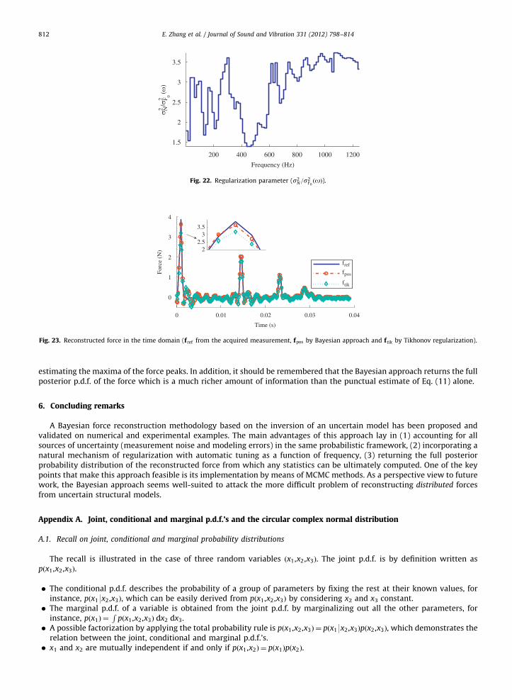
200 400 600 800 1000 1200

1.5

2

2.5

3

3.5

Frequency (Hz)σ2 N

/σ2 F 0 (ω

)

Fig. 22. Regularization parameter (s2N=s2

F0ðoÞ).

0 0.01 0.02 0.03 0.04

0

1

2

3

4

Time (s)

Forc

e (N

) 22.5

33.5

fref

fpos

ftik

Fig. 23. Reconstructed force in the time domain (fref from the acquired measurement, fpos by Bayesian approach and ftik by Tikhonov regularization).

E. Zhang et al. / Journal of Sound and Vibration 331 (2012) 798–814812

estimating the maxima of the force peaks. In addition, it should be remembered that the Bayesian approach returns the fullposterior p.d.f. of the force which is a much richer amount of information than the punctual estimate of Eq. (11) alone.

6. Concluding remarks

A Bayesian force reconstruction methodology based on the inversion of an uncertain model has been proposed andvalidated on numerical and experimental examples. The main advantages of this approach lay in (1) accounting for allsources of uncertainty (measurement noise and modeling errors) in the same probabilistic framework, (2) incorporating anatural mechanism of regularization with automatic tuning as a function of frequency, (3) returning the full posteriorprobability distribution of the reconstructed force from which any statistics can be ultimately computed. One of the keypoints that make this approach feasible is its implementation by means of MCMC methods. As a perspective view to futurework, the Bayesian approach seems well-suited to attack the more difficult problem of reconstructing distributed forcesfrom uncertain structural models.

Appendix A. Joint, conditional and marginal p.d.f.’s and the circular complex normal distribution

A.1. Recall on joint, conditional and marginal probability distributions

The recall is illustrated in the case of three random variables ðx1,x2,x3Þ. The joint p.d.f. is by definition written aspðx1,x2,x3Þ.

�

The conditional p.d.f. describes the probability of a group of parameters by fixing the rest at their known values, forinstance, pðx19x2,x3Þ, which can be easily derived from pðx1,x2,x3Þ by considering x2 and x3 constant. � The marginal p.d.f. of a variable is obtained from the joint p.d.f. by marginalizing out all the other parameters, for

instance, pðx1Þ ¼R

pðx1,x2,x3Þ dx2 dx3.

� A possible factorization by applying the total probability rule is pðx1,x2,x3Þ ¼ pðx19x2,x3Þpðx2,x3Þ, which demonstrates the

relation between the joint, conditional and marginal p.d.f.’s.

� x1 and x2 are mutually independent if and only if pðx1,x2Þ ¼ pðx1Þpðx2Þ.

E. Zhang et al. / Journal of Sound and Vibration 331 (2012) 798–814 813

A.2. Circular complex normal distribution

A complex-value variable x¼ aþ Eb, with independent real-valued real and imaginary parts, a�N ða0,s2x=2Þ and b�N

ðb0,s2x=2Þ, follows a so-called circular complex normal distribution:

pðx9x0,s2x Þ ¼

1

ps2x

expð�ðx�x0Þnðx�x0Þ=s2

x Þ, (A.1)

with x0 ¼ a0þ Eb0.

Appendix B. Detailed description of the conditional p.d.f.’s in Algorithm 1 of Section 3.3

B.1. Conditional p.d.f. of the force

pðF9s�2N ,F0,dC�1

F0c,DÞ ¼ pðF,s�2

N ,F0,dC�1F0c9DÞ=pðs�2

N ,F0,dC�1F0c9I Þ ¼ pð½Y �9F,s�2

N ÞpðF9F0,dC�1F0cÞ: (B.1)

Hence lnðpðF9s�2N ,F0,dC�1

F0c,DÞÞ is written as �nons ln s2

N�Pno

i ¼ 1 ln s2F0ðoiÞ�

Pns

k ¼ 1 ðYk�dHkcFÞnðYk�dHkcFÞ= s2

N�ðF�F0Þn

dC�1F0cðF�F0Þ. Let the derivative qlnðpðF9s�2

N ,F0,dC�1F0c,DÞÞ=qF equal to zero; it returns that the optimal identified force

F ¼ dC FcðPns

k ¼ 1dHkcnYk=s2

NþdC�1F0cF0Þ. Then q2lnðpðF9s�2

N ,F0,dC�1F0c,DÞÞ=qFqFn returns the posterior matrix covariance

dC Fc ¼ ðPns

k ¼ 1dHkcndHkc=s2

NþdC�1F0cÞ�1. As a result, pðF9s�2

N ,F0,dC�1F0c,DÞ ¼N cðF,dC FcÞ.

B.2. Conditional p.d.f. of the variance of measurement and model errors

pðs�2N 9F,DÞ ¼ pð½Y �9F,s�2

N Þpðs�2N 9I Þpðs�2

N ÞðnsnoÞexp �s�2

N

Xns

k ¼ 1

ðYk�dHkcFÞnðYk�dHkcFÞ

!

�ðs�2N ÞðkN�1Þexpð�s�2

N bNÞpGðkN ,bNÞ (B.2)

with kN ¼ ðs�2N ÞðkN þnsnoÞ and bN ¼ ðbNþ

Pns

k ¼ 1ðYk�dHkcFÞnðYk�dHkcFÞÞ.

B.3. Conditional p.d.f. of the prior mean value of the force

pðF0ðlÞ9Fl,s�2F0ðlÞÞppðFl9F0ðlÞ,s�2

F0ðlÞÞpðF0ðlÞ9U0ðlÞ,s2

U0Þpexpð�ðFðlÞ�F0ðlÞIlÞ

nðFðlÞ�F0ðlÞIlÞs�2

F0ðlÞÞ

�expð�ðF0ðlÞ�U0ÞnðF0ðlÞ�U0Þs�2

U0ÞpN cðU0,s�2

U0Þ, (B.3)

where s2U0¼ ð9Dl9s�2

F0ðlÞþs�2

U0Þ�1, U 0 ¼ ðs�2

F0ðlÞ

Pi2Dl

FðoiÞþU0s�2U0Þs2

U0, Il is the column vector of length 9Dl9.

B.4. Conditional p.d.f. of the prior variance of the force

pðs�2F0ðlÞ9FðlÞ,F0ðlÞÞppðFðlÞ9F0ðlÞ,s�2

F0ðlÞÞpðs�2

F0ðlÞ9I Þpðs�2

F0ðlÞÞ9Dl9expð�ðFðlÞ�F0ðlÞIlÞ

nðFðlÞ�F0ðlÞIlÞs�2

F0ðlÞÞ

�ðs�2F0ðlÞÞðkF�1Þexpð�bFs�2

F0ðlÞÞpGðkF ,bF Þ (B.4)

with kF ¼ kFþ9Dl9 and bF ¼ bFþðFðlÞ�F0ðlÞIlÞnðFðlÞ�F0ðlÞIlÞ.

Appendix C. Description of Algorithm 2 of Section 4.2

C.1. Conditional p.d.f. of the coefficients of the force

pðX9D,a,s�2Z ,s2

NÞ ¼

Zpð½Y �9F,a,s�2

N ÞpðF9X,s�2Z Þ dF

� �pðX9I Þp

Zexp �

Xns

k ¼ 1

ðYk�dHkðaÞcFÞnðYk�dHkðaÞcFÞs�2

N

!

�expð�ðF�½B�XÞnðF�½B�XÞs�2Z Þ dFpN cðX,½C X �Þ (C.1)

with ½C X � ¼ ð½B�ndHsðaÞc

nðdHsðaÞcndHsðaÞcs2

Zþs2NÞ�1dHsðaÞc½B�Þ

�1, dHsðaÞc ¼ffiffiffiffiffiffiffiffiffiffiffiffiffiffiffiffiffiffiffiffiffiffiffiffiffiffiffiffiffiffiffiffiffiffiffiffiffiffiffiffiffiffiffiffiffiffiffiffiPns

k ¼ 1dHkðaÞcndHkðaÞc

q, and X ¼ ½C X �½B�

nðdHsðaÞcn

dHsðaÞcs2Zþs2

N�1Pns

k ¼ 1dHkðaÞcnYk.

E. Zhang et al. / Journal of Sound and Vibration 331 (2012) 798–814814

C.2. Sample the modal parameters by Metropolis–Hastings algorithm

At i-th iteration during the MCMC sampling,

�

generate a candidate by drawing a0 � qða9aðiÞÞ � calculate the acceptance probability

gða0,aðiÞÞ ¼minpða09F,s�2

N ,DÞqðaðiÞ9a0ÞpðaðiÞ9F,s�2

N ,DÞqða09aðiÞÞ,1

" #(C.2)

with pða9F,s�2N ,DÞppð½Y �9a,F,s�2

N Þpða9I Þ and qðaÞ a proposal p.d.f., chosen by user.

� Accept or reject by drawing t� Uð0;1Þ, set

aðiþ1Þ ¼a0 if trgða0,aðiÞÞ,aðiÞ otherwise:

((C.3)

References

[1] J. Antoni, J. Daniere, F. Guillet, Effective vibration analysis of ic engines using cyclostationarity. Part I—a methodology for condition monitoring,Journal of Sound and Vibration 257 (2002) 815–837.

[2] J. Mottershead, B. Datta, Special issue on inverse problems in mssp, Mechanical Systems and Signal Processing 23 (2009) 1731–1733.[3] E. Jacquelin, A. Bennani, P. Hamelin, Force reconstruction: analysis and regularization of a deconvolution problem, Journal of Sound and Vibration 265

(2003) 81–107.[4] Q. Lecl�ere, C. Pezerat, B. Laulagnet, L. Polac, Indirect measurement of main bearing loads in an operating diesel engine, Journal of Sound and Vibration

286 (2005) 341–361.[5] Y. Liu, W.S. Shepard Jr., Dynamic force identification based on enhanced least squares and total least-squares schemes in the frequency domain,

Journal of Sound and Vibration 282 (2005) 37–60.[6] H. Choi, A. Thite, D. Thompson, Comparison of methods for parameter selection in Tikhonov regularization with application to inverse force

determination, Journal of Sound and Vibration 304 (2007) 894–917.[7] C. Ma, J. Chang, D. Lin, Input forces estimation of beam structures by an inverse method, Journal of Sound and Vibration 259 (2003) 387–407.[8] F. Gunawan, H. Homma, Y. Kanto, Two-step b-splines regularization method for solving an ill-posed problem of impact-force reconstruction, Journal

of Sound and Vibration 297 (2006) 200–214.[9] S. Granger, L. Perotin, An inverse method for the identification of a distributed random excitation acting on a vibrating structure part 1: theory,

Mechanical Systems and Signal Processing 13 (1999) 53–65.[10] Y. Liu, W.S. Shepard Jr., An improved method for the reconstruction of a distributed force acting on a vibrating structure, Journal of Sound and

Vibration 291 (2006) 369–387.[11] X. Jiang, H. Hu, Reconstruction of distributed dynamic loads on a thin plate via mode-selection and consistent spatial expression, Journal of Sound

and Vibration 323 (2009) 626–644.[12] J. Bendat, A. Piersol, Engineering Applications of Correlation and Spectral, Wiley, 1993.[13] D. Ewins, Modal Testing: Theory, Practice and Application, Wiley, 2001.[14] M. Friswell, J. Mottershead, Finite Element Model Updating in Structural Dynamics, Kluwer Academic Publishers, Dordrecht, 1995.[15] Y. Kim, K. Kim, Indirect input identification by modal filter technique, Mechanical Systems and Signal Processing 13 (1999) 893–910.[16] P. Lee, Bayesian Statistics: An Introduction, Arnold Publication, 1997.[17] A. Tarantola, Inverse Problem Theory and Methods for Model Parameter Estimation, SIAM (Society of Industrial and Applied Mathematics), 2005.[18] J. Rice, Mathematical Statistics and Data Analysis, Duxbury Press, 1995.[19] R. Pintelon, J. Schoukens, System Identification: A Frequency Domain Approach, Wiley, IEEE Press, 2001.[20] A. Tychonoff, V. Arsenin, Solution of Ill-Posed Problems, Winston & Sons, Washington, 1977.[21] W. Hastings, Monte Carlo sampling methods using Markov chains and their applications, Biometrika 57 (1970) 97–109.[22] S. Geman, D. Geman, Stochastic relaxation, Gibbs distributions and the Bayesian restoration of images, IEEE Transactions on Pattern Analysis and

Machine Intelligence 6 (1984) 721–741.[23] W. Gilks, S. Richardson, D. Spiegelhalter, Markov Chain Monte Carlo in Practice, Chapman and Hall, 1995.[24] M. Chen, Q. Shao, J. lbrahim, Monte Carlo Methods in Bayesian Computation, Springer, 2000.[25] K.V. Yuen, Bayesian Methods for Structural Dynamics and Civil Engineering, Wiley, 2010.[26] C. Robert, G. Casella, Monte Carlo Statistical Methods, 2nd ed., Springer, 2004.[27] E. Zhang, Inverse Problem in Structural Dynamics Within Bayesian Framework: Model Updating and Force Reconstruction, PhD Thesis, Universite de

Techonologie de Compi�egne, 2010 (in French).