Bayesian Analysis for Emerging Infectious Diseases

Bayesian Analysis (2009) 4, Number 4, pp. 465–496

Bayesian Analysis for Emerging InfectiousDiseases

Chris P Jewell∗, Theodore Kypraios†, Peter Neal‡ and Gareth O. Roberts§

Abstract. Infectious diseases both within human and animal populations oftenpose serious health and socioeconomic risks. From a statistical perspective, theirprediction is complicated by the fact that no two epidemics are identical due tochanging contact habits, mutations of infectious agents, and changing human andanimal behaviour in response to the presence of an epidemic. Thus model param-eters governing infectious mechanisms will typically be unknown. On the otherhand, epidemic control strategies need to be decided rapidly as data accumulate.In this paper we present a fully Bayesian methodology for performing inferenceand online prediction for epidemics in structured populations. Key features ofour approach are the development of an MCMC- (and adaptive MCMC-) basedmethodology for parameter estimation, epidemic prediction, and online assessmentof risk from currently unobserved infections. We illustrate our methods using twocomplementary studies: an analysis of the 2001 UK Foot and Mouth epidemic,and modelling the potential risk from a possible future Avian Influenza epidemicto the UK Poultry industry.

1 Introduction

Animal disease epidemics in agriculture are potentially devastating in terms of eco-nomics, sociology, and public health. Although there are many diseases that are endemicin UK herds and flocks, there are some from which policy dictates we must remain free(Defra 2007a). These are the so-called notifiable diseases, and are chosen on the basisof their current absence, and risk to the agricultural economy and public health. Thedisadvantage to maintaining a disease-free status is that the population, in the absenceof vaccination, has no prior exposure to the disease and hence a chance to build anacquired immunity. Such populations are therefore highly susceptible to the accidentalintroduction of disease which, if the transmission mechanisms allow, will run uncheckedon a national scale.

Responding to such accidental outbreaks is a problem faced by governmental au-thorities, and the design of national-scale disease control measures prior to an outbreakis a high priority. Nevertheless, since epidemic outbreaks are rare and tend to be-have differently to one-another, a high degree of flexibility must be maintained withincontrol-policies to adapt to unexpected features of an epidemic in progress.

∗Department of Mathematics and Statistics, Lancaster University, UK, mailto:chris.jewell@

warwick.ac.uk†School of Mathematical Sciences, University of Nottingham, UK, mailto:theodore.kypraios@

nottingham.ac.uk‡School of Mathematics, University of Manchester, UK, mailto:[email protected]§Department of Statistics, University of Warwick, UK, mailto:[email protected]

c© 2009 International Society for Bayesian Analysis DOI:10.1214/09-BA417

mailto:[email protected]






466 Bayesian Analysis for Emerging Infectious Diseases

This paper presents a unified Bayesian approach that can be used to inform policyadaptation during disease outbreaks. First we develop a generic modelling frameworkat the population level. Here, individual elements of the ‘population’ can be chosenaccording to the specific application at hand (eg individual animal, barn, farm, etc.).Our methodology is illustrated by two extended case studies of recent popular interest:the 2001 UK Foot-and-Mouth epidemic (FMD), and the prospect of a future HighlyPathogenic Avian Influenza epidemic (HPAI) within the UK poultry industry. In bothcases, the population consists of UK farms of the relevant type. Before describing themotivating examples in detail, we give a brief background to parametric inference forinfectious disease spread along with motivation for the key aspects of the methodologyto be used in the analysis.

Excellent reviews of classical approaches to analyzing epidemic data, such as mar-tingale methods and generalized linear models are given in Becker (1989) and Beckerand Britton (1999). However, statistical inference for infectious disease models hastaken off with the introduction of MCMC Gibson (1997); Gibson and Renshaw (1998);O’Neill and Roberts (1999). This is primarily because infectious disease data usuallysuffers from the complaint that the data which is available is incomplete, making theevaluation of the model likelihood difficult. Therefore, data augmentation (imputation)forms a key aspect of any MCMC algorithm to analyze such data. Data augmen-tation is usually a very straightforward procedure. However, there is often a strongdependence between the model parameters and the imputed data which can lead toslow convergence of the MCMC algorithm. Non-centered reparameterizations (see, Pa-paspiliopoulos et al. (2003)) have been developed to improve the convergence rates ofMCMC algorithms where there is a strong dependence between the model parametersand the imputed data. This approach has been successfully applied to epidemic modelsin Neal and Roberts (2005) and Kypraios (2007) and we give an outline and refinementof the methodology in Section 2.5.

As with many statistical models, neither the full posterior distribution of the modelparameters nor the conditional posterior distributions of the model parameters followstandard probability distributions. Therefore a Gibbs sampler algorithm is inappropri-ate and a random walk Metropolis (rwM) algorithm is a natural candidate. Supposethat there are p model parameters and that θ (a p-dimensional vector) is the cur-rent value of the model parameters based upon the MCMC algorithm. Then in the(Gaussian) rwM algorithm we propose new values θ′ for the model parameters from amultivariate Gaussian distribution with mean θ and covariance matrix Σ. The choiceof Σ is crucial to the efficiency of the MCMC algorithm. Often if p is small, Σ is finetuned through pilot runs of the algorithm. However this takes time and if p ≥ 10 thiscan become infeasible in conjunction with real-time analysis of data. Real-time dataanalysis is crucially important in seeking to control emerging diseases. A solution isoffered by adaptive MCMC (see, Haario et al. (2001), Roberts and Rosenthal (2007))which updates Σ based upon the performance of the algorithm. This produces an ef-ficient MCMC algorithm which automatically tunes itself, thus making the algorithmapplicable for analysing data in real-time. This is further assisted by the parallelizationof the computer code. Parallel computing is a computational rather than statistical

C. P. Jewell, T. Kypraios, P. Neal and G. O. Roberts 467

issue, but does have a large bearing on the size of data sets which can be analyzed in areasonable time frame. Therefore this is an important issue for MCMC practitioners tobe aware of, even if it is not always an issue.

The paper is structured as follows. In section 3 the motivating examples Foot-and-Mouth disease and Avian influenza are introduced in detail. However, first in section 2we introduce the methodology. Whilst the methodology is described with the motivatingexamples in mind, it is sufficiently general to be applied to a whole host of agriculturalepidemics. The results of the analysis FMD and HPAI are given in section 3 withconcluding discussion in section 4.

2 Generic Methodology

Before we describe our specific implementations for FMD and HPAI, we will discussa generic methodology applicable to all disease epidemics. We therefore begin by de-scribing the epidemic model, followed by the construction of a likelihood expression forthe model parameters. Having derived the likelihood, we consider the practical prob-lems that arise from the fact that our observation of the epidemic process is necessarilyincomplete. Throughout we highlight the novel aspects of the model and their analysis.

2.1 Introduction

The main motivation for the research was the risk analysis of emerging infectious dis-eases through UK farms. Therefore the key aspect of the analysis is obtaining anunderstanding of the transmission mechanism between individual farms. As a result wemodel the disease on the macroscopic farm level rather than the microscopic individuallevel. The epidemic model is defined as follows:

Consider a total population of size N farms. We assume that at any given timepoint each farm i can be in one of four states:

• Susceptible premises (S) do not have the disease and are able to be infected by it.

• Infected premises (I) have the disease and are able to infect susceptible premises.Their infectivity increases as a function of time.

• Notified premises (N) have been detected as having the disease and are subjectto government-imposed movement restrictions. However, they are still capable ofinfecting susceptibles by other means, such that their infectivity is curbed at alower level.

• Removed premises (R), in the case of both FMD and HPAI, have had their animalsculled and therefore play no further part in the epidemic.

The only transitions in state we allow are: from susceptible to infected, from infectedto notified, and from notified to removed. There are two features which we shall impose


on the model which are worthy of extra comment at this stage. Firstly, we allow theinfection rate of a farm to vary with time. This corresponds to the within-farm epidemicleading to the infection of more and more individual animals over time. We are implicitlyassuming that, within the interval between a farm’s infection and notification, that thefarm is infectious the infectivity is increasing and not significantly affected by the deathor recovery of animals. For FMD and HPAI this assumption is reasonable. Often whenmodeling the disease at an animal level the infection period is divided into a latent period(ie infected but not yet infectious) followed by an infectious period with a constantrate of infectivity. However, the time varying infectivity is more natural/biologicallyplausible at the macroscopic level than assuming a step function for the infectivity offarms (latent/infectious period). Secondly, it is assumed that a farm is infected onlyonce from outside sources. This implies that we treat the herd or flock of animals presenton a farm as a single entity. This is a reasonable assumption when the intra-herd/flockinfection rate dominates the inter-farm infection rate which is the case for FMD andHPAI.

We assume that the epidemic is observed up to a certain time, say Tobs. Denote bynI , nN and nR, the total number of premises who got infected, notified and removedby time Tobs, respectively. The exact relationship between nI , nN and nR will dependupon the culling regime imposed. Finally, note that we assume that only notified farmsare removed (culled). The methodology can easily be adapted to other cases such asthe culling of contiguous premises.

2.2 Infectious Process

We assume that an infectious farm i makes infectious contacts with a given farm j atthe points of a time inhomogeneous Poisson point process with transmission rate attime t:

βij(t) = Tijh(t− Ii), (1)

where Ii denotes the point of time at which farm i becomes infected, Tij is a measureof the association/infectivity between farms i and j and h(·) represents how a farm’sinfectivity changes over time. In particular, we choose

0 < h(s) ≤ 1 s > 0h(s) = 0 s ≤ 0.

The function h(·) is problem-specific and the choice of this function is discussed later.In particular in Section 3, h(s) = 1 (s > 0), a step function, and h(s) = eνs/(µ + eνs)(s > 0) are used for FMD and HPAI, respectively.

Let It, Nt and St denote the sets of infected, notified and susceptible farms, at time


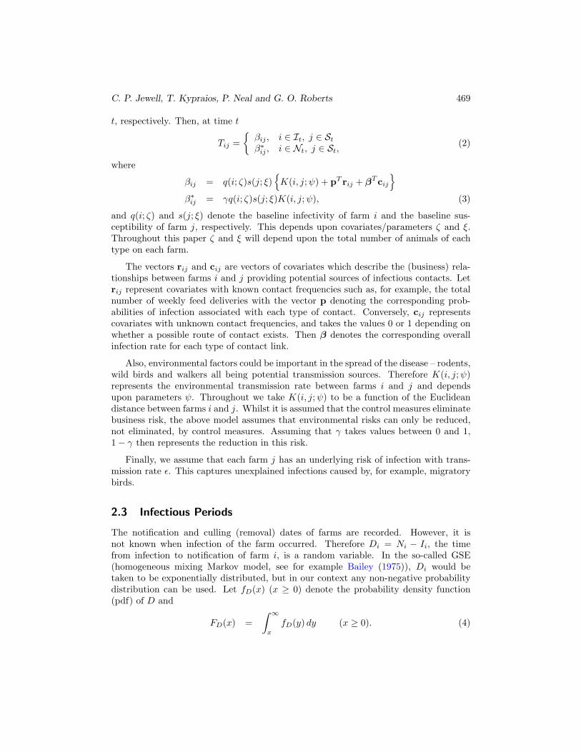
t, respectively. Then, at time t

Tij =

βij , i ∈ It, j ∈ St

β∗ij , i ∈ Nt, j ∈ St,(2)

where

βij = q(i; ζ)s(j; ξ)

K(i, j; ψ) + pT rij + βT cij

β∗ij = γq(i; ζ)s(j; ξ)K(i, j; ψ), (3)

and q(i; ζ) and s(j; ξ) denote the baseline infectivity of farm i and the baseline sus-ceptibility of farm j, respectively. This depends upon covariates/parameters ζ and ξ.Throughout this paper ζ and ξ will depend upon the total number of animals of eachtype on each farm.

The vectors rij and cij are vectors of covariates which describe the (business) rela-tionships between farms i and j providing potential sources of infectious contacts. Letrij represent covariates with known contact frequencies such as, for example, the totalnumber of weekly feed deliveries with the vector p denoting the corresponding prob-abilities of infection associated with each type of contact. Conversely, cij representscovariates with unknown contact frequencies, and takes the values 0 or 1 depending onwhether a possible route of contact exists. Then β denotes the corresponding overallinfection rate for each type of contact link.

Also, environmental factors could be important in the spread of the disease – rodents,wild birds and walkers all being potential transmission sources. Therefore K(i, j;ψ)represents the environmental transmission rate between farms i and j and dependsupon parameters ψ. Throughout we take K(i, j; ψ) to be a function of the Euclideandistance between farms i and j. Whilst it is assumed that the control measures eliminatebusiness risk, the above model assumes that environmental risks can only be reduced,not eliminated, by control measures. Assuming that γ takes values between 0 and 1,1− γ then represents the reduction in this risk.

Finally, we assume that each farm j has an underlying risk of infection with trans-mission rate ε. This captures unexplained infections caused by, for example, migratorybirds.

2.3 Infectious Periods

The notification and culling (removal) dates of farms are recorded. However, it isnot known when infection of the farm occurred. Therefore Di = Ni − Ii, the timefrom infection to notification of farm i, is a random variable. In the so-called GSE(homogeneous mixing Markov model, see for example Bailey (1975)), Di would betaken to be exponentially distributed, but in our context any non-negative probabilitydistribution can be used. Let fD(x) (x ≥ 0) denote the probability density function(pdf) of D and

FD(x) =∫ ∞

x

fD(y) dy (x ≥ 0). (4)


The choice of D will be problem specific.

2.4 Likelihood

Having described the epidemic process, we turn to the question of statistical inference.Let I, N and R denote the infection, notification and removal times, respectively. Notethat up to time Tobs, N and R are known, whilst both the total number nI and thetimes of I of infections are unknown. Let θ = (ψ, β, γ, ε, ζ, ξ) and α denote the infectionand infectious period (i.e. D – time from infection to notification) parameters, respec-tively. The likelihood of the data (the epidemic outbreak) given the model parameterscan then be expressed as the product of the infection terms and the infectious periodterms. Before giving the likelihood, however, we introduce some notation. We label thepremises that become infected up to time Tobs by i = 1, 2, . . . , nI and the remainder byi = nI +1, nI +2, . . . , N . We adopt the notation that if premise j is never infected thenIj = Nj = Rj = ∞. A premises j just prior to becoming infected receives infectiouspressure from the premises in the sets Yj− and Y∗

j−.

Yj− := i : Ii < Ij ≤ NiY∗

j− := i : Ni < Ij ≤ RiThus the likelihood is given by

L(I,N,R|θ, α) ∝nI∏

j 6=κ

ε +

∑

i∈Yj−

βij(Ij) +∑

i∈Y∗j−

β∗ij(Ij)

× exp

−

∫ Tobs

Iκ

(∑i∈St

ε +∑i∈It

∑j∈St

βij(t− Ii) +∑i∈Nt

∑j∈St

β∗ij(t− Ii)

)dt

×nI∏i=1

fD(Ni − Ii), (5)

where κ denotes the label of the initial infective farm with Iκ its corresponding infectiontime. The parameter ε represents the (additive) unexplained background infectiouspressure. The term in the exponent is termed the total infectious pressure and we shalldenote this by S.

In our examples, we shall use independent Gamma priors for each of the parameters,i.e. parameter µ has prior f(µ) ∼ Ga(λµ, νµ). Thus

f(θ,α|I,N,R) ∝ L(I,N,R|θ, α)×∏

µ∈θ,α

f(µ). (6)

For the infection parameters θ, none of the parameters have standard conditional distri-butions. Our approach uses a simple random walk Metropolis (within Gibbs) algorithm.The infectious period parameters will be studied in detail shortly.

The first step before we give the MCMC algorithm is to simplify (5). In particular, wecan rewrite, S, the integral on line two of (5) as a double sum which is both illuminating


and easy to calculate. For t ≥ 0, let H(t) =∫ t

0h(s) ds. Then since βij(t) = βijh(t),

S =∫ Tobs

Iκ

∑

i∈St

ε +∑

i∈It

∑

j∈St

βij(t− Ii) +∑

i∈Nt

∑

j∈St

β?ij(t− Ii)

dt

= ε

N∑

i=1

Tobs ∧ Ii − Iκ+nI∑

i=1

N∑

j=1

H(Tobs ∧Ni ∧ Ij − Ii ∧ Ij)βij

+nN∑

i=1

N∑

j=1

H(Tobs ∧Ri ∧ Ij − Ii ∧ Ij)−H(Tobs ∧Ni ∧ Ij − Ii ∧ Ij)β?ij

(7)

2.5 Non-centering

For missing data problems, MCMC convergence is often significantly improved by theadoption of a non-centered parameterization (see Papaspiliopoulos et al. (2003) for areview). Such parameterizations orthogonalize prior structure, and work particularlywell when components of the missing data are poorly identified by observations.

Since I is unknown and can be treated as a parameter in the model, a standard(centered) Metropolis-within-Gibbs MCMC procedure would carry out the followingsteps.

1. For each i, update θi|α, θi−, I,N,R.

2. For each i, update αi|θ,αi−, I,N,R.

3. For each i, update Ii|θ, α, Ii−,N,R.

A non-centered construction for our epidemic model with missing infection timescan be constructed as follows. We focus on non-centering of the infectious period Di =Ni−Ii. Subscripts will be omitted for clarity, but it is understood that this constructioncan be carried out for some or all infection events.

We introduce U , apriori independent of α, such that DD= φ(U ; α). Thus, for

1 ≤ i ≤ nI , we can reparameterise the model in terms of U rather than I with

Ii = Ni −Di = Ni − φ(Ui, α) (8)

For this parameterization, updating α conditional on U simultaneously results in up-dating I. I is also updated by changing U = (U1, U2, . . . , UnI

) for fixed α.

It turns out to be important to use a compromise between centering and non-centering, resulting in so-called partial non-centered methods (see Papaspiliopoulos et al.(2003); Neal and Roberts (2005); Kypraios (2007)). There are a number of ways of con-structing these methods. The approach we adopt here chooses, at each iteration at


random, a collection of infectious periods to be centered, and others non-centered. Letµ denote the probability that an infectious period is non-centered. For 1 ≤ i ≤ nI , let

Zi =

1 with probability µ,0 with probability 1− µ.

(9)

Set A = i : Zi = 1 (non-centered individuals) and B = i : Zi = 0 (centeredindividuals) with for i ∈ A, Ii = φ(Ui, α). We have the following partially non-centeredMCMC algorithm:

1. Update Z and hence, A and B using (9).

2. For each i, update θi|θi−, α,UA, IB,N,R.

3. For each i, update αi(IA)|αi−,θ,UA, IB,N,R.

4. For each i, update Ii = φ(Ui,α)|θ, α, Ii−,N,R.

2.6 Unknown number of infections

The above approach is applicable if nI is known and all the notification times are known.For example, analysing a past epidemic such as the 2001 FMD outbreak. However, ifthe epidemic is in progress, all that is known is that nI = nN +m where nN denotes thetotal number of notified premises and 0 ≤ m ≤ N − nN . Therefore we include nI as aparameter in the model and have to incorporate MCMC moves for the addition/deletionof infection times. We call premises which are infected but not notified by time Tobs,occult premises. The MCMC algorithm is therefore modified to the following:

1. For each i, update θi|α, θi−, I,N,R.

2. For each i, update αi|θ,αi−, I,N,R.

3. For each i, update Ii|θ, α, Ii−,N,R.

4. Propose an occult infection: I → I + o5. Propose to delete an occult infection: I → I − o

Note the above algorithm is based upon an extension of the centered algorithm butcould just as easily be added to the partial non-centered algorithm described in section2.5. The last two steps involve changing the dimension of I, with a correspondingchange of dimension of S, such that whenever we add an infection, [I] increases by one,and [S] decreases by one. The reverse is true for deletion, while for moving an infectiontime, both [I] and [S] remain constant. These, therefore, constitute reversible jumpmoves the proposal of which is implementation-specific. This will be discussed furtherin section 3.2, where, since the infectious period distribution is assumed to be known,a partially non-centered algorithm is not applicable.


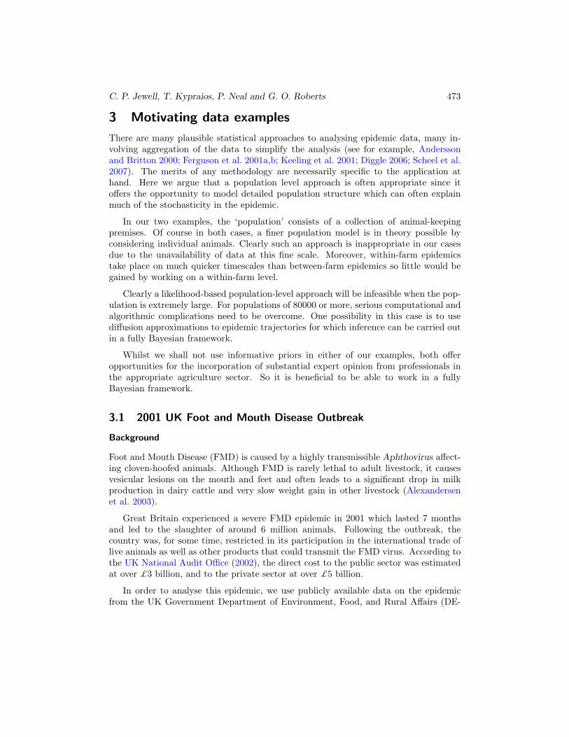
3 Motivating data examples

There are many plausible statistical approaches to analysing epidemic data, many in-volving aggregation of the data to simplify the analysis (see for example, Anderssonand Britton 2000; Ferguson et al. 2001a,b; Keeling et al. 2001; Diggle 2006; Scheel et al.2007). The merits of any methodology are necessarily specific to the application athand. Here we argue that a population level approach is often appropriate since itoffers the opportunity to model detailed population structure which can often explainmuch of the stochasticity in the epidemic.

In our two examples, the ‘population’ consists of a collection of animal-keepingpremises. Of course in both cases, a finer population model is in theory possible byconsidering individual animals. Clearly such an approach is inappropriate in our casesdue to the unavailability of data at this fine scale. Moreover, within-farm epidemicstake place on much quicker timescales than between-farm epidemics so little would begained by working on a within-farm level.

Clearly a likelihood-based population-level approach will be infeasible when the pop-ulation is extremely large. For populations of 80000 or more, serious computational andalgorithmic complications need to be overcome. One possibility in this case is to usediffusion approximations to epidemic trajectories for which inference can be carried outin a fully Bayesian framework.

Whilst we shall not use informative priors in either of our examples, both offeropportunities for the incorporation of substantial expert opinion from professionals inthe appropriate agriculture sector. So it is beneficial to be able to work in a fullyBayesian framework.

3.1 2001 UK Foot and Mouth Disease Outbreak

Background

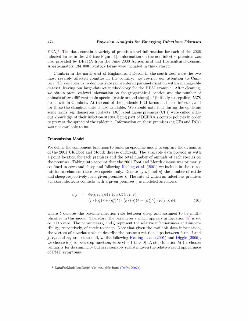
Foot and Mouth Disease (FMD) is caused by a highly transmissible Aphthovirus affect-ing cloven-hoofed animals. Although FMD is rarely lethal to adult livestock, it causesvesicular lesions on the mouth and feet and often leads to a significant drop in milkproduction in dairy cattle and very slow weight gain in other livestock (Alexandersenet al. 2003).

Great Britain experienced a severe FMD epidemic in 2001 which lasted 7 monthsand led to the slaughter of around 6 million animals. Following the outbreak, thecountry was, for some time, restricted in its participation in the international trade oflive animals as well as other products that could transmit the FMD virus. According tothe UK National Audit Office (2002), the direct cost to the public sector was estimatedat over £3 billion, and to the private sector at over £5 billion.

In order to analyse this epidemic, we use publicly available data on the epidemicfrom the UK Government Department of Environment, Food, and Rural Affairs (DE-


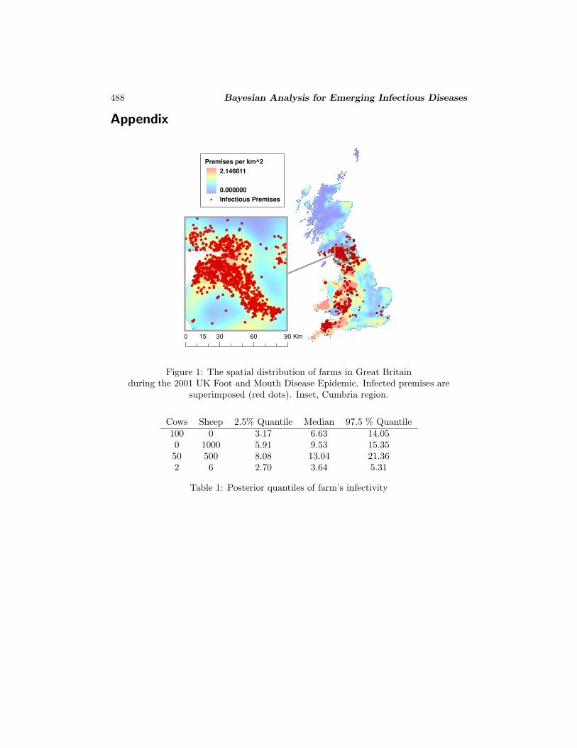
FRA)1. The data contain a variety of premises-level information for each of the 2026infected farms in the UK (see Figure 1). Information on the non-infected premises wasalso provided by DEFRA from the June 2000 Agricultural and Horticultural Census.Approximately 134, 000 livestock farms were included in this dataset.

Cumbria in the north-west of England and Devon in the south-west were the twomost severely affected counties in the country: we restrict our attention to Cum-bria. This enables us to demonstrate non-centered parameterization with a manageabledataset, leaving our large-dataset methodology for the HPAI example. After cleaning,we obtain premises-level information on the geographical location and the number ofanimals of two different main species (cattle or/and sheep) of (initially susceptible) 5378farms within Cumbria. At the end of the epidemic 1021 farms had been infected, andfor these the slaughter date is also available. We should note that during the epidemicsome farms (eg. dangerous contacts (DC), contiguous premises (CP)) were culled with-out knowledge of their infection status, being part of DEFRA’s control policies in orderto prevent the spread of the epidemic. Information on these premises (eg CPs and DCs)was not available to us.

Transmission Model

We define the component functions to build an epidemic model to capture the dynamicsof the 2001 UK Foot and Mouth disease outbreak. The available data provide us witha point location for each premises and the total number of animals of each species onthe premises. Taking into account that the 2001 Foot and Mouth disease was primarilyconfined to cows and sheep and following Keeling et al. (2001) we include in the trans-mission mechanism these two species only. Denote by nc

i and nsi the number of cattle

and sheep respectively for a given premises i. The rate at which an infectious premisesi makes infectious contacts with a given premises j is modeled as follows:

βij = δq(i; ζ, χ)s(j; ξ, χ)K(i, j; ψ)= (ζ · (nc

i )χ + (ns

i )χ) · (ξ · (nc

j)χ + (ns

j)χ) ·K(i, j;ψ), (10)

where δ denotes the baseline infection rate between sheep and assumed to be multi-plicative in this model. Therefore, the parameter ε which appears in Equation (5) is setequal to zero. The parameters ζ and ξ represent the relative infectiousness and suscep-tibility, respectively, of cattle to sheep. Note that given the available data information,the vectors of covariates which describe the business relationships between farms i andj, rij and cij are set to null, whilst following Keeling et al. (2001) and Diggle (2006),we choose h(·) to be a step-function, ie. h(s) = 1 (s > 0). A step-function h(·) is chosenprimarily for its simplicity but is reasonably realistic given the relative rapid appearanceof FMD symptoms.

1‘DataForModellersOct03.xls, available from (Defra 2007a)


Specific modeling details

An important issue regarding the transmission kernel is whether or not the Euclideanmetric is the most appropriate distance measure, especially when an outbreak takes placein a geographical area with rich landscape such as hills, mountains and lakes. Regardingthe FMD outbreak in the UK, Savill et al. (2006) showed that the Euclidean distancemetric between infectious and susceptible premises is a better predictor of transmissionrisk than the shortest and quickest routes via road, except where major geographicalfeatures intervene. Therefore, they concluded that a simple spatial transmission kernelbased on Euclidean distance suffices in most regions, probably reflecting the multiplicityof potential transmission routes during the epidemic.

Therefore, due to the lack of geographical information on the landscape of Cumbria,the difficulty of obtaining metrics such as minimum walking distances and taking intoaccount the results presented in Savill et al. (2006) we adopt the Euclidean metric. Forreasons of robustness, it is prudent to adopt a heavy-tailed transmission kernel. There-fore if ρ(i, j) denote the Euclidean distance between farms i and j, the environmentalspread is modeled by taking a Cauchy-type kernel

K(ρi,j , ψ) =ψ

ρ2ij + ψ2

.

We adopt a simpler version of the full SINR model assuming that each farm i atany given time point can be either susceptible, infected or removed. Thus the modelcan be seen as a heterogeneously mixing stochastic SIR model. In order to illustratethe performance of the non-centering methodology in such a context, we assume thatD ∼ Ga(a, b) with a = 4, fixed, and b an unknown parameter to be estimated. Notethat this leads to a bell-shaped distribution where the mean (or the mode) and thevariance depends only on b, see Kypraios (2007) for more details. Whilst, the choice ofa = 4 is somewhat arbitrary, it is supported by the model fit analysis performed, seesection 3.1 below.

MCMC Algorithm

We wish to make inference for (θ, b) where θ = (δ, ζ, ξ, χ, ψ), so we are assuming that theinfection times of each of the infected premises are considered to be unknown. FollowingSubsection 2.5 we adopt a partially non-centered approach. We reparameterise Di asDi

D= b · Ui where U ∼ Ga(a, 1) with U and b a priori independent. Furthermore, sincewe are making inference on b, we use a Gamma prior. We therefore implement thefollowing MCMC algorithm:

1. Choose i uniformly at random and update Ii|Ii−, b, θ, R.

2. Update b|I,θ,R.

3. Update Z and hence, A and B using (9).


4. Update b|θ,UA, IB,R using the partially non-centered algorithm.(Note that for i ∈ A, Ii is also updated).

5. Update θ|b, I,R.

Note that the above algorithm is the partially non-centered algorithm of section 2.5with the inclusion of a draw of b from its conditional distribution,

π (b|I,R, a) ∼ Ga

(anI + λb,

nI∑

i=1

(Ri − Ii) + νb

), (11)

step 2. Step 2 is included because it improves the mixing of the MCMC algorithm forminimal computational cost. We chose to non-center 25% of the infection times (i.e.µ = 0.25) at each iteration as this was found to produce an efficient algorithm (step3) according to a pilot study which was carried out to seek for the “optimal” choiceof µ. Step 4 is performed using a Metropolis-Hastings algorithm with b proposed from(11). Finally, step 1 is repeated a number of times in each iteration to improve themixing of the algorithm. The model parameters θ are updated in block, step 5, using amultiplicative random walk Metropolis algorithm.

An Illustrative Example

The following example is taken from Kypraios (2007) and the interested reader is re-ferred there for more details. A dataset has been simulated consisting of N = 500initially susceptibles and one initially infective individual uniformly located in a square[0, 1]× [0, 1]. A distance-dependent infection rate and a Gamma infectious period withknown shape parameter have been considered. Assuming that we only observed theremoval times of each individual, a centered and a partially non-centered algorithm(similar to the one described in the previous section 3.1) were implemented such thatto obtain samples from the posterior distribution of the scale parameter of the Gammadistribution. Figure 2 shows that the non-centered algorithm performs significantlybetter than the centered algorithm.

Results

In this section we present a Bayesian analysis of the 2001 FMD outbreak in Cumbriaby using the model described in section 3.1, using a partially non-centered approach asexplained in 3.1. Non-informative priors were chosen for all the parameters.

In Figure 3, we present the posterior distribution of b, the scale parameter for theinfectious period distribution. Directly as a result of this we give the posterior meaninfectious period. It agrees with the assumptions made in Keeling et al. (2001), althoughin Keeling et al. (2001) they considered an SEIR-type model where the exposed andthe infectious periods are assumed to be known and fixed without any variability ordifferences between premises.


Figure 4 depicts the posterior distribution of the spatial transmission kernel. Pos-terior uncertainty is illustrated through the superposition of kernels drawn from theposterior. The kernel is shown on a log scale (see Figure 5) and the modal value agreeswell with other literature (see for example, Keeling et al. 2001). An interesting featureof the kernel is the fact that there appears to be little infectious pressure exerted overa distance of more than about 4km, a result which is also in association with otherpublished work (see for example, Keeling et al. 2001; Deardon et al. 2007; Diggle 2006).

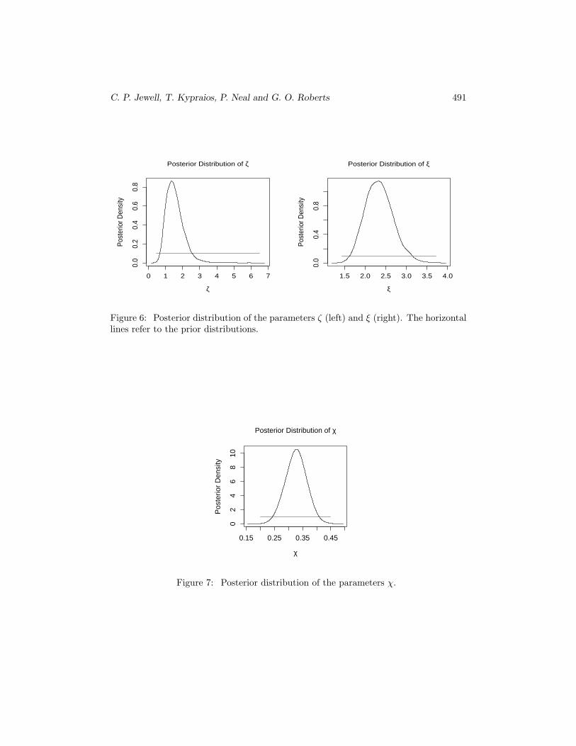
Having obtained the marginal distributions of the relative infectiousness and suscep-tibility of cattle to sheep (see Figures 6) we can infer that each individual cow was morelikely to transmit the disease and also likely to be more susceptible to the disease thaneach individual sheep. Moreover, there is strong evidence for a non-linear effect of thenumber of different species in each farm (see Figure 7). These results are qualitativelysimilar to those reported in Keeling et al. (2001), Diggle (2006) and Deardon et al.(2007) although the former only looks at the case where χ = 1.

For illustrative purposes we turn our attention to the infectivity q(i; ζ, χ) and thesusceptibility s(i; ξ, χ) for farms of typical size. An average medium-size farm which hasonly cattle, an average medium-size farm which has only sheep as well as an averagelarge- and small-size farm with cattle and sheep have been considered (see Table 1 andTable 4). An interesting result from these tables is that a typical medium-size sheepfarm is more infectious than a typical medium-size farm with cattle (only). In addition,a medium-size cattle and a medium-size sheep farm are both similarly susceptible toinfection. Furthermore, both tables reveal that there is a significant risk to susceptiblefarms from small holdings with a handful of animals. Therefore, we can conclude thatall animal holdings, however small, play an important role in the spread of the disease.

Model fit

It is important to assess the appropriateness of the model proposed to the epidemic data.For practical purposes, measures of model fit based on predictive accuracy are importantin particular applications. Implementation of these measures are easily applied and arewidely used for epidemics (see for example Lekone and Finkenstadt (2006); Cauchemezand Ferguson (2008)).

Instead, we focus on using non-centered residuals to assess model fit (Papaspiliopou-los 2003). The suitability of the infectious period distribution is straightforward andquick to check by examining the distribution of the non-centred variables Ui. If themodel fits well, then the population of Ui’s ranging over premises and MCMC iterationsshould be approximately Gamma(4, 1) distributed, as specified in Section 3.1. Figure8 shows a good agreement between these two distributions. In addition, to check ourassumption of a fixed a = 4, we ran the algorithm with a as an unknown parameter.The posterior mode of a was 3.76, with the fixed value well within the support.


3.2 High Pathogenicity Avian Influenza

Background

In 1996, High Pathogenicity Avian Influenza H5N1 (HPAI) emerged as a disease of geesein southern China and began to spread throughout south-east Asia (Xu et al. 1999; Claaset al. 1998). In 2005, outbreaks were recorded in eastern Europe with multiple cases inwild birds and a large outbreak in domestic poultry in Romania. Sporadic cases havesince appeared further west in France, Denmark, Germany, Sweden, and more recentlythe UK (European Centre for Disease Surveillance 2006).

The poultry industry is a large economic force in the UK, with 1.5 million tonnes ofmeat produced in 2004 representing 40% of the primary meat market. The possibility ofan HPAI epidemic therefore poses a significant economic risk (Defra 2007b). In addition,it has been shown that a significant human health risk exists in that people with highexposure to the virus have been infected with high mortality (Claas et al. 1998; WHO2007). Therefore the implications of an outbreak of HPAI are very serious, and hence,its classification as a notifiable disease which means that any outbreak in the UK mustbe eliminated.

For the Poultry Industry, covariate data was obtained from DEFRA in the form ofthe Great Britain Poultry Register (GBPR) and Poultry Network Data (PND). Aftercleaning, these data give premises-level information on the geographical location, pro-duction type, and commercial contacts of 8636 poultry premises within Great Britain. Inour analysis only production-level premises are included since the breeding sector oper-ates extremely high biosecurity and is considered to present negligible risk in the event ofan outbreak. This assumption is further strengthened by the industry supposition thatall live-bird movement (apart from transport to slaughterhouses) would immediatelycease in the event of an unfolding epidemic2. Furthermore, since the production-levelrelies on a low-frequency “all-in-all-out” system with birds arriving from the breed-ing sector and going directly to the slaughterhouse upon departure, market-mediatedtransmission as seen for FMD in the cattle, sheep, and pig industries is not considered.

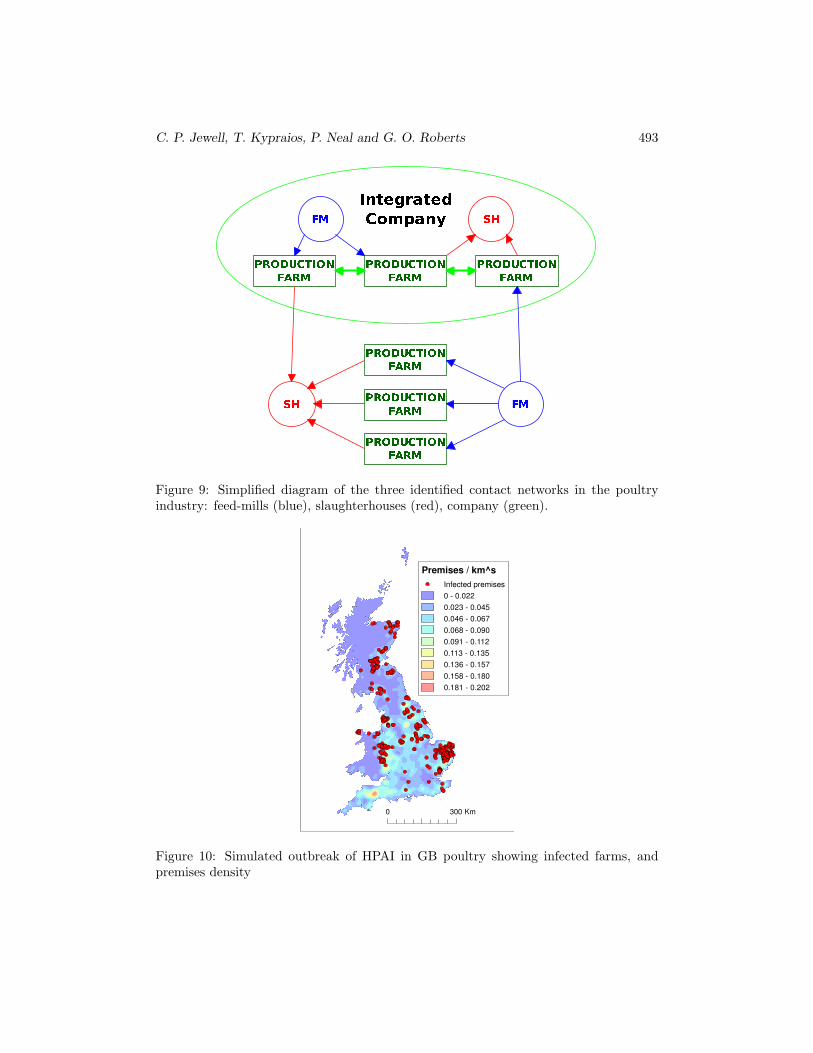
In comparison to the livestock industry, the UK poultry industry is highly structured.Besides spatial proximity, potential infectious contact within the industry is governed byproduction type and managemental networks. Firstly, the GBPR currently characterizes11 production types (Table 3) all of which are relatively isolated from each other, andmay have differential susceptibilities to disease. Secondly, large integrated productioncompanies, representing about 60% of the broiler premises, have only limited contactwith the independent producers that make up the remainder of the industry. Premisesbelonging to the same company may, due to the sharing of equipment and personnel,transmit disease between themselves, but be relatively isolated from other companiesand the independent sector. We have also identified that transmission of disease mayoccur via third-party feed-mills and slaughterhouses (Figure 9). From the PND, it ispossible to estimate the frequencies of feed mill and slaughterhouse contacts, and ofthe number of farms each feed mill or slaughterhouse services. Finally, there is the

2Confirmed at a meeting with poultry industry representatives, 01/03/2007


possibility of disease transmission by other networks such as egg collection and catchingteams (employed to “thin” populations of housed birds prior to final depopulation).However, scant data is available for such networks and consultation with the poultryindustry indicates that these networks operate on a local scale and may, therefore, bemodeled spatially. Since there has been no major outbreak of HPAI in the UK thusfar, a simulated outbreak in the Great Britain poultry industry (Figure 10) is usedto show how our statistical methodology can be applied to perform inference on suchan epidemic in real-time, and stochastic simulation used over the results to provide aquantitative risk analysis.

Transmission model

We now define our component functions to provide an inference mechanism for HPAI.The covariate data give information about production type (spt(j)), distance betweenpremises (ρ(i, j)), the company affiliation (if any) (CCP ), and the rate of lorry contactsfor feed mill (RFM ) and slaughterhouse (RSH) networks. For the poultry industry, itis not clear how flock size might affect either premises level infectivity or susceptibility.Without any further information, it would be impossible to identify infectivity fromsusceptibility; we therefore use only production-type susceptibility on the susceptiblepremises, spt(j). This represents categorical data and is therefore modeled as a multi-plicative factor with 11 levels according to the production types in the dataset (Table3). We choose susceptibility to be a property of the major production-type on eachpremises j relative to broilers, such that for broilers the corresponding parameter is setto 1. Thus we attempt to identify industry sectors that might be at higher risk duringan outbreak. For this data, in contrast to FMD, we use the full SINR model to give:

βij = spt(j)(p1r

FMij + p2r

SHij + β1c

CPij + β2e

−δρ(i,j))

(12)

and

β?ij = spt(j)

(γβ2e

−δρ(i,j))

. (13)

The distance kernel, K(i, j;ψ) is taken to be exponential in this case. We thereforeperform inference on θ = spt, p1, p2, β1, β2, γ, δ, where spt is the vector of production-type susceptibilities.

Infectious Period

For the infectious period, we use a Gumbel distribution with pdf

fD(x) = abebx−a(ebx−1) (14)

andFD(x) = e−a(ebx−1). (15)


This allows flexibility of modeling, and interpretations of a and b as the rate ofdetection, and rate of development of clinical signs throughout the flock, respectively.These parameters are estimated from literature and expert opinion and consequentlyfor the analysis a and b are assumed to be known, fixed constants.

The farm-level infectivity function, h (·), is specified as:

h(s) =eνs

µ + eνs, (16)

satisfying the conditions in Section 2.2 and which is easily integrated to

H(t) =∫ t

0

h(s)ds =1ν

log(

µ + eνt

µ + 1

). (17)

MCMC Algorithm

For HPAI, we require an MCMC algorithm that is not only robust to the problem, butthat is also fast enough to support the real-time aspect of the inference. We use theMCMC algorithm specified in section 2.6 with certain implementation-specific modifi-cations. Step 1 uses a multisite update of θ. We use multiplicative random walk forthis 95% of the time, and additive random walk 5% of the time to allow components ofθ to “escape” from small values. Step 2 is omitted since we are not making inferenceon the parameters of the infectious period distribution. However, the remaining stepsare worthy of further explanation.

Firstly, steps 3, 4 and 5 are not executed sequentially in a deterministic fashion.Rather, we choose each step with equal probability a number of times per iteration ofthe MCMC. In the following descriptions, we denote a move by I − t + s, an additionby I + s, and a deletion by I − t.

Step 3 Move an infection time: We choose an infection time to move from a discreteuniform distribution, U[1, [I]], and propose a replacement infection time drawnfrom the distribution D defined either in (14) if the notification time is known, orin (19) if not. We accept the proposed value with probability

1 ∧ L(I − t+ s|N ,R, θ)L(I|N , R,θ)

×Q,

where

Q =

fD(Nt−It)fD(Nt−Is) infection known

FD(Tobs−It)FD(Tobs−Is) infection occult.


Step 4 Add an infection: We choose an occult infection from the susceptibles using adiscrete uniform distribution U[1, [S]]. An infection time is then drawn from thedistribution in Equation 19. We accept such an addition with probability:

1 ∧ L(I + s|N ,R, θ)L(I|N ,R, θ)

× [S](m + 1) · g(Tobs − Is)

,

where m is the number of previously added infections prior to the addition andTobs − Is is sampled from a non-negative pdf g(·). The choice of g(·) is discussedbelow.

Step 5 Delete an infection. We choose an infection time to delete from a discreteuniform distribution over the premises that have been previously added. Weaccept such a move with probability:

1 ∧ L(I − t|N ,R,θ)L(I|N , R, θ)

× m · g(Tobs − It)[S] + 1

where m is the number of previously added infections prior to the deletion.

In order to efficiently propose occult infection times for the MCMC, we would liketo sample from:

g(x) ∝ FD(x) (x ≥ 0) (18)

Due to the specification of (15) it is non-trivial to simulate directly from a distribu-tion with pdf proportional to FD(·). For algorithmic speed we prefer to avoid rejectionsampling in favor of a truncated Normal approximation, obtained by a 2nd order TaylorSeries expansion of (15), giving:

T − Ii ∼ N(−1

b,

1ab2

), T − Ii ≥ 0 (19)

Simulation studies showed that such an independence sampler achieves an acceptanceprobability greater than 0.5.

Adaptive MCMC

One of the barriers to implementing such an algorithm for real-time inference is the timeneeded to tune random-walk proposal densities. Multisite updating of the transmissionparameters (β) was chosen to minimise the time-consuming need of fully recalculatingthe likelihood, but manually adjusting the order-16 proposal variance-covariance ma-trix would, conversely, be a very long process. To relieve this issue, we use the adaptiveproposal scheme of Haario et al. (2001). This is implemented following work by Roberts


and Rosenthal (2007), and Andrieu and Moulines (2006) on theory to guarantee ergod-icity of the resulting Markov chain, and allows the proposal density to adapt for optimalscaling as the chain converges. The proposal density, therefore, is:

Qn(x, ·) = (1− ξ)N(x, (2.38)2Σd/d) + ξN(x, (0.1)2Id/d), (20)

where Σd is the d-dimensional empirical variance-covariance matrix of the current pos-terior density with d = 16 and ξ is a small positive constant which following Robertsand Rosenthal (2007) we take ξ = 0.05.

Parallel Computing

Finally, to speed up the calculation of the likelihood, domain-decomposition paral-lelization of the sums in (7) was achieved using a shared-memory architecture with animplementation of the OpenMP standard (Dagum and Menon 1998). This was chosenover a distributed architecture since the dependent nature of the epidemic data requireshigh levels of inter-process communication; the high-bandwidth busses on a multipro-cessor mainboard being many times faster than network interconnects. We were ableto achieve a 10-fold speedup in algorithm runtime on a 8 dual-core Sun X4600 serverrunning Linux, giving a final runtime of 4.5 hours for 100000 iterations with this dataset.

Results

In order to demonstrate our methods, we use a simulated Avian Influenza epidemic inthe UK poultry industry. We start by using a stochastic simulation on the dataset of8636 premises, creating an epidemic that lasts for 77 days and infects a total of 375premises. We then choose to observe this epidemic at three time points: 14, 25, and50 days after the first notification (Table 4, Figure 10). At each observation time, weuse the data available to perform risk-prediction, and show how this is refined as theepidemic progresses.

We begin with posterior parameter distributions, and Figure 11 plots the prior andposteriors for β2 at three observation times. This illustrates how posterior uncertaintyand prior dependence recedes during the course of the epidemic.

We also consider the Bayes predictive probability (risk) that a given farm becomesinfected during the current epidemic. This is estimated by off-line forward model sim-ulation under parameter values drawn randomly from the posterior distribution of theparameters at the current time. This is an example of a dynamic quantity which variesas the epidemic evolves (as well as due to the changing parameter posterior distribu-tions). These are shown pictorially in Figure 12, and demonstrate how the risk estimateprogresses with time and amount of information available.

For control purposes, it may be of interest to know which premises would presenta high risk to the remaining susceptibles if they themselves were to be infected. Wedefine Ri to be the expected number of further premises a premises, i, would infect were


it to be the index infection in a hypothetical infection where all other farms started assusceptibles, and conditional on all parameters. Ri plays the role of a farm-specificbasic reproduction number. For each premises we calculate the posterior probability:P (Ri > 1).

However P (Ri > 1) does not discriminate between farms which infect “large Ri

farms” and those which do not. Thus within our very heterogenous population, P (Ri >1) does not necessarily indicate the degree of risk posed by a premises to the population.Instead, we prefer to take a bootstrap expectation of the epidemic size that would resultif each premises were to be the index case for the epidemic. To illustrate this, we havetaken two premises from our dataset with differing P (Ri > 1), and have run stochasticsimulations over the joint posterior for the transmission and removal rates (Table 5).

In terms of active disease control surveillance, a more efficient policy might be totarget limited resources to suspect premises. Of primary concern is the number of oc-cult infections present at any one time as a measure of how much control effort will beneeded when these infections are detected. The reversible jump algorithm allows us toassign a probability of being infected to each apparently susceptible premises at eachobservation time, thus identifying high-occult probability locations. The probabilitiescan then be plotted in a similar fashion to Figure 12 (results not shown) or monitoredin an appropriate way. Of statistical interest are the posteriors of the number of occultsat each time point (Figure 13). Early in the epidemic, the algorithm overestimates thenumber of occults, consistent with the high degree of uncertainty in the parameter pos-teriors, and the influence of conservatively chosen priors. However, this effect disappearslater in the epidemic.

4 Discussion

In this paper particular attention has been paid to the generality of the modellingframework, the computational and algorithmic efficiency of the MCMC algorithms par-ticularly for incomplete epidemics where risk assessment crucially depends upon thepossible presence of occult infections. We also allow for two different types of network:those which describe a non-specific connectivity (such as company contacts), and thosewhich explicitly describe risk caused by particular activities (eg feed lorry deliveries,slaughter house visits, etc.). However, there are many important issues we have notconsidered in any detail.

We have not focused here on the evaluation of control strategies, although ourmethodology provides a natural framework for doing this for specific applications. Fromour on-line simulation study, two important issues emerge. Control strategies are mostinfluential very early in the course of an epidemic. It is therefore important to be ableto subsume all available expert information into prior distributions for parameters atthe outset, so as to be well-informed about parameters early on to guide the evolution ofcontrol policy. Secondly, data from the early stages of an epidemic are often augmentedby contact tracing information which can often identify disease transmission pathways,and hence add substantially to the available information on model parameters gov-


erning the transmission of infections. We are currently extending our methodology toincorporate this information into our likelihood-based framework.

More fundamentally is the issue of network data quality, particularly with respectto contact rate information. In our HPAI example, we use network data that is derivedfrom a questionnaire sample of approximately 30% of the premises registered in theGBPR. From this, we have simulated contact rates on the feed mill and slaughter housenetworks for the remaining 70% of premises. This will inevitably lead to inaccuraciesin our predictions when working at the individual level. An important extension of ourmethodology will, therefore, be to allow for uncertainty in the network specification andtherefore reflect this in the prediction.

We have shown in our FMD example that use of non-centred variables for assessmentof model fit is a convenient method for outbreak data. Building on this, model choicefor epidemic models in a fully Bayesian framework could be easily performed usingstandard methodology (eg reversible jump MCMC or marginal likelihood), and part ofour ongoing work is to address this.

In summary, we have introduced a unified modelling inference and prediction method-ology for emerging infectious disease epidemics within a Bayesian framework. We haveapplied this to two important agricultural contexts, demonstrating complementary sit-uations in which our approach can be applied. It is therefore anticipated that ourmethodology could be used for informing control strategy in future epidemics in a widerange of populations.

ReferencesAlexandersen, S., Zhang, Z., Donaldson, A. I., and Garland, A. J. M. (2003). “The

pathogenesis and diagnosis of foot-and-mouth disease.” J. Comp. Pathol., 129(1):1–36. 473

Andersson, H. and Britton, T. (2000). Stochastic epidemic models and their statisticalanalysis, volume 151 of Lecture Notes in Statistics. New York: Springer-Verlag. 473

Andrieu, C. and Moulines, E. (2006). “On the ergodicity properties of some adaptiveMCMC algorithms.” Annals of Applied Probability , 16: 1462–1505. 482

Bailey, N. T. J. (1975). The mathematical theory of infectious diseases and its appli-cations. Hafner Press [Macmillan Publishing Co., Inc.] New York, second edition.469

Becker, N. G. (1989). Analysis of infectious disease data. Monographs on Statistics andApplied Probability. London: Chapman & Hall. 466

Becker, N. G. and Britton, T. (1999). “Statistical studies of infectious disease incidence.”J. R. Stat. Soc. Ser. B Stat. Methodol., 61(2): 287–307. 466


Cauchemez, S. and Ferguson, N. (2008). “Likelihood-based estimation of continuous-time epidemic models from time-series data: application to measles transmission inLondon.” J. R. Soc. Interface, 5: 885–897. 477

Claas, E., Osterhaus, A., van Beek, R., De Jong, J., Rimmelzwaan, G., Senne, D.,Krauss, S., Shortridge, K., and Webster, R. (1998). “Human influenza A (H5N1)virus related to a highly pathogenic avian influenza virus.” The Lancet, 351: 472.478

Dagum, L. and Menon, R. (1998). “OpenMP: an Industry Standard API for Shared-memory Programming.” IEEE Comput. Sci. Eng., 5: 46–55. 482

Deardon, R., Brooks, S. P., Grenfell, B., Keeling, M. J., Tildesley, M. J. S. S. J.,Shaw, D., and Woolhouse, M. E. J. (2007). “Inference for individual-level models ofinfectious diseases in large populations.” Submitted. 477

Defra (2007a). “Defra Website.” [Online; Accessed 24-04-2007].URL http://www.defra.gov.uk 465, 474

— (2007b). “Eggs and poultry facts and statistics.” [Online; Accessed 12-01-2007].URL http://www.defra.gov.uk/foodrin/poultry/statistics/index.htm 478

Diggle, P. J. (2006). “Spatio-temporal point processes, partial likelihood, foot andmouth disease.” Stat. Methods Med. Res., 15(4): 325–336. 473, 474, 477

European Centre for Disease Surveillance (2006). “Weekly surveillance report.” EuroSurveill., 11(51): pii=3098.URL http://www.eurosurveillance.org/ViewArticle.aspx?ArticleId=3098478

Ferguson, N. M., Donnelly, C. A., and Anderson, R. M. (2001a). “The Foot-and-MouthEpidemic in Great Britain: Pattern of Spread and Impact of Interventions.” Science,292(5519): 1155–1161. 473

— (2001b). “Transmission intensity and impact of control policies on the foot andmouth epidemic in Great Britain.” Nature, 413: 542–547. 473

Gibson, G. (1997). “Markov chain Monte Carlo methods for ftting spatiotemporalstochastic models in plant epidemiology.” Applied Statistics, 46(2): 215–233. 466

Gibson, G. and Renshaw, E. (1998). “Estimating parameters in stochastic compart-mental models using Markov Chain methods.” IMA J. Math. Appl. Med. Biol., 15:19–40. 466

Haario, H., Saksman, E., and Tamminen, J. (2001). “An adaptive metropolis algo-rithm.” Bernoulli, 7(2): 223–242. 466, 481

Keeling, M. J., Woolhouse, M. E. J., Shaw, D. J., Matthews, L., Chase-Topping, M.,Haydon, D. T., Cornell, S. J., Kappey, J., Wilesmith, J., and Grenfell, B. T. (2001).“Dynamics of the 2001 UK Foot and Mouth Epidemic: Stochastic Dispersal in aHeterogeneous Landscape.” Science, 294(5543): 813–818. 473, 474, 476, 477

http://www.defra.gov.uk

http://www.defra.gov.uk/foodrin/poultry/statistics/index.htm

http://www.eurosurveillance.org/ViewArticle.aspx?ArticleId=3098


Kypraios, T. (2007). “Efficient Bayesian Inference for Partially Observed StochasticEpidemics and A New class of Semi−Parametric Time Series Models.” Ph.D. thesis,Department of Mathematics and Statistics, Lancaster University, Lancaster. Avail-able from http://www.maths.nott.ac.uk/personal/tk/files/Kyp07.pdf. 466,471, 475, 476

Lekone, P. and Finkenstadt, B. (2006). “Statistical Inference in a Stochastic EpidemicSEIR Model with Control Intervention: Ebola as a Case Study.” Biometrics, 62:1170–1177. 477

Neal, P. and Roberts, G. (2005). “A case study in non-centering for data augmentation:stochastic epidemics.” Stat. Comput., 15(4): 315–327. 466, 471

O’Neill, P. D. and Roberts, G. O. (1999). “Bayesian inference for partially observedstochastic epidemics.” J. Roy. Statist. Soc. Ser. A, 162: 121–129. 466

Papaspiliopoulos, O. (2003). “Non-centered parametrisations for hierarchical modelsand data augmentation.” Ph.D. thesis, Department of Mathematics and Statistics,Lancaster University, Lancaster. 477

Papaspiliopoulos, O., Roberts, G. O., and Skold, M. (2003). “Non-centered parame-terizations for hierarchical models and data augmentation.” In Bayesian statistics, 7(Tenerife, 2002), 307–326. New York: Oxford Univ. Press. Editors J. M. Bernardoand M. J. Bayarri and J. O. Berger and A. P. Dawid and D. Heckerman and A. F.M. Smith and M. West. 466, 471

Roberts, G. and Rosenthal, J. (2007). “Coupling and Ergodicity of adaptive Markovchain Monte Carlo algorithms.” Journal of Applied Probability , 44: 458–475. 466,481, 482

Savill, N. J., Shaw, D. J., Deardon, R., Tildesley, M. J., Keeling, M. J., Woolhouse,M. E., Brooks, S. P., and Grenfell, B. T. (2006). “Topographic determinants offoot and mouth disease transmission in the UK 2001 epidemic.” BMC Vet Res, 2.Available at doi:10.1186/1746-6148-2-3. 475

Scheel, I., Aldrin, M., Frigessi, A., and Jansen, P. A. (2007). “A stochastic model forinfectious salmon anemia (ISA) in Atlantic salmon farming.” J. R. Soc. Interface, 4:699–706. 473

UK National Audit Office (2002). “The 2001 outbreak of foot and mouth disease.”Report by the Comptroller and auditor general, HC 939, Session 2001-2002, London:The Stationery Office. 473

WHO (2007). “Avian Influenza.” [Online; Accessed 12-01-2007].URL http://www.who.int/csr/disease/avian_influenza/en/index.html 478

Xu, X., Subbarao, K., Cox, N., and Guot, Y. (1999). “Genetic Characterization ofthe Pathogenic Influenza A/Goose/Guangdond/1/96 (H5N1) Virus: Similarity of ItsHemagglutinin Gene to Those of H5N1 Viruses fromthe 1997 Outbreaks in HongKong.” Virology , 261: 15. 478

http://www.who.int/csr/disease/avian_influenza/en/index.html


Acknowledgments

Thanks to Dr RM Christley and Dr SE Robinson, Department of Clinical Studies, Faculty of

Veterinary Science, University of Liverpool; Streamline Computing Ltd for the loan of the Sun

X4600 server, and Dr Mike Pacey for his help and advice with it; Dr Miles Thomas, DEFRA

Central Scientific Laboratory, for providing the Foot-and-Mouth data; DEFRA for providing

covariate information on the GB Poultry Industry.


Appendix

Premises per km^2

2.146611

0.000000

Infectious Premises

0 30 60 9015 Km

Figure 1: The spatial distribution of farms in Great Britainduring the 2001 UK Foot and Mouth Disease Epidemic. Infected premises are

superimposed (red dots). Inset, Cumbria region.

Cows Sheep 2.5% Quantile Median 97.5 % Quantile100 0 3.17 6.63 14.050 1000 5.91 9.53 15.3550 500 8.08 13.04 21.362 6 2.70 3.64 5.31

Table 1: Posterior quantiles of farm’s infectivity


0 500 1000

0.0

0.2

0.4

0.6

0.8

1.0

Lag

ACF

Centered

0 500 1000

0.0

0.2

0.4

0.6

0.8

1.0

Lag

ACF

Partially Non Centered

Figure 2: Comparison of ACFs of the scale parameter between the standard (centered)and the non-centered algorithm for simulated example.

0.40 0.50 0.60

05

1015

Posterior Distribution of b

b

Pos

terio

r D

ensi

ty

6.0 6.5 7.0 7.5 8.0 8.5 9.0 9.5

0.0

0.2

0.4

0.6

0.8

1.0

Posterior Distribution of the Mean Infectious Period

days

Pos

terio

r D

ensi

ty

Figure 3: Posterior distribution of the parameter b (left) and the average infectiousperiod of a single farm 4.0/b (right). The red/horizontal line indicates the prior chosenfor b.

Cows Sheep 2.5% Quantile Median 97.5 % Quantile100 0 6.10 10.43 17.580 1000 5.91 9.53 15.3550 500 10.21 15.93 24.752 6 3.76 4.70 5.94

Table 2: Posterior quantiles of farm’s susceptibility


0 2 4 6 8 10

0.0

0.4

0.8

Spatial Kernel

distance (in Km)

K(i,

j, ψ)

0.005 0.007 0.009

020

040

060

0

Posterior Distribution of ψ

ψP

oste

rior

Den

sity

Figure 4: The marginal posterior distribution of ψ (right) and a 95% HPDR of K(i, j;ψ)(left). The black/solid line of the latter refers to the modal shape of the kernel basedon the posterior mode of parameter ψ.

−2 −1 0 1 2

−5

−3

−1

0

Spatial Kernel (log scale)

log(distance) in Km

log(

K(i,

j), ψ)

Figure 5: The spatial kernel K(i, j; ψ) on log-scale drawn by using the modal value ofthe posterior distribution of ψ.


0 1 2 3 4 5 6 7

0.0

0.2

0.4

0.6

0.8

Posterior Distribution of ζ

ζ

Pos

terio

r Den

sity

1.5 2.0 2.5 3.0 3.5 4.0

0.0

0.4

0.8

Posterior Distribution of ξ

ξ

Pos

terio

r Den

sity

Figure 6: Posterior distribution of the parameters ζ (left) and ξ (right). The horizontallines refer to the prior distributions.

0.15 0.25 0.35 0.45

02

46

810

Posterior Distribution of χ

χ

Pos

terio

r D

ensi

ty

Figure 7: Posterior distribution of the parameters χ.


Histograms of the `Residuals’

Den

sity

0 5 10 15 20

0.00

0.05

0.10

0.15

0.20

0.25

Figure 8: Posterior distribution of non-centered variables Ui for the FMD example.The red/solid line, showing a Gamma(4, 1), indicates good model fit.

Production Type Number of premises % total datasetBroilers 1416 16.4

Chicken Layers 3733 43.2Turkey 668 7.7

Duck Meat 239 2.8Duck Layers 85 1.0Goose Meat 57 0.7Goose Layers 17 0.2

Pheasant 2011 23.3Partridge 376 4.4

Quail Layers 34 0.4Total 8636 100

Table 3: Production-type distribution within the dataset.

Time / days # notified infections occult infections

14 10 1525 61 1350 290 40

Table 4: The state of the epidemic at each observation time

P(Ri > 1) Ei,β,γ [epidemic size]0.01 30.95 184

Table 5: Expected epidemic size starting at premises with different Ris.


Figure 9: Simplified diagram of the three identified contact networks in the poultryindustry: feed-mills (blue), slaughterhouses (red), company (green).

0 300 Km

Premises / km^s

Infected premises

0 - 0.022

0.023 - 0.045

0.046 - 0.067

0.068 - 0.090

0.091 - 0.112

0.113 - 0.135

0.136 - 0.157

0.158 - 0.180

0.181 - 0.202

Figure 10: Simulated outbreak of HPAI in GB poultry showing infected farms, andpremises density


Figure 11: The prior and posteriors for β2 at the three time points during the epidemic


Day 14 Day 25

Day 50

Infection Risk

0.401 - 1.000

0.201 - 0.400

0.101 - 0.200

0.051 - 0.100

0.000 - 0.050

Figure 12: Spatial distribution of predicted risk to the population


(a) Day 14

(b) Day 25

(c) Day 50

Figure 13: Posterior distributions of the number of occult infections. The red/verticalline denotes the true number, determined from the simulated data ( T=10:, T=25:,T=50).

Bayesian Analysis for Emerging Infectious Diseases

Documents

Transcript of Bayesian Analysis for Emerging Infectious Diseases