Battery Life Verification Test Manual
133
INEEL/EXT-04-01986 Ad v anced Technolo g y Dev elopmen t Pro g ram For Lithium-Ion Batteries Battery Technolo gy L ife Verif ication Test Manual February 2005 Idaho National Laboratory Idaho Falls, ID 83415 Operated by Battelle Energy Alliance, LLC FreedomCAR & Vehicle Technologi es Program
Transcript of Battery Life Verification Test Manual

8/11/2019 Battery Life Verification Test Manual
http://slidepdf.com/reader/full/battery-life-verification-test-manual 1/133
INEEL/EXT-04-01986
Advanced Technology Development ProgramFor Lithium-Ion Batteries
Battery Technology Life Verif icationTest Manual
February 2005
Idaho National LaboratoryIdaho Falls, ID 83415Operated by Battelle Energy Alliance, LLC
FreedomCAR & Vehicle
Technologies Program

8/11/2019 Battery Life Verification Test Manual
http://slidepdf.com/reader/full/battery-life-verification-test-manual 2/133
Disclaimer
This report was prepared as an account of work sponsored by an agency of the United StatesGovernment. Neither the United States Government nor any agency thereof, nor any of their employees, makesany warranty, express or implied, or assumes any legal liability or responsibility for the accuracy, completeness,or usefulness of any information, apparatus, product, or process disclosed, or represents that its use would notinfringe privately owned rights. References herein to any specific commercial product, process, or service bytrade name, trademark, manufacturer, or otherwise does not necessarily constitute or imply its endorsement,recommendation, or favoring by the United States Government or any agency thereof. The views and opinionsof authors expressed herein do not necessarily state or reflect those of the United States Government or anyagency thereof.

8/11/2019 Battery Life Verification Test Manual
http://slidepdf.com/reader/full/battery-life-verification-test-manual 3/133

8/11/2019 Battery Life Verification Test Manual
http://slidepdf.com/reader/full/battery-life-verification-test-manual 4/133
ii

8/11/2019 Battery Life Verification Test Manual
http://slidepdf.com/reader/full/battery-life-verification-test-manual 5/133
iii
CONTENTS
GLOSSARY OF LIFE TESTING TERMS ................................................................................................ vii
ACRONYMS............................................................................................................................................... ix
1. INTRODUCTION.............................................................................................................................. 1
1.1 FreedomCAR Battery Life Goals.......................................................................................... 1
1.2 Battery Technology Life Verification Objectives ................................................................. 1
1.3 Battery Life Test Matrix Design Approach...........................................................................2
1.4 Reference Performance Testing Approach............................................................................ 3
1.5 Life Test Data Analysis Approach ........................................................................................ 3
1.6 Organization of the Manual................................................................................................... 3
2. LIFE TEST EXPERIMENT DESIGN REQUIREMENTS ............................................................... 5
2.1 Technology Characterization Requirements ......................................................................... 5
2.2 Core Life Test Matrix Design Requirements ........................................................................ 9
2.3 Core Life Test Matrix Design and Verification...................................................................12
2.3.1 Preliminary Design Stage.................................................................................. 132.3.2 Final Design Stage ............................................................................................172.3.3 Final Verification Stage ....................................................................................18
2.4 Supplemental Life Test Matrix Design Requirements ........................................................19
2.4.1 Experimental Plan to Assess Path Independence.............................................. 202.4.2 Experimental Plan to Assess Cold-Start Operation...........................................202.4.3 Experimental Plan to Assess Low-Temperature Operation .............................. 21
3. LIFE TEST PROCEDURES ............................................................................................................22
3.1 Initial Characterization Tests............................................................................................... 22
3.1.1 General Test Conditions and Scaling ................................................................ 233.1.2 Minimum Characterization for All Cells...........................................................243.1.3 Additional Characterization of Selected Cells ..................................................24
3.1.4 BOL Reference Testing..................................................................................... 263.2 Core Life Test Matrix.......................................................................................................... 26
3.2.1 Stand Life (Calendar Life) Testing ................................................................... 263.2.2 Cycle Life (Operating) Testing ......................................................................... 273.2.3 Reference Performance Tests and End-of-Test Criteria....................................28
3.3 Supplemental Life Tests ...................................................................................................... 29
3.3.1 Combined Calendar and Cycle Life Tests......................................................... 29

8/11/2019 Battery Life Verification Test Manual
http://slidepdf.com/reader/full/battery-life-verification-test-manual 6/133
iv
3.3.2 Cold-cranking Power Verification Tests...........................................................303.3.3 Low-temperature Operation Tests.....................................................................30
4. DATA ANALYSIS AND REPORTING......................................................................................... 32
4.1 Initial Performance Characterization Test Results .............................................................. 32
4.1.1 Determination of Open Circuit Voltage versus State of Charge .......................334.1.2 Capacity Verification ........................................................................................334.1.3 Determine Temperature Coefficient of ASI (Selected Cells)............................ 334.1.4 Pulse Power Verification (MPPC) ....................................................................344.1.5 Pulse Power Verification (HPPC) ..................................................................... 344.1.6 Rank Ordering of Cells ..................................................................................... 354.1.7 Self-Discharge Rate Characterization ............................................................... 364.1.8 Cold-Cranking Power Verification ................................................................... 364.1.9 AC EIS Characterization................................................................................... 364.1.10 ASI Noise Characterization............................................................................... 36
4.2 Core Matrix Life Test Results ............................................................................................. 39
4.2.1 Life on Test Estimates....................................................................................... 394.2.2 Calendar Life Estimate......................................................................................414.2.3 Effects of Cycling Stresses................................................................................ 434.2.4 Life in Service Estimate ....................................................................................44
4.3 Supplemental Life Test Results........................................................................................... 45
4.3.1 Hypothesis Testing............................................................................................454.3.2 Combined Calendar/Cycle Life tests................................................................. 454.3.3 Cold-start Verification Tests ............................................................................. 474.3.4 Low-temperature Operation Tests.....................................................................48
5. REFERENCES................................................................................................................................. 49
Appendix A—Life Test Simulation Program ........................................................................................... A-1
Appendix B—Methods for Modeling Life Test Data ............................................................................... B-1
Appendix C—Study of Life-Limiting Mechanisms in High-Power Li-Ion Cells .................................... C-1
Appendix D—Use of the Monte Carlo Simulation Tool ..........................................................................D-1
Appendix E—Test Measurement Requirements....................................................................................... E-1
FIGURES
Figure 2.1-1. Example of ASI "truth" functions. ......................................................................................... 8
Figure 2.3-1. Results for life test matrix example (estimated (±1 std dev) versus true life on test). ......... 18
Figure 4.2-1. Comparison of bootstrap results with normal distribution for life on test at Calendar Life 1test condition. ................................................................................................................................... 41
Figure 4.3-1. Expected ASI histories for combined cycle/calendar and calendar/cycle test conditions.... 46
8/11/2019 Battery Life Verification Test Manual
http://slidepdf.com/reader/full/battery-life-verification-test-manual 7/133
v
TABLES
2.1-1. Test conditions for the minimum life test experiment example. ....................................................... 6
2.1-2. Hypothetical results from short-term tests of new and aged cells. .................................................... 7
2.1-3. Estimated acceleration factors for the Minimum Life Test Experiment Example. ........................... 8
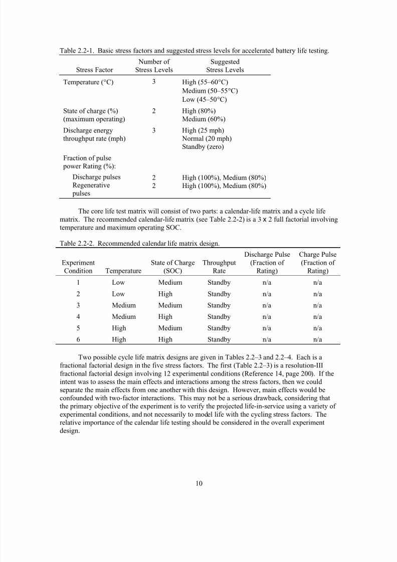
2.2-1. Basic stress factors and suggested stress levels for accelerated battery life testing. ....................... 10
2.2-2. Recommended calendar life matrix design...................................................................................... 10
2.2-3. Cycle life matrix design (Design 1)................................................................................................. 11
2.2-4. Cycle life matrix design (Design 2)................................................................................................. 11
2.3-1. Expected lives on test for the Minimum Life Test Experiment example. ....................................... 14
2.3-2. Preliminary allocation of cells for the Minimum Life Test Experiment example........................... 16
2.3-3. Simulation results for the Minimum Life Test Experiment example. ............................................. 17
3.2-1. Reference performance test intervals for life testing. ...................................................................... 29
4.2-1. Simulated experimental results: estimates compared with truth...................................................... 40
4.2-2. Data and results for calendar life estimation for example matrix. ................................................... 43
4.2-3. Data and results for estimation of cycle life acceleration factors for example matrix..................... 44

8/11/2019 Battery Life Verification Test Manual
http://slidepdf.com/reader/full/battery-life-verification-test-manual 8/133

8/11/2019 Battery Life Verification Test Manual
http://slidepdf.com/reader/full/battery-life-verification-test-manual 9/133
vii
GLOSSARY OF LIFE TESTING TERMS
Acceleration Factor – Ratio of calendar life to life on test.
Area-Specific Impedance (ASI) – The impedance of a device relative to the electrode area of thedevice, defined as the change in cell voltage (V) as a result of a change in cell currentdivided by the change in cell current (A), all multiplied by the active superficial cell area(cm2), ohm-cm2.
Available Capacity – The capacity (in Ah) of a device between two state of charge conditionsdesignated as SOCMAX and SOCMIN, as measured using a C1/1 constant current dischargerate after the performance of a HPPC pulse profile at SOCMAX,
Beginning of Life (BOL) – The point in time at which life testing begins. A distinction is made inthis manual between the performance of a battery at this point and its initial performance, because some degradation may take place during early testing before the start of lifetesting. Analysis of the effects of life testing is based on changes from the BOL performance.
C-rate – A current (for discharge or charge) expressed as a multiple of the rated device capacity(in ampere-hours) for a reference (static capacity) discharge. For example, for a devicehaving a capacity of 1 ampere-hour under this reference condition, a 5-A rate would be5A/(1 Ah) or 5C, hr -1.
C 1 /1 Rate – The rate corresponding to completely discharging a fully charged device in exactlyone hour. Otherwise, a rate corresponding to the manufacturer’s rated capacity (inampere-hours) for a one-hour constant current discharge. For example, if the battery’srated one-hour capacity is 1 Ah, then the C1/1 constant current rate is 1 A. The C1/1 rateis the reference discharge rate for power-assist applications; other applications may havedifferent reference rates, hr -1.
Calendar Life (LCAL) – The time required to reach end of life at the reference temperature of 30ºCat open-circuit (corresponding to key-off/standby conditions in the vehicle).
Depth of Discharge – The percentage of a device’s rated capacity removed by discharge relativeto a fully charged condition, normally referenced to a constant current discharge at theC1/1 rate. The capacity to be used is established (fixed) at the beginning of testing, %.
End of Life (EOL) – A condition reached when the device under test is no longer capable of meeting the applicable FreedomCAR goals. This is normally determined from RPTresults, and it may not coincide exactly with the ability to perform the life test profile(especially if cycling is done at elevated temperatures.) The number of test profiles
executed at end of test is not necessarily equal to the cycle life per the FreedomCAR goals.
End of Test (EOT) – The point in time where life testing is halted, either because criteriaspecified in the test plan are reached, or because it is not possible to continue testing.
Hybrid Pulse Power Characterization (HPPC) – A test whose results are used to calculate pulse power and energy capability under FreedomCAR operating conditions.

8/11/2019 Battery Life Verification Test Manual
http://slidepdf.com/reader/full/battery-life-verification-test-manual 10/133
viii
Life in service – The time required to reach end of life at the nominal conditions of normal usagein the vehicle (30ºC and specified cycling conditions).
Life on test (LTEST ) – The time required to reach end of life at the test conditions specified for accelerated life testing.
Minimum Pulse Power Characterization (MPPC) – A shortened version of the Hybrid PulsePower Characterization test conducted periodically to measure performance deteriorationover time.
SOC MAX and SOC MIN – Two state of charge conditions that are chosen as reference conditions for a given life test program. They could represent the entire anticipated operating range for a given application, although for reference test purposes they are typically limited to therange of SOC values used in the life test matrix. SOCMAX and SOCMIN are represented by(i.e., measured as) the corresponding open circuit voltages when the device is in a stablecondition (see Stable SOC Condition and Stable Voltage Condition.) SOCMAX can beselected as any value less than or equal to the maximum allowable operating voltage for adevice. SOCMIN can be any value less than SOCMAX and greater than or equal to the
minimum allowable operating voltage, %.
Stable SOC (state of charge) Condition – For a device at thermal equilibrium, its state of chargeunder clamped voltage conditions is considered to have reached a stable value when thecurrent declines to less than 1% of its original or limiting value, averaged over at least5 minutes. (For example, if a device is discharged at a C1/1 rate and then clamped at afinal voltage, the SOC would be considered stable when the current declines to 0.01 C1/1or less.)
Stable Voltage Condition – For a device at thermal equilibrium, its open circuit voltage (OCV) isconsidered stable if it is changing at a rate of less than 1% per hour when measured over at least 30 minutes. (Note that a stable voltage condition can also be reached by setting
an arbitrary OCV rest interval (e.g., 1 hour), which is long enough to ensure that voltageequilibrium is reached at any SOC and temperature condition of interest. This is muchsimpler to implement with most battery testers than a rate-of-change criterion. However,it would result in a longer test and in longer rest intervals, which could be undesirable if adevice had high self-discharge at the temperature where the test was conducted.)
State of Charge (SOC ) – The available capacity in a battery expressed as a percentage of actualcapacity. This is normally referenced to a constant current discharge at the C1/1 rate. For this manual, it may also be determined by a voltage obtained from a correlation of capacity to voltage fixed at beginning of life. SOC = (100 – DOD) if the rated capacity isequal to the actual capacity, %.
State-of-health (SOH) – Tthe present fraction of allowable performance deterioration remaining before EOL. (SOH = 100% at beginning of life and 0% at end of life.)
Stress factors – External conditions imposed on a battery that accelerates its rate of performancedeterioration.

8/11/2019 Battery Life Verification Test Manual
http://slidepdf.com/reader/full/battery-life-verification-test-manual 11/133
ix
ACRONYMS
AF acceleration factor
ASI area-specific impedance
ATD Advanced Technology Development (Program)
BOL beginning of life
BSF battery size factor
CLT calendar life test
DOD depth of discharge
EIS electrochemical impedance spectrum
EOL end of life
EOT end of test
HEV hybrid electric vehicle
HPPC Hybrid Pulse Power Characterization (test)
MCS Monte Carlo simulation
MPPC Minimum Pulse Power Characterization (test)
OCV open circuit voltage
OEM original equipment manufacturer
ROR robust orthogonal regression
RPT reference performance test
SOC state of charge
TLVT Technology Life Verification Test

8/11/2019 Battery Life Verification Test Manual
http://slidepdf.com/reader/full/battery-life-verification-test-manual 12/133
x

8/11/2019 Battery Life Verification Test Manual
http://slidepdf.com/reader/full/battery-life-verification-test-manual 13/133
1
Battery Technology Life Verification Test Manual
1. INTRODUCTION
This manual has been prepared to guide battery developers in their effort to successfullycommercialize advanced batteries for automotive applications. The manual includes criteria for design of a battery life test matrix, specific life test procedures, and requirements for test dataanalysis and reporting. Several appendices are provided to document the bases for the proceduresspecified in the manual. Previous battery life test procedures published in FreedomCAR batterytest manuals (References 8 through 11) are superceded by this present Technology LifeVerification Test (TLVT) manual.
This introduction presents the FreedomCAR battery life goals and life verificationobjectives, along with the general approaches for life test matrix design, reference performancetesting, and life test data analysis. Organization of the manual is then summarized.
1.1 FreedomCAR Battery Life GoalsFreedomCAR battery life goals for two representative power-assist hybrid-electric vehicle
(HEV) applications are presented in Table 1 of Reference 8. The calendar life goals are the samefor all automotive applications—15 years in service. The cycle life goals depend on the power-assist ratings—240,000 cycles at 60% of rated power, plus 45,000 cycles at 80% of rated power, plus 15,000 cycles at 95% of rated power. A cycle consists of a power profile that includes thevehicle operations of engine-off, launch, cruise, and regenerative braking. This set of threeoperating conditions corresponds to the 90th percentile of automotive customer requirements.Similar requirements have been specified by FreedomCAR for 42-volt applications (Reference 9),fuel cell powered vehicles (Reference 10) and ultracapacitors (Reference 11).
1.2 Battery Technology Life Verification ObjectivesCommercialization of advanced batteries for automotive applications requires verification
of battery life capability in two distinct stages. The first stage, addressed in this manual,demonstrates the battery technology’s readiness for transition to production. The primaryobjective is to verify that the battery is capable of at least a 15-year, 150,000-mile life at a 90%confidence level. An important secondary objective is to provide data for optimization of the battery product design and usage. These objectives need to be met with minimum cost and timeexpended for life testing. This implies careful use of accelerated life testing at elevated levels of key stress factors. For promising technologies, it is expected that the life verification costs will be shared by the developer and FreedomCAR. Test articles will be prototypical battery cells.
The second stage of life verification is an integral part of product design verification,conducted jointly by a production battery supplier and an automotive original equipmentmanufacturer (OEM). The objectives are to (1) demonstrate that the complete battery systemmeets the life target for its intended usage by the 90th percentile customer, and (2) confirm product warranty policy and projected warranty costs. Detailed requirements for this stage of lifeverification are subject to OEM/supplier negotiation, under timing and budget constraints for vehicle development. Testing of full battery systems from production-capable facilities isgenerally required.
8/11/2019 Battery Life Verification Test Manual
http://slidepdf.com/reader/full/battery-life-verification-test-manual 14/133
2
Prerequisites for battery technology life verification testing are as follows:
1. The development status of a candidate technology must be such that its key materials and fabrication processes are stable and completely traceable.
2. A high percentage of cells produced must represent the “best” of the technology.
3. Life-limiting wearout mechanisms must be identified and characterized by physicaldiagnostic tools.
4. Battery life models should be available, calibrated by special short-term test results asappropriate.
5. Parallel evaluation of alternative cell designs, materials, and fabrication processes should be completed.
6. Detailed cell production planning should be in progress.
1.3 Battery Life Test Matrix Design Approach
Battery technology life verification testing includes a range of stress factors appropriate to
achieving high, but relevant, acceleration factors. The goal is to verify (with 90% confidence)that the battery life is at least 15 years by using only one to two years of accelerated life testing.Thus, an acceleration factor of at least 7.5 is desired at the highest level of combined stressfactors. To be relevant, an elevated stress factor must induce a wearout failure mode that trulyrepresents the failure modes that will occur in normal service. Selection of specific stress factorsand levels must be based on a thorough understanding of the relevant wearout modes for thecandidate technology. Stress factors that should be considered include (a) temperature, (b) stateof charge (SOC), (c) rate of discharge energy throughput, and (d) discharge and regenerative pulse power levels. Each combination of stress factors must correspond to a known (or estimated) acceleration factor.
Design of the life test matrix should be based on established design-of-experiment
principles (e.g., Reference 5). This will minimize life test program cost and maximize confidencein the resulting life projections. Although test efficiency is desired, the life test matrix must alsoreflect known or suspected interactions of the stress factors. Confounding of effects for criticalstress factor interactions must be avoided.
A life test simulation tool has been developed to support optimization of the core life testmatrix. This tool uses the Monte Carlo approach to simulation, in which a simulated sample of cells is subjected to the life test, wherein the true response of the simulated cells is corrupted withspecified noise levels induced by test measurement errors and cell-to-cell manufacturingvariability. Numerous trials are simulated, each corresponding to a replication of the life test atthe specified acceleration factor. Each Monte Carlo trial results in simulated cell performancedeterioration from which the life on test can be estimated. The variation in estimated life on test
across the set of trials provides a basis for developing confidence limits for life on test. The goalis to meet the 15-year, 150,000-mile life at a 90% confidence level. Given that the simulationsaccurately reflect actual cell performance and testing, the actual life test should yield, with 90% probability, a projected life of 15 years. The life test simulation can be used to optimize suchmatrix design variables as the number of cell replicates at each stress level and the frequency of reference performance tests (RPTs), given the test measurement and manufacturing noise levels.To facilitate this optimization process, a spreadsheet analysis tool is also provided to give preliminary, approximate estimates of the number of cells required at each test condition for thecore life tests.

8/11/2019 Battery Life Verification Test Manual
http://slidepdf.com/reader/full/battery-life-verification-test-manual 15/133
3
Another important use of the simulation tool is to verify by statistical analysis of the datathat the test measurement and manufacturing noise levels are no greater than those assumed in theoriginal core test matrix optimization. If the measurement and manufacturing noise levels aregreater than those assumed, then the test matrix may need to be modified, for example byincreasing the number of replicate cells at some of the critical stress conditions.
In supplemental life tests, some cells will be tested under sequential combinations of stand life (nonoperating) and cycle life (pulse-mode operation) to demonstrate the path-independenceof life. This will use the highest levels of stress conditions, applied in complementary sequencesof calendar/cycle and cycle/calendar time blocks. Other supplemental life tests will demonstratethe capability of the technology for periodic cold-cranking and low-temperature operation withinspecified regenerative pulse current limits without impacting cell life.
1.4 Reference Performance Testing Approach
At fixed time intervals during life testing, each cell will be subjected to a reference performance test (RPT) to measure its cumulative deterioration at its specified stress levels. Incontrast to previous life test protocols, the specified RPT procedure minimizes the time spent off-
test and possible reduction in life due to irrelevant stresses induced by the RPT. More extensiveRPTs may be conducted on supplemental life test cells (outside the core life test matrix) to assessdeterioration in such performance parameters as rated capacity and cold-cranking power. Theminimum RPT primarily will measure power at a reference temperature (30°C) and specified minimum operating SOC. Power at the maximum operating SOC, as well as capacity from themaximum SOC to the minimum SOC, will also be measured. The RPT power measurements will be adjusted to account for measured cell temperatures that differ from the reference temperature.
1.5 Life Test Data Analysis Approach
An empirical procedure for estimating battery life from RPT data has been developed.Assuming a general model of ASI versus time (see Appendix A), it uses a proven data analysis
method [Reference 4] that minimizes the effect of test measurement noise on the life projections.The assumption is that power fade mechanisms are the dominant mode of battery wearout.Reliable projection of battery life requires estimating the power fade rate at each stress level inthe life test matrix. These deterioration rate estimates are then extrapolated back to the lower stress levels expected in normal vehicle usage.
The effects on battery life of stress factors included in the scope of the supplemental lifetest matrix will be estimated by comparing those factors with the results from the core life testmatrix, using standard statistical methods.
1.6 Organization of the Manual
This manual is organized into three major sections, plus references and appendices, asfollows. Section 2 contains requirements for design and verification of the life test experiment,including (a) characterization of battery failure modes, (b) selection of stress factors and stresslevels, (c) design and verification of the core life test matrix, and (d) design of a supplementallife test matrix. Section 3 contains specific life test procedures for (a) initial characterization of all cells, plus supplemental characterization of selected cells, (b) stand (i.e., nonoperating) testand cycling test of cells in the core life test matrix, and (c) special tests for cells in thesupplemental life test matrix. Section 4 contains requirements for test data analysis and reporting,including (a) initial characterization of test cells, (b) results from the core life test matrix,

8/11/2019 Battery Life Verification Test Manual
http://slidepdf.com/reader/full/battery-life-verification-test-manual 16/133
4
including estimation of battery life in normal service, and (c) results from the supplemental lifetest matrix, including identification of any additional stress factors, beyond those included in thecore matrix, that significantly effect battery life. Section 5 lists all documents referenced in thefour sections of the Manual.
Five appendices supplement the main manual. Appendix A documents the methodology
used in the life test simulation programs supplied with the Manual. Appendix B documents theuse of the robust orthogonal regression (ROR) method for modeling life test data and illustratesits application to the ATD Gen 2 cells. Appendix C summarizes the diagnostic results from theAdvanced Technology Development (ATD) Program, including wearout modes observed in lifetests of Gen 2 cells. Appendix D provides user instructions for the Battery MCS program.Appendix E documents the requirements for measurement of electrical test data and temperatures,and for data recording intervals.

8/11/2019 Battery Life Verification Test Manual
http://slidepdf.com/reader/full/battery-life-verification-test-manual 17/133
5
2. LIFE TEST EXPERIMENT DESIGN REQUIREMENTS
This section presents the general requirements for planning and designing a battery life testexperiment. The overall experiment design process begins with characterizing a candidatetechnology: its performance degradation mechanisms, principal life-limiting stresses, maximumallowable stress levels to avoid irrelevant degradation mechanisms, and the general time-dependence of the performance degradation. Given these prerequisites, an initial matrix of testconditions is selected for evaluation. An acceleration factor—the ratio of expected life in serviceto expected life on test—is estimated for each test condition, based on a calibrated life model for the technology. If such a model has not been established, then a series of short-term tests (3–6months duration) must be conducted to estimate the acceleration factors directly.
Once the candidate technology has been characterized, several decisions are to be made inthe final design of the life test experiment. The life test facilities, total duration of the life testing,and frequency of performance measurement are specified first. The total number of cells to betested is then a key planning decision. It strongly depends on (a) the desired confidence in thetest results for projected life in service, (b) the expected cell-to-cell performance variation, and (c)the performance measurement capabilities of the test facilities. The experiment design objective
is to allocate replicate cells to each test condition, such that the total number of cells is minimized for any specified level of confidence.
A life test simulation tool, a spreadsheet provided with this manual (“Battery MCS.xls”),supports the experiment design process. The simulation is to be used to maximize confidence inthe final projection of life in service from the test data obtained, within practical constraints onthe scope of the test program. The simulation is based on the Monte Carlo method and incorporates the empirical data analysis method described in Appendix B. A second spreadsheettool is also provided to support a preliminary allocation of cells for the experiment (“CellAllocator.xls”). The full simulation is then used to iteratively adjust and verify the finalallocation. Later, at the start of testing, the simulation will be used to reverify the experimentdesign using initial characterization data for the actual test cells.
The complete life test experiment includes a supplemental life test matrix to verify thatspecial operating conditions such as periodic cold-cranking and low-temperature operation do notadversely affect battery life. This verification will be done by comparing the results between thecore matrix of test conditions and the supplemental test conditions.
Requirements for design of the life test experiment, based on this general process, are provided in the following. A design example is used to illustrate the process, assuming aminimum of eight test conditions are needed for the core matrix. Section 2.1 presents therequirements for characterizing candidate technologies before detailed life verification test planning. Section 2.2 provides guidelines for selecting the core matrix of test conditions.Section 2.3 describes how the Monte Carlo simulation tool is used to finalize the preliminary cell
allocations and to reverify the overall experiment design using initial cell characterization data.Section 2.4 specifies the requirements for the supplemental life test matrix.
2.1 Technology Characterization Requirements
The first requirement for characterization of a candidate long-life battery technology is toidentify the physical mechanisms responsible for loss of performance (e.g., power fade) that limit battery life. Experience has shown that a comprehensive suite of electrochemical and diagnostic
8/11/2019 Battery Life Verification Test Manual
http://slidepdf.com/reader/full/battery-life-verification-test-manual 18/133
6
analyses is the best approach to achieving this goal. Several potentially useful diagnostictechniques have been developed and applied to a lithium-ion model chemistry as part of theDepartment of Energy’s Advanced Technology Development (ATD) Program. The techniquesare documented in a handbook (Reference 3) and the results (Reference 1) are summarized inAppendix C of this manual.
Once identified, the physical mechanisms should be integrated into phenomenologicalmodels that can, with calibration, support quantitative investigations of how candidate stressfactors affect rates of performance degradation. This allows the principal life-limiting stresses to be identified.
As stress levels are increased, the physical mechanisms may change from those applicableunder normal usage to ones that are irrelevant. It is necessary to determine limiting values of thestress factors to be used in the life test, such that abnormally high rates of degradation areavoided. If not, the influence of a given stress factor may be overestimated at high values of thelife test acceleration factor. This could result in overestimation of the projected life in service.
Ideally, a technology developer will have completed this phase of technology
characterization and used a calibrated battery life model to project an acceptable life in service, inaccordance with the FreedomCAR goals. The next step in planning the life verificationexperiment would then be to modify the Monte Carlo simulation provided herein, incorporatingthe technology-specific life model in place of the simulation’s default model. As noted inAppendix B, the default model is a fully empirical model that, although flexible in its range of application, is limited to estimating simple empirical parameters. Guidelines for modification of the simulation tool are provided in Appendix D.
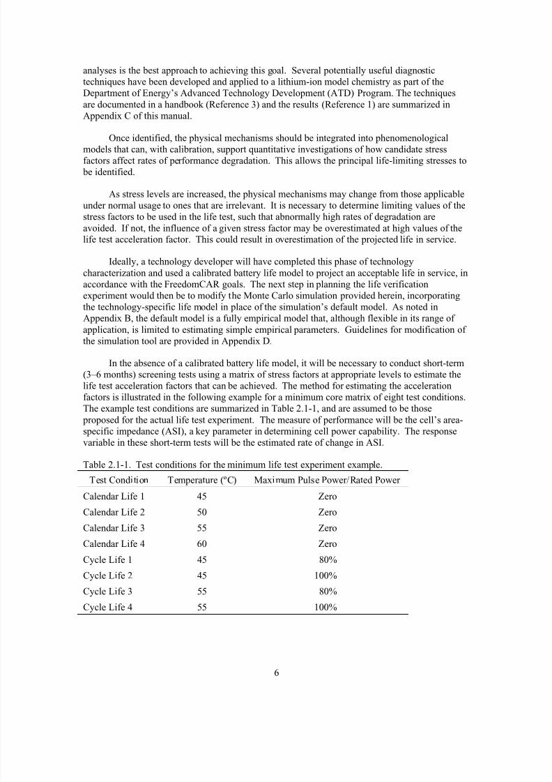
In the absence of a calibrated battery life model, it will be necessary to conduct short-term(3–6 months) screening tests using a matrix of stress factors at appropriate levels to estimate thelife test acceleration factors that can be achieved. The method for estimating the accelerationfactors is illustrated in the following example for a minimum core matrix of eight test conditions.
The example test conditions are summarized in Table 2.1-1, and are assumed to be those proposed for the actual life test experiment. The measure of performance will be the cell’s area-specific impedance (ASI), a key parameter in determining cell power capability. The responsevariable in these short-term tests will be the estimated rate of change in ASI.
Table 2.1-1. Test conditions for the minimum life test experiment example.
Test Condition Temperature (ºC) Maximum Pulse Power/Rated Power
Calendar Life 1 45 Zero
Calendar Life 2 50 Zero
Calendar Life 3 55 Zero
Calendar Life 4 60 ZeroCycle Life 1 45 80%
Cycle Life 2 45 100%
Cycle Life 3 55 80%
Cycle Life 4 55 100%

8/11/2019 Battery Life Verification Test Manual
http://slidepdf.com/reader/full/battery-life-verification-test-manual 19/133
7
Groups of new cells are assumed to be tested at all eight conditions for sufficient durationto yield the average rates of ASI increase shown in Table 2.1-2. Also shown in the table are ratesof change in ASI for samples of aged cells at selected test conditions, where the aged cells haveASI values corresponding to about 80% of the allowable increase in ASI at end of life (EOL).The purpose of testing such aged cells is to estimate the shape of the ASI versus time curve for the technology, as discussed below.
Table 2.1-2. Hypothetical results from short-term tests of new and aged cells.
Measured Rates of Increase in ASI (Ω-cm2/year)
Test Condition New CellsAged Cells
(∆ASI ≈ 4/5 of ∆ASI at EOL)
Calendar Life 1 3.965 (not tested)
Calendar Life 2 5.317 (not tested)
Calendar Life 3 7.059 2.118
Calendar Life 4 9.282 2.785
Cycle Life 1 5.434 (not tested)Cycle Life 2 6.253 (not tested)
Cycle Life 3 9.880 2.964
Cycle Life 4 11.47 3.444
The following simple model was assumed for the purposes of this example:
( ) ( ) ( )
⎥⎦
⎤⎢⎣
⎡
−
−⎟
⎠ ⎞⎜
⎝ ⎛ −+⎟
⎠ ⎞⎜
⎝ ⎛ =
•••
BOL EOL
BOL RATIOCYC CAL REF
ASI ASI
ASI ASI ASI F F ASI ASI 11,0
where ASI
•
is the ASI rate of change estimated from the measured values of ASI, and where the
calendar life and cycle life acceleration factors F CAL and F CYC are assumed to be of the form
1 1
273.15 273.15CAL
ACT REF
T T T
F e
⎡ ⎤⎢ ⎥⎢ ⎥⎣ ⎦
−+ +
=
and
( ) ( )( )[ ]1 1T
RATED
CYC P REF
PK T T
PF K
ω
+ += −⎛ ⎞⎜ ⎟⎝ ⎠
.
Note that F CAL equals 1 when T =T REF and that F CYC equals 1 when P/P RATED=0.
The measured values of ASI •
from Table 2.1-2 imply the following values for the model
parameters, given the reference conditions of T REF = 30ºC, P/P RATED = 0, ASI BOL = 30, and ASI EOL = 40:
REF ASI ,0
• = 1.561 RATIO ASI
• = 0.125 T ACT = 6000 K
K P = 0.5 ω = 2 K T = 0.01/ºC
8/11/2019 Battery Life Verification Test Manual
http://slidepdf.com/reader/full/battery-life-verification-test-manual 20/133
8
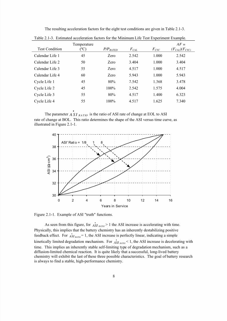
The resulting acceleration factors for the eight test conditions are given in Table 2.1-3.
Table 2.1-3. Estimated acceleration factors for the Minimum Life Test Experiment Example.
Test ConditionTemperature
(ºC) P/P RATED F CAL F CYC
AF =
(F CAL)(F CYC)
Calendar Life 1 45 Zero 2.542 1.000 2.542Calendar Life 2 50 Zero 3.404 1.000 3.404
Calendar Life 3 55 Zero 4.517 1.000 4.517
Calendar Life 4 60 Zero 5.943 1.000 5.943
Cycle Life 1 45 80% 2.542 1.368 3.478
Cycle Life 2 45 100% 2.542 1.575 4.004
Cycle Life 3 55 80% 4.517 1.400 6.323
Cycle Life 4 55 100% 4.517 1.625 7.340
The parameter R A T IO A S I •
is the ratio of ASI rate of change at EOL to ASI
rate of change at BOL. This ratio determines the shape of the ASI versus time curve, asillustrated in Figure 2.1-1.
30
32
34
36
38
40
0 2 4 6 8 10 12 14 16
Years in Service
A S I
( - c m
2 )
ASI' Ratio = 1/8 1 8
Figure 2.1-1. Example of ASI "truth" functions.
As seen from this figure, for RATIO ASI
•
> 1 the ASI increase is accelerating with time.Physically, this implies that the battery chemistry has an inherently destabilizing positive
feedback effect. For RATIO ASI
•= 1, the ASI increase is perfectly linear, indicating a simple
kinetically limited degradation mechanism. For RATIO ASI
•< 1, the ASI increase is decelerating with
time. This implies an inherently stable self-limiting type of degradation mechanism, such as adiffusion-limited chemical reaction. It is quite likely that a successful, long-lived batterychemistry will exhibit the last of these three possible characteristics. The goal of battery researchis always to find a stable, high-performance chemistry.

8/11/2019 Battery Life Verification Test Manual
http://slidepdf.com/reader/full/battery-life-verification-test-manual 21/133
9
Finally, the cells tested in this short-term experiment should be examined using appropriatediagnostic techniques to verify that all cells exhibit the expected physical degradationmechanisms. If cells with the higher acceleration factors show abnormal mechanisms, the limitson the applied stress factors apparently were exceeded. The corresponding test conditions would have to be modified or deleted from the life test experiment.
2.2 Core Life Test Matrix Design Requirements
The minimum life test experiment example described in the previous section is notgenerally expected to provide adequate coverage of the stress factors of probable significance.1
Additional factors such as operating state of charge (SOC), discharge energy throughput rate, and regenerative pulse power versus discharge pulse power may need to be included for a specifictechnology. A more extensive matrix of stress factors and levels is presented in Table 2.2-1. Therationale for selecting these factors and levels is summarized in the following.
Temperature (T) has been shown to be a major stress factor in most battery chemistries. Itis expected that the dependence of the rate of performance degradation on temperature will be of the Arrhenius type. At least three values of temperature would be needed to assess curvature in
the degradation rate with the inverse of absolute temperature. A fourth temperature should beadded if the relevance limit for this factor is uncertain before life verification testing.
State of charge generally affects battery performance, and may have a strong effect on life, particularly at higher values. Battery system requirements for cold-cranking power may dictatethat the minimum operating SOC be relatively high to minimize battery size. The required battery energy rating may then dictate a high maximum operating SOC. Two such levels of operating SOC are suggested to cover the range of possible vehicle application requirements.
The discharge energy throughput rate is expressed in average vehicle speed over theoperating life of the battery—150,000 vehicle miles traveled. The two proposed speedscorrespond to 6,000 and 7,500 hours of battery cycling at 25 and 20 mph, respectively. Thus,
during the battery’s life in service of 15 years, over 14 years will be spent in standby (key-off)mode at open-circuit conditions. This emphasizes the need for thorough calendar life testingwithin the core matrix.
Battery cycling normally will be very dynamic, with frequent high-power discharge and regenerative pulses. Having designed the battery system to meet end of life power ratings, thenormal usage profiles will only stress the battery to some fraction of these ratings. TheFreedomCAR cycle life goals allocate percentages of the total cycles to three levels of fractionalrated power: 80% (240,000) of the 300,000 cycles at 60% of rated power, 15% (45,000) at 80%of rated power, and 5% (15,000) at 95% of rated power. The effects of pulse power levels on the battery’s rate of performance loss may differ between discharge pulses and regenerative pulses.Therefore, independent variation of the power levels for the two types of pulses should be
considered.
1 The screening test approach described in Section 2.1 is not intended to be a substitute for a developer’s detailed technology characterization. It is provided here primarily for use in illustrating how the previously determined lifemodel and acceleration factors are used in the design of the core life test matrix.
8/11/2019 Battery Life Verification Test Manual
http://slidepdf.com/reader/full/battery-life-verification-test-manual 22/133
10
Table 2.2-1. Basic stress factors and suggested stress levels for accelerated battery life testing.
Stress Factor Number of Stress Levels
Suggested Stress Levels
Temperature (°C) 3 High (55–60°C)Medium (50–55°C)
Low (45–50°C)
State of charge (%)(maximum operating)
2 High (80%)Medium (60%)
Discharge energythroughput rate (mph)
3 High (25 mph) Normal (20 mph)Standby (zero)
Fraction of pulse power Rating (%):
Discharge pulsesRegenerative
pulses
22
High (100%), Medium (80%)High (100%), Medium (80%)
The core life test matrix will consist of two parts: a calendar-life matrix and a cycle lifematrix. The recommended calendar-life matrix (see Table 2.2-2) is a 3 x 2 full factorial involvingtemperature and maximum operating SOC.
Table 2.2-2. Recommended calendar life matrix design.
ExperimentCondition Temperature
State of Charge(SOC)
ThroughputRate
Discharge Pulse(Fraction of
Rating)
Charge Pulse(Fraction of
Rating)
1 Low Medium Standby n/a n/a
2 Low High Standby n/a n/a3 Medium Medium Standby n/a n/a
4 Medium High Standby n/a n/a
5 High Medium Standby n/a n/a
6 High High Standby n/a n/a
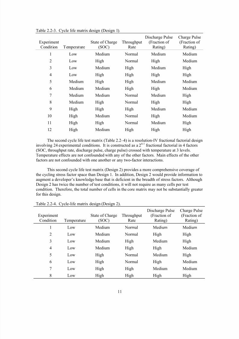
Two possible cycle life matrix designs are given in Tables 2.2–3 and 2.2–4. Each is afractional factorial design in the five stress factors. The first (Table 2.2–3) is a resolution-IIIfractional factorial design involving 12 experimental conditions (Reference 14, page 200). If theintent was to assess the main effects and interactions among the stress factors, then we could separate the main effects from one another with this design. However, main effects would beconfounded with two-factor interactions. This may not be a serious drawback, considering thatthe primary objective of the experiment is to verify the projected life-in-service using a variety of experimental conditions, and not necessarily to model life with the cycling stress factors. Therelative importance of the calendar life testing should be considered in the overall experimentdesign.
8/11/2019 Battery Life Verification Test Manual
http://slidepdf.com/reader/full/battery-life-verification-test-manual 23/133
11
Table 2.2-3. Cycle life matrix design (Design 1).
ExperimentCondition Temperature
State of Charge(SOC)
ThroughputRate
Discharge Pulse(Fraction of
Rating)
Charge Pulse(Fraction of
Rating)
1 Low Medium Normal Medium Medium
2 Low High Normal High Medium
3 Low Medium High Medium High
4 Low High High High High
5 Medium High High Medium Medium
6 Medium Medium High High Medium
7 Medium Medium Normal Medium High
8 Medium High Normal High High
9 High High High Medium Medium
10 High Medium Normal High Medium
11 High High Normal Medium High
12 High Medium High High High
The second cycle life test matrix (Table 2.2–4) is a resolution-IV fractional factorial designinvolving 24 experimental conditions. It is constructed as a 24-1 fractional factorial in 4 factors(SOC, throughput rate, discharge pulse, charge pulse) crossed with temperature at 3 levels.Temperature effects are not confounded with any of the other factors. Main effects of the other factors are not confounded with one another or any two-factor interactions.
This second cycle life test matrix (Design 2) provides a more comprehensive coverage of the cycling stress factor space than Design 1. In addition, Design 2 would provide information to
augment a developer’s knowledge base that is deficient in the breadth of stress factors. AlthoughDesign 2 has twice the number of test conditions, it will not require as many cells per testcondition. Therefore, the total number of cells in the core matrix may not be substantially greater for this design.
Table 2.2-4. Cycle-life matrix design (Design 2).
ExperimentCondition Temperature
State of Charge(SOC)
ThroughputRate
Discharge Pulse(Fraction of
Rating)
Charge Pulse(Fraction of
Rating)
1 Low Medium Normal Medium Medium
2 Low Medium Normal High High
3 Low Medium High Medium High
4 Low Medium High High Medium
5 Low High Normal Medium High
6 Low High Normal High Medium
7 Low High High Medium Medium
8 Low High High High High

8/11/2019 Battery Life Verification Test Manual
http://slidepdf.com/reader/full/battery-life-verification-test-manual 24/133
12
ExperimentCondition Temperature
State of Charge(SOC)
ThroughputRate
Discharge Pulse(Fraction of
Rating)
Charge Pulse(Fraction of
Rating)
9 Medium Medium Normal Medium Medium
10 Medium Medium Normal High High
11 Medium Medium High Medium High
12 Medium Medium High High Medium
13 Medium High Normal Medium High
14 Medium High Normal High Medium
15 Medium High High Medium Medium
16 Medium High High High High
17 High Medium Normal Medium Medium
18 High Medium Normal High High
19 High Medium High Medium High20 High Medium High High Medium
21 High High Normal Medium High
22 High High Normal High Medium
23 High High High Medium Medium
24 High High High High High
2.3 Core Life Test Matrix Design and Verif ication
Design and verification of the core life test matrix is conducted in three stages. In the firststage, a preliminary experiment design is developed by selecting the stress factors, stress levels,and number of test conditions in the matrix. The acceleration factor (AF) expected for each testcondition is used to obtain values of expected life on test, which in turn are used to obtainexpected uncertainties in life on test, based on expected uncertainties due to cell-to-cellmanufacturing variations and ASI measurement errors. A target level is selected such that the projected life in service will be achieved with 90% confidence. An estimate is made of the totalnumber of cells required in the core matrix to demonstrate the target projected life in service with90% confidence. This estimate is made in conjunction with a preliminary allocation of the cellsto each test condition (performed with the use of “Cell Allocator.xls”), such that the confidence ismaximized for that total number of cells. This stage is described more fully in Section 2.3.1.
In the second stage, the Battery Monte Carlo Simulation tool (“Battery MCS.xls”) is used
to adjust and verify the preliminary design from the first stage. This is done by simulating the lifetest—generating simulated ASI measurements with random variations in the cells’ performanceand in the ASI measurements. These simulated data are analyzed as though they were from anactual test. The simulation is repeated for about 100 trials for each test condition to obtainestimates for the uncertainty in the estimated lives on test. The simulation results are used toshow that the target confidence level selected can be achieved with the candidate matrix design.If the results are not as expected—primarily because the simulation-generated uncertainties in theestimated lives on test do not agree with the preliminary estimates—the number of cells and cell

8/11/2019 Battery Life Verification Test Manual
http://slidepdf.com/reader/full/battery-life-verification-test-manual 25/133
13
allocations will have to be iterated until an acceptable design is obtained. This stage is described more fully in Section 2.3.2.
The third and final stage is reverification of the matrix design using test data from theinitial characterization of the actual test cells. The primary objective is to verify that the test cellsand test facilities have achieved the desired levels of repeatability and accuracy assumed in the
original matrix design process. Simple analysis of the characterization data for ASI at the twoSOC values can separate the effects of cell-to-cell variation from ASI measurement noise. Also,in-process data from the cell manufacturing operations can be used to estimate the variability incell performance. If the noise estimates from these initial test data are significantly different fromthose assumed in the original experiment design, the design may need to be altered to achieve anacceptable level of confidence in the projection of minimum life in service. This stage isdescribed more fully in Section 2.3.3.
2.3.1 Preliminary Design Stage
As discussed below, the preliminary design of the core life test matrix begins with theexpected values of life on test, from whence estimated values of life on test and their associated
uncertainties are developed.
2.3.1.1 Expected Lives on test
Life verification testing of a mature technology will be based on a calibrated phenomenological model that predicts successful achievement of the FreedomCAR life goals.Such a model will be used to obtain expected AF values for the core matrix of test conditions and the corresponding expected lives on test:
LTEST = LCAL / AF
where AF = (F CAL ) (FCYC) and where the calendar life is related to the life in service by LSERV = LCAL / F CYC,NOM .
For the default empirical model of Appendix A, calendar life is found by integrating theASI rate of change and solving the result for the allowable power fade (PF ) with F CAL = F CYC = 1:
( )( )
( ) ⎟ ⎠ ⎞⎜
⎝ ⎛ −⎟
⎠ ⎞⎜
⎝ ⎛ −
⎟ ⎠ ⎞⎜
⎝ ⎛
=••
•
11
ln
,0 RATIO REF
RATIO BOL
ASI ASI PF
ASI ASI PF
CAL L .
Assuming that the phenomenological model is perfectly accurate, these expected lives ontest would be the actual results of the life tests, in the absence of any cell-to-cell variation or ASImeasurement error. For the default empirical model of Appendix A, the data analysis would yield the following “true” values of the three model parameters:
( )1
1/ K
RATIO
EOL ASI β
•
=
( ) ( )1 0
0
11
1
1
RATIO
RATIO
ASI ASI PF
ASI
β
β
•
•
− −−
−
⎡ ⎤⎢ ⎥⎣ ⎦=

8/11/2019 Battery Life Verification Test Manual
http://slidepdf.com/reader/full/battery-life-verification-test-manual 26/133
14
ASI O = ASI BOL = 30 Ω-cm2 for the present example
where K EOL = LTEST / ∆t RPT . (∆t RPT is the RPT interval, 4/52 years for the example.)
The corresponding values of ASI would then be:
( )( )
K
K
K ASI ASI 10
1
10
11 β
β β β +
−−=
where K = t / ∆t RPT is the test interval index running from K = 0 to K = K EOT = t EOT / ∆t RPT .
For the simple model assumed for the design example in Section 2.1, the value for thecycle life acceleration factor under nominal conditions of normal usage is:
( ) ( ) ( ) ( ) ( ) ( ) ( ), 1 0.8 0.6 0.15 0.8 0.05 0.95 15CYC NOM PF K ω ω ω ⎡ ⎤= + + +⎣ ⎦
≈ 1.014 for the numerical values of K P and ω from Section 2.1.
Note that the allowable power fade is assumed to be 25% of the beginning of life pulse power capability for this example. Also, one equivalent year of battery operation has been assumed over its 15-year life in service. Also implied in this equation is that calendar and cycle life effects are
path independent. This assumption is included in the recommended list of supplemental life tests.The implied calendar life is about 15.22 years.
Then, from Table 2.1-3, the values for AF at each test condition give the expected lives ontest and “true” model parameters, as shown in Table 2.3-1.
Table 2.3-1. Expected lives on test for the Minimum Life Test Experiment example.
Test Condition Temperature
(ºC) P/P RATED AF
LTEST
(y)
ßo
(ohm-cm2
) ß1
Calendar Life 1 45 Zero 2.542 5.99 1.092 0.9736
Calendar Life 2 50 Zero 3.404 4.47 1.456 0.9648
Calendar Life 3 55 Zero 4.517 3.37 1.920 0.9536
Calendar Life 4 60 Zero 5.943 2.56 2.509 0.9394
Cycle Life 1 45 80% 3.478 4.38 1.486 0.9641
Cycle Life 2 45 100% 4.004 3.80 1.708 0.9588
Cycle Life 3 55 80% 6.323 2.41 2.660 0.9358
Cycle Life 4 55 100% 7.340 2.07 3.081 0.9256
2.3.1.2 Estimated Lives on test
In the simulation, as in reality, the true performance of the test cells is corrupted by “noise”associated with cell-to-cell variations and ASI measurement errors. The data analysis model thuscan provide only estimates of the three key fitting parameters:
0ˆ β = estimated value of β O
8/11/2019 Battery Life Verification Test Manual
http://slidepdf.com/reader/full/battery-life-verification-test-manual 27/133
15
1ˆ β = estimated value of β 1
0 I S A = estimated value of ASI O .
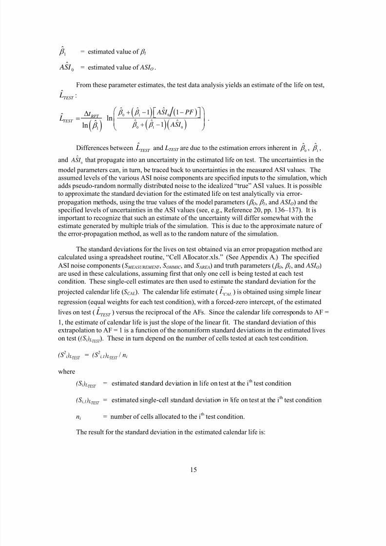
From these parameter estimates, the test data analysis yields an estimate of the life on test,
TEST L :
( )( ) ( )
( ) ( )0 1 0
0 1 01
ˆ ˆ ˆ1 1
ˆ ˆ ˆ1ˆ ln
ˆln
RPT TEST
ASI PF
ASI
t L
β β
β β β
+ − −
+ −
⎛ ⎞⎡ ⎤∆ ⎣ ⎦⎜ ⎟=⎜ ⎟⎝ ⎠
.
Differences between TEST L and LTEST are due to the estimation errors inherent in0
ˆ β ,1
ˆ β ,
and0
ˆ ASI that propagate into an uncertainty in the estimated life on test. The uncertainties in the
model parameters can, in turn, be traced back to uncertainties in the measured ASI values. Theassumed levels of the various ASI noise components are specified inputs to the simulation, whichadds pseudo-random normally distributed noise to the idealized “true” ASI values. It is possibleto approximate the standard deviation for the estimated life on test analytically via error-
propagation methods, using the true values of the model parameters ( β O, β 1, and ASI O) and thespecified levels of uncertainties in the ASI values (see, e.g., Reference 20, pp. 136–137). It isimportant to recognize that such an estimate of the uncertainty will differ somewhat with theestimate generated by multiple trials of the simulation. This is due to the approximate nature of the error-propagation method, as well as to the random nature of the simulation.
The standard deviations for the lives on test obtained via an error propagation method arecalculated using a spreadsheet routine, “Cell Allocator.xls.” (See Appendix A.) The specified ASI noise components (S MEASUREMENT , S OHMIC , and S AREA) and truth parameters ( β O, β 1, and ASI O)are used in these calculations, assuming first that only one cell is being tested at each testcondition. These single-cell estimates are then used to estimate the standard deviation for the
projected calendar life (S CAL). The calendar life estimate ( CAL L ) is obtained using simple linear
regression (equal weights for each test condition), with a forced-zero intercept, of the estimated
lives on test ( TEST L ) versus the reciprocal of the AFs. Since the calendar life corresponds to AF =
1, the estimate of calendar life is just the slope of the linear fit. The standard deviation of thisextrapolation to AF = 1 is a function of the nonuniform standard deviations in the estimated liveson test ((S i) LTEST
). These in turn depend on the number of cells tested at each test condition.
(S 2i) LTEST
= (S 2i,1) LTEST
/ ni
where
(S i) LTEST = estimated standard deviation in life on test at the ith test condition
(S i,1) LTEST = estimated single-cell standard deviation in life on test at the ith test condition
ni = number of cells allocated to the ith test condition.
The result for the standard deviation in the estimated calendar life is:

8/11/2019 Battery Life Verification Test Manual
http://slidepdf.com/reader/full/battery-life-verification-test-manual 28/133
16
( ) ( )
( )
2 2
2
1/
1/
TEST i i
L
CAL
i
AF S
S AF
= ∑
∑.
If weighted linear regression is used (weights inversely proportional to
( )
2
TEST i
L
S ) to
estimate α in the model ⎟ ⎠ ⎞
⎜⎝ ⎛ ⋅= AF
L1
α , then the standard error of α ˆ is
( )
( ) ( ) ( )1 2
2 2 2 2 2 21 1 2 2
1ˆ. .
TEST TEST TEST
m
m m L L L
S E nn n
S AF S AF S AF
α =+ + +
⋅ ⋅ ⋅…
.
Suppose that for the example design (with an expected life in service of 15 years) we desireto show that the life in service is at least 13.5 years (10% less than expected) with 90%confidence. The corresponding calendar life must exceed 13.85 years with 90% probability. The
expected calendar life of 15.22 years allows a standard deviation in calendar life of
SCAL = (15.22 – 13.85)/1.415 = 0.97 years
where 1.415 is the 90th percentile of the t-distribution with (8–1) degrees of freedom.
Using the “Cell Allocator.xls” tool gives the results shown in Table 2.3-2. The totalnumber of cells chosen for this example design to obtain this value of S CAL is 148. A minimum of 4 cells was specified for any one test condition. The assumed test duration was 2 years, with ASImeasurements taken every 4 weeks. Also in this example, the assumed standard deviations for the three components of “noise” in the ASI data were as follows: (a) cell-to-cell fixed ohmicvariation = 1%, (b) cell-to-cell electrode area variation = 0.5%, and (c) ASI measurement error =
1%.
Table 2.3-2. Preliminary allocation of cells for the Minimum Life Test Experiment example.
TestCondition
Temperature(°C) P/P RATED AF LTEST (S i,1) LTEST
ni (S i) LTEST
Calendar Life 1 45 Zero 2.542 5.99 7.87 72 0.927
Calendar Life 2 50 Zero 3.404 4.47 3.01 24 0.614
Calendar Life 3 55 Zero 4.517 3.37 1.26 8 0.445
Calendar Life 4 60 Zero 5.943 2.56 0.71 4 0.354
Cycle Life 1 45 80% 3.478 4.38 2.80 24 0.572
Cycle Life 2 45 100% 4.004 3.80 1.79 8 0.633
Cycle Life 3 55 80% 6.323 2.41 0.65 4 0.326
Cycle Life 4 55 100% 7.340 2.07 0.56 4 0.278
It is possible to generalize the results displayed in Table 2.3–2 to provide additionalguidance. First, the total number of cells required to meet a target level of uncertainty in theestimated calendar life and life in service is inversely proportional to the square of the target

8/11/2019 Battery Life Verification Test Manual
http://slidepdf.com/reader/full/battery-life-verification-test-manual 29/133
17
standard deviation. Thus, the results of any one allocation can be easily scaled to obtain the totalnumber of cells for an alternative target standard deviation. Second, allocation of replicate cellsto the various test conditions should be weighted toward the lower AF values. The reason for thisis that the “signal” of ASI growth is reduced as AF is decreased. The noise is approximatelyconstant (within statistical fluctuations), and therefore the signal/noise ratio is decreasing. Thenoise must be correspondingly reduced to compensate for this by using more cells to estimate the
life on test. Third, other calculations have shown that there is negligible advantage to morefrequent ASI measurement. Finally, the number of cells may be reduced by extending theduration of testing. However, this adds to the cost of testing and delays the commercializationdecision. Conversely, testing more cells could shorten the test duration, but not significantly,depending on the limitations of existing test facilities.
2.3.2 Final Design Stage
The battery Monte Carlo Simulation (MCS) tool is used at this stage to verify that the totalnumber of cells and their preliminary allocation to the test conditions provide the desired 90%lower confidence limit in the projected life in service. Key inputs to the simulation are true
calendar life, ASI •
ratio, test duration, RPT measurement interval, allowable power fade at end of
life, and three components of noise in the ASI data. The noise components are specified as percentages of the initial ASI at beginning of life. They include variations in the cell electrodearea and fixed ohmic resistance due to manufacturing process variations. The third noise sourceis ASI measurement error from test equipment limitations. The ASI at beginning of life is anarbitrary input that does not affect the predicted life but can be used to match the value of actualcells if desired.
The acceleration factor and number of cells are variable inputs to the simulation for eachtest condition. Finally, the number of trials for each test condition is specified. This willgenerally be the same for all test conditions and should be sufficient to obtain good estimates of the standard deviation of life on test. For example, consider normally distributed randomvariables with standard deviation, σ. About 90% of the time, the observed standard deviation
based on a sample of size 100 from that distribution will be within about 10% of σ. The resultsof these calculations for the experiment design example are summarized in Table 2.3-3, where100 trials were used for each test condition.
Table 2.3-3. Simulation results for the Minimum Life Test Experiment example.
Life on test (y) Standard Deviation (y)
Test Condition Temperature P/P RATED ni TrueMCS
Estimate (S i) LTEST
MCSEstimate
Calendar Life 1 45 Zero 72 5.99 5.98 0.927 0.721
Calendar Life 2 50 Zero 24 4.47 4.55 0.614 0.502
Calendar Life 3 55 Zero 8 3.37 3.46 0.446 0.374
Calendar Life 4 60 Zero 4 2.56 2.63 0.354 0.282
Cycle Life 1 45 80% 24 4.38 4.43 0.572 0.565
Cycle Life 2 45 100% 8 3.80 3.90 0.633 0.669
Cycle Life 3 55 80% 4 2.41 2.45 0.326 0.260
Cycle Life 4 55 100% 4 2.07 2.08 0.278 0.166
8/11/2019 Battery Life Verification Test Manual
http://slidepdf.com/reader/full/battery-life-verification-test-manual 30/133
18
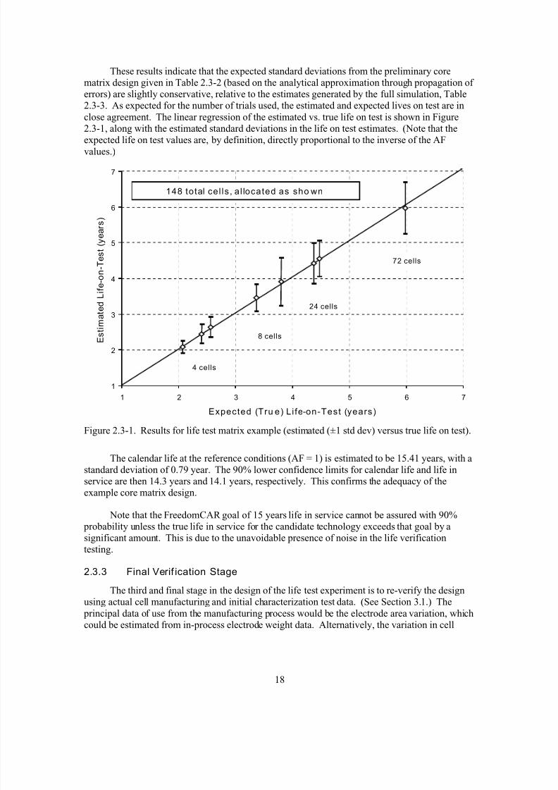
These results indicate that the expected standard deviations from the preliminary corematrix design given in Table 2.3-2 (based on the analytical approximation through propagation of errors) are slightly conservative, relative to the estimates generated by the full simulation, Table2.3-3. As expected for the number of trials used, the estimated and expected lives on test are inclose agreement. The linear regression of the estimated vs. true life on test is shown in Figure2.3-1, along with the estimated standard deviations in the life on test estimates. (Note that the
expected life on test values are, by definition, directly proportional to the inverse of the AFvalues.)
1
2
3
4
5
6
7
1 2 3 4 5 6 7
Expected (Tru e) L i fe-on-Test (years)
E s t i m a t e d L i f e - o
n - T e s t ( y e a r s )
72 cells
24 cells
8 cells
4 cells
148 total cel ls , a l located as sho wn
Figure 2.3-1. Results for life test matrix example (estimated (±1 std dev) versus true life on test).
The calendar life at the reference conditions (AF = 1) is estimated to be 15.41 years, with astandard deviation of 0.79 year. The 90% lower confidence limits for calendar life and life inservice are then 14.3 years and 14.1 years, respectively. This confirms the adequacy of theexample core matrix design.
Note that the FreedomCAR goal of 15 years life in service cannot be assured with 90% probability unless the true life in service for the candidate technology exceeds that goal by asignificant amount. This is due to the unavoidable presence of noise in the life verification
testing.
2.3.3 Final Verif ication Stage
The third and final stage in the design of the life test experiment is to re-verify the designusing actual cell manufacturing and initial characterization test data. (See Section 3.1.) The
principal data of use from the manufacturing process would be the electrode area variation, whichcould be estimated from in-process electrode weight data. Alternatively, the variation in cell

8/11/2019 Battery Life Verification Test Manual
http://slidepdf.com/reader/full/battery-life-verification-test-manual 31/133
19
capacity from the initial characterization tests could be used as an approximation to the electrodearea variation.
The ASI measurements from the initial characterization tests are analyzed to verify that thecell-to-cell variations and ASI measurement errors are as expected. Each life test cell will havetwo ASI measurements to be used in this analysis—both at the 30ºC reference temperature. The
ASI measurements will be adjusted on the basis of the variation in the actual cell temperatures,relative to the nominal temperatures. The measured ASI temperature sensitivity for the cells will
be used to make these adjustments (see Appendix B).
As presented in more detail in Section 4.1, the cells’ ASI data are plotted such that thevalues at the maximum SOC are on the X-axis and the corresponding values at the minimumSOC are on the Y-axis. Ideally, these data will fall on a single straight line with no variationfrom cell to cell. In practice, there will be scatter about the line. The cell-to-cell variation can bedistinguished from the measurement-to-measurement variation by variance components analysis.In the event that the magnitude of the estimated cell-to-cell variations and ASI measurementerrors do not agree with the values assumed in the original design of the experiment, the series of 100-trial simulations should be rerun with the new estimates.
The results of this analysis may indicate that corrective actions are required to achieve thegoals of the life test experiment. Such actions could include the following:
1. Upgrading the test facilities/test procedures to reduce ASI measurement error.
2. Adding cells to one or more of the test conditions.
3. Extending the test duration, especially for test conditions with the longest expected lives ontest.
4. Culling of cells from the population to reduce the cell-to-cell variation, and manufacturingadditional cells to populate the core and supplemental matrices.
2.4 Supplemental Life Test Matrix Design Requirements
The primary objective of supplemental life testing (where used) is to confirm the validityof assumptions that are made in defining the core life test matrix, typically in order to reduce thecore matrix to a manageable size. Each such assumption can be assessed experimentally bycomparison with a result from the core life test matrix. The following assumptions are considered to be the most likely to need such confirmation:
1. The future state of health (SOH) of a cell depends only on the present SOH and futurestresses, independent of the path taken to reach the present SOH.
2. Cold-start operation (i.e., cold cranking) does not have an adverse effect on cell life.
3. Low-temperature operation, within accepted performance constraints, does not have anadverse effect on cell life.
For each of these assumptions, a corresponding experimental plan is described in thefollowing sections. In all cases, the assumptions are posed as null hypotheses to be assessed at anacceptable level of Type I error. The Type I error is the probability that the null hypothesis isrejected when it is in fact true. The appropriate analyses of the supplemental test results aredescribed later in Section 4.

8/11/2019 Battery Life Verification Test Manual
http://slidepdf.com/reader/full/battery-life-verification-test-manual 32/133
20
Additionally, a small group of selected cells (typically four) will be subjected to the sametest conditions as one of the high AF groups of the core life test matrix, except that these cellswill use the full HPPC test for their RPT regime. Data from these cells will be used to identifyand isolate possible aging effects on the shape of the pulse power capability curve for aging cells.
No formal hypothesis testing is involved, and a detailed experimental plan is not provided for thisgroup of cells.
2.4.1 Experimental Plan to Assess Path Independence
The null hypothesis for this supplemental test is: the rate of change in ASI depends only onthe present value of ASI and the applied stress factors, not on the history of use that resulted inthe present value of ASI.
The experimental plan is to conduct combined calendar life and cycle life test regimes ontwo groups of cells in alternate sequences of exposure to the regimes. For example, the plan for this test corresponding to the minimum core life test matrix example of Section 2.3 would be totest alternately in the Calendar Life 3 test condition (T = 55ºC) and in the Cycle Life 4 testcondition (T = 55ºC, P/P RATED = 100%). One group would be tested in the cycle life regime until
it had reached about half of its expected ASI increase for that regime, and then switched to thecalendar life regime. The second group would be started on the calendar life regime and switched to the cycle life regime at the same ASI increase as the switchover for the first group. Theswitchover of the second group would occur at a later time than the switchover for the first group.The ASI data for the two groups, measured at the same frequency as for the core matrix life tests,would be compared to the ASI data for cells in the core life test matrix under the same conditions.
The criterion for rejecting the null hypothesis would be based on statistically significantdifferences in the ASI rates of change among the four groups. In the core matrix example designin Section 2.3, eight cells were allocated to the Calendar Life 3 condition and four cells to theCycle Life 4 condition. Comparable numbers of cells would be used in the correspondingsupplemental tests.
Selection of specific test conditions to use in making the comparison with the core matrixtest results involves tradeoffs of relative ASI degradation “signal” versus the “noise” (standard deviation) in the estimated ASI degradation. High acceleration factors provide good signal tonoise, but the differences between the core matrix and supplemental matrix values of life on testmay be easier to detect for lower total ASI degradation. Such a tradeoff should be evaluated for any proposed supplemental test condition.
2.4.2 Experimental Plan to Assess Cold-Start Operation
The null hypothesis for this supplemental test is that periodic cold cranking does notadversely affect battery life.
It will not be practical to duplicate the significant number of cold starts that may berequired of the vehicle in the most extreme climates in which it is to be marketed. Instead, twosupplemental groups of cells will be tested in the cold cranking regime as part of their periodicreference performance test (RPT). Otherwise their RPT will be the same as for the correspondinggroups in the core matrix. To maximize the possible interactive effects of cold-cranking on life,the test conditions for these two supplemental groups would be the same as for the core matrixcells in the Calendar Life 3 and Cycle Life 4.

8/11/2019 Battery Life Verification Test Manual
http://slidepdf.com/reader/full/battery-life-verification-test-manual 33/133
21
In a two-year test duration, this would imply only 27 cold-cranking tests for these cells.However, the expected increases in ASI for these cells would be near the maximum, thusallowing an assessment of how the performance degradation correlates with degradation in cold-cranking capability. More frequent cold-cranking tests could be used for these groups, but itcould make a direct comparison with the corresponding core matrix cells more difficult.Appropriate numbers of cells for these groups would be the same as for the core matrix cells with
the same expected lives on test.
The criterion for rejecting the null hypothesis would be based on statistically significantdifferences in the ASI increases over the test duration among the four groups.
2.4.3 Experimental Plan to Assess Low-Temperature Operation
The null hypothesis for this supplemental test is that battery operation at low temperaturesdoes not adversely affect battery life.
This supplemental test is unique in that the test conditions cannot be matched to any of thecore matrix test conditions. For that reason, the conditions for the test need to be reasonably
extreme to detect any enhanced ASI increase. On the other hand, any failure mechanismassociated with low-temperature operation should be well understood before life verificationtesting. If operating limits have been identified to avoid adverse effects on life, the test would beconducted at those limits (e.g., maximum operating SOC, but limited regenerative pulse power).One possible plan is to use two groups of cells, one control group operating well within thespecified limits, and one operating exactly at the limits. The number of cells in each group would have to be determined on the basis of the acceptable error in rejecting the null hypothesis when itshould be accepted. As with the other test conditions, the criterion for rejection would be based on a comparison of the ASI increases for the two groups. A further criterion could also be theabsence of any physical diagnostic evidence showing that the two groups experienced differentlow-temperature failure mechanisms. If this is included in the hypothesis test, the number of cellscould be minimized for this part of the supplemental matrix. No fewer than four cells per groupwould be recommended in any case.
8/11/2019 Battery Life Verification Test Manual
http://slidepdf.com/reader/full/battery-life-verification-test-manual 34/133
22
3. LIFE TEST PROCEDURES
Successful battery technology life verification will require careful implementation of the procedures specified in this section. The procedures described in the following sections aregrouped into initial characterization (Section 3.1), core matrix life test (Section 3.2), and supplemental life test (Section 3.3). Several performance test procedures are incorporated byreference to existing FreedomCAR battery test manuals. Test facility measurement and datarecording requirements are provided in Appendix E. It is assumed throughout that the test articlesare individual battery cells sized to meet the performance ratings of at least one FreedomCAR
battery system target application.
The initial cell characterization tests fall into two categories: basic tests applied to all cellsand additional tests applied only to selected cells. Basic tests, all conducted at the nominalreference temperature of 30ºC, include (a) capacity verification at a nominal C/1 discharge rate;and (b) pulse power verification using a minimum pulse power profile at only two states of charge. Additional characterization tests on selected cells, for all temperatures to be used in thelife tests, include (a) open-circuit voltage measurement versus state of charge, (b) pulse power verification using the standard hybrid pulse power characterization (HPPC) procedure, (c) self-
discharge, (d) cold-cranking power verification (low temperature only), and (e) ACelectrochemical impedance spectral analysis. Cells receiving the additional characterization testswill not be used in the core life test matrix, and may be used only selectively in the supplementallife test matrix.
Core matrix life tests include both calendar/standby at open-circuit and cycling tests atvarious levels of pulse power relative to the cell rated power. All core matrix tests are conducted at elevated temperature, with periodic reference performance tests (RPTs) at the nominalreference temperature. The RPTs for the core matrix will be limited to application of theminimum pulse power characterization (MPPC) profile at two states of charge at the testtemperature and the reference temperature. The states of charge will correspond to the maximumand minimum values intended for normal battery operation, as defined by the corresponding
open-circuit voltages. The RPT will include measurement of the available capacity (at C/1 rate) between the two limiting states of charge.
Three types of supplemental life test are envisioned as part of the overall technology lifeverification program. They include (a) combined calendar and cycle life, (b) periodic verificationof cold-cranking power, and (c) verification of low-temperature operation. Results from thesesupplemental tests will be compared with core matrix test results to assess the effects, if any, of the supplemental test conditions on the projected life in service for the candidate technology.
3.1 Initial Characterization Tests
The objectives of the initial cell characterization are to (1) establish the appropriate test
parameters consistent with accepted technology limitations and requirements for the targetapplication, (2) verify the initial capabilities of the life test cells, and (3) verify the readiness of the test facilities to meet the data acquisition requirements of the program. Although the twocategories of characterization testing are presented first for all cells, followed by tests for onlyselected cells, they will be conducted in a logical sequence to provide the appropriate flow of information from one test to the next.
This manual primarily deals with life testing and the associated reference performancetesting. The minimum regime of initial characterization tests is also described. Note that such
8/11/2019 Battery Life Verification Test Manual
http://slidepdf.com/reader/full/battery-life-verification-test-manual 35/133
23
tests are generally application dependent. The test procedures specified in the following are based on the power assist application and should be modified appropriately for life testingdirected at other applications (References 8-11).
3.1.1 General Test Condit ions and Scaling
Certain standard checks should be made of all cells in their as-received condition to ensurethat the cells have not been damaged in shipment to the test facility. These checks will minimallyinclude (a) visual inspection for damage, (b) measurement of open-circuit voltage, and (c) areference measurement of AC impedance at 1 kHz. All cells should also be weighed on receipt.
A life test regime must establish and maintain a consistent set of conditions under whichtests are conducted. These include device environment (primarily temperature), test limitationsimposed by either the application or the device under test, and the appropriate scaling of testloading for the target application.
Accurate temperature control and measurement is especially important during the reference performance tests because they are used to track performance changes over time, which are the
basis for verification of life. The default temperature for the characterization and reference performance tests specified in this manual is the reference temperature of 30ºC. All testingshould be conducted using environmental chambers.
Operating limits for the test articles may vary between target applications, and may includetechnology-specific constraints. In this manual, such limits are assumed to be controlled asrequired to meet the objectives of the life verification testing, and implemented in modified test
procedures as appropriate.
The allowable operating voltage range (and by implication the allowable state of chargerange) for a device is established by the manufacturer. For purposes of this manual, anapplication-specific operating range (that may be a subset of this allowable range) is specified,typically in a test plan for the life test program. This range extends from SOCMAX to SOCMIN, and the standard MPPC reference testing for all cells is conducted over this range. In addition tomanufacturer operating limits, the following guidelines should be considered for choosing thesetest limits: (a) SOCMAX should generally be equal to the maximum test SOC used in the core lifetest matrix; (b) SOCMIN can be equal to the minimum test SOC used in the core life test matrix,
provided that the MPPC pulse profile at SOCMAX will not bring the SOC below this value.(Otherwise SOCMIN will need to be a lower value to avoid the need to recharge the cell before thesecond pulse profile can be performed.) During life testing, these SOC values are not measured directly; instead the corresponding open circuit voltages are used to represent them. (See theGlossary for more information on SOCMAX and SOCMIN.)
Scaling of test loads is necessarily done using the methods defined for the targetapplication, so that performance can fairly be compared to the application goals. Test power
levels for devices targeted to power assist applications are scaled using a “battery size factor”(BSF) which is defined as “the minimum number of cells or modules expected to be required tomeet all the FreedomCAR performance and life goals.” The determination and use of the BSF isdescribed in detail in Reference 8. The minimum characterization tests for all cells described inthis manual do not depend on such application-based scaling, although cycle life test profiles areapplication-specific.

8/11/2019 Battery Life Verification Test Manual
http://slidepdf.com/reader/full/battery-life-verification-test-manual 36/133
24
3.1.2 Minimum Characterization for All Cells
Two basic characterization tests will be conducted for all cells in the overall lifeverification program: (1) verification of rated capacity at the C/1 rate and (2) verification of pulse
power capabilities at the minimum and maximum SOCs. Both tests will be conducted only at thereference temperature.
3.1.2.1 Capacity Verification
The static capacity test will consist of (a) a recharge to 100% SOC, using themanufacturer’s recommended procedure, (b) a one-hour rest at open-circuit, and (c) a constant-current discharge at C/1 rate to the manufacturer’s recommended cutoff voltage. This sequencewill be repeated a minimum of three times until three successive discharge capacities agreewithin a total spread of 2%.
3.1.2.2 Pulse Power Verification (MPPC)
Initial verification of all cells’ pulse power capabilities will be done using the followingminimum pulse power characterization (MPPC) procedure. This test is an abbreviated version of
the low current hybrid pulse power characterization (HPPC) test described in Reference 8. Thecurrent-based pulse profile used for the MPPC is identical to that for the HPPC. For power assistapplications, pulse currents are 5C and 3.75C for the 10-second discharge and regenerative
pulses, respectively, which are separated by a 40-second rest interval.
The MPPC sequence is as follows:
1. The cell is recharged at a maximum rate of C/1 to the maximum SOC (SOCMAX), based onthe corresponding open-circuit voltage (OCV) determined from the OCV versus SOCcharacterization test described in Section 3.1.3.1 below. A taper current is used tocomplete the recharge to the specified OCV, within the limit of a specified minimum taper current. (See Section 3.1.1 and the Glossary for more information on SOCMAX and SOCMIN.)
2. The cell is allowed to rest at open-circuit for one hour.
3. The specified MPPC profile is applied, followed by discharge at the maximum rate of C1/1to the minimum SOC (SOCMIN). A taper current is used to complete the discharge to thecorresponding specified minimum OCV.
4. The cell is allowed to rest at open-circuit for one hour.
5. The specified MPPC profile is applied.
3.1.3 Addi tional Characterization of Selected Cells
Additional characterization tests will be conducted on a limited number of cells to meet thefollowing objectives: (1) mapping of OCV versus SOC to determine the OCVs that correspond to
the specified minimum and maximum SOCs, (2) verification of pulse power capabilities over thefull range of cell SOC using the HPPC procedure, (3) verification of self-discharge rates, (4)verification of cold-cranking power capabilities, and (5) initial measurement of ACelectrochemical impedance spectra (EIS) for comparison with end-of-test spectra. Theseadditional tests will be conducted at all specified test temperatures to be used in the core life-testmatrix, including the reference temperature. Recommendations for numbers of cells for each of these additional tests are provided in the following.

8/11/2019 Battery Life Verification Test Manual
http://slidepdf.com/reader/full/battery-life-verification-test-manual 37/133
25
3.1.3.1 Open-circuit Voltage versus State of charge
The procedure to measure OCV versus SOC is as follows:
1. Recharge the cell to 100% SOC using the manufacturer’s recommended procedure.
2. Allow the cell to rest at open-circuit for a minimum of one hour, or until the voltage has
reached a stable condition. (See the Glossary for information.)3. Discharge the cell at a maximum rate of C/1 for a specified fraction (e.g., 5%) of the rated
capacity.
4. Allow the cell to rest at open-circuit for a minimum of one hour, or until the voltage hasreached a stable condition.
5. Repeat steps 3 and 4 above until the manufacturer’s recommended minimum dischargevoltage is reached.
This test should be conducted on a minimum of two cells at each temperature.
3.1.3.2 Pulse Power Verification
The HPPC procedure of Reference 8 (for power assist applications) will be used to verifythe cells’ pulse power capabilities over the full range of SOC. In addition to the normallyspecified values of SOC used in this test, the HPPC profile should also be applied at theminimum and maximum specified SOCs. (This may require a separate test in some cases.) Toenable comparison of these results with those obtained using the MPPC, a minimum of eight cellsshould be tested at each temperature to be used for life testing.
3.1.3.3 Self-discharge Rate Characterization
The self-discharge test of Reference 8 will be used to estimate the rate of cell self-discharge from SOCMAX as a function of test temperature. The normal test duration of one week may be reduced for any cells that reach SOCMIN prior to the end of this test. A minimum of two
cells is recommended for each test temperature. (This testing may be considered optional for celldesigns whose self-discharge behavior is already well-characterized, since the general behavior isalso observable during calendar life testing.)
3.1.3.4 Cold-cranking Power Verification
Depending on the target application, the cold-cranking test procedure of the appropriateFreedomCAR manual (References 8-11) will be conducted on all cells selected for thesupplemental test conditions of Section 2.4.2. The appropriate cold-cranking power profile will
be applied at both the maximum and minimum SOCs. Note that the same test procedure will beused in the periodic RPTs applied to the cells of the cold-cranking portion of the supplementallife-test matrix (Section 3.3.2).
3.1.3.5 AC Electrochemical Impedance Spectrum (EIS) Testing
An initial full-spectrum sweep of AC complex impedance (as defined in a cell-specific test plan) will be conducted only for the cells to be life tested in the supplemental life-test matrix.Results from this beginning of life characterization will be compared to results obtained for allcells (from both supplemental and core matrices) at the end of life testing. These comparisonswill be used to help identify any anomalous cell characteristics for the several test conditions used in the overall experiment.

8/11/2019 Battery Life Verification Test Manual
http://slidepdf.com/reader/full/battery-life-verification-test-manual 38/133
26
3.1.4 BOL Reference Testing
An initial MPPC reference test will be performed at the beginning of life testing on allcells. This test will be executed at the reference temperature (nominally 30 °C) just prior toinitial heatup, and then again at the life test temperature for each cell immediately after heatup.Results of these BOL tests will form the baseline for comparison with later reference performance
tests, which will be performed at the end of each life test interval.
3.2 Core Life Test Matrix
The objectives of the core matrix life tests are to expose the test cells to the specified conditions that are intended to accelerate the cells’ performance degradation in a controlled,measurable manner. The key accelerating stress factor will be cell temperature. Calendar lifetests will be conducted with cells at open-circuit to simulate actual standby (key-off) conditions inthe vehicle. Cycle life tests will be conducted at various power profiles, none of which willrequire the cells to exceed their performance ratings. Test conditions for the core matrix will beinvariant over the full duration of the life testing, except when performing periodic reference
performance tests which require temperature cycling from the specified test temperatures down to
the reference temperature and back to the test temperatures. General requirements for theTechnology Life Verification Test facilities are provided in Appendix E.
The core life test matrix defined as in Section 2.3 is implemented by subjecting the variousgroups of cells to the matrix test conditions using one of two common test procedures. Cells thatare to be tested at conditions not including load stresses follow the stand life (calendar life) test
procedure. Cells whose stressors include some type of operating load cycle follow the cycle life(operating) test procedure.
3.2.1 Stand Life (Calendar Life) Testing
Test setup requirements and the specific calendar life procedure are presented in thefollowing.
3.2.1.1 Calendar Life Test Setup Requirements
Specific calendar life test setup and control requirements are as follows:
• All calendar life test cells will be kept in an open-circuit condition during exposure to thetest temperature.
• Cell voltages will be monitored using standard high-impedance sensing circuits, withrecording of voltage data every hour or less depending on the test temperature.
• As cells self-discharge to the voltage corresponding to SOCMIN2, they will be recharged at a
specified rate (e.g., C1/1) back to the calendar life SOC. Measure and record the totalcapacity required for this recharge operation, including final taper charge.
• Cells at any given test temperature should be contained in a single temperature-controlled chamber with adequate provisions for maintaining the cells at a uniform temperature withminimum fluctuations over time.
• All cells at any given test temperature must have their RPTs conducted at the same time ata fixed time interval between each RPT.
2 A manufacturer-specified voltage limit less than this would be required if calendar-life testing were done at or belowSOCMIN.

8/11/2019 Battery Life Verification Test Manual
http://slidepdf.com/reader/full/battery-life-verification-test-manual 39/133
27
• Whenever possible, the same test equipment should be used for all RPTs on a given cellthroughout life testing.
3.2.1.2 Calendar Life Test Procedure
Following an initial MPPC reference performance test, the following sequence of test
operations is repeated for intervals as specified in Table 3.2-1 (or in a detailed test plan) until anend-of-test condition is reached for each designated calendar life test cell.
1. Heatup:
• Charge the cell to a stable SOC condition at the SOC value specified by the test matrix. 3
(See the Glossary for more information on stable SOC condition.) Place the cell in anopen-circuit condition.
• Increase cell temperature to the specified test temperature at the specified rate
• (For the first life test interval only, perform an MPPC test at the test temperature.)
2. Stand at test temperature:
• During the open-circuit stand periods, monitor and record cell voltage and temperature asspecified in Appendix E.
• If the cell self-discharges to the voltage corresponding to SOCMIN, recharge the cell back to the calendar life SOC.
3. Reference testing at test temperature:
• When the specified RPT interval is reached, perform the MPPC test as described inSection 3.1.2.2.
4. Reference Testing at Reference Temperature:
• Reduce cell temperature to the reference temperature (30°C) at the specified rate.
• Perform the MPPC test as described in Section 3.1.2.2.
• If testing is continuing, return to Step 1 above.
3.2.2 Cycle Life (Operating) Testing
Test setup requirements and the specific cycle life procedure are presented in thefollowing. The development of specific power profiles to be used in the cycle life tests will usethe methods of Reference 13.
3.2.2.1 Cycle Life Test Setup Requirements
Specific cycle life test setup requirements are as follows:
• Cycle life tests will be conducted using power-based profiles, with provisions for maintaining charge neutrality over time at the specified state-of-charge.
• Power profiles will be based on the appropriate FreedomCAR target applicationrequirements. (See References 8-11 for application-specific profiles.)
3 Except as otherwise defined, specified means as specified in a test plan for the cell life test program. Parameterssuch as heatup and cooldown limits are necessarily technology- and device-dependent.
8/11/2019 Battery Life Verification Test Manual
http://slidepdf.com/reader/full/battery-life-verification-test-manual 40/133
28
• Measure and record cell voltage, current and temperature during cycling and RPTs atspecified intervals and conditions as described in Appendix E.
• Cells at any given test temperature and power profile should be contained in a singletemperature-controlled chamber with adequate provisions for maintaining the cells at auniform temperature with minimum fluctuations over time.
• All cells at any given test temperature and power profile must have their RPTs conducted at the same time at a fixed time interval between each RPT.
• Whenever possible, the same test equipment should be used for all RPTs on a given cell.
3.2.2.2 Cycle Life Test Procedure
Following an initial MPPC reference performance test, the following sequence of testoperations is repeated for intervals as specified in Table 3.2-1 (or in a detailed test plan) until anend-of-test condition is reached for each designated cycle life test cell.
1. Heatup:
• Charge the cell to a stable SOC condition at the SOC value specified by the test matrix.(See the Glossary for more information on stable SOC condition.)
• Place the cell in an open-circuit condition.
• Increase cell temperature to the specified test temperature at the specified rate.
• (For the first life test interval only, perform an MPPC test at the test temperature.)
2. Cycling:
• Conduct a sequence of 100 or more of the specified power profiles to verify that chargeneutrality is being maintained.
• Continue application of the specified power profiles for the specified number of profiles.
3. Reference Testing at Test Temperature:• When the specified RPT interval is reached, perform the MPPC test as described in
Section 3.1.2.2.
4. Reference Testing at Reference Temperature:
• Reduce cell temperature to the reference temperature (30°C) at the specified rate.
• Perform the MPPC test as described in Section 3.1.2.2.
• If testing is continuing, return to Step 1.
3.2.3 Reference Performance Tests and End-of-Test Criteria
Reference performance tests (RPTs) are performed (a) before the start of life testing, (b) at
defined periodic intervals, and (c) at end of testing, for all devices undergoing either cycle lifetesting or stand life (calendar life) testing.
The minimum reference performance test regime during life testing consists of performingthe minimum pulse power capability (MPPC) test at both the test temperature and the referencetemperature (30°C).

8/11/2019 Battery Life Verification Test Manual
http://slidepdf.com/reader/full/battery-life-verification-test-manual 41/133
29
Table 3.2-1. Reference performance test intervals for life testing.
Type of Life Testing Interval Between RPTs Reference Performance Tests
Cycle life testing A number of cycle life profilescorresponding to (typically) 4weeks (fixed intervals)
Calendar life testing Typically 4 weeks (fixed intervals)
Combined calendar/cycle life testing
Same interval as used for other cells undergoing Calendar or Cycle Life testing
Minimum Pulse Power Characterization Test
(plus cold-cranking test for selected cells, as described inSection 3.3.2)
End-of-test conditions will be defined in a test plan for the life test program. Commonend-of-test conditions include (a) RPT performance is less than the applicable FreedomCAR goals, or (b) sufficient data are acquired to project cell life with the required degree of confidence.Inability to perform the required test regime is automatically an end-of-test condition.
3.3 Supplemental Life Tests
The objective of the supplemental life tests is to assess the effects of potentially significantvariations in operating and reference test conditions on battery life. Three such variations have
been identified as candidates for inclusion in a technology life verification program. Other variations may be appropriate for some technologies. Because candidate technologies areexpected to be insensitive to these variations, the supplemental life tests are designed to verifynull hypotheses by comparison with similar tests from the core matrix. This reduces the number of test conditions required in the core matrix to just the essential calendar and cycling variations.
The three identified supplemental test variations are (1) alternate sequences of combined calendar and cycle life conditions to verify the path-independence of the cell performance
degradation, (2) application of cold-cranking tests as part of the periodic RPT regime, and (3)cycling at low temperature. Test setup requirements and procedures for these supplemental lifetests are provided in the following sections.
3.3.1 Combined Calendar and Cycle Life Tests
Requirements and procedures for the combined calendar and cycle life supplemental testsare identical to those for the corresponding groups of cells in the core life test matrix. Aminimum of two groups of cells will be tested using the following sequences.
3.3.1.1 Cycle Li fe/Calendar Life Sequence
One group will be tested under the specified cycle life test conditions until the cells, on
average, reach one-half of the expected ASI increase for the given test condition. The cells willthen continue testing under the specified calendar life test conditions for the remainder of theoverall test program.
3.3.1.2 Calendar Life/Cycle Life Sequence
The second group will be tested under the specified calendar life test conditions until thecells, on average, reach the same value of ASI increase as the first group (Section 3.3.1.1)reached when they were switched from the cycle life to calendar life regime. These cells will
8/11/2019 Battery Life Verification Test Manual
http://slidepdf.com/reader/full/battery-life-verification-test-manual 42/133
30
then continue testing under the specified cycle life test conditions for the remainder of the overalltest program.
3.3.2 Cold-cranking Power Verifi cation Tests
Two groups of cells will be used in this supplemental life test. One group will be calendar
life tested at the same (elevated) test temperature as one of the core life test matrix conditions.The second group will be cycle life tested at the same (elevated) test temperature and pulse power profile as one of the core life test matrix conditions. Both groups will be subjected to a cold-cranking test at each specified RPT interval throughout the duration of the overall test program.The requirements and procedures for the calendar life, cycle life, and cold-cranking tests are as
previously specified above. The cold-cranking test will be inserted into the two life testsequences (in Section 3.2.2.1 or 3.2.2.2 as appropriate) just after the completion of the normalMPPC test at the reference temperature, as follows:
After completion of the MPPC profile at SOCMIN,
a. Recharge the cell to SOCMAX, including taper charge to the specified cutoff taper current.
b. Reduce the cell temperature to the specified temperature for the cold-cranking test atthe specified rate.
c. Perform the cold-cranking test profile in accordance with Section 3.1.3.4.
d. Discharge the cell to SOCMIN at a maximum C1/1 constant current rate, includingtaper discharge to the specified cutoff taper current.
e. Perform the cold-cranking test profile.
f. Increase the cell temperature to the specified reference temperature at the specified rate.
The life testing regime is then resumed by returning to Step 1 of the appropriate procedure.
3.3.3 Low-temperature Operation Tests
Two groups of cells will be used in this supplemental life test. Both groups will be cyclelife tested at SOCMAX, each at a different specified test temperature below the referencetemperature. The power profile will be the same for both groups, with a limited regenerative
pulse power to be specified by the cell manufacturer. This special power profile will bedeveloped and agreed upon jointly by FreedomCAR and the manufacturer. It will be applied at
both test temperatures, with the expectation that there will be no difference in the life-on-test between the two groups. Note that the normal reference tests will not be performed at (low) test
temperatures for these cells.
Following an initial MPPC reference performance test, the cells designated for low-
temperature cycle life testing are brought to the voltage corresponding to SOCMAX at the referencetemperature. The following sequence of test operations is then repeated for the duration of theoverall test program for intervals specified in Table 3.2-1 (or in a detailed test plan).
1. Cooldown:
• Maintain the cell at open-circuit condition.
• Reduce cell temperature to the specified test temperature at the specified rate.

8/11/2019 Battery Life Verification Test Manual
http://slidepdf.com/reader/full/battery-life-verification-test-manual 43/133
31
2. Cycling at (Low) Test Temperature:
• Conduct a sequence of 100 or more of the specified power profiles to verify that chargeneutrality is being maintained.
• Continue application of the specified power profiles for the specified number of profiles between successive RPTs.
3. Reference Testing at Reference Temperature:
• Increase cell temperature to the reference temperature (30°C) at the specified rate.
• Perform the MPPC test as described in Section 3.1.2.2.
• Taper recharge the cell to SOCMAX.
• If testing is continuing, return to Step 1.

8/11/2019 Battery Life Verification Test Manual
http://slidepdf.com/reader/full/battery-life-verification-test-manual 44/133
32
4. DATA ANALYSIS AND REPORTING
The objectives and methods for analysis and reporting of the overall program data and results are provided in this section. All analyses are directed at reaching a valid conclusionregarding the life capabilities of the candidate technology.
Section 4.1 addresses the analysis and reporting requirements for the initialcharacterization test results. The principal objectives are to establish the baseline performance of the test cell population, assess the variability of the population, and assign cells from the
population to the core and supplemental life test matrices.
Section 4.2 addresses the data analysis for the core life test matrix cells, and the methods of interpreting these data to estimate the life in service for the technology. The two estimates of
primary concern are the mean and 90% lower confidence limit for the life in service, based on theestimated means and standard deviations for the lives on test at the several test conditions.
Section 4.3 addresses the data analyses required to support the null hypothesis tests for thelives on test at the supplemental test conditions.
Additional details of the data analysis methods are provided in Appendix B, along withexamples of their application to typical life test data from DOE’s ATD program.
4.1 Initial Performance Characterization Test Results
The baseline performance of the test cell population will be established in the followingsequence of analyses. Details for the steps of this sequence are provided in Sections 4.1.1.through 4.1.10 respectively.
1. Map cell open-circuit voltage (OCV) data versus state of charge (SOC), relative to the C1/1capacity, to determine the OCVs corresponding to the maximum and minimum operatingSOCs. (Selected cells only, data from Section 3.1.3.1)
2. Estimate the means and standard deviations for the C1/1 capacity, and for the availablecapacity between the maximum and minimum operating SOCs. (All cells, data fromSection 3.1.2.1 and 3.1.2.2.)
3. Estimate the derivative dASI/dT and the adjusted ASI at the reference temperature fromASI data obtained using the both MPPC and HPPC procedures at the reference temperatureand elevated temperatures. (Selected cells only, data from Sections 3.1.2.2 and 3.1.3.2)
4. Estimate the means and standard deviations for the adjusted ASIs at the two SOC limits atthe reference temperature, as measured by the MPPC procedure. (All cells)
5. Estimate the means and standard deviations for the adjusted ASIs at the two SOC limits atthe reference temperature, as measured by the HPPC procedure. Test the null hypothesisthat the MPPC-based ASIs are equivalent to the HPPC-based ASIs. (Selected cells only)
6. Rank the data by C1/1 capacity, ASI at maximum SOC, and ASI at minimum SOC toassign cells to the core and supplemental life test matrices. (All cells)
7. Estimate the means and standard deviations of the measured self-discharge rates at alltemperatures. (Selected cells only, data from Section 3.1.3.3)
8. Estimate the mean and standard deviation of the measured cold-cranking power. (Selected cells only, data from Section 3.1.3.4)

8/11/2019 Battery Life Verification Test Manual
http://slidepdf.com/reader/full/battery-life-verification-test-manual 45/133
33
9. Examine the AC electrochemical impedance spectra (EIS) for anomalous characteristics.(Selected cells only, data from Section 3.1.3.5)
10. Assess the variability in the cell population to estimate the magnitudes of noise in the ASIdata from cell-to-cell manufacturing variations, and from ASI measurement errors.
4.1.1 Determination of Open Circui t Voltage versus State of ChargeFor each temperature tested, plot the measured OCVs for all cells tested against the
corresponding SOCs and develop curve fits of these data for the averaged values of OCV,excluding cells with any anomalous OCV values.4 The SOC values will be based on the actualtotal capacity of each cell:
( )Capacity Actual
Removed Capacity-Capacity Actual x100SOC =(%)
From the curve fits, determine the OCVs corresponding to SOCMAX and SOCMIN at alltemperatures.
4.1.2 Capacity Verification
For all cells at the reference temperature, calculate the average total C1/1 capacity for thefinal two discharge cycles. Calculate the mean and standard deviation of these C1/1 actualcapacities for the cell population. Verify that the distribution(s) appear to be unimodal and approximately normal. Identify any outlier cells with capacities that differ more than threestandard deviations from the mean. If necessary, recalculate the mean and standard deviation incapacity after excluding all outlier cells.
Also, for all cells at the reference temperature, estimate the capacity available at the C1/1discharge rate between the two OCVs corresponding to SOCMAX and SOCMIN. For this purpose,use the measured capacity data from the MPPC test. Calculate the mean and standard deviationof these available capacities, after identifying and excluding outlier cells as was done for the total
C1/1 capacities.
4.1.3 Determine Temperature Coefficient of ASI (Selected Cells)
The ASI adjustment procedure is intended to eliminate correlated temperature controlerrors, leaving only the random temperature measurement error.
ASI measurements at the reference temperature (30oC) and any elevated temperature,TELEV, will be used to estimate the temperature sensitivity of ASI at the reference temperature.An Arrhenius function is assumed:
1 1
273.15 273.15
REF
ASI ELEV REF
T T T
ASI ASI e
⎡ ⎤−⎢ ⎥
+ +⎣ ⎦
=where
ASI REF = ASI at the reference temperature, and
4 Polynomial fits can be used in well-behaved cases, but piecewise-linear interpolation gives more broadly usableresults.
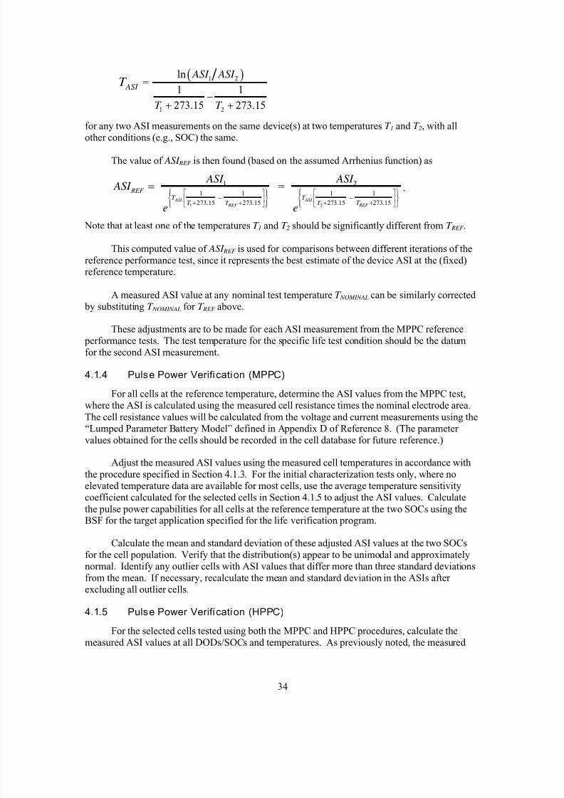
8/11/2019 Battery Life Verification Test Manual
http://slidepdf.com/reader/full/battery-life-verification-test-manual 46/133
34
( )1 2
1 2
ln
=1 1
273.15 273.15
ASI
ASI ASI
T T
T −
+ +
for any two ASI measurements on the same device(s) at two temperatures T 1 and T 2, with all
other conditions (e.g., SOC) the same.
The value of ASI REF is then found (based on the assumed Arrhenius function) as
1 2
1 2
1 1 1 1
273.15 273.15 273.15 273.15
ASI ASI
REF REF
REF T T
T T T T
ASI ASI ASI
e e
⎧ ⎫ ⎧ ⎫⎡ ⎤ ⎡ ⎤⎪ ⎪ ⎪ ⎪− −⎨ ⎬ ⎨ ⎬⎢ ⎥ ⎢ ⎥+ + + +⎪ ⎪ ⎪ ⎪⎣ ⎦ ⎣ ⎦⎩ ⎭ ⎩ ⎭
= = .
Note that at least one of the temperatures T 1 and T 2 should be significantly different from T REF .
This computed value of ASI REF is used for comparisons between different iterations of thereference performance test, since it represents the best estimate of the device ASI at the (fixed)reference temperature.
A measured ASI value at any nominal test temperature T NOMINAL can be similarly corrected by substituting T NOMINAL for T REF above.
These adjustments are to be made for each ASI measurement from the MPPC reference performance tests. The test temperature for the specific life test condition should be the datumfor the second ASI measurement.
4.1.4 Pulse Power Verification (MPPC)
For all cells at the reference temperature, determine the ASI values from the MPPC test,where the ASI is calculated using the measured cell resistance times the nominal electrode area.
The cell resistance values will be calculated from the voltage and current measurements using the“Lumped Parameter Battery Model” defined in Appendix D of Reference 8. (The parameter values obtained for the cells should be recorded in the cell database for future reference.)
Adjust the measured ASI values using the measured cell temperatures in accordance withthe procedure specified in Section 4.1.3. For the initial characterization tests only, where noelevated temperature data are available for most cells, use the average temperature sensitivitycoefficient calculated for the selected cells in Section 4.1.5 to adjust the ASI values. Calculatethe pulse power capabilities for all cells at the reference temperature at the two SOCs using theBSF for the target application specified for the life verification program.
Calculate the mean and standard deviation of these adjusted ASI values at the two SOCs
for the cell population. Verify that the distribution(s) appear to be unimodal and approximatelynormal. Identify any outlier cells with ASI values that differ more than three standard deviationsfrom the mean. If necessary, recalculate the mean and standard deviation in the ASIs after excluding all outlier cells.
4.1.5 Pulse Power Verification (HPPC)
For the selected cells tested using both the MPPC and HPPC procedures, calculate themeasured ASI values at all DODs/SOCs and temperatures. As previously noted, the measured
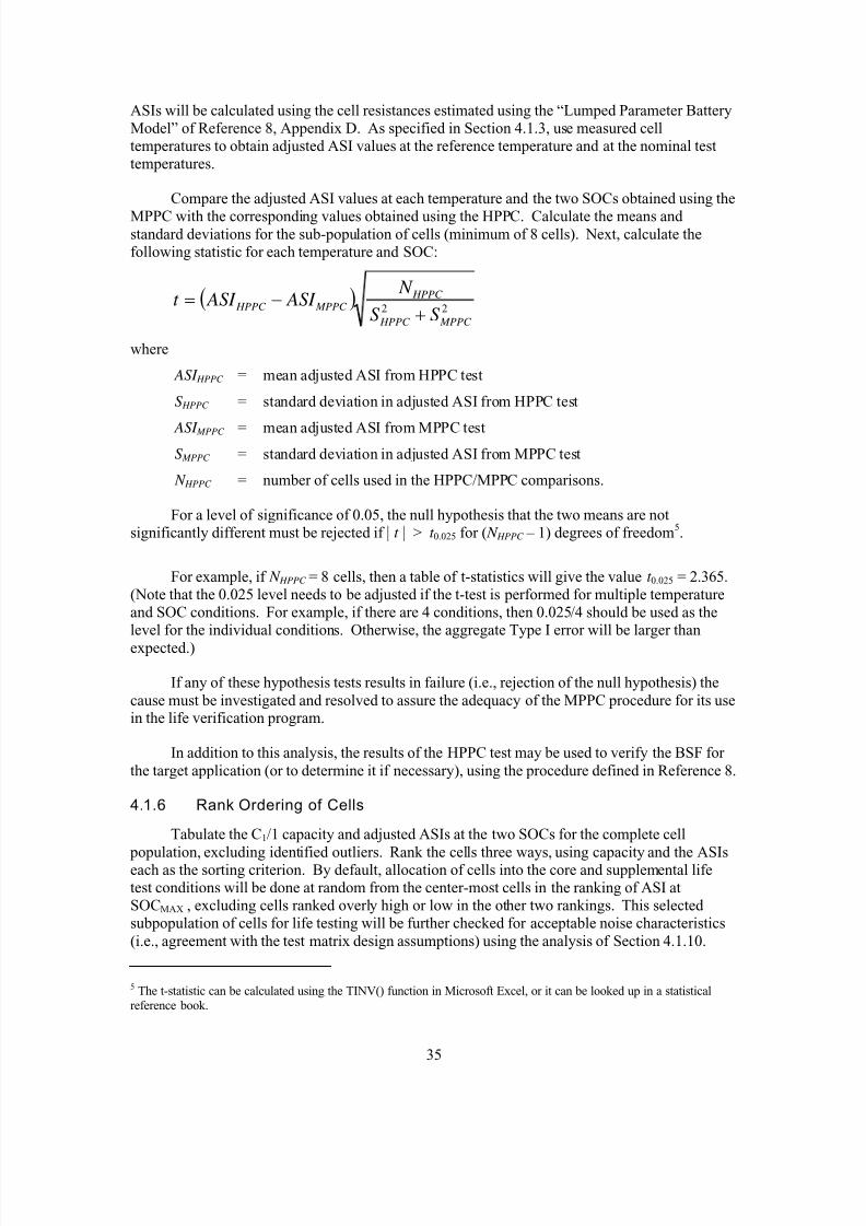
8/11/2019 Battery Life Verification Test Manual
http://slidepdf.com/reader/full/battery-life-verification-test-manual 47/133
35
ASIs will be calculated using the cell resistances estimated using the “Lumped Parameter BatteryModel” of Reference 8, Appendix D. As specified in Section 4.1.3, use measured celltemperatures to obtain adjusted ASI values at the reference temperature and at the nominal testtemperatures.
Compare the adjusted ASI values at each temperature and the two SOCs obtained using the
MPPC with the corresponding values obtained using the HPPC. Calculate the means and standard deviations for the sub-population of cells (minimum of 8 cells). Next, calculate thefollowing statistic for each temperature and SOC:
( )22
MPPC HPPC
HPPC MPPC HPPC
S S
N ASI ASI t
+−=
where
ASI HPPC = mean adjusted ASI from HPPC test
S HPPC = standard deviation in adjusted ASI from HPPC test
ASI MPPC = mean adjusted ASI from MPPC testS MPPC = standard deviation in adjusted ASI from MPPC test
N HPPC = number of cells used in the HPPC/MPPC comparisons.
For a level of significance of 0.05, the null hypothesis that the two means are notsignificantly different must be rejected if | t | > t 0.025 for ( N HPPC – 1) degrees of freedom5.
For example, if N HPPC = 8 cells, then a table of t-statistics will give the value t 0.025 = 2.365.(Note that the 0.025 level needs to be adjusted if the t-test is performed for multiple temperatureand SOC conditions. For example, if there are 4 conditions, then 0.025/4 should be used as thelevel for the individual conditions. Otherwise, the aggregate Type I error will be larger than
expected.)
If any of these hypothesis tests results in failure (i.e., rejection of the null hypothesis) thecause must be investigated and resolved to assure the adequacy of the MPPC procedure for its usein the life verification program.
In addition to this analysis, the results of the HPPC test may be used to verify the BSF for the target application (or to determine it if necessary), using the procedure defined in Reference 8.
4.1.6 Rank Ordering of Cells
Tabulate the C1/1 capacity and adjusted ASIs at the two SOCs for the complete cell
population, excluding identified outliers. Rank the cells three ways, using capacity and the ASIseach as the sorting criterion. By default, allocation of cells into the core and supplemental lifetest conditions will be done at random from the center-most cells in the ranking of ASI atSOCMAX , excluding cells ranked overly high or low in the other two rankings. This selected subpopulation of cells for life testing will be further checked for acceptable noise characteristics(i.e., agreement with the test matrix design assumptions) using the analysis of Section 4.1.10.
5 The t-statistic can be calculated using the TINV() function in Microsoft Excel, or it can be looked up in a statisticalreference book.
8/11/2019 Battery Life Verification Test Manual
http://slidepdf.com/reader/full/battery-life-verification-test-manual 48/133
36
4.1.7 Self-Discharge Rate Characterization
Calculate the average self-discharge rate (in Ah per day) for the cells tested at eachtemperature, using periodic measurements of OCV over the one-week test duration. The end-of-test OCV is used to estimate the final SOC (using the results of Section 4.1.1) and average lossrate, which are also confirmed by the residual discharge at the end of the test. These data may be
used to develop a correlation between self discharge and SOC (voltage) and to predict thefrequency of recharge needed to maintain the calendar life test cells within the specified minimum and maximum SOCs. Plot the estimated self-discharge rates versus test temperature for all cells tested to determine the level of consistency in these data. If necessary to obtain reliableestimates, repeat the self-discharge tests at selected temperatures using additional cells.
4.1.8 Cold-Cranking Power Verif ication
For each selected cell, calculate the pulse resistance and cold-cranking power capability at beginning of life for each of the three test pulses at the two SOCs using the method described inReference 8, Section 4.5. Also compute the estimated mean and standard deviation of theresistance and cold-cranking power for each of the pulses. (Ignore any data where voltagelimiting is encountered during a test pulse.) For each cell tested, plot the pulse resistance from
the first pulse versus the ASI at the reference temperature for each of the two SOCs to determinewhether outliers are present.
Recalculate the mean and standard deviation after excluding any outliers with first-pulseresistances that differ more than three standard deviations from the mean. If necessary, selectadditional cells from the population to conduct the cold-cranking test, such that the desired number of cells is obtained for this supplemental test condition.
Verify that the mean measured cold-cranking power capability meets or exceeds therequirement of the target application.
4.1.9 AC EIS Characterization
Examine the AC impedance spectra for anomalous characteristics, primarily in the form of cells whose behavior differs greatly from the average of the test population. This can be done bydetermining the equivalent series resistance (ESR) and/or the ionic impedance of each cell and
plotting these characteristics versus the ASI at the SOC value used for the EIS testing. (Someinformation on the interpretation of EIS results is found in Appendix C of Reference 11, and inReference 17.)
4.1.10 ASI Noise Characterization
The variation in ASI measurements for all cells from the initial characterization using theMPPC procedure will be analyzed using the following method. Each adjusted ASI measurementmay be seen as the “true” ASI value for the technology, plus a random effect due to cell-to-cell
manufacturing variation, plus an independent random error in the ASI measurement. Thatis: meascelltechmeas ASI ASI ε δ ++= . Without the measurement error, the true (but unobservable)
ASI value for a cell is given by celltechtrue ASI ASI δ += .
Three sources of variation are considered: cell-to-cell differences in electrode area, cell-to-cell differences in the (fixed) ohmic resistance, and measurement-to-measurement differences inthe ASI measurement error. The last of these sources is primarily due to random errors in the celltemperature measurement used to adjust the ASI measurement, plus random errors in the

8/11/2019 Battery Life Verification Test Manual
http://slidepdf.com/reader/full/battery-life-verification-test-manual 49/133
37
measured electrical parameters used to calculate ASI. The cell-to-cell effects are assumed to be perfectly reproducible, in the sense that they will be repeatable from measurement tomeasurement. The measurement variation is assumed to be perfectly uncorrelated, in the sensethat it is purely random, with zero mean and constant standard deviation.
The standard deviation of the measurement error (σ ε ) can be estimated by considering the
relationship between the ASI measurements from the same cell at two different SOC ’s, denoted by SOC MAX and SOC MIN . The assumed underlying relationship between the true ASI values of the
ith cell at the two different SOC’s is given by i
MAX true
i
MIN true ASI ASI )(10)( ⋅+= β β . The observed
ASI measurements are given by ( ) i
MIN meas
i
MIN true MIN
i
measi ASI SOC ASI Y )()( ε +== and
( ) i
MAX meas
i
MAX true MAX
i
measi ASI SOC ASI X )()( ε +== . Two procedures for estimating the model
parameters ( β 0 and β 1) are given here.
The first procedure, simple orthogonal regression, is recommended when there are noanomalous observations with unusually large deviations from the assumed linear relationship. Inthis case, the estimated model parameters are
( ) XY
XY XX YY XX YY
S
S S S S S
⋅⋅+−+−=
2
4ˆ22
1 β and
X Y ⋅−= 10ˆˆ β β ,
where
( )
( )11
2
−
−=
∑=
n
X X
S
n
i
i
XX ,
( )
( )11
2
−
−=
∑=
n
Y Y
S
n
i
i
YY ,
( ) ( )
( )11
−
−⋅−=
∑=
n
Y Y X X
S
n
i
ii
XY ,
n
X
X
n
i
i∑=
=1
, n
Y
Y
n
i
i∑=
=1
,
and n is the number of cells.
The second procedure uses robust orthogonal regression to estimate β 0 and β 1 (see section1.2 of Appendix B for details) with X i and Y i defined as above. This procedure is relativelyinsensitive to outliers and thus can be useful even when there are a few anomalous observations.
In either case of orthogonal regression (simple or robust), the orthogonal distance from the point ( X i, Y i) to the fitted line is given by
1ˆ
ˆˆ
21
10
+
⋅−−=
β
β β ii
i
X Y D .
When simple orthogonal regression is used, an estimate of ε σ is given by
( )11
2
−=
∑=
n
D
S
n
i
i
T MEASUREMEN .

8/11/2019 Battery Life Verification Test Manual
http://slidepdf.com/reader/full/battery-life-verification-test-manual 50/133
38
When robust orthogonal regression is used, a useful estimate of ε σ is given by
iT MEASUREMEN DmedianS ⋅= 48.1 . Estimates of the standard deviation of the variation in ASI
measurements (ASIMAX and ASIMIN) induced by manufacturing are given by
( ) 22
T MEASUREMEN MAX MAX MFG
S S S −= and
( ) 22T MEASUREMEN MIN MIN MFG S S S −= , where
S MEASUREMENT = estimated standard deviation of the measurement error
(S MFG) MAX = estimated standard deviation of the component of variation in theadjusted ASIs at SOCMAX induced by manufacturing
(S MFG) MIN = estimated standard deviation of the component of variation in theadjusted ASIs at SOCMIN induced by manufacturing
S MAX = standard deviation of the adjusted ASIs at SOCMAX
S MIN = standard deviation of the adjusted ASIs at SOCMIN
The two estimates for the standard deviation in the manufacturing variations are expected to be nearly equal.
Then, the values of ASI at maximum OCV will be plotted versus the inverse of the C1/1capacity to estimate the variations in ASI due to variation in electrode area. (Alternatively, in-
process data from the cell manufacturing operations may be used to assess the variation in ASIdue to variation in electrode area.) The balance of the variation is assumed to be due to cell-to-cell variation in the ohmic component of resistance. The result is as follows:
22
AREA MFGOHMIC S S S −= = estimated standard deviation in cell-to-cell ohmic ASI
where
( ) ( )2 2
2
MFG MFG MAX MIN MFG
S S S
+=
= rms estimated standard deviation in cell-to-cell manufacturing variation
( ) /1 at BOLC/1 capacity
C AREA Average ASI
Average
S S =
= estimated standard deviation in cell-to-cell electrode area variation
where S C/1 = standard deviation in C1/1 capacity.
These estimated values of S MEASUREMENT , S OHMIC , and S AREA are to be compared to the valuesused in the original experiment design to verify that the design will meet the TLVT programobjectives.
8/11/2019 Battery Life Verification Test Manual
http://slidepdf.com/reader/full/battery-life-verification-test-manual 51/133
39
4.2 Core Matrix Life Test Results
ASI test data for the core matrix of calendar life and cycle life test conditions will beanalyzed to estimate the mean and 90% lower confidence limit for the battery life in service at thespecified reference temperature and mix of cycling power levels. The preferred analysis method would be based on the calibrated life models for each specific candidate technology. Otherwise,
the empirical model presented in Appendix B will be used.
Regardless of which data analysis model is used, there are three main steps involved in projecting life in service from the test results. First, the ASI data are analyzed to estimate the life
on test (with the associated uncertainty) at each test condition in the matrix, ( ˆˆ andTEST TEST L
L S ).
A method called the “bootstrap” is suggested for estimating the uncertainty of the estimated life-on-test. Second, the lives-on-test for the calendar life test conditions, (P/P RATED = 0) are analyzed
to estimate the calendar life acceleration factor ( CALF ˆ ) using a weighted regression method. The
results are estimates for the mean and standard deviation of calendar life at the specified reference
temperature, ( CAL L and CALS ˆ ). Third, the lives on test for the cycle life test conditions are
correlated with the cycling stress factors and levels to estimate the contributions of the CYC F ˆfunction to the acceleration factors. Finally, the mean and 90% lower confidence limit for the
battery technology’s life in service are estimated for the FreedomCAR-specified combination of
cycle life requirements applied at the specified reference temperature, ( SERV SERV S L ˆand ˆ ).
The analysis methods used in this process are summarized in the following.
4.2.1 Life on Test Estimates
At each experimental condition, ASI data are analyzed to estimate the life on test (withassociated uncertainty). To illustrate, consider the default empirical data analysis model (see
Appendix A), ( ) ( )0 1 RPT ASI ASI t t t β β + ∆ = + ⋅ , where there are three model parameters: ASI 0, β ο , and β 1 . It is assumed that there are m observed values of ASI, 0 1 2, , , ,i i i im
ASI ASI ASI ASI … ,
for the ith of n cells on test. These values form the basis for the Robust Orthogonal Regression
(ROR) estimation procedure for ASI 0, β ο and β 1 (see Appendix B) given by 0 0 1ˆ ˆ ˆ, and ASI β β .
Using these parameter estimates, we estimate life-on-test as:
( ) ( )
( ) ( )[ ]
⎪⎭
⎪⎬⎫
⎪⎩
⎪⎨⎧
⋅−+−⎥⎥⎦
⎤
⎢⎢⎣
⎡⎟⎟ ⎠
⎞⎜⎜⎝
⎛
−⋅−+⋅
∆= 010
010
1
ˆ1ˆˆlog1
ˆ1ˆˆlog
ˆlogˆ I S A
PF
I S At L RPT
TEST β β β β β
where PF is the maximum allowable fraction of degradation.
To illustrate this process (normally applied to real test data), a single simulation wasconducted for each of the conditions described in Table 2.3-3 with the indicated number of cellsused for each condition. The noise levels used are as described in Section 2.3.1: (a) cell-to-cellfixed ohmic variation = 1%, (b) cell-to-cell electrode area variation = 0.5%, and (c) ASImeasurement error = 1%. The simulated ASI data were analyzed by ROR (see Appendix B) toobtain estimates of the model parameters. Using the parameter estimates, LTEST was estimated asdescribed above.

8/11/2019 Battery Life Verification Test Manual
http://slidepdf.com/reader/full/battery-life-verification-test-manual 52/133
40
The uncertainty of the various estimated model parameters and life on test can be assessed by using the bootstrap, which is a procedure for estimating the uncertainty associated withcomplex estimation procedures. The bootstrap is a well-established, well-accepted procedureused by many statisticians (e.g., see Reference 7). The motivation for using the bootstrap here isthe complex nature of the estimation procedure ROR for which it is difficult to analytically derivea useful estimate of the standard errors for the model parameters: ASI 0, β ο , and β 1 .
Table 4.2-1 summarizes the analysis of the simulated ASI data, including bootstrapstandard errors based on 100 bootstrap samples. The bootstrap standard error provides a notionof the uncertainty of each estimated quantity given a single set of experimental data as would bethe case in an actual experiment. Confidence intervals for LTEST should be derived directly from
percentiles of the empirical distributions of the bootstrap estimates of LTEST .
Table 4.2-1. Simulated experimental results: estimates compared with truth.(Bootstrap standard errors of estimates are in parentheses.)
Test Condition ASI 0 0 I S A 0 β 0
ˆ β 1 β 1
ˆ β LTEST TESTL
Calendar Life 1 30 29.98
(0.06)
1.092 1.04
(0.06)
0.974 0.975
(0.0019)
5.99 5.53
(0.46)Calendar Life 2 30 29.93
(0.11)1.456 1.43
(0.10)0.965 0.966
(0.0028)4.47 4.26
(0.77)
Calendar Life 3 30 29.90(0.17)
1.921 2.19(0.15)
0.954 0.946(0.0044)
3.37 3.76(0.93)
Calendar Life 4 30 30.04(0.24)
2.509 2.22(0.20)
0.939 0.947(0.0057)
2.56 2.49(0.24)
Cycle Life 1 30 30.01(0.08)
1.486 1.47(0.10)
0.964 0.965(0.0031)
4.38 4.53(0.63)
Cycle Life 2 30 30.18(0.16)
1.708 1.52(0.15)
0.959 0.965(0.0045)
3.80 3.20(0.32)
Cycle Life 3 30 29.65(0.23)
2.660 2.97(0.24)
0.936 0.927(0.0069)
2.41 2.51(0.82)
Cycle Life 4 30 29.89(0.20)
3.081 3.38(0.24)
0.926 0.918(0.0067)
2.07 1.96(0.19)
Figure 4.2-1 compares the cumulative distribution of the bootstrap results for the simulated ASI results in the Calendar Life 1 case in Table 4.2-1. It can be seen in Figure 4.2-1 that despitethe skewed distribution of the bootstrap values of life on test in this particular example, thenormal approximation of the distribution of bootstrap values (based on LTEST and the bootstrapstandard error) can still be used to obtain a useful lower 90% confidence limit for the life on test. 6
6 Because the distribution of TEST L is highly skewed, however, it may not be generally appropriate to derive
confidence limits for LTEST based on a normal approximation using the bootstrap standard error of TEST L .

8/11/2019 Battery Life Verification Test Manual
http://slidepdf.com/reader/full/battery-life-verification-test-manual 53/133
41
0
10
20
30
40
50
60
70
80
90
10 0
4.0 4.5 5.0 5.5 6.0 6.5 7.0 7.5 8.0 8.5
Li fe-on-Test (years )
C u m u l a t i v e D i s t r i b u t i o n
( % b
e l o w
i n d i c a t e d L i f e - o n - T e s t )
Normal Dist r ibut ion
Boo tst rap Resul ts (100 t r ials)
Figure 4.2-1. Comparison of bootstrap results with normal distribution for life on test atCalendar Life 1 test condition.
4.2.2 Calendar Life Estimate
The above results of Table 4.2-1 are used to estimate the calendar life and calendar lifeacceleration factors using the general equation for the calendar life test conditions:
I CALCAL I TEST F L L ,, = for I = 1.. N CAL
where I I I CAL I CAL SOC T F F ,,, = .
For the example life test matrix,7
,
1 1
273.15 273.15expCAL I ACT
REF I
F T T T + +
⎧ ⎫⎡ ⎤⎪ ⎪= −⎨ ⎬⎢ ⎥
⎪ ⎪⎣ ⎦⎩ ⎭
where
SOC I = SOC REF for I = 1.. N CAL (i.e. all calendar life testing is at the same SOC)
N CAL = 4 T I = 45, 50, 55, and 60ºC for I = 1..4.
In this case, the following weighted linear regression method can be used to estimate CAL L
and ACT T :
7 Note that the example life test matrix is based on the simple model of Section 2.1. Extension to additional stressfactors (e.g. SOC, throughput, P DIS and P RGN etc. is not performed in this manual.)
8/11/2019 Battery Life Verification Test Manual
http://slidepdf.com/reader/full/battery-life-verification-test-manual 54/133
42
( ) I I TEST I X LY β α +== ,ln
where1 1
273.15 273.15
I
REF I
X T T
= −+ +
, ACT CAL T L −== β α and )ln( .
The weights used in the linear regression are
2
,
,
ˆ
TEST
TEST I
I
L I
LW S
⎛ ⎞
= ⎜ ⎟⎜ ⎟⎝ ⎠
. The slope and intercept of the
linear regression model are then estimated by
( ) Y W diag D DW diag D B T T ⋅⋅⋅⋅⋅= −
)()(1
,
where D is a 4 × 2 matrix (first column is a vector of ones, second column contains the X i‘s), Y isa 4 × 1 vector containing the Y i‘s, and W is a diagonal matrix with the W I ‘s on the diagonal. The
first element of B is ˆ,α which estimates the intercept. The second element of B is ˆ, β which
estimates the slope.
Using the values for I TEST L ,
ˆ and
2
,TEST L I S from Table 4.2-1 in these equations gives theresults summarized in Table 4.2-2, based on the following derived values of the slope and intercept, respectively:
583.2ˆ =α
5575ˆ −= β .
These give the following results for the calendar life (at T REF = 30°C) and activationtemperature:
CAL L = expα ˆ = 13.23 years
versus the true value of LCAL = 15.22 yearsand
ACT T = β − = 5575 K
versus the true value of T ACT = 6000 K.
In addition to these results, Reference 6 provides a method for estimating the uncertainty in
α ˆ , which can be used to estimate the uncertainty in CAL L . For this example, the standard error of
α ˆ is 0.085. By error propagation (see Reference 20), an approximate standard error of CAL L is
1.1 years. Although this uncertainty is significantly larger than expected, it is due to the
relatively small number of test conditions (four) and the sensitivity of the life estimate to the parameter uncertainties for the example technology, with its low value of RATIO ASI
•
(0.125). In
such cases it may be desirable to use an alternative response variable, as discussed further inAppendix A.
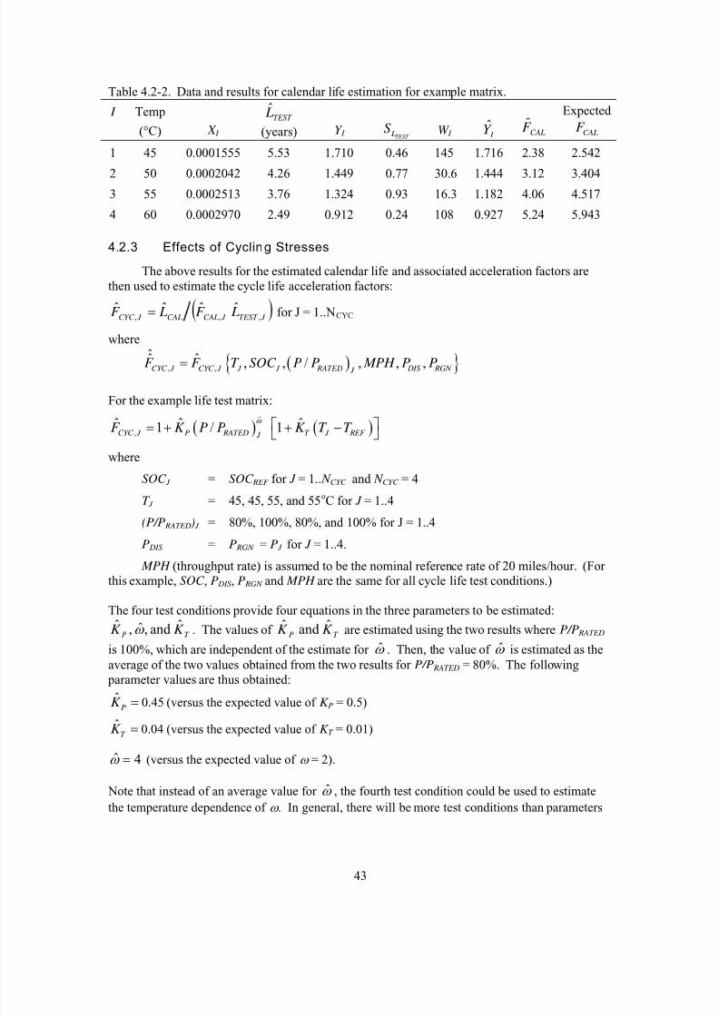
8/11/2019 Battery Life Verification Test Manual
http://slidepdf.com/reader/full/battery-life-verification-test-manual 55/133
43
Table 4.2-2. Data and results for calendar life estimation for example matrix.
I Temp
(°C) X I
TEST L
(years) Y I TEST LS W I I Y CALF ˆ
Expected
CALF
1 45 0.0001555 5.53 1.710 0.46 145 1.716 2.38 2.542
2 50 0.0002042 4.26 1.449 0.77 30.6 1.444 3.12 3.4043 55 0.0002513 3.76 1.324 0.93 16.3 1.182 4.06 4.517
4 60 0.0002970 2.49 0.912 0.24 108 0.927 5.24 5.943
4.2.3 Effects of Cycling Stresses
The above results for the estimated calendar life and associated acceleration factors arethen used to estimate the cycle life acceleration factors:
( ) J TEST J CALCAL J CYC LF LF ,,,ˆˆˆˆ = for J = 1..NCYC
where
( ) , ,ˆ ˆ , , / , , ,CYC J CYC J J J RATED DIS RGN J F F T SOC P P MPH P P=
For the example life test matrix:
( ) ( )ˆ
,ˆ ˆ ˆ1 / 1CYC J P RATED T J REF J F K P P K T T
ω ⎡ ⎤= + + −⎣ ⎦
where
SOC J = SOC REF for J = 1.. N CYC and N CYC = 4
T J = 45, 45, 55, and 55oC for J = 1..4
(P/P RATED) J = 80%, 100%, 80%, and 100% for J = 1..4
P DIS = P RGN = P J for J = 1..4.
MPH (throughput rate) is assumed to be the nominal reference rate of 20 miles/hour. (For this example, SOC , P DIS , P RGN and MPH are the same for all cycle life test conditions.)
The four test conditions provide four equations in the three parameters to be estimated:
T P K K ˆand ,ˆ,ˆ ω . The values of T P K K ˆand ˆ are estimated using the two results where P/P RATED
is 100%, which are independent of the estimate for ω . Then, the value of ω is estimated as theaverage of the two values obtained from the two results for P/P RATED = 80%. The following
parameter values are thus obtained:
0.45ˆPK = (versus the expected value of K P = 0.5)
0.04ˆT
K = (versus the expected value of K T = 0.01)
ˆ 4ω = (versus the expected value of ω = 2).
Note that instead of an average value for ω , the fourth test condition could be used to estimate
the temperature dependence of ω . In general, there will be more test conditions than parameters

8/11/2019 Battery Life Verification Test Manual
http://slidepdf.com/reader/full/battery-life-verification-test-manual 56/133
44
to be estimated from those conditions. The method of estimation to be used will depend on theexact nature of the assumed functional form of the cycle life acceleration factor.
The results for the values of CYC F ˆ are summarized in Table 4.2-3.
Table 4.2-3. Data and results for estimation of cycle life acceleration factors for example matrix.
J
Temp(°C) (P/PRATED)
TEST L CALF ˆ CYC F ˆ CYC F ˆ Expected
F CYC
1 45 80% 4.53 2.38 1.22 1.29 1.368
2 45 100% 3.20 2.38 1.73 1.72 1.575
3 55 80% 2.51 4.06 1.50 1.38 1.400
4 55 100% 1.96 4.06 1.92 1.90 1.625
4.2.4 Life in Service Estimate
The estimated life in service is found using the following general expression:
NOM CYC CALSERV F L L ,ˆˆˆ =
where
( )( ) ( ) ( ) ( ) ( )ˆ ˆ ˆ
,
0.8 0.6 0.15 0.8 0.05 0.951
15ˆ ˆCYC NOM P
F K
ω ω ω + +
+=
= 1.006
versus F CYC,NOM ≈ 1.014 for the numerical values of K P and ω from Section 2.1. The result is
SERV L = 13.1 years.
This estimate implies that there is a 50% chance that the actual life in service is greater than this value. Conversely, there is a 50% chance that the actual life in service is less than thisvalue. An interesting question is then, “How much less could it be?” One way to answer thisquestion is to estimate the 90% lower confidence limit for the life in service. There is a 90%chance that the actual life-in-service will be greater than this limit.
In the present example, the life in service is primarily determined by the calendar life, due
to the value of NOM CYC F ,ˆ being nearly unity. A reasonable approximation is then:
CALSERV S S ˆˆ ≈
so that the estimate for the 90% lower confidence limit of life in service is approximately
( ) ( ),90% 0.1 1 7ˆˆ ,ˆSERV CAL ST TC SERV LCL L S t p N L ν =− = = −= = 11.6 years
where
t pST , ν = value of t-statistic for ν degrees of freedom and pST single-tailed probability
= 1.415 for the example life test matrix.

8/11/2019 Battery Life Verification Test Manual
http://slidepdf.com/reader/full/battery-life-verification-test-manual 57/133
45
4.3 Supplemental Life Test Resul ts
In all cases except for the HPPC life test cells noted in Section 2.4, the supplemental lifetest data are used to test hypotheses based on differences in the measured ASI data betweensamples from different groups of cells. The general procedure for this statistical analysis is
summarized below, followed by summaries of how this procedure would be applied in the threecandidate supplemental life tests.
4.3.1 Hypothesis Testing
Hypothesis testing associated with the supplemental life test matrix may be done using thegeneral t-statistic, based on small samples, for the difference between two means:
( ) ( )
( )
21
2121
222
211
21 2
11 nn
nnnn
S nS n
X X t
+
−+⋅⋅⋅
⋅−+⋅−
−=
where21, X X = estimated means for a parameter for each of two groups of cells (e.g. ASI)
S 1, S 2 = standard deviations of the data for each of the two groups
n1, n2 = number of cells for each of the two groups.
The hypothesis to be tested is that there is no underlying difference in mean performance between
the two groups. That is 21 = , where µ 1 and µ 2 are the population averages associated with
the two groups that are sampled. 1 X and 2 X are sample estimates of µ 1 and µ 2 .
There are three possible corresponding alternate hypotheses:
(1) 021 <− (2) 021 >− (3) 021 ≠−
The first two are one-sided alternates; the last alternate is two-sided.
A level of significance, α, must be specified before the test. For the purposes of thismanual, a value of 0.05 is suggested for α. Then, the corresponding criteria for rejection of thenull hypothesis in favor of one of the alternate hypotheses are:
(1) t < – T α (2) t > T α (3) | t | > T α /2
Values of T α and T α /2 are available from standard tables for the t-distribution with varyingdegrees of freedom, ν . In general, for these tests ν = n1 + n2 – 2.
4.3.2 Combined Calendar/Cycle Life tests
There are four groups of cells that must be analyzed to assess the path-independence of theASI growth. Two groups are from the core matrix, both at the same test temperature, but withone group in the calendar life submatrix and the second group in the cycle life submatrix. Thecorresponding two groups in the supplemental life test matrix use the same test conditions as thecore matrix groups, but with a switchover from one test condition to the other at a specified valueof ASI.

8/11/2019 Battery Life Verification Test Manual
http://slidepdf.com/reader/full/battery-life-verification-test-manual 58/133
46
An example of the expected ASI time histories for the two supplemental matrix groups isshown in Figure 4.3-1. These histories are based on the expected performance for thecorresponding core matrix test conditions for the example minimum experiment design presented in Section 2. The dashed histories show the expected ASI growth for the core matrix conditions,while the solid histories show the expected ASI growth for the supplemental matrix conditionswith the switchover from one condition to the other occurring at a prespecified ASI of 34.7 Ω-
cm2. It is apparent that the ASI rates of change for the two supplemental groups of cells areshifted at the switchover point. The two hypotheses to be considered are whether the shifted ASIrates of change are equal to the rates of change of the corresponding groups in the core matrix atthe same ASI values.
28
30
32
34
36
38
40
42
0 8 16 24 32 40 48 56 64 72 80 88 96 104
Weeks on Test
A S I ( - c m
2
)
ASI at tr ansition = 34.7
Calendar/Cycle
Cycle/Calendar
T=55oC (P/PRATED) = 0 and 100%
Figure 4.3-1. Expected ASI histories for combined cycle/calendar and calendar/cycle testconditions.
Define the four groups of cells as follows:
Core1 = group of m1 calendar life cells in the core matrix at the specified temperatureCore2 = group of m2 cycle life cells in the core matrix at the specified temperatureCombined 1 = group of n1 cycle/calendar life cells in the combined matrix at the specified
temperature
Combined 2 = group of n2 calendar/cycle life cells in the combined matrix at the specified temperature
The four groups are analyzed to estimate the average ASI rates of change from the
switchover ASI value to the end of the test . Due to noise in the ASI data, there will be uncertaintyin the estimated rates of change. The test statistics to be used are:

8/11/2019 Battery Life Verification Test Manual
http://slidepdf.com/reader/full/battery-life-verification-test-manual 59/133
47
( ) ( )
( )
ii
iiii
iiii
iii
nm
nmnm
S n Rm
X Y t
+
−+⋅⋅⋅
⋅−+⋅−
−=
2
11 22, for i =1, 2,
where
iY = average ASI rate of change associated with the ith Combined group of
cells
S i = standard deviation of ASI rate of change associated with the ith
Combined group of cells
i X = average ASI rate of change associated with the ith Core group of cells
Ri = standard deviation of ASI rate of change associated with the ith Core
group of cells
In general, these statistics are used to assess whether or not the future ASI rate of change, beginning at a fixed/elevated ASI level, depends on how a cell has been previously been degraded
to that fixed ASI level. The first t-statistic (t 1) is used to assess whether or not the rate of calendar life degradation is affected unexpectedly by previous exposure to cycle life aging. The second t-statistic (t 2) is used to assess whether or not the rate of cycle life degradation is affected unexpectedly by previous exposure to calendar life aging.
For example, if |t 1| > T 0.025 with (m1 + n1 – 2) degrees of freedom, we conclude thatfuture calendar life aging (measured by the ASI level) depends on not just the current ASI leveland future calendar life stresses, but also the nature of the previous aging (calendar life versus
cycle life). Alternately, if 025.01 T t < , then one would not reject the hypothesis that future
calendar life aging depends only on the current ASI level and future calendar life stresses. If both
025.01 T t < and 025.02 T t < , then one would not have evidence to reject the hypothesis that future
cell aging depends only on the current ASI level and future stresses (i.e. path independence).
4.3.3 Cold-start Verifi cation Tests
To verify that cold starts do not significantly affect battery life, the estimated lives on testfor two of the core life test conditions will be compared with those for two supplemental groupsof cells tested under the same conditions, but with the addition of a cold start test conducted as part of every periodic reference performance test. See Section 4.2.1 for details on estimating thelife on test of cells under a specific condition. Here, the underlying hypothesis is that
( ) ( )CORE TEST START COLDTEST L L =− .
The alternate hypothesis is that:
( ) ( )CORE TEST START COLDTEST L L <− .
Rather than using a t-statistic, we use a standardized normal Z-statistic for each of the two
comparisons. The Z-statistics will be based on the estimated mean lives on test ( START COLD X −
and CORE X ) and the corresponding bootstrap standard errors of the estimates (S COLD-START and

8/11/2019 Battery Life Verification Test Manual
http://slidepdf.com/reader/full/battery-life-verification-test-manual 60/133
48
S CORE ). That is: ⋅⋅+
−=
−
−−
22CORE START COLD
CORE START COLDSTART COLD
S S
X X Z The criterion for rejecting the null
hypothesis is then: 65.1−<−START COLD Z
4.3.4 Low-temperature Operation Tests
For the supplemental life tests involving low-temperature operation, it may be impossibleto reliably estimate life on test due to limited cell degradation. Hence, it would be inappropriate to base a statistical test on such estimates. Instead, the average ASI rates of change over the full testduration will be used to evaluate the test statistic. Even then, the uncertainties in these rates will be relatively high, since there will be little ASI change if the tests are successful. Two groups of cells are considered. The first group (T=LIMIT ) represents very low temperature operation. In thesecond group (T>LIMIT ), the operating temperature is still low but close enough to standard testconditions so as to expect no significant ASI growth. If the first group of cells operating at thelimits of the performance constraints (T=LIMIT ) exhibit any significant ASI growth, it should be possible to differentiate the performance of the two groups and hence identify a degrading lowtemperature effect. The statistical test described in Section 4.3.1 will be used to determine if low-temperature operation affects battery life, without necessarily quantifying the magnitude of the
effect from these test results. Here, the underlying hypothesis is that the rate of ASI change over
the two conditions is the same: LIMIT T LIMIT T I S A I S A >= = .
The alternate hypothesis is that T LIMIT T LIMIT ASI ASI • •
= >> . The statistic to be used in this
case is
( ) ( )
( )
21
2121
22
21
2
11 nn
nnnn
S nS n
X X t
LIMIT T LIMIT T
LIMIT T LIMIT T TEMP LOW +
−+⋅⋅⋅
⋅−+⋅−
−=
=>
=>− , where
LIMIT T X > and LIMIT T X = denote the observed average ASI change for the two groups consisting of
n1 and n2 cells, respectively. LIMIT T S > and LIMIT T S = denote the standard deviation of the ASI
change for the two groups. In the case of 8 cells per group, the criterion for rejecting the nullhypothesis is 05.0t t TEMP LOW >− (14 degrees of freedom).

8/11/2019 Battery Life Verification Test Manual
http://slidepdf.com/reader/full/battery-life-verification-test-manual 61/133
49
5. REFERENCES
1. Advanced Technology Development Li-Ion Failure Modes Analysis (report in preparation).
2. Advanced Technology Development Program for Lithium-Ion Batteries: Gen 2 Performance
Evaluation Interim Report , INEEL/EXT-03-00095, February 2003.
3. Advanced Technology Development Program for Lithium-Ion Batteries: Handbook of Diagnostic Techniques, LBID-2464, April 2003.
4. Ammann, L. and Van Ness, J., “A Routine for Converting Regression Algorithms intoCorresponding Orthogonal Regression Algorithms,” ACM Transactions on Mathematical
Software, 14, 1988, pp. 76–87.
5. Box, G.E.P., Hunter, W. G., and Hunter, S. J., Statistics for Experimenters, New York: JohnWiley & Sons, 1978.
6. Draper, N. R. and Smith H., Applied Regression Analysis, 3rd edition, New York: JohnWiley & Sons, 1998.
7. Efron, B., and Tibshirani, R. J., An Introduction to the Bootstrap, New York: Chapman and
Hall, 1993.
8. FreedomCAR Battery Test Manual for Power-Assist Hybrid Electric Vehicles, DOE/ID-11069, 2003.
9. FreedomCAR 42-volt Battery Test Manual, DOE/ID-11070, 2003.
10. FreedomCAR Battery Test Manual for Fuel Cell Powered Vehicles (to be published).
11. FreedomCAR Ultracapacitor Test Manual, DOE/NE-ID-11173, September 2004.
12. Haskins, H. J., 2003, private communication, October 24, 2003.
13. Haskins, H. J., Development of Power Profiles for Hybrid Electric Vehicle Battery
Cycle life Testing (report in preparation).
14. Hedayat, A. S., Sloane, N. J. A., and Stufken, J., Orthogonal Arrays: Theory and
Applications, New York: Springer-Verlag, 1999.
15. Holland, P. and Welsch, R., “Robust Regression Using Iteratively Reweighted LeastSquares,” Communications in Statistics, Part A – Theory and Methods, 6, 1977, pp. 813–828.
16. Iglewicz, B., “Robust Scale Estimators and Confidence Intervals for Location,”Understanding Robust and Exploratory Data Analysis, D. C. Hoaglin, F. Mosteller, and J. W.Tukey, eds., New York: Wiley, p. 417, 1983.
17. Linden, David and Reddy, T. B., eds., Handbook of Batteries, third edition, New York:McGraw-Hill, 2002.
18. Meeker, W. Q. and Escobar, L. A., Statistical Methods for Reliability Data, Chapter 21,
“Accelerated Degradation Tests,” 1998, John Wiley and Sons, Inc.
19. PNGV Battery Test Manual, DOE/ID-10597, 2001.
20. Sveshnikov, A. A., Problems in Probability Theory, Mathematical Statistics and Theory of
Random Functions, W. B. Saunders, 1968.
21. Thomas, E. V., Case, H. L., Doughty, D. H., Jungst, R. G., Nagasubramanian, G. and Roth,E. P., “Accelerated Power Degradation of Li-Ion Cells”, Journal of Power Sources, 124,2003, pp. 254-260.

8/11/2019 Battery Life Verification Test Manual
http://slidepdf.com/reader/full/battery-life-verification-test-manual 62/133
50
22. Uncertainty Study of INEEL EST Laboratory Battery Testing Systems, INEEL/EXT-01-00505, Vol. 1, December 2001, and Vol. 2, March 2003.
8/11/2019 Battery Life Verification Test Manual
http://slidepdf.com/reader/full/battery-life-verification-test-manual 63/133
A-1
Appendix A
Life Test Simulation Programs

8/11/2019 Battery Life Verification Test Manual
http://slidepdf.com/reader/full/battery-life-verification-test-manual 64/133
A-2

8/11/2019 Battery Life Verification Test Manual
http://slidepdf.com/reader/full/battery-life-verification-test-manual 65/133
A-3
Appendix A
Life Test Simulation Programs
A-1. INTRODUCTION
Two Excel spreadsheet programs have been developed to support planning of battery technologylife verification testing. The primary objectives of these programs are to (1) optimize allocation of cellsto each test condition in the core life test matrix; and (2) estimate the 90% lower confidence limit for lifein service as a function of the total number of cells tested for candidate matrix designs. Evaluations of such matrix design variables as the number and level of stress factors, the test duration, and reference performance test intervals are facilitated for specified levels of manufacturing and test measurementvariation. A secondary objective of the two programs is final verification of the matrix design, given realtest data from initial characterization of the actual test cell population.
The first program is an Excel spreadsheet routine called Cell Allocator . It is used in the preliminary stage of the overall life test experiment design to provide initial allocation of cells to the test
conditions of the core life test matrix. It uses analytical approximations for the propagation of “noise” inthe area-specific impedance (ASI) measurements to determine uncertainties in the expected values of lifeon test at each matrix condition. The approximations are based on the expected, i.e., “true,” lifecapabilities of the candidate technology.
The second program, Battery MCS , is a Visual Basic Application spreadsheet for Monte Carlosimulation (MCS) and analysis of test data from one given test condition at a time. This routine also runsin the Excel environment and can automatically replicate the simulation of the test results for any givennumber of cells and any specified number of MCS trials. It is used to confirm the results of the preliminary experiment design generated using Cell Allocator . It also may be used to analyze either simulated or real test data for estimating the life on test for a given test condition, as well as estimatingthe uncertainty in that estimate.
The general approach used in the Battery MCS program assumes the particular methods of Appendix B for analysis of life test data. As noted in that appendix, the baseline, or default, analysismethod is empirical, with flexibility to accommodate a wide range of performance degradation behaviors.However, substitution of a physics-based model appropriate to the specific candidate technology isstrongly encouraged and is supported by the simulation program. The general simulation approachdocumented herein will then serve as a guide for customization of the programs by each developer.
The Monte Carlo method of simulation, as used in these programs, starts with a “truth” function for ASI, the parameter used to characterize battery performance degradation. Growth in ASI over timeresults in reduction in battery pulse power capability. Battery design guidelines established byFreedomCAR allow an initial margin of only 30% in pulse power capability, relative to the specified end of life performance goals. Thus, a power fade of 23% relative to power at beginning of life defines the
battery’s end of life.a The acceleration factor (AF) at each test condition is input to the simulation,defining the expected life on test at that condition.
The ASI truth function is corrupted by three sources of “noise” applied as additive or multiplicativerandom variables to simulate actual ASI measurements over time. The simulation program applies the
a Note that both programs default to an arbitrary value of 25% power fade for EOL. The user should change this to theappropriate program-specific value.

8/11/2019 Battery Life Verification Test Manual
http://slidepdf.com/reader/full/battery-life-verification-test-manual 66/133
A-4
same data analysis model that was used for the ASI truth function to these simulated test data. The dataanalysis results are estimates of the model parameters for the particular simulated data set. Theseestimated model parameters will differ from the true model parameters due to the noise added to the ASItruth function. In general, the level of uncertainty of the model parameters will reflect the magnitudes of the specified noise levels. The estimated model parameters are used to estimate life on test for the particular test condition. Uncertainty in the estimated life on test is also estimated as part of the data
analysis procedure. As described in Appendix B, this is based on a standard statistical procedure called the “bootstrap” method.
Results for the complete core matrix of test conditions can be combined to obtain an estimate of themean life in service at the conditions of normal usage. Further, the estimated uncertainties in the lives ontest can be used to provide a 90% lower confidence limit for the mean life in service. This final step hasnot been built into the simulation tool, due to the wide variety of possible stress factors and levels for anyspecific technology.
This appendix is organized into the following major sections. Section A-2 documents theequations used in the Battery MCS program, although the details of the test data analysis method aredocumented in Appendix B. Section A-3 documents the equations used in the Cell Allocator program.
Section A-4 describes an example life test experiment design.
A-2. SIMULATION EQUATIONS
The equations used in the Cell Allocator and Battery MCS programs are documented in thefollowing. First, the ASI truth function is described. Second, generating simulated ASI data using threespecified noise parameters is described. Third, the baseline empirical data analysis model is brieflysummarized. Finally, an alternative approach for estimating life on test is provided for use withtechnologies that may have self-limiting degradation mechanisms.
A-2.1 ASI Truth Funct ion
The ASI truth model is based on the following empirical model of test data, originally developed toanalyze the results of cell life testing conducted on Gen 2 cells in the DOE Advanced TechnologyDevelopment program. (See Appendix B for details.) The empirical model equation is:
ASIt t ASIt 1o RPT β β ˆˆ +=∆+
where
ASIt = measured area-specific impedance (Ω-cm2) at time t (weeks)
∆t RPT = interval (weeks) between reference performance test (RPT) measurements of ASI
o β and 1 β = estimates of the intercept and slope, respectively, of the linear relationship
between ASIt+ ∆t RPT and ASIt.
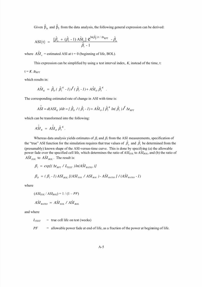
8/11/2019 Battery Life Verification Test Manual
http://slidepdf.com/reader/full/battery-life-verification-test-manual 67/133
A-5
Given oβ and 1β from the data analysis, the following general expression can be derived:
RPT
o 1 o o
1
ˆln( ) t / t1ˆ ˆ ˆ ˆ[ ( - 1) ASI ] -ASIt
ˆ - 1
e β β β β
β
∆+
=
where o I S A ˆ = estimated ASI at t = 0 (beginning of life, BOL).
This expression can be simplified by using a test interval index, K , instead of the time, t:
t = K ∆t RPT
which results in:
I S A1)-(1)-( I S AK
1O1
K
1OK / β β β β ˆˆˆˆˆˆ += .
The corresponding estimated rate of change in ASI with time is:
RPT 1
K
1O1OK t )ln(] I S A1)-( / [)/dt d(ASI I S A / ∆+== β β β β ˆˆˆˆˆ
which can be transformed into the following:
K
1OK I S A I S A β ˆˆ = .
Whereas data analysis yields estimates of β o and β 1 from the ASI measurements, specification of
the “true” ASI function for the simulation requires that true values of oˆ β and 1
ˆ β be determined from the
(presumably) known shape of the ASI-versus-time curve. This is done by specifying (a) the allowable power fade over the specified cell life, which determines the ratio of ASI EOL to ASI BOL, and (b) the ratio of
EOL I S A to BOL I S A . The result is:
)] I S ln(A) L / t exp[( RATIOTEST RPT 1∆= β
1)- I S (A / ] I S A-) ASI / [(ASI ASI 1)-( RATIO RATIO BOL EOL BOL1O β β =
where
( ASI EOL / ASI BOL) = 1 / (1 – PF )
BOL EOL RATIO I S A / I S A I S A =
and where
LTEST = true cell life on test (weeks)
PF = allowable power fade at end of life, as a fraction of the power at beginning of life.

8/11/2019 Battery Life Verification Test Manual
http://slidepdf.com/reader/full/battery-life-verification-test-manual 68/133
A-6
The true life on test is given by the target cell life in service of 15 years, divided by a calendar lifede-rating factor, and then divided by an acceleration factor ( AF ) associated with the specific actual testconditions:
LTEST = LCAL / AF
where
LCAL = true cell calendar life = LSERVICE / ( LCAL de-rating factor)
where LSERVICE = true life-in-service, including cycling effects at the nominal conditions of usage.
The conditions are that (a) ambient temperature is equal to reference temperature and (b) no batterycycling corresponds to AF = 1. The calendar life de-rating factor accounts for the effect on battery life of cycling at the nominal conditions of usage specified by FreedomCAR.
The shape of the ASI versus time curve is related to RATIO ASI •
as follows:
Increasing ASI rate of change ⇒ I S A RATIO > 1 ⇒ β1 > 1
Decreasing ASI rate of change ⇒ I S A RATIO < 1 ⇒ βO > 0 and β1 < 1 .
The special case for constant ASI rate over life implies I S A RATIO = 1, which then implies:
β 1 = 1
β O = ASI BOL [(ASI EOL / ASI BOL) - 1] (∆t RPT /LTEST ) > 0
ASIt = ASI O + β O t / ∆t RPT
= ASI O + ASI BOL [(ASI EOL / ASI BOL) - 1] t /LTEST .
Thus, a wide range of ASI shapes can be selected as the “true” ASI function in the simulation.Representative examples of such functions are illustrated in Figure 2.1-1 in the manual.
Note that the true ASI rate of change is given by:
RPT 1
K
1O1O t / )ln()(] ASI )1-( / [ I S A ∆+= β β β β
= β O / ∆t RPT for the special case of I S A RATIO = 1.
A-2.2 ASI Simulated Test Data Generation
In the simulation, the true ASI is “corrupted” by random cell-to-cell variations in ASI due tomanufacturing and by random errors in each ASI measurement over time. The simulated ASImeasurements are combinations of truth and three random variables:
Measured ASI = (F AREA) (ASI TRUE ) + ∆ ASI FIXED + ∆ ASI MEASUREMENT

8/11/2019 Battery Life Verification Test Manual
http://slidepdf.com/reader/full/battery-life-verification-test-manual 69/133
A-7
where
ASITRUE = [βO + (β1 – 1) ASIO ] exp[ln(β1) t / ∆tRPT] − βO / (β1 – 1)
= βO [(β1)K – 1] / ( β1 – 1 ) + ASIO (β1)
K
FAREA = (1 – ∆AELECT/AELECT ) = electrode area factor
∆AELECT / AELECT = cell-to-cell variation in electrode area / nominal electrode area
∆ASIFIXED = cell-to-cell variation in ASI due to fixed ohmic resistance variations
∆ASIMEASUREMENT = measurement-to-measurement ASI variation due to test equipment.
The three random variables are normally distributed with zero means and with input standard
deviations of σ AREA, σ FIXED, and σ MEASUREMENT , respectively. Specific values of ∆ A ELECT /A ELECT and
∆ ASI FIXED are generated for each cell using the program’s built-in random number generator to obtain thecell’s initial ASI at time = 0. Then, for each cell at each measurement time, the random number generator
is used to obtain independent values of ∆ ASI MEASUREMENT to be added to the cells’ ASI. The true growth in
each cell’s ASI includes the effect of electrode area variation, but not ∆ ASI FIXED, which remains constantover the cell’s life on test.
A-2.3 Test Data Analysis Model
Once the set of ASI measurements has been established, either by the simulation or from actual
testing, the data analysis method of Appendix B is used to estimate three model parameters: ˆO
β ,1
ˆ β , and
OˆASI . This is done using the following sequence.
The parameters ˆO
β and1
ˆ β are calculated using a robust orthogonal regression (ROR) method
developed to analyze data for which errors in the X-values are comparable to errors in the Y-values. Inthe ROR method, the data are given nonuniform weights to reduce the effects of outliers and data at the
extremes of the range in X-values.
The parameter I S A Oˆ is estimated by setting the average residual error (i.e., estimated ASI minus
measured ASI) to zero for the ASI data set.
The estimated life on test is calculated using the following equation:
( )1O1o
O1o
RPT TEST ln I S A1]-[
PF)-(1 / I S A1]-[t L
β β β
β β
ˆ
1
ˆˆˆ
ˆˆˆlnˆ
⎪⎭
⎪⎬⎫
⎪⎩
⎪⎨⎧
×+
+∆= .
Uncertainties inO
ˆ β , ˆ
1
β , ˆ ,O ASI and LTEST
ˆ are estimated using the bootstrap method, wherein the
residual errors in the parameters are resampled many times (≈100) to create alternate realizations of thetest data. These alternate data sets are each analyzed to get corresponding alternate values for the four
parameters. The standard errors in the parameters can then be estimated from the ≈100-sampledistributions obtained. This method has become a standard approach for this kind of analysis, and it has broad applicability beyond its use in the Battery MCS program.
Finally, the estimated lives on test and their associated uncertainties are used to estimate thecalendar life and life in service in an iterative procedure:

8/11/2019 Battery Life Verification Test Manual
http://slidepdf.com/reader/full/battery-life-verification-test-manual 70/133
A-8
1. The calendar life is initially estimated using a weighted regression of the lives on test versus theexpected acceleration factors for the several test conditions of the matrix. The calendar lifecorresponds to AF = 1 in the regression.
2. The acceleration factors are recalculated using the estimated calendar life and the estimated lives-on-test.
3. The calendar life is re-estimated using the recalculated acceleration factors.
4. Steps 2 and 3 are repeated until the calendar life estimate converges to a final estimate.
5. The life in service is estimated from the calendar life estimate and the estimated accelerationfactors for the cycle life test conditions of the matrix, adjusted for the pulse profiles specified byFreedomCAR for battery cycle life.
6. The 90% lower confidence limit for life in service is calculated approximately as:
LCL90,SERVICE ≈ LCAL – tα=0.1; ν=NTC – 1 SCAL
where
tα = 0.1; ν = NTC – 1 = the αth percentile of the t-distribution with ν degrees of freedom
NTC = number of test conditions in the core life test matrix
SCAL = standard error in the estimated calendar life, calculated using the estimated standard errors in the lives on test (see Appendix B).
A-2.4 Al ternative Equation for Life Est imation
For technologies that have self-limiting degradation mechanisms ( β 1 < 1), the estimated life on testcan become strongly dependent on the specified allowable power fade. This is because eventually, inthese cases, the ASI growth rate goes to zero. The limit value of ASI as time goes to infinity is:
( )10 1 β β −≡∞ ASI
( )
⎭⎬⎫
⎩⎨⎧
−
−−∆=⇒
∞
∞
0
0
1
1ln
ln ASI ASI
PF ASI ASI t L RPT
TEST β
where the condition ( )PF ASI ASI ASI EOL −=>∞ 10 is needed to obtain a finite estimate of LTEST .
The effect of the allowable power fade on estimated life is illustrated in Figure A-1 for the example
case of RATIO ASI •
= 0.125. Note that when noisy data are used to estimate the β O and β 1 parameters, it is
possible that the corresponding life estimates may become infinite, even when the mean value of ASI ∞
satisfies the above criterion. It may then be necessary to use the statistical distribution of ASI ∞ to estimate
the uncertainties in the estimated lives on test.

8/11/2019 Battery Life Verification Test Manual
http://slidepdf.com/reader/full/battery-life-verification-test-manual 71/133
A-9
0
5
10
15
20
25
30
0% 5% 10% 15% 20% 25%
Allo wab le Power Fade
L i f e - i n - S e r v i c e ( y e
a r s )
ASI' Ratio = 0.125
Figure A-1. Effect of allowable power fade on life in service for technologies with self-limitingdegradation mechanisms.
A-3. CELL ALLOCATOR PROGRAM
The Cell Allocator program provides an approximately optimum allocation of a given total number of test cells to the specified test conditions of the core life test matrix. The criterion used is that thestandard error in the estimated calendar life be minimized, given the estimated standard errors in the liveson test. The Battery MCS program can also be used to determine this optimum allocation, but CellAllocator is used to narrow the range of options in the preliminary experiment design stage. Then, theBattery MCS program can be used more effectively to confirm the preliminary design. The principaldifference in the two programs is that Cell Allocator uses approximate analytical expressions for the propagation of noise in the ASI data into the uncertainties in the lives on test. The Battery MCS programuses the empirical data analysis procedure, including the bootstrap method, to do the same thing morerealistically.
The approximate analytical expressions used in Cell Allocator are presented in the following. Theyare based on the total derivative of the estimated life on test with respect to the ASI data, evaluated assuming the “true” values of the parameters. It is first assumed that there is only one cell at each testcondition, and the standard error in the estimated life on test will vary inversely as the square root of thenumber of cells allocated to any given test condition.
The estimated life on test at each test condition is expressed in terms of the estimated model
parameters:
( ) ( )
( ) 11
1
ˆln
1
ˆ1ˆˆ
1/ˆ1ˆˆlnˆ
β β β
β β
⎪⎭
⎪⎬⎫
⎪⎩
⎪⎨⎧
−+
−−+⎟⎟ ⎠
⎞⎜⎜⎝
⎛ =
OO
OO
RPT
EOT TEST
I S A
PF I S A
N
t L .

8/11/2019 Battery Life Verification Test Manual
http://slidepdf.com/reader/full/battery-life-verification-test-manual 72/133
A-10
The approximate standard error in this estimate is, for only one cell on test:
( )
1/ 22
22 '
,1
,
ˆ
K
RPT
TEST LOT k ASI
k O N K
dLS ASI S
dASI =
⎡ ⎤⎛ ⎞⎢ ⎥= ⎜ ⎟⎜ ⎟⎢ ⎥⎝ ⎠⎣ ⎦
∑
where the total variance in the ASI data is
( ) ( ) ( ) ( )2'2'2'
2
,2'T MEASUREMEN FIXED AREA
O
TRUE K
ASI S S S ASI
ASI S
K ++⎟⎟
⎠
⎞⎜⎜⎝
⎛ = .
The total derivative of the estimated life on test with respect to each ASI measurement is calculated using the chain rule of differentiation:
1
1
ˆ ˆˆˆ ˆ ˆ ˆ
ˆ ˆ ˆTEST TEST TEST O TEST O
K K K K O O
dL L L L dASI
dASI ASI ASI dASI ASI
β β
β β
∂ ∂ ∂ ∂∂= ⋅ + ⋅ + ⋅
∂ ∂∂ ∂ ∂ .
The results for the three partial derivatives of life on test with respect to the model parameters areas follows:
( ) ( ) ( ) ⎟⎟ ⎠
⎞⎜⎜⎝
⎛ −
⎥⎥⎦
⎤
⎢⎢⎣
⎡
−+−
−+−⎟⎟ ⎠
⎞⎜⎜⎝
⎛ ⎟⎟ ⎠
⎞⎜⎜⎝
⎛ =
∂
∂
111111ˆlnˆ
ˆ
ˆ1ˆˆ
1
ˆ1ˆ1ˆ
1
ˆln
ˆ
ˆ
ˆ
β β β β β β β β
TEST
OOOO
O
RPT
EOT TEST L
I S A
I S APF
I S A
N
t L
( )
( ) 1
ˆˆ 1 ˆ1 as 12
TEST RPT TEST
EOT
L N PF L
t PF β
⎡ ⎤−→ − − →⎢ ⎥
⎢ ⎥⎣ ⎦
( )
( ) ( ) ( )
I S A
I S APF
PF
N
t L
OOOO RPT
EOT
O
TEST
⎥⎥⎦
⎤
⎢⎢⎣
⎡
−+
−
−+−
−
⎟
⎟
⎠
⎞
⎜
⎜
⎝
⎛
⎟
⎟
⎠
⎞
⎜
⎜
⎝
⎛ =
∂
∂
ˆ1ˆˆ
1
ˆ1ˆ1ˆ
1
ˆln
1
ˆ
ˆ
111 β β β β β β
1ˆ ˆˆ / as 1TEST O
L β β → − →
( ) ( ) ( ) ⎥⎥⎦
⎤
⎢⎢⎣
⎡
−+−
−+−⎟⎟ ⎠
⎞⎜⎜⎝
⎛ −⎟⎟ ⎠
⎞⎜⎜⎝
⎛ =
∂
∂
OOOO RPT
EOT
O
TEST
I S A
I S APF N
t
I S A
L
ˆ1ˆˆ
1
ˆ1ˆ1ˆ
1
ˆln
1ˆ
ˆ
ˆ
111
1
β β β β β
β
1ˆ ˆˆ / as 1TEST O
L ASI β → → .
The partial derivatives of the model parameters with respect to each ASI measurement are found using a variation of the ROR data analysis method in which the ASI data are uniformly weighted. Theresults are:
⎥⎦
⎤⎢⎣
⎡
∂∂
−∂∂
+∂∂
−−
=∂
∂
K
XY
K
YY
K
XX
XY K ASI
S B
ASI
S
ASI
S
S
B
ASI 2
2
ˆ/ˆˆ111 β β β

8/11/2019 Battery Life Verification Test Manual
http://slidepdf.com/reader/full/battery-life-verification-test-manual 73/133
A-11
where
12
1ˆ2/1ˆB β−β=
( ) ( ) Y X N ASI ASI S RPT K
N k
K XY
RPT
−= +=∑
−
1
,0 1
( )2 for
0 for
K RPT XX
K RPT
ASI X K N S
ASI K N
⎧ − <∂ ⎪= ⎨
∂ =⎪⎩
( )⎩⎨⎧
>−
==
∂
∂02
00
K for Y ASI
K for
ASI
S
K K
YY
( )
1
1 1
1
for 0
for 0 for
XY
K K RPT K
RPT RPT N
ASI Y K S
ASI ASI X Y K N ASI ASI X K N
− +
−
⎧ − =⎪∂ ⎪
= + − − < <⎨∂ ⎪ − =⎪⎩
( )∑−=
=1,0
/ RPT N K
RPT K N ASI X
( )∑=
= RPT N K
RPT K N ASI Y ,1
/
and
1
1
1
1
1
ˆ ˆ for 0
ˆˆ ˆ 1 for 0
ˆ 1 for
RPT
O RPT
O RPT
K K RPT
RPT
N RPT
X K ASI N
X K N ASI ASI N
X K N ASI N
β β
β β β
β
⎧ ⎛ ⎞∂− − =⎪ ⎜ ⎟⎜ ⎟∂⎪ ⎝ ⎠
⎪⎛ ⎞∂∂ −⎪
= − − < <⎜ ⎟⎨ ⎜ ⎟∂ ∂ ⎝ ⎠⎪⎪
∂ ⎛ ⎞⎪ − + =⎜ ⎟⎪ ∂ ⎝ ⎠⎩
and
⎟⎟ ⎠
⎞⎜⎜⎝
⎛
∂∂
∂
∂+⎟
⎟ ⎠
⎞⎜⎜⎝
⎛
∂∂
∂
∂+
∂∂
=K
O
O
O
K
O
K
O
K
O
ASI
I S A
ASI
I S A
ASI
I S A
dASI
I S dA β
β
β
β
ˆ
ˆ
ˆˆ
ˆ
ˆˆˆ1
1

8/11/2019 Battery Life Verification Test Manual
http://slidepdf.com/reader/full/battery-life-verification-test-manual 74/133
A-12
where
1
10,
ˆˆO
K N K RPT
ASI K
ASI β
−
=
⎛ ⎞∂= ⎜ ⎟
⎜ ⎟∂ ⎝ ⎠∑
( ) ( )
1 1
0, 0,
120,1 1 11 1 1
0,
ˆ ˆ 1ˆ ˆ 1ˆ ˆ ˆ ˆ ˆˆ ˆ ˆ1 1
RPT RPT
RPT
RPT
K K
RPT K K N K N O O
O K K N
K N
K N ASI ASI
K
β β
β β β β β β β β
= =
=
=
⎧ ⎫⎡ ⎤− −⎪ ⎪⎢ ⎥∂
= − − +⎨ ⎬⎢ ⎥∂ −⎪ ⎪−⎢ ⎥⎣ ⎦⎩ ⎭
∑ ∑∑
∑
( )1ˆ
3
1ˆˆ2
1 →⎥⎦
⎤⎢⎣
⎡ −+−→ β β as
N I S A
N RPT OO
RPT
( )1 1 10, 0,
ˆˆ ˆ ˆ1 / 1
ˆ RPT RPT
K K O RPT
K N K N O
ASI N β β β
β = =
⎛ ⎞ ⎡ ⎤∂= − − − −⎜ ⎟ ⎢ ⎥
∂ ⎝ ⎠ ⎣ ⎦
∑ ∑
1ˆ2/ 1 →−→ β as N RPT .
Finally, these derivatives are evaluated by using the true values of all the parameters in the aboveresults:
( )( )TEST RPT EOT L N t
RATIO I S A/
11ˆ =→ β β
11 →→ RATIO I S Aas
( )( ) ⎟⎟
⎠ ⎞⎜⎜
⎝ ⎛
−⎥⎦⎤⎢
⎣⎡ −
−−=→
11
111ˆ
1
RATIO
RATIOOOO I S A
I S APF
ASI
β β β
( )[ ]TEST RPT EOT O L N PF PF t ASI −→ 1/ 1→ RATIO I S Asa
OO ASI I S A →ˆ
( ) ( ) K
O
K
OK ASI ASI 111 11 / β β β β +−−→
1→+→ RATIOOO I S AasK ASI β .
Once the single-cell standard errors in the estimated lives on test have been calculated, the estimatefor the standard error in calendar life is approximated using an unweighted regression with nonuniformstandard errors for the lives on test:
( ) ( )2
,1
,
2/1
,1
2
,,/ ∑∑
==⎥⎦
⎤⎢⎣
⎡=
TC TC N J
J TEST
N J
J LOT J TEST CALCAL LS L LS

8/11/2019 Battery Life Verification Test Manual
http://slidepdf.com/reader/full/battery-life-verification-test-manual 75/133

8/11/2019 Battery Life Verification Test Manual
http://slidepdf.com/reader/full/battery-life-verification-test-manual 76/133
A-14
INPUT: True Battery Capabilities: Expected Noise Levels:
Life-in-Service (years) = 15.0 Standard deviation in electrode area = 0.5%
Calendar Life De-rating Factor = 0.986 Standard deviation in fixed ohmic resistance = 1.0%
Implied Calendar Life (years) = 15.213 Standard deviation in ASI measurement error = 1.0%
ASI Rate-of-Change Ratio = 0.125
ASI at Beginning of Life = 30 Reference Performance Test (RPT) Timing:
Allowable Power Fade = 25%
RPT Interval (weeks) = 4Specified total number of cells = 148 Number of RPT Intervals = 26
Minimum number of cells/test condition = 1 Implied Test Duration (years) = 2.00
Life-on-test for Error Propagation = 5.985 ==============> Implied single-cell std. dev. = 7.8692
RESUL TS: Es timated 90% L ower Co nf id en ce L im it f or L if e-i n-Servi ce (years) = 13.67
Actual number of cells = 148 Estimated Std. Dev. of Calendar Life (years) = 0.942
Test Estimated Acceleration Factors: Expected Single-cell Number Life-on-Test Derivatives Ratios of
Condition # Temperature Cycling Total AF Life-on-Test Std. Dev. of Cells Std. Dev. w.r.t. N-cell Deriviatives
1 2.542 1.000 2.542 5.985 7.8692 79 0.886 0.3566 1.000
2 3.404 1.000 3.404 4.469 3.0069 22 0.634 0.3569 1.001
3 4.517 1.000 4.517 3.368 1.2598 7 0.473 0.3566 1.000
4 5.943 1.000 5.943 2.560 0.7082 3 0.406 0.3566 1.000
5 2.542 1.368 3.477 4.375 2.8042 21 0.619 0.3566 1.000
6 2.542 1.575 4.004 3.800 1.7905 11 0.530 0.3566 1.000
7 4.517 1.400 6.324 2.406 0.6512 3 0.402 0.3566 1.0008 4.517 1.625 7.340 2.073 0.5565 2 0.400 0.3566 1.000
Figure A-2. Initial optimized cell allocation for the design example.
Cell All ocation Results
Test Duration = 2 years Total Cells = 148
0
2
4
6
8
10
12
14
16
18
0 2 4 6 8 10 12 14 16
True Life-on-Test (yr)
E x p e c t e d L i f e - o n - T e s t
( y r , + o n e s t d .
d e v . )
1
10
100
N u m b e r o f C e l l s
p e r T e s t C o n d i t i o n
Expected Life-on-Test 90% LCL for Expected Life-in-Service Number of Cells/Test Condition
`
Figure A-3. Expected lives on test for the optimized design example.
The final cell allocation for the minimum core matrix design example is presented in Figures A-4 and A-5. Integer values of the cells per test condition are used, and have been adjusted to be more uniform.The effect on the 90% lower confidence limit for life in service is negligible. Note that the derivativesindicate which allocations are below optimum (derivative ratio > 1) and which are above optimum(derivative ratio < 1).

8/11/2019 Battery Life Verification Test Manual
http://slidepdf.com/reader/full/battery-life-verification-test-manual 77/133
A-15
INPUT: True Battery Capabilities: Expected Noise Levels:
Life-in-Service (years) = 15.0 Standard deviation in electrode area = 0.5%
Calendar Life De-rat ing Factor = 0.986 Standard deviation in f ixed ohmic resistance = 1.0%
Implied Calendar Life (years) = 15.213 Standard deviation in ASI measurement error = 1.0%
ASI Rate-of-Change Ratio = 0.125
ASI at Beginning of Life = 30 Reference Performance Test (RPT) Timing:
Allowable Power Fade = 25%
RPT Interval (weeks) = 4Specified total number of cells = 148 Number of RPT Intervals = 26
Minimum number of cells/test condition = 4 Implied Test Duration (years) = 2.00
Life-on-test for Error Propagation = 2.073 ==============> Implied single-cell std. dev. = 0.5565
RESUL TS: Es ti mat ed 90% L ow er Co nf id en ce L im it fo r L if e-i n-Serv ic e (year s) = 13.65
Actual number of cells = 148 Estimated Std. Dev. of Calendar Life (years) = 0.956
Test Estimated Acceleration Factors: Expected Single-cell Number Life-on-Test Derivatives Ratios of
Condition # Temperature Cycling Total AF Life-on-Test Std. Dev. of Cells Std. Dev. w.r.t. N-cell Deriviatives
1 2.542 1.000 2.542 5.985 7.8692 72 0.927 0.4278 1.398
2 3.404 1.000 3.404 4.469 3.0069 24 0.614 0.3135 1.024
3 4.517 1.000 4.517 3.368 1.2598 8 0.445 0.2813 0.919
4 5.943 1.000 5.943 2.560 0.7082 4 0.354 0.2054 0.671
5 2.542 1.368 3.477 4.375 2.8042 24 0.572 0.2613 0.853
6 2.542 1.575 4.004 3.800 1.7905 8 0.633 0.7233 2.363
7 4.517 1.400 6.324 2.406 0.6512 4 0.326 0.1534 0.5018 4.517 1.625 7.340 2.073 0.5565 4 0.278 0.0831 0.272
Figure A-4. Final cell allocation for the design example.
Cell Allocation Results
Test Duration = 2 years Total Cells = 148
0
2
4
6
8
10
12
14
16
18
0 2 4 6 8 10 12 14 16
True Life-on-Test (yr)
E x p e c t e d L i f e - o n - T e s t
( y r , + o n e s t d .
d e v . )
1
10
100
N u m b e r o f C e l l s
p e r T e s t C o n d i t i o n
Expected Life-on-Test 90% LCL for Expected Life-in-Service Number of Cells/Test Condition
Figure A-5. Expected lives on test for the final design example.
Cell Allocator can be used to conduct initial parametric design studies before settling on a preliminary design for confirmation using Battery MCS. For example, the effect on the design of reducing the test duration from 24 months to 18 months is shown in Figure A-6. For the same number of cells, the 90% lower confidence limit in life in service is reduced by more than 14 months, to less than12.5 years.

8/11/2019 Battery Life Verification Test Manual
http://slidepdf.com/reader/full/battery-life-verification-test-manual 78/133
A-16
Cell Al location Results
Test Duration = 1.5 years Total Cells = 148
0
2
4
6
8
10
12
14
16
18
0 2 4 6 8 10 12 14 16
True Life-on-Test (yr)
E x p e c t e d L i f e - o n - T e s t
( y r , + o n e s t d .
d e v . )
1
10
100
N u m b e r o f C e l l s
p e r T e s t C o n d i t i o n
Expected Life-on-Test 90% LCL for Expected Life-in-Service Number of Cells/Test Condition
Figure A-6. Expected lives on test for reduced test duration.
The effect on the design when the test measurement noise is increased from 1 to 2% is shown inFigure A-7. If the total number of cells is not increased to compensate for the increased noise, thestandard deviation in calendar life is increased by about 50%, with a corresponding decrease in the 90%lower confidence limit for life in service of 8 months.
INPUT: True Battery Capabilities: Expected Noise Levels:
Life-in-Service (years) = 15.0 Standard deviation in electrode area = 0.5%
Calendar Life De-rat ing Factor = 0.986 Standard deviation in f ixed ohmic resistance = 1.0%
Implied Calendar Life (years) = 15.213 Standard deviation in ASI measurement error = 2.0%
ASI Rate-of-Change Ratio = 0.125
ASI at Beginning of Life = 30 Reference Performance Test (RPT) Timing:
Allowable Power Fade = 25%
RPT Interval (weeks) = 4
Specified total number of cells = 148 Number of RPT Intervals = 26
Minimum number of cells/test condition = 4 Implied Test Duration (years) = 2.00
Life-on-test for Error Propagation = 2.073 ==============> Implied single-cell std. dev. = 0.8417
RESULTS: Es ti mat ed 90% L ow er Co nf id en ce Li mi t fo r L if e-i n-Ser vi ce (year s) = 12.97
Actual number of cells = 148 Estimated Std. Dev. of Calendar Life (years) = 1.431
Test Estimated Acceleration Factors: Expected Single-cell Number Life-on-Test Derivatives Ratios of
Condition # Temperature Cycling Total AF Life-on-Test Std. Dev. of Cells Std. Dev. w.r.t. N-cell Deriviatives1 2.542 1.000 2.542 5.985 11.9111 77 1.361 0.8667 1.299
2 3.404 1.000 3.404 4.469 4.5318 22 0.972 0.8667 1.299
3 4.517 1.000 4.517 3.368 1.8906 7 0.723 0.8667 1.299
4 5.943 1.000 5.943 2.560 1.0657 4 0.533 0.4652 0.697
5 2.542 1.368 3.477 4.375 4.2248 20 0.948 0.8667 1.299
6 2.542 1.575 4.004 3.800 2.6909 11 0.812 0.8667 1.299
7 4.517 1.400 6.324 2.406 0.9816 4 0.491 0.3485 0.522
8 4.517 1.625 7.340 2.073 0.8417 4 0.421 0.1902 0.285
Figure A-7. Example results for increased measurement noise.

8/11/2019 Battery Life Verification Test Manual
http://slidepdf.com/reader/full/battery-life-verification-test-manual 79/133
A-17
Since the standard deviation in calendar life is inversely proportional to the to square root of thetotal number of cells, the number of cells must be more than doubled, to about 333 cells, to compensatefor the increased noise. The results in this case are shown in Figure A-8.
INPUT: True Battery Capabilities: Expected Noise Levels:
Life-in-Service (years) = 15.0 Standard deviation in electrode area = 0.5%Calendar Life De-rating Factor = 0.986 Standard deviation in fixed ohmic resistance = 1.0%
Implied Calendar Life (years) = 15.213 Standard deviation in ASI measurement error = 2.0%
ASI Rate-of-Change Ratio = 0.125
ASI at Beginning of Life = 30 Reference Performance Test (RPT) Timing:
Allowable Power Fade = 25%
RPT Interval (weeks) = 4
Specified total number of cells = 333 Number of RPT Intervals = 26
Minimum number of cells/test condition = 4 Implied Test Duration (years) = 2.00
Life-on-test for Error Propagation = 2.073 ==============> Implied single-cell std. dev. = 0.8417
RESULTS: Es timated 90% Lower Conf idence L im it f or L ife-in-Servi ce (years) = 13.66
Actual number of cells = 333 Estimated Std. Dev. of Calendar Life (years) = 0.948
Test Estimated Acceleration Factors: Expected Single-cell Number Life-on-Test Derivatives Ratios of
Condition # Temperature Cycling Total AF Life-on-Test Std. Dev. of Cells Std. Dev. w.r.t. N-cell Deriviatives
1 2.542 1.000 2.542 5.985 11.9111 178 0.893 0.1606 1.0002 3.404 1.000 3.404 4.469 4.5318 51 0.638 0.1606 1.000
3 4.517 1.000 4.517 3.368 1.8906 16 0.474 0.1606 1.000
4 5.943 1.000 5.943 2.560 1.0657 7 0.408 0.1605 1.000
5 2.542 1.368 3.477 4.375 4.2248 46 0.622 0.1606 1.000
6 2.542 1.575 4.004 3.800 2.6909 26 0.533 0.1606 1.000
7 4.517 1.400 6.324 2.406 0.9816 6 0.404 0.1605 0.999
8 4.517 1.625 7.340 2.073 0.8417 4 0.404 0.1607 1.001
Figure A-8. Example results for increased total cells to compensate for increased measurement noise.
A-4.2 Final Design Confi rmation Using Bat tery MCS
The example design for the minimum core life test matrix was confirmed using Battery MCS toestimate the life on test for each test condition. The results are shown in Figure A-9, along with theestimated standard deviations of the lives on test. Comparison with Figure A-5 shows that, in this case atleast, Cell Allocator provides slightly conservative estimates of the standard deviations, as well as aslightly lower value for the 90% lower confidence limit of life in service. The Battery MCS cases wereall run for 100 Monte Carlo trials with the same cell allocation and noise levels as for the Cell Allocator design.
Battery MCS was also used to generate data analysis results for single-trial simulations of theexample life test. The estimated lives on test and standard deviations are comparable, despite the use of just one trial for each test condition. These results are summarized in Section 4 of the manual and arediscussed in more detail in Appendix B.

8/11/2019 Battery Life Verification Test Manual
http://slidepdf.com/reader/full/battery-life-verification-test-manual 80/133
A-18
RESULTS FOR LIFE TEST MATRIX EXAMPLEEstimated (+1 std. dev.) vs. True Life-on-Test
0
2
4
6
8
10
12
14
16
18
0 2 4 6 8 10 12 14 16
Expected (True) Life-on-Test (years)
E s t i
m a t e d L i f e - o n - T e s t ( y e a r s )
Figure A-9. Confirmation of core life test experiment design from Battery MCS results.

8/11/2019 Battery Life Verification Test Manual
http://slidepdf.com/reader/full/battery-life-verification-test-manual 81/133

8/11/2019 Battery Life Verification Test Manual
http://slidepdf.com/reader/full/battery-life-verification-test-manual 82/133
B-2

8/11/2019 Battery Life Verification Test Manual
http://slidepdf.com/reader/full/battery-life-verification-test-manual 83/133
B-3
Appendix B
Methods for Modeling Life Test Data
B-1. Description of Analysis Methods Used in the Manual
The nature of the experimental data should dictate an appropriate model form and influence the
method of analysis. However, it is impossible to describe all models and methods of analysis that might
be useful for modeling accelerated degradation data. A useful discussion of modeling and analysis issues
is contained in Reference 20.
In terms of the model and analysis some important issues are:
• Minimization of model parameterization (minimize complexity)
• Maximization of model fidelity (accuracy)
• Quantification of model uncertainty.
Here, we present a relatively simple model that describes the way in which area-specific impedance
(ASI) changes over time. Sections B-1.1, B-1.2, B-1.3, and B-1.4 present the model, describe a method
for estimating the model parameters (and cell life), and describe a method for assessing estimation
uncertainties. Section B-2 illustrates the use of this model with Advanced Technology Development
ATD Gen 2 experimental data.
B-1.1 Assumed ASI Model
The underlying ASI model is of the form ( ) ( )t ASI t t ASI RPT ⋅+=∆+ 10 β β , where β 0 and β 1 are
parameters to be estimated. In addition, another model parameter, 0 ASI , is used to represent the value of
ASI at time 0.
Using this model, the life on test is given by
( ) ( )
( ) ( )[ ]
⎪⎭
⎪⎬⎫
⎪⎩
⎪⎨⎧
⋅−+−⎥⎦
⎤⎢⎣
⎡⎟⎟ ⎠
⎞⎜⎜⎝
⎛
−⋅−+⋅
∆= 010
0
10
1
1log1
1loglog
ASI PF
ASI t L RPT
TEST β β β β β
.
B-1.2 Robust Orthogonal Regression for Estimating ASI Model Parameters
Standard regression seeks to minimize the vertical distances (Y coordinate) from the regression line
to the data points. Use of standard regression assumes that the X i have no (or negligible) error. In thiscase, it is clear that the errors in X are of comparable size to the errors in Y . In cases where the errors in X
are nontrivial compared with the range of x, the use of standard regression will result in biased estimates
of the slope ( β 1 ). (This may be the case if ASI is changing very little over time.) Orthogonal regression
mitigates this defect of standard regression.
The method for performing robust orthogonal regression (ROR) is based the work of Amman and
Van Ness (Reference 4). ROR involves two adaptations of standard least-squares regression of Y on X .
Standard least-squares regression is described in many texts (see, e.g., Reference 6). The first adaptation

8/11/2019 Battery Life Verification Test Manual
http://slidepdf.com/reader/full/battery-life-verification-test-manual 84/133
B-4
(robustness) makes the estimation of the model parameters less likely to be adversely affected by
unusually large measurement errors in X and Y . The second adaptation (orthogonality) treats the X and Y
variables symmetrically. That is, orthogonal regression finds the solution for β 0 and β 1 that minimizes the
orthogonal distances from the regression line to the data points given by
( ) ( ) ( ) nn Y X Y X Y X ,,,,,, 2211 … .
Analysis of the ASI data (simulated or real) is as follows. The data from the current Monte Carlo
trial (or a real data set) are transposed from the basic array of test measurements into Y = ASI (t + ∆t RPT )
and X = ASI(t ). Robust orthogonal linear regression is used to estimate the parameters ( β 0 and β 1 ) in the
assumed model: x y ⋅+= 10 β β , where and ε δ +=+= yY x X . The values of x and y are
unobservable due to the random errors δ and ε, which reflect cell-to-cell variation as well as
measurement error. The ROR estimates of β 0 and β 1 are then used with the data to estimate ASI 0.
Robust orthogonal regression is implemented as follows.
1. Compute the average values of X and Y
a. ∑=⋅=
n
i
i X n
X 1
1
b. ∑=
⋅=n
i
iY n
Y 1
1
2. Center the values of X and Y
a. X X X ii −=
b. Y Y Y ii −=
3. Initialize result matrix
a. ⎥⎦
⎤⎢⎣
⎡=
10
01 D
4. Obtain initial estimate of slope (b) using iteratively re-weighted least-squares regression (IRWLS):
( ) ( ) ( ) nn Y X Y X Y X b ,,,,,,IRWLS 2211 …=
5. Loop: While b > 0.0001
a. Compute angle of regression line (line with slope b through origin):
( )barctan=θ
b. Compute rotation matrix:( ) ( )( ) ( ) ⎥⎦
⎤⎢⎣
⎡ −=
θ θ
θ θ
cossin
sincos R
c. Rotate X i and Y i:
( ) ( )θ θ sincos ⋅+⋅= ii
rot
i Y X X
( ) ( )θ θ cossin ⋅+⋅−= ii
rot
i Y X Y
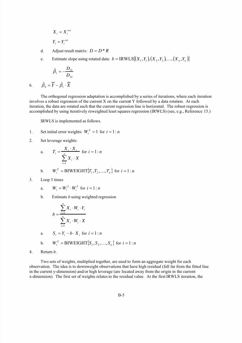
8/11/2019 Battery Life Verification Test Manual
http://slidepdf.com/reader/full/battery-life-verification-test-manual 85/133
B-5
rot
ii X X =
rot
ii Y Y =
d. Adjust result matrix: R D D *=
e. Estimate slope using rotated data: ( ) ( ) ( ) nn Y X Y X Y X b ,,,,,,IRWLS 2211 …
=
22
121
ˆ D
D−= β
6. X Y ⋅−= 10ˆˆ β β
The orthogonal regression adaptation is accomplished by a series of iterations, where each iteration
involves a robust regression of the current X on the current Y followed by a data rotation. At each
iteration, the data are rotated such that the current regression line is horizontal. The robust regression is
accomplished by using iteratively reweighted least squares regression (IRWLS) (see, e.g., Reference 15.)
IRWLS is implemented as follows.
1. Set initial error weights: 1=S
iW for ni :1=
2. Set leverage weights:
a.
∑=
⋅
⋅=
n
i
i
ii
i
X X
X X T
1
for ni :1=
b. n
T
i T T T W ,,,BIWEIGHT 21 …= for ni :1=
3. Loop 3 times
a. T
i
S
ii W W W ⋅= for ni :1=
b. Estimate b using weighted regression
∑
∑
=
=
⋅⋅
⋅⋅=
n
i
ii
n
i
iii
X W X
Y W X
b
1
1
a. iii X bY S ⋅−= for ni :1=
b. n
S
i S S S W ,,,BIWEIGHT 21 …= for ni :1=
4. Return b.
Two sets of weights, multiplied together, are used to form an aggregate weight for each
observation. The idea is to downweight observations that have high residual (fall far from the fitted line
in the current y-dimension) and/or high leverage (are located away from the origin in the current
x-dimension). The first set of weights relates to the residual value. At the first IRWLS iteration, the

8/11/2019 Battery Life Verification Test Manual
http://slidepdf.com/reader/full/battery-life-verification-test-manual 86/133
B-6
residual weights are uniformly set to one. In the two IRWLS iterations that follow, the residual weights
depend on how far off the predicted y-dimension is from the observed y-dimension in the previous fit.
The leverage weights for an observation depend on how far in the current x-dimension the observation is
from zero. The leverage weights remain constant over the three IRWLS iterations.
Both the residual and leverage weights are obtained using Tukey’s biweight function (e.g., see
Reference 16), with c = 6. Let n Z Z Z ,,,BIWEIGHT 21 …
represent the biweight function and its
generic arguments.
1. Compute median absolute value of Zi’s: MAV
2. Compute standardized values of Zi’s: ( ) MAV c Z
U ii ⋅=
3. 1if 0 ≥= ii Z WEIGHT for ni :1=
4. ( ) 1if 122 <−= iii Z U WEIGHT for ni :1=
5. Return WEIGHTs.
The estimation of ASI O is as follows. For each RPT (value of t ), the average ASI value across all
test cells is computed. Denote these average values by ,,, 10 N I S A I S A I S A … . The estimate of ASI O
is given by:
( )
⎟⎟⎟⎟
⎠
⎞
⎜⎜⎜⎜
⎝
⎛
⋅⎪⎭
⎪⎬⎫
⎪⎩
⎪⎨⎧
⎟⎟ ⎠
⎞⎜⎜⎝
⎛
−⋅⎥
⎦
⎤⎢⎣
⎡+−⋅−=
∑∑ ∑
=
= = N
i
k
N
i
N
i
k
i N I S A I S A
0
1
0 10
100
ˆ
1
1ˆ
11ˆˆˆ
β β
β β .
B-1.3 Estimation of Life on Test
The life on test estimate is obtained via the estimated ROR model parameters, ∆t RPT , and PF (which
is the maximum allowable fraction of degradation). The life on test estimate is
( ) ( )
( ) ( )[ ]
⎪⎭
⎪⎬⎫
⎪⎩
⎪⎨⎧
⋅−+−⎥⎥⎦
⎤
⎢⎢⎣
⎡
⎟⎟ ⎠
⎞⎜⎜⎝
⎛
−⋅−+⋅
∆= 010
0
10
1
ˆ1ˆˆlog1
ˆ1ˆˆlog
ˆlog
ˆ I S APF
I S At L RPT
TEST β β β β β
.
B-1.4 Use of the Bootstrap Method for Estimating Uncertainties of
Model Parameters and Life on TestThe uncertainty of the various estimated model parameters and life on test can be assessed by using
the bootstrap, which is a procedure for estimating the uncertainty associated with complex estimation
procedures. The motivation for using the bootstrap here is the complex nature of the estimation
procedure ROR, for which it is difficult to analytically derive a useful estimate of the standard errors for
the model parameters: ASI 0, β ο , and β 1 .

8/11/2019 Battery Life Verification Test Manual
http://slidepdf.com/reader/full/battery-life-verification-test-manual 87/133
B-7
While the bootstrap is applied here for ROR with the given model, it is intended to be a general
methodology for obtaining useful confidence limits for a quantity produced by any model and data
analysis method used by a developer. Thus, it should be useful even in the absence of specific
information on what developers might use in the future.
A simple way to think of the bootstrap is that it is a procedure for creating multiple realizations of
experimental data from the single realization of actual data. In fact, one can view the bootstrap as asimulation using the experimental data. The bootstrap creates the multiple data realizations by sampling
“with replacement.” The data analysis is then performed separately on each data realization resulting in aquantity of interest (e.g., “life on test”) for each realization.
Given the estimates of the three model parameters, we estimate m ASI ASI ASI ASI ,,,, 321 …
recursively using the relationship 110ˆˆˆˆ
−⋅+= k k I S A I S A β β . Next, we compute the differences between
the elements of m I S A I S A I S A I S A ˆ,,ˆ,ˆ,ˆ210 … and imiii ASI ASI ASI ASI ,,,, 210 … for all values of i.
Denote these differences as nmnnmm eeeeeeeee ,,,,,,,,,,,,, 102212011110 ………………=e and the average
error for the ith cell as ie (i.e., imiii eeeavge ,,, 10 …= ). Define measurement error as
nnmnnm eeeeeeee −−−−= ,,,,,, 011110 ……… f .
The ie ’s represent cell-specific effects (cell-specific ohmic and electrode area effects (see
Section 2 of the manual). The values of k I S A ˆ (k=0, 1, 2, ..., m), the ie ’s, and the elements of f are the
essential ingredients of the bootstrap.
The bootstrap procedure suggested here assumes that m I S A I S A I S A I S A ˆ,,ˆ,ˆ,ˆ210 … represents
“truth.” The set of “measurement errors” to draw from is given by e. The bootstrap procedure constructs
a number of artificial data sets (say N ), from which the model parameters and other statistics (e.g., life on
test) are estimated. Each data set is constructed as follows:
1. Draw n samples from , , ,1 2
e e en… with replacement: , , ,1 2
E E E n… . These values become
simulated cell-specific effects.
2. Draw n samples of size m+1 from f with replacement: 0 1, , , 1:i i imF F F F for i n= =…
i. This is
the simulated measurement error.
3. Form a simulated ASI data set. Simulate the observed ASI measurements of the ith cell by adding
E i and F i to ˆ ˆ ˆ ˆ, , , ,0 1 2
ASI ASI ASI ASI m… .
4. Using ROR on simulated data set, get estimates of the parameters:
( ) ( )boot boot I S A 10ˆ and bootˆ),(ˆ β β
.
5. Estimate the life on test (LOT(boot)) given: ( )0ˆ ASI boot , ( ) ( )0 1
ˆ ˆ boot , and boot β β .
This 5-step process is repeated N boot times to give N boot values for ( )boot I S A 0ˆ ,
( ) ( )0 1ˆ ˆ boot , and boot β β as well as ( )boot LTEST
ˆ . A suggested value for N boot is 100.

8/11/2019 Battery Life Verification Test Manual
http://slidepdf.com/reader/full/battery-life-verification-test-manual 88/133
B-8
The bootstrap standard error for any of these quantities is simply the standard deviation of the
quantities taken over the N boot bootstrap simulations (e.g.,)(ˆ boot T O L
S ). Confidence intervals for any of
these quantities can be derived directly from percentiles of the empirical distributions of the bootstrapestimates.
B-2. Example Use of the Data Analysis Methods Applied to Advanced Technology Development L ife Test Data
Testing of the second generation of ATD cells (i.e., Gen 2 cells) is nearing completion. These
18650-size cells, consisting of both a baseline and variant chemistry, have been distributed over a matrix
consisting of several SOCs, temperatures, and life tests (Reference 2). Life testing is performed inaccordance with the PNGV Battery Test Manual (Reference 19), with interruptions every 4 weeks for
reference performance tests (RPTs). The L-HPPC test is regularly included as part of the Gen 2 RPT, and
is used to calculate changes in ASI as a function of test time (the Gen 2 discharge ASI data are based on
the 18-s pulse at a 5C rate, as defined in Reference 19).
B-2.1 Background
The data analysis methods for modeling battery life test data presented above are the results of
intensive efforts to analyze such data from the Advanced Technology Development program. The data
set first used was from cycle-life testing of Gen 2 Baseline cells at 45ºC. One approach involved a formof auto-correlation to quantify the sources of variation in the measured ASI for this group of cells
(Reference 12). The values of pulse power measured at four weeks (Y-coordinate) were plotted against
the corresponding values measured in the initial cell characterization (X-coordinate). This form of scatter
plot revealed a linear relationship between the two variables, with a high positive correlation coefficient
(+0.96). Extension of the method to Variant C cells in cycle-life testing at 45ºC, and to cells in calendar-
life testing at 45ºC, gave similar results.
The implications of this linear relationship were not immediately clear. Analysis of the linear
regression using an iterated solution from a Taylor-series expansion led finally to the general solution presented previously:
ASIt+∆t RPT = β O + β 1 ASIt
ASIt = [ β O + ( β 1 – 1) ASIt=0] exp[ln( β 1) t/ ∆t RPT ] – β O / ( β 1 – 1) .
This basic approach to the modeling of ASI test data was subsequently refined into its present state
of development, as illustrated in the following.
B-2.2 Appl ication to the Gen 2 Cycle-Life Data
Figure B-1 shows the ASI as a function of test time for all of the Baseline cells cycle-life tested at
25°C, and the observed linear relationship for these cells between the values at time t+∆t and t weeks is
shown in Figure B-2. Figure B-3 shows the ASI as a function of test time for the 45°C cycle-life Baseline
cells. Both the 25 and 45°C cells were cycled using the 25-Wh power assist profile with RPTs every
33,600 cycles. Each temperature group began with 14 cells, but pairs of cells were removed at regular
power fade increments for diagnostic analysis (Reference 2). Consequently, only four 25°C Baseline
cells have been testing beyond 72 weeks. These cells have completed 112 weeks of cycling, and will
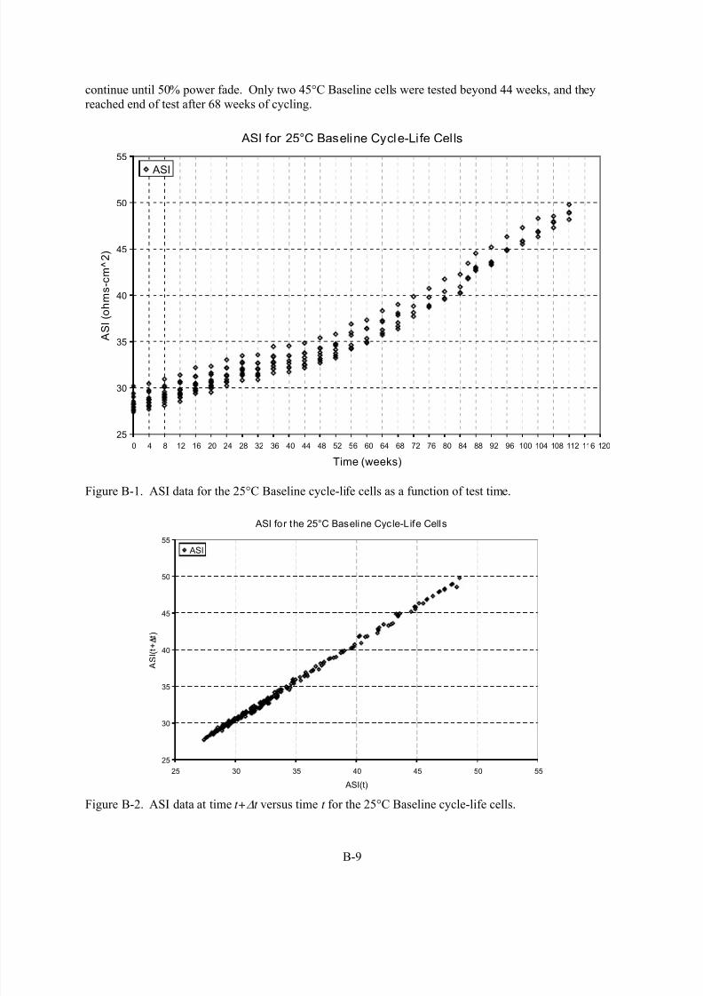
8/11/2019 Battery Life Verification Test Manual
http://slidepdf.com/reader/full/battery-life-verification-test-manual 89/133
B-9
continue until 50% power fade. Only two 45°C Baseline cells were tested beyond 44 weeks, and they
reached end of test after 68 weeks of cycling.
ASI for 25°C Baseline Cycle-Li fe Cells
25
30
35
40
45
50
55
0 4 8 12 16 20 24 28 32 36 40 44 48 52 56 60 64 68 72 76 80 84 88 92 96 100 104 108 112 116 120
Time (weeks)
A S I ( o h m s - c m ^ 2 )
ASI
Figure B-1. ASI data for the 25°C Baseline cycle-life cells as a function of test time.
ASI for the 25°C Baseline Cyc le-Life Cells
25
30
35
40
45
50
55
25 30 35 40 45 50 55
ASI(t)
A S I ( t + t )
ASI
Figure B-2. ASI data at time t+∆t versus time t for the 25°C Baseline cycle-life cells.

8/11/2019 Battery Life Verification Test Manual
http://slidepdf.com/reader/full/battery-life-verification-test-manual 90/133
B-10
ASI for 45°C Baseline Cycle-Life Cells
25
30
35
40
45
50
55
0 4 8 12 16 20 24 28 32 36 40 44 48 52 56 60 64 68 72
Time (weeks)
A S I ( o h m s - c m ^ 2 )
ASI
Figure B-3. ASI data for the 45°C Baseline cycle-life cells as a function of test time.
Figure B-4 shows the 25°C Baseline cell ASI at time t+∆t as a function of the ASI at time t . As
mentioned above, the data are very linear, and, consequently, the ROR fit to the data is in excellent
agreement. Also shown are the aggregate weights (the product of the residual and leveraging weights) for
each observation. As discussed above, the early and late data are high leverage points, and so are down-
weighted to avoid possible detrimental influences to the slope ( β 1).
Figure B-5 shows the ROR fit for the 45°C Baseline cycle-life cells. Unlike the 25°C cells, these
data do not show a simple linear relationship. The initial characterization data [with an ASI(t) less then
30 ohm-cm2] are offset compared to the remaining ASIs. This may be primarily due to improper
formation cycling, as discussed in Reference 1 and Appendix C. Therefore, these data need to be ignored
in the ROR analysis for more accurate life on test projections. The 45°C data also showed a mechanistic
change, with a higher rate of degradation, after 32 weeks of aging (Reference 2). Consequently, the ROR
analysis also had to be split into two components at 32 weeks. As shown in Figure B-5, the two ROR fits
match their respective data sets more accurately than a single ROR fit would be able to accomplish.
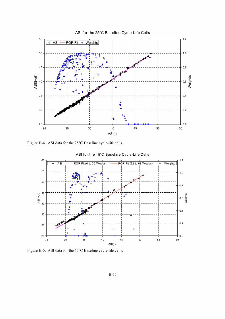
8/11/2019 Battery Life Verification Test Manual
http://slidepdf.com/reader/full/battery-life-verification-test-manual 91/133
B-11
ASI for the 25°C Baseline Cyc le-Life Cells
25
30
35
40
45
50
55
25 30 35 40 45 50 55
ASI(t)
A S I ( t +
t )
0.0
0.2
0.4
0.6
0.8
1.0
1.2
W e i g h t s
ASI ROR Fit Weights
Figure B-4. ASI data for the 25°C Baseline cycle-life cells.
ASI for the 45°C Bas el in e Cyc le-L ife Cel ls
25
30
35
40
45
50
55
60
25 30 35 40 45 50 55 60
ASI(t )
A S I ( t + d t )
0.0
0.2
0.4
0.6
0.8
1.0
1.2
W e i g h t s
ASI ROR Fit (0 to 32 W eeks) ROR Fit (32 to 68 W eek s) Weights
Figure B-5. ASI data for the 45°C Baseline cycle-life cells.
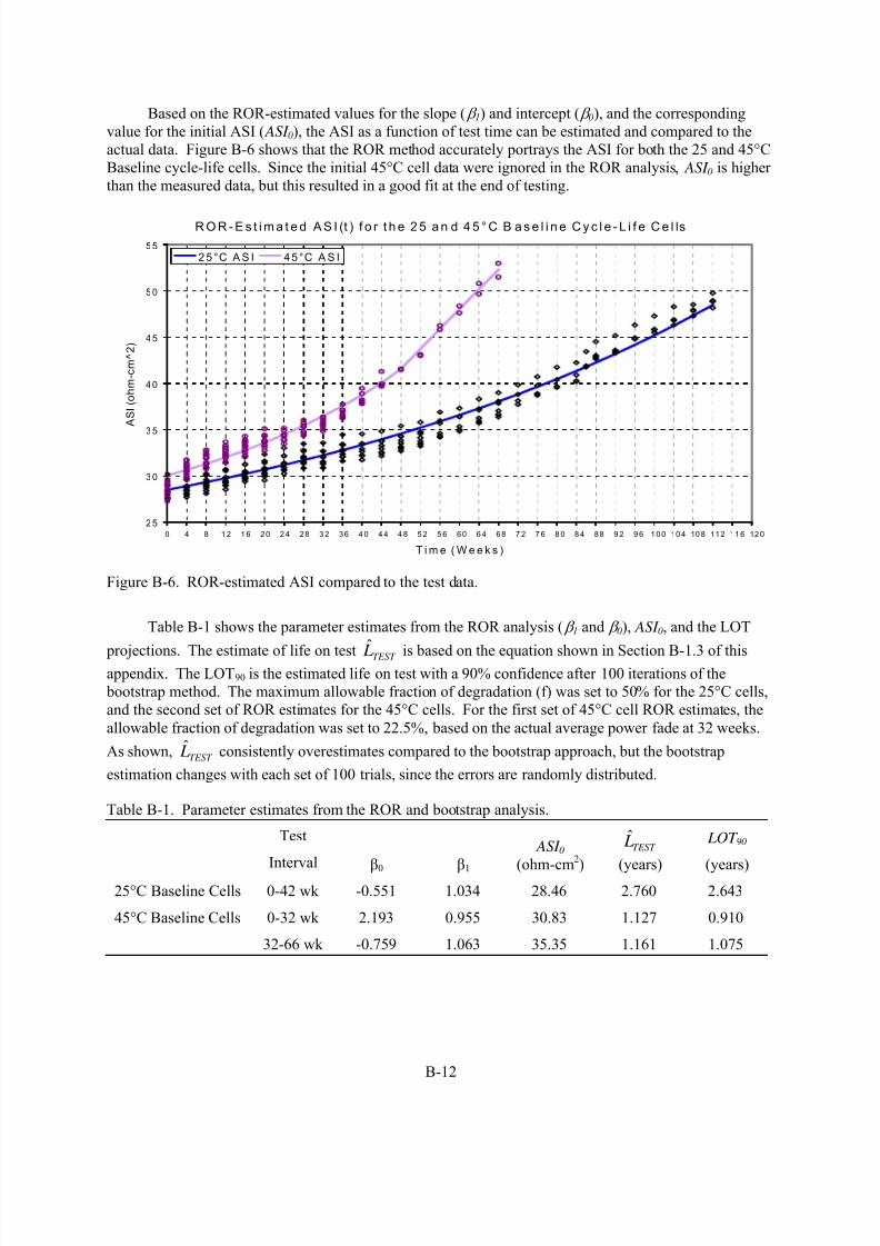
8/11/2019 Battery Life Verification Test Manual
http://slidepdf.com/reader/full/battery-life-verification-test-manual 92/133
B-12
Based on the ROR-estimated values for the slope ( β 1) and intercept ( β 0), and the corresponding
value for the initial ASI ( ASI 0), the ASI as a function of test time can be estimated and compared to the
actual data. Figure B-6 shows that the ROR method accurately portrays the ASI for both the 25 and 45°C
Baseline cycle-life cells. Since the initial 45°C cell data were ignored in the ROR analysis, ASI 0 is higher
than the measured data, but this resulted in a good fit at the end of testing.
R O R - E s t i m a t e d A S I (t ) f o r t h e 2 5 a n d 4 5 ° C B a s e l i n e C y c l e - L i f e C e l ls
25
30
35
40
45
50
55
0 4 8 12 16 20 24 28 32 36 40 44 48 52 56 60 64 68 72 76 80 84 88 92 96 100 104 108 112 116 120
T i m e ( W e e k s )
A S I ( o h m - c m ^ 2 )
2 5°C A S I 45°C A S I
Figure B-6. ROR-estimated ASI compared to the test data.
Table B-1 shows the parameter estimates from the ROR analysis ( β 1 and β 0), ASI 0, and the LOT
projections. The estimate of life on test TEST Lˆ
is based on the equation shown in Section B-1.3 of thisappendix. The LOT90 is the estimated life on test with a 90% confidence after 100 iterations of the
bootstrap method. The maximum allowable fraction of degradation (f) was set to 50% for the 25°C cells,
and the second set of ROR estimates for the 45°C cells. For the first set of 45°C cell ROR estimates, the
allowable fraction of degradation was set to 22.5%, based on the actual average power fade at 32 weeks.
As shown, TEST L consistently overestimates compared to the bootstrap approach, but the bootstrap
estimation changes with each set of 100 trials, since the errors are randomly distributed.
Table B-1. Parameter estimates from the ROR and bootstrap analysis.
Test
Interval β0
β1
ASI 0(ohm-cm2)
TEST L
(years)
LOT 90
(years)
25°C Baseline Cells 0-42 wk -0.551 1.034 28.46 2.760 2.643
0-32 wk 2.193 0.955 30.83 1.127 0.91045°C Baseline Cells
32-66 wk -0.759 1.063 35.35 1.161 1.075

8/11/2019 Battery Life Verification Test Manual
http://slidepdf.com/reader/full/battery-life-verification-test-manual 93/133
B-13
B-2.3 Effects of Temperature Sensit ivity
Temperature sensitivity is an important issue in estimating life on test, and the MPPC has been
designed to allow for temperature compensations at each RPT interval (Section 3.1.2.2). Although the
Gen 2 RPT was not designed for continuous temperature adjustments, a methodology has been developed
to compensate for temperature fluctuations on the cycle-life Baseline cell data to determine the effects of
temperature on life on test estimations. The Gen 2 data were adjusted using the equations defined in
Section 4.1.3, with a linearly increasing T ASI . The T ASI coefficient was determined from the Arrhenius
slope of the cycle-life pulse resistances based on similar average ASIs, but at different RPT intervals.
Figure B-7 shows the ROR-estimated ASI as a function of test time for the temperature
compensated data compared to the original estimations (also shown in Figure B-6). Table B-2 shows the
parameter estimates and bootstrap analysis from the adjusted data. For the first set of the 45°C cells, the
allowable fraction of degradation was set to 21.0%, based on the average adjusted power fade at 32
weeks. As shown, the impact of temperature results in small changes to the life on test estimations.
ROR-Estimated ASI for the 25 and 45°C Baseline Cycle-Life Cells
25
30
35
40
45
50
55
0 4 8 12 16 20 24 28 32 36 40 44 48 52 56 60 64 68 72 76 80 84 88 92 96 100 104 108 112 116 120
Time (weeks)
A S I ( o h m - c m ^ 2 )
25°C ASI (Original)
25°C ASI (Adjusted)
45°C ASI (Original)
45°C ASI (Adjusted)
45°C Cells
25°C Cells
Figure B-7. ROR-estimated ASI for the measured and adjusted ASI data.
Table B-2. Parameter estimates from the ROR and bootstrap analysis of the adjusted data.
Test
Interval β0 β1
ASI0
(ohm-cm2)
TEST L
(years)
LOT90
(years)
25°C Baseline Cells 0-42 wk -0.717 1.039 28.49 2.642 2.500
0-32 wk 2.464 0.946 30.57 1.089 0.81845°C Baseline Cells
32-66 wk 1.320 1.012 34.27 1.359 1.201

8/11/2019 Battery Life Verification Test Manual
http://slidepdf.com/reader/full/battery-life-verification-test-manual 94/133
B-14
B-2.4 Noise Levels
Figure B-8 shows the cell-to-cell residual ASI error for the four longest lasting 25°C Baseline
cycle-life cells. The residual error was determined based on the difference between the actual cell ASI
and the estimated ASI from the ROR analysis for each individual cell. The noise is somewhat correlated,which reduces the effectiveness of adding cells to reduce the noise. (Noise would be reduced by a factor
of 1 N for uncorrelated noise using N cells.)
ATD Gen 2 BL Cells in Cycle Life at 25oC
Correlations of Residual ASI Errors for the 4 Oldest Cells
R2 = 0.7934
R2 = 0.7627
R2 = 0.9325
R2 = 0.5638
R2 = 0.7656
R2 = 0.9022
-1.2
-1.0
-0.8
-0.6
-0.4
-0.2
0.0
0.2
0.4
0.6
0.8
1.0
1.2
-1.2 -1.0 -0.8 -0.6 -0.4 -0.2 0.0 0.2 0.4 0.6 0.8 1.0 1.2
Residual ASI Error for Cell #1
R e s i d u a l A S I E r r o r f o r C e l l # 2
Cell 111 vs. 109
Cell 114 vs. 109
Cell 115 vs. 109
Cell 114 vs. 111
Cell 115 vs. 111
Cell 115 vs. 114
Figure B-8. Correlations of residual errors.

8/11/2019 Battery Life Verification Test Manual
http://slidepdf.com/reader/full/battery-life-verification-test-manual 95/133
C-1
Appendix C
Study of Li fe-Limiting Mechanisms in High-Power Lithium-Ion Cells

8/11/2019 Battery Life Verification Test Manual
http://slidepdf.com/reader/full/battery-life-verification-test-manual 96/133

8/11/2019 Battery Life Verification Test Manual
http://slidepdf.com/reader/full/battery-life-verification-test-manual 97/133
C-3
Appendix C
Study of Life-Limiting Mechanismsin High-Power Li-Ion Cells
C-1. INTRODUCTION
DOE’s Advanced Technology Development (ATD) program has studied the aging mechanisms
of high-power lithium-ion cell chemistries since it was initiated in 1999. Several cell chemistries
were developed on the ATD program and then studied in high-power 18650 spiral-wound cells.
They were subjected to accelerated aging tests and then extensively investigated using a wide
range of diagnostic tools. All groups of cells studied to date reach end-of-life due to increasing
impedance and corresponding power loss. For the latest high-power cell chemistry (denoted the
Gen 2 cell chemistry), a phenomenological cell model was developed and used to study and
identify possible phenomena that could be limiting specie transport within the cell chemistry and
causing the observed impedance rise during cell aging. The model was used to link the
diagnostic findings to the aging characteristics of the cells. This appendix provides a brief summary of the latest cell chemistry and the studies performed on these cells in an attempt to
identify the main factors responsible for impedance rise and power fade in these cells. Since this
is a cell chemistry that was studied extensively, it is being used as an example of a technology-
specific approach for developing life prediction methodologies, as recommended in this manual.
C-2. GEN 2 CELL DESCRIPTION
The Gen 2 cells are of the standard 18650 size, however they were custom designed for high
power and for better hermeticity. They employ 10 tabs along the length of both the positive and
negative electrodes. This significantly reduces the resistance associated with the current
collection system during high-current charge and discharge pulses. Also, the cells employ an
aluminum case, which is connected to the positive electrode, and the cells are sealed via a laser weld. All cells were leak checked to ensure a high degree of hermeticity, prior to being shipped.
Table C-1 lists the cell chemistry that was employed in the ATD Gen 2 baseline cells. The
electrode materials were selected on the basis of material screening tests of advanced low-cost
materials available from international suppliers in 2000. The electrolyte formulation was
developed jointly by Argonne National Laboratory (ANL) and the U.S. Army Research
Laboratory (ARL) and made for the ATD program by Quallion, LLC, the same company that
designed and built the Gen 2 high-power 18650 cells (to ANL specifications).
Table C-1. Gen 2 Baseline Cell Chemistry
Positive Electrode:
84 wt% LiNi0.8Co0.15Al0.05O2 (Fuji CA1505)8 wt% PVdF binder (Kureha KF-1100)
4 wt% SFG-6 graphite (Timical)
4 wt% carbon black (Chevron)
8 mg/cm2 loading density
35 µm thick coating /side
30 µm thick Al current collector
Negative Electrode:
92 wt% MAG-10 graphite (Hitachi)8 wt% PVdF binder (Kureha #C)
4.9 mg/cm2 loading density
35 µm thick coating/side
18 µm thick Cu current collector
Electrolyte:
1.2M LiPF6 in EC:EMC (3:7)
Separator:
25 µm thick polyethylene (Celgard)

8/11/2019 Battery Life Verification Test Manual
http://slidepdf.com/reader/full/battery-life-verification-test-manual 98/133
C-4
A second group of cells were built using a very similar cell chemistry. The only difference in the
chemistry was the level of aluminum dopant in the positive electrode active material—the level of
aluminum was increased from 5% to 10%. This material was also produced by Fuji Chemical,
using the same spray drying process that was used for making the positive electrode material for
the Gen 2 baseline cells and both materials were subjected to the same calcination process. This
second group of cells is denoted the Gen 2 Variant C cells.
C-3. ACCELERATED AGING TESTS
A total of 165 cells were built using the Gen 2 baseline cell chemistry described above. Most of
the cells were used in accelerated tests and in studying acceleration parameters, while others were
used in abuse tolerance testing. Forty-seven cells went to cycle and calendar life testing at the
Idaho National Engineering and Environmental Laboratory (INEEL) and ANL, respectively.
Fourteen cells were cycle life tested at 25oC, fourteen cells were cycle life tested at 45oC, and 14
cells were calendar life tested at 55oC. Two additional cells were put on calendar life test at 45oC.
Three cells were simply characterized before being sent to the diagnostics labs (ANL,
Brookhaven National Laboratory, and Lawrence Berkeley National Laboratory) for benchmark
evaluation. Another 30 cells were made with Variant C chemistry. Several of these cells arrived
at ANL with soft shorts and were set aside. Of those that passed the initial characterization tests,
14 were put on cycle life test at 45oC and 10 were put on calendar life test at 45oC. The test
regime and the laboratory responsible for the testing are given in Table C-2.
Table C-2. Gen 2 Cell Test Conditions
Testing Laboratory Baseline Cells Variant C Cells
Calendar Cycle Calendar Cycle
ANL 14 cells - 55oC
2 cells - 45oC
10 cells - 45oC
INEEL 14 cells - 25oC
14 cells - 45oC
14 cells - 45oC
(Calendar- and cycle-life testing were performed at 60% SOC, which, based on the initial C1/25
tests, corresponded to 3.723 and 3.741 V for baseline and Variant C cells, respectively.)
The calendar-life cells were subjected to a daily 3C current pulse at temperature for 28
consecutive days to monitor cell impedance changes, as defined in the test manual.16 The cycle-
life cells were aged using the BSF-scaled, 25-Wh profile of Reference 19. Before cycle-life
testing, the operating set point stability (OSPS) test was performed to verify cycling stability.
The OSPS test consists of 100 consecutive cycle-life profiles. The requirement is that at its
completion, the actual SOC should be within ±2% of 60% SOC, based on the OCV following a 1-
h rest at the beginning and end of the 100 pulses. If the SOC is charge positive or charge
negative (i.e., unstable), then the control voltage at the end of the discharge pulse is changed and
the OSPS test is repeated until stable cycling occurs.
As shown in Table C-2, the cycle-life cells were tested at 25 and 45oC. After four weeks at
temperature (33,600 profiles), RPTs were performed, as described below. End-of-life for these
cells was defined as 30% power fade. Throughout the testing, selected cells were removed at
predetermined intervals and forwarded to the diagnostic team for tear down and evaluation. At
first, two cells were removed after 4 weeks of testing. The removal scheme was then changed to
depend on power fade increments. For the baseline cells, the increments were approximately
5.2% and 3.6% for the cycle life cells at 25 and 45oC, respectively. For the baseline calendar life

8/11/2019 Battery Life Verification Test Manual
http://slidepdf.com/reader/full/battery-life-verification-test-manual 99/133
C-5
cells at 55oC, the increment was approximately 3.6%. For the Variant C cycle life cells, the
power fade increment was approximately 3%; and for the calendar life cells, it was approximately
3.6%. Thus, by 30% power fade, 12 cells were removed from test. The final two cells were left
on test until 50% power fade. The two calendar life tested cells at 45oC were left on test for the
full 50% power fade. The power values used in these removal schemes were defined by the
intersection of the curve for a given cell and the 300-Wh line on the Available Energy vs. Power
graph, as defined in the test manual.16
For all cells, RPTs were performed at 4-week intervals, but, at first, not all cells received the full
RPT given in Table C-3. In the time interval of 4 to 12 weeks, only two selected cells, plus any
that were scheduled for removal, received the full RPT. The more-limited RPT omitted the EIS
and C/25 experiments. At 16 weeks and thereafter, all cells received the full RPT. The RPT for
these test cells was more extensive than the RPTs found in the FreedomCAR test manuals. The
reason for this was to extract as much electrochemical information as reasonably possible during
aging. A description of the low-current hybrid pulse power characterization (L-HPPC) test is
provided in Reference 19.
Table C-3. ATD Reference Performance Test Sequence
Temperature (oC) ANL (Calendar Life) INEEL (Cycle Life)25 C1/1 discharge C1/1 discharge
25 C1/25 discharge L-HPPC
25 C1/25 charge C1/25 discharge
25 EIS at 60% SOC C1/25 charge
25 L-HPPC EIS at 60% SOC
As the cells age, the C/25 capacity fades. A plot of the average C/25 capacity versus time for the
cells along with the least squares fit to at 1/2
+ d is given in Figure C-1. From the values of r 2, 0.96
to 1.00, the fits are excellent. The order of C/25 capacity fade is 55oC calendar life > baseline
cycle life at 45oC ≈ baseline calendar life at 45oC > Variant C calendar life at 45oC ≥ Variant C
cycle life at 45oC ≈ 25oC cycle life. The fact that all the curves can be fit to a t 1/2-dependent
equation (parabolic kinetics) indicates that there is a common, diffusion-controlled, lithium-
consuming reaction occurring in both chemistries, such as a lithium corrosion reaction at the
anode.
The time-dependent behavior of the C/1 capacity is more complex (see Figure C-2). Instead of a
smooth curve, the curves have breaks in them which change, primarily, with temperature. As will
be shown below, the breaks in the curves from the baseline cells can be attributed to the changes
in the ASI.
As the cells age, the area-specific impedance (ASI) increases. Plotting the ASI values at 60%
SOC vs. time shows that there are cathode-dependent (i.e., Al content) differences in the way ASI
increases. This is shown in Figure C-3. The baseline chemistry follows a two-step mechanism
that depends on t 1/2 at first then on t at later times. In this experiment, temperature controls only
where the change from t 1/2 to t occurs. The data from the Variant C cells shows that ASI also
depends on t 1/2 and on t . The change in time dependency appears in the long-term aging data; it
occurs later in cell life (35 vs. 55 weeks, respectively, for baseline and Variant C chemistries).
Since the only known difference between the two cell chemistries is the composition of the
cathode, the cathode could play a significant role in the cell impedance rise. The fact that the
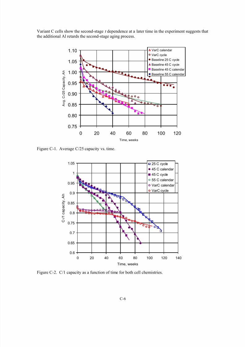
8/11/2019 Battery Life Verification Test Manual
http://slidepdf.com/reader/full/battery-life-verification-test-manual 100/133
C-6
Variant C cells show the second-stage t dependence at a later time in the experiment suggests that
the additional Al retards the second-stage aging process.
0.75
0.80
0.85
0.90
0.95
1.00
1.05
1.10
0 20 40 60 80 100 120
Time, weeks
A v g .
C 1 / 2 5 C a p a c i t y ,
A h
VarC calendar
VarC cycle
Baseline 25 C cycleBaseline 45 C cycle
Baseline 45 C calendar
Baseline 55 C calendar
Figure C-1. Average C/25 capacity vs. time.
0.6
0.65
0.7
0.75
0.8
0.85
0.9
0.95
1
1.05
0 20 40 60 80 100 120 140
Time, weeks
C 1 / 1 c a p a c i t y ,
A h
25 C cycle
45 C calendar
45 C cycle
55 C calendar
VarC calendar
VarC cycle
Figure C-2. C/1 capacity as a function of time for both cell chemistries.

8/11/2019 Battery Life Verification Test Manual
http://slidepdf.com/reader/full/battery-life-verification-test-manual 101/133

8/11/2019 Battery Life Verification Test Manual
http://slidepdf.com/reader/full/battery-life-verification-test-manual 102/133
C-8
The data in Figure C-3 shows that, sometimes, the transition from one mechanism to another is
obvious and, at other times, it is subtle. Good examples of obvious transitions are the ASI data
from the baseline cells. An example of a subtle change is illustrated by the ASI data from the
Variant C cycle life cells. Replotting the data on log-log axes helps elucidate the change in
mechanism. Examples are shown in Figure C-4, using the data mentioned. If the data had
followed one mechanism, the plot on the log-log axes will be a straight line, with the slopedependent on the exponent of time. From Figure C-4, the curves are not linear, indicating that the
exponent of time has changed. Hence, there is a change in mechanism.
Additional information was obtained from EIS experiments. A typical EIS spectrum is given in
Figure C-5. From this figure, the high-frequency minimum does not change appreciably with
time. Proceeding to lower frequencies, the real part of the impedance of the next local minimum
increases with time. Finally, the length of the low-frequency tail seems to be increasing with
time. The mid-frequency arc is typically associated with interfacial impedance, while the low-
frequency tail is typically associated with diffusional impedance.
The mid-frequency-range data in Figure C-5 (through interfacial arc) were modeled using the
equivalent circuit shown in Figure C-6. The results show that R1 (materials resistance) does notincrease significantly. This is also apparent in Figure C-5. The other two resistances, R2 and R3,
representing interface impedance, change with time. A plot of these values is shown in Figure
C-7. From the plot, R2 increases linearly with time while R3 increases non-linearly, similar to
that seen in Figure C-3. The shape of the ASI data is, in part, due to the behavior of R2+R3.
A separate study was conducted to examine the importance of various acceleration factors on the
aging characteristics of the Gen 2 baseline cells. Since, these tests were conducted using different
protocols and different RPTs, data from those tests are not directly comparable and are not
included here to avoid confusion. However, these tests clearly showed that cell state-of-charge
(SOC) was another parameter that had a significant impact on the rate of impedance rise andcapacity fade in the Gen 2 cells (Reference 21).
25
27
29
31
33
35
37
39
41
43
45
25 27 29 31 33 35 37 39 41 43
ASI t, ohm-cm2
A S I t + 4 , o h m - c m
2
Figure C-3a. Plot of the initial ROR analysis results using the baseline calendar at 55oC data.
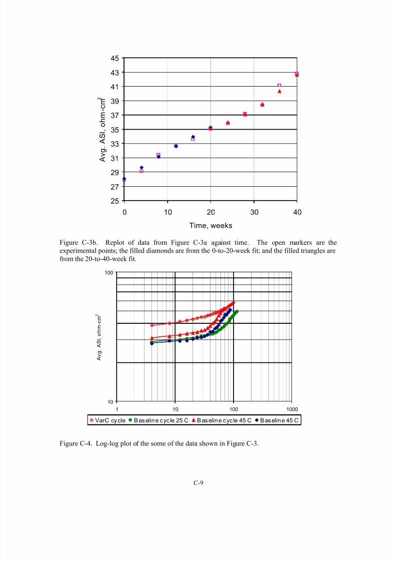
8/11/2019 Battery Life Verification Test Manual
http://slidepdf.com/reader/full/battery-life-verification-test-manual 103/133
C-9
25
27
29
31
33
35
37
39
41
43
45
0 10 20 30 40
Time, weeks
A v g .
A S I , o h m - c m
2
Figure C-3b. Replot of data from Figure C-3a against time. The open markers are the
experimental points; the filled diamonds are from the 0-to-20-week fit; and the filled triangles are
from the 20-to-40-week fit.
10
100
1 10 100 1000
Time, week s
A v g .
A S I , o h m - c m
2
VarC cycle Baseline cyc le 25 C Baseline cyc le 45 C Baseline 45 C
Figure C-4. Log-log plot of the some of the data shown in Figure C-3.

8/11/2019 Battery Life Verification Test Manual
http://slidepdf.com/reader/full/battery-life-verification-test-manual 104/133
C-10
0
0.005
0.01
0.015
0.02
0.025
0.03
0 0.01 0.02 0.03 0.04 0.05 0.06
Zreal, ohms
- Z i m a g , o h m s
Characterization t = 0RPT #1 t = 4 weeksRPT #2 t = 8 weeksRPT #3 t = 12 weeksRPT #4 t = 16 weeksRPT #5 t = 20 weeksRPT #6 t = 24 weeksRPT #7 t = 28 weeksRPT #8 t = 32 weeksRPT #9 t = 36 weeks
RPT #10 t = 40 weeksRPT #11 t = 44 weeksRPT #12 t = 48 weeksRPT #13 t = 52 weeksRPT #14 t = 56 weeksRPT #15 t = 60 weeksRPT #16 t = 64 weeksRPT #17 t = 68 weeksRPT #18 t = 72 weeksRPT #19 t = 76 weeksRPT #20 t = 80 weeksRPT #21 t = 84 weeksRPT #22 t = 88 weeks
45oC
Figure C-5. Typical Nyquist plot from a baseline calendar life cell tested at 45oC. The plots from
the cycle life and Variant C cells are similar in appearance.
R1C1
R3
CPE1
R2
Figure C-6. Equivalent circuit used for modeling the data in Figure C-4.
R2 = 0.98
0
0.003
0.006
0.009
0.012
0.015
0.018
0.021
0.024
0.027
0.03
0 10 20 30 40 50 60 70 80
Time, weeks
R e s i s t a n c e , o h m s
0
0.003
0.006
0.009
0.012
0.015
R e s i s t a n c e , o h m s
R2
R3
Figure C-7. Values of two of the equivalent circuit model parameters, R2 and R3, vs. time.

8/11/2019 Battery Life Verification Test Manual
http://slidepdf.com/reader/full/battery-life-verification-test-manual 105/133
C-11
C-4. ELECTROCHEMICAL DIAGNOSTICS
In an effort to identify the sources of capacity fade and impedance rise, electrochemical tests were
conducted on electrodes harvested from 18650-cells that showed varying levels of performance
degradation. Coin cells (2032-type) were assembled with 1.6-cm2 area samples punched from the
harvested electrodes, lithium-metal counter electrode, fresh Celgard 2325 separator, and fresh
1.2M LiPF6 + EC:EMC (3:7) electrolyte to determine the effect of aging on electrode capacity.
The cells containing the positive electrode (cathode) were cycled thrice from 3 to 4.3 V, and the
cells containing the negative electrode (anode) were cycled thrice from 0 to 1.5 V. The cycling
was conducted at various current densities (~C/5 to C/200) to determine the effect of cycling rate
on cell capacity.
Figure C-8 shows representative discharge data measured with a 0.064 mA current (<C/25 rate)
obtained from cells prepared with cathodes harvested from the 18650-cells. It is evident that the
cell capacity is a function of electrode age. For example, the cells prepared with cathodes from
18650-cells that showed 0%, 18% and 30% capacity fade (CF) had capacities of 2.5, 2.0, and
1.8 mAh, respectively. Cycling at slower rates increased capacity, especially for cells containing
highly aged electrodes. However, the capacities were always smaller than those observed for the
control cells (0% capacity and power fade). Because these cells contain a lithium-metal counter
electrode, the capacity decline suggests the following scenarios:
• Oxide particle isolation, which may result from (a) partially insulating films on the oxide
surface that impede lithium motion into the particles, (b) breakup of secondary particles
into fragments that are not in contact with the carbon (electronic conduction) media, and
(c) retreat of carbon away from the particles.
• Oxide particle damage, which may include (a) changes in the layering structure of the
particle bulk, and (b) changes in the ionic conductivity of the Lix Ni1-xO-type layer that
has been observed on the oxide surface.
Figure C-8. Capacity data from cathodes (vs. Li) harvested from 18650-cells; the numbers
indicate capacity fade of the18650-cells.
3
3.2
3.4
3.6
3.8
4
4.2
4.4
0 0.2 0.4 0.6 0.8 1 1.2 1.4 1.6 1.8 2 2.2 2.4 2.6
Capacity, mAh
V o l t a g e ,
V
0%
10%18%
30%
3
3.2
3.4
3.6
3.8
4
4.2
4.4
0 0.2 0.4 0.6 0.8 1 1.2 1.4 1.6 1.8 2 2.2 2.4 2.6
Capacity, mAh
V o l t a g e ,
V
0%
10%18%
30%

8/11/2019 Battery Life Verification Test Manual
http://slidepdf.com/reader/full/battery-life-verification-test-manual 106/133
C-12
Figure C-9 shows representative discharge data measured with a 0.064 mA current (<C/25 rate)
obtained from cells prepared with the graphite anodes harvested from the 18650-cells. In general,
the cells containing anodes from the higher CF cells showed lower capacities. For example, the
capacity of the 0% CF anode cell was ~3.0 mAh, whereas the cell containing the 30% CF showed
a capacity of only 2.4 mAh. The insert in Figure C-9 shows the discharge data after normalizing
for the capacity variations of the different cells. The curves from the various cells lie atop each
other, which suggests that the bulk of the graphite anode is unaffected by cell aging.
Figure C-9. Capacity data from anodes (vs. Li) harvested from 18650-cells; the numbers indicatecapacity fade of the18650-cells. Inset shows same data after normalizing for cell capacity
variations.
Planar type cells, incorporating micro-reference electrodes, were used to isolate the individual
positive and negative electrode contributions to cell impedance. These reference electrode cells
were assembled with 15.5-cm2 electrodes, two Celgard 2325 separators enveloping a Li-Sn
micro-reference electrode, and fresh electrolyte. The individual electrode contributions to the
fairly rapid early-life impedance rise were studied in cells employing fresh one-side coated Gen 2
electrodes. HPPC and AC impedance studies on these cells showed that the early-life impedance
rise is primarily associated with interfacial phenomena that occur at the positive electrode. Mid-
life studies were conducted in reference electrode cells using positive and negative electrode
laminates that were harvested from the 18650-cells. Figure C-10 shows representative AC-impedance and 18-s pulse discharge HPPC data from these reference electrode cells. The HPPC
data clearly indicate that a significant portion of the cell impedance rise occurs at the positiveelectrode. The AC impedance data also indicate that the positive electrode is the main contributor
to cell impedance rise. Furthermore, the main increase of the positive electrode impedance is
observed at the mid-frequency semicircular arc, which is usually associated with charge-transfer
and mass-transfer processes at the electrode-electrolyte interface. These early- and mid-life
reference-electrode data provide fairly strong evidence that the same phenomena are controlling
the cell impedance rise throughout much of the useful life of these cells. In addition, reference
0
0.5
1
1.5
0 0.5 1 1.5 2 2.5 3
Capacity, mAh
V o l
t a g e ,
V
0%18%30%
0
0.5
1
1.5
0 10 20 30 40 50 60 70 80 90 100
Capacity, %
V o l t a g e ,
V
0
0.5
1
1.5
0 0.5 1 1.5 2 2.5 3
Capacity, mAh
V o l
t a g e ,
V
0%18%30%
0
0.5
1
1.5
0 0.5 1 1.5 2 2.5 3
Capacity, mAh
V o l
t a g e ,
V
0%18%30%
0
0.5
1
1.5
0 10 20 30 40 50 60 70 80 90 100
Capacity, %
V o l t a g e ,
V

8/11/2019 Battery Life Verification Test Manual
http://slidepdf.com/reader/full/battery-life-verification-test-manual 107/133
C-13
electrode cells, prepared with electrodes from highly-aged (late-life) 18650 cells, showed
significant Warburg impedances in the AC impedance spectra, which were again primarily
attributable to the positive electrode. These data indicate that late in the life of these 18650-cells
it becomes increasingly difficult to transport lithium into and/or through the oxide particles.
The electrochemical diagnostic studies show fairly conclusively that phenomena occurring at the
positive electrode are controlling the impedance rise and limiting the life of the Gen 2 cells.Therefore, most of the physicochemical diagnostic studies were focused on the positive electrode,
in an effort to identify phenomena than can cause the observed impedance rise. Similarly, early
efforts to develop and employ a phenomenological model, to help establish a more fundamental
understanding of the factors that control life in the Gen 2 cells and to help quantify their potential
contributions, were focused on the positive electrode. These studies are summarized in the next
two subsections.
HPPC data EIS data
Figure C-10. Area specific impedance (ASI) measured from the HPPC test and AC impedance
data from reference electrode cells containing electrodes harvested from 18650-cells; the numbers
in the plots indicate the impedance rise of the 18650-cells.
30
40
50
60
70
8090
100
110
3.5 3.6 3.7 3.8 3.9 4
10
20
30
40
50
60
70
80
90
100
3.5 3.6 3.7 3.8 3.9 4
10
20
30
40
50
60
70
80
90
100
3.5 3.6 3.7 3.8 3.9 4
77%
77%
77%
31%
31%
31%
0%
0%
0%
FULL
POS
NEG
Cell Voltage, V
A S I ,
- c m 2
30
40
50
60
70
8090
100
110
3.5 3.6 3.7 3.8 3.9 4
10
20
30
40
50
60
70
80
90
100
3.5 3.6 3.7 3.8 3.9 4
10
20
30
40
50
60
70
80
90
100
3.5 3.6 3.7 3.8 3.9 4
77%
77%
77%
31%
31%
31%
0%
0%
0%
FULL
POS
NEG
30
40
50
60
70
8090
100
110
3.5 3.6 3.7 3.8 3.9 4
10
20
30
40
50
60
70
80
90
100
3.5 3.6 3.7 3.8 3.9 4
10
20
30
40
50
60
70
80
90
100
3.5 3.6 3.7 3.8 3.9 4
77%
77%
77%
31%
31%
31%
0%
0%
0%
FULL
POS
NEG
Cell Voltage, V
A S I ,
- c m 2
0
5
10
15
20
25
0 10 20 30 40 50
0
5
10
15
20
0 10 20 30 40
0
5
10
15
20
0 10 20 30 40
NEG
POS
FULL
0%
31%
77%
0%
31%
77%
0%31%
77%
Z ( I m ) ,
- c m 2
Z(Re), -cm2
0
5
10
15
20
25
0 10 20 30 40 50
0
5
10
15
20
0 10 20 30 40
0
5
10
15
20
0 10 20 30 40
NEG
POS
FULL
0%
31%
77%
0%
31%
77%
0%31%
77%
Z ( I m ) ,
- c m 2
Z(Re), -cm2

8/11/2019 Battery Life Verification Test Manual
http://slidepdf.com/reader/full/battery-life-verification-test-manual 108/133
C-14
C-5. PHYSICOCHEMICAL DIAGNOSTICS
A large variety of physicochemical diagnostic techniques were employed to study degradation of
the Gen 2 cell components, most of which are described in detail elsewhere (see reference 3).
This subsection will focus on the techniques used to study phenomena that can directly or
indirectly affect the interfacial impedance of the Gen 2 positive electrode. Representative SEM
images (see Figure C-11) show spherical secondary particles ~5 µm in diameter that are
composed of ~0.2–0.5 µm wide faceted primary particles, ~5 µm size plate-like graphite, and
irregularly-shaped acetylene black agglomerates.
Microscopic examination and adhesion tests indicated that the PVDF binder was relatively
unaffected by cell aging. Examination of Al current collectors from cells with various fade levels
indicated that they too were improbable contributors to the positive electrode impedance rise.
Measurement of the overall carbon content of cathode samples from various aged cells indicated
that there was no significant loss of the bulk cathode carbons as a result of cell aging. X-ray
diffraction data of cathodes from various cells also showed that the shape and position of the
carbon peaks were unchanged on aging. However, Raman microscopy images have indicated
significant changes in the LiNi0.8Co0.015Al0.05O2/elemental-carbon surface concentration ratio at
the surface and in the bulk of the composite cathode that accompany cell storage and cycling at
elevated temperatures. The LiNi0.8Co0.015Al0.05O2/elemental-carbon surface concentration ratios
appear to increase monotonically with increasing cell power loss, up to an apparent break point at
about 20% cell power loss. Acetylene black was observed to “retreat” at a faster rate than
graphite. This carbon retreat occurred faster in cells that were stored at elevated temperatures (45
and 55°C) than in cells stored at 25°C. Also cycle-life test cells showed faster carbon retreat than
the calendar-life cells. This carbon retreat may be responsible for a loss of electronic conductivity
within the composite cathode. The loss of a direct electronic path through the receding carbon
matrix could lead to an increased resistance within the cathode composite agglomerate and,
eventually, to a total isolation of some oxide particles.
Figure C-11. SEM micrograph showing the oxide particles, graphite, and acetylene black on the
cathode laminate.
Oxide
Carbonblack
Graphite
1 m
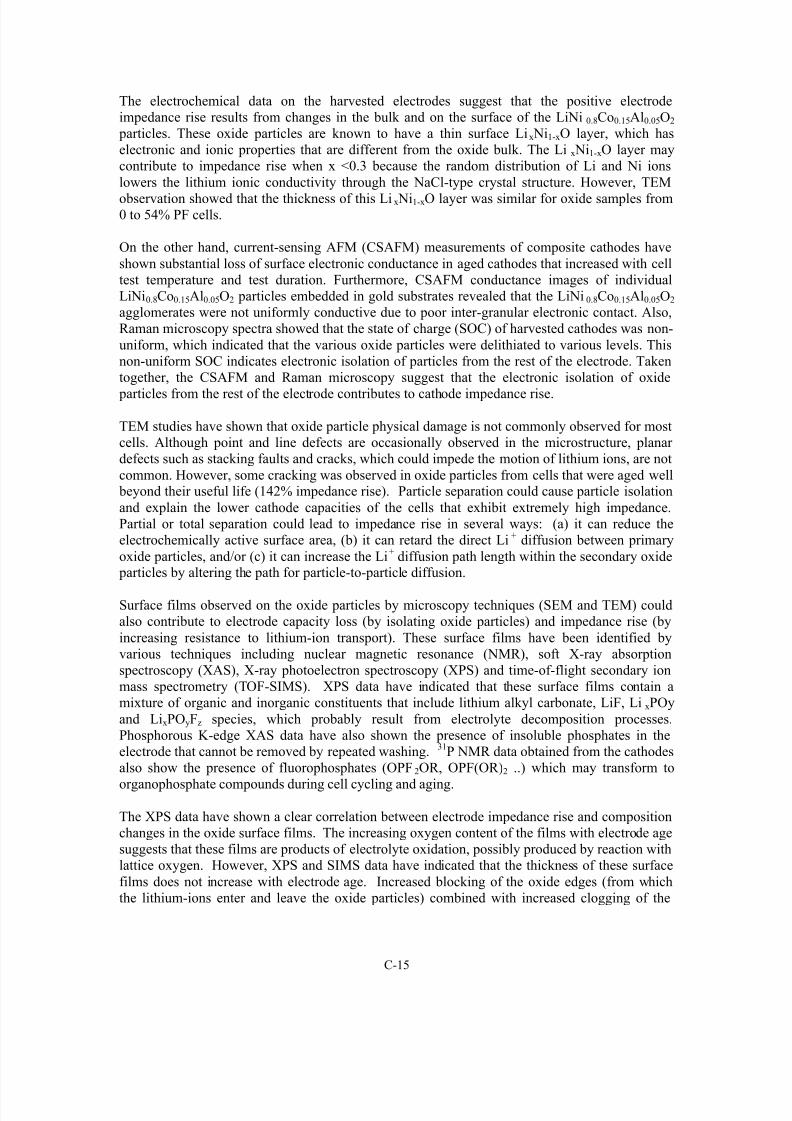
8/11/2019 Battery Life Verification Test Manual
http://slidepdf.com/reader/full/battery-life-verification-test-manual 109/133
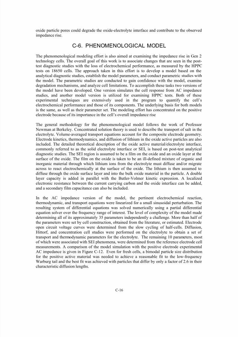
8/11/2019 Battery Life Verification Test Manual
http://slidepdf.com/reader/full/battery-life-verification-test-manual 110/133
C-16
oxide particle pores could degrade the oxide-electrolyte interface and contribute to the observed
impedance rise.
C-6. PHENOMENOLOGICAL MODEL
The phenomenological modeling effort is also aimed at examining the impedance rise in Gen 2
technology cells. The overall goal of this work is to associate changes that are seen in the post-
test diagnostic studies with the loss of electrochemical performance, as measured by the HPPC
tests on 18650 cells. The approach taken in this effort is to develop a model based on the
analytical diagnostic studies, establish the model parameters, and conduct parametric studies with
the model. The parametric studies are conducted to gain confidence with the model, examine
degradation mechanisms, and analyze cell limitations. To accomplish these tasks two versions of
the model have been developed. One version simulates the cell response from AC impedance
studies, and another model version is utilized for examining HPPC tests. Both of these
experimental techniques are extensively used in the program to quantify the cell’s
electrochemical performance and those of its components. The underlying basis for both models
is the same, as well as their parameter set. The modeling effort has concentrated on the positive
electrode because of its importance in the cell’s overall impedance rise
The general methodology for the phenomenological model follows the work of Professor
Newman at Berkeley. Concentrated solution theory is used to describe the transport of salt in the
electrolyte. Volume-averaged transport equations account for the composite electrode geometry.
Electrode kinetics, thermodynamics, and diffusion of lithium in the oxide active particles are also
included. The detailed theoretical description of the oxide active material/electrolyte interface,
commonly referred to as the solid electrolyte interface or SEI, is based on post-test analytical
diagnostic studies. The SEI region is assumed to be a film on the oxide and an oxide layer at the
surface of the oxide. The film on the oxide is taken to be an ill-defined mixture of organic and
inorganic material through which lithium ions from the electrolyte must diffuse and/or migrate
across to react electrochemically at the surface of the oxide. The lithium is then assumed to
diffuse through the oxide surface layer and into the bulk oxide material in the particle. A double
layer capacity is added in parallel with the Butler-Volmer kinetic expression. A localizedelectronic resistance between the current carrying carbon and the oxide interface can be added,
and a secondary film capacitance can also be included.
In the AC impedance version of the model, the pertinent electrochemical reaction,
thermodynamic, and transport equations were linearized for a small sinusoidal perturbation. The
resulting system of differential equations was solved numerically using a partial differential
equation solver over the frequency range of interest. The level of complexity of the model made
determining all of its approximately 35 parameters independently a challenge. More than half of
the parameters were set by cell construction, obtained from the literature, or estimated. Electrode
open circuit voltage curves were determined from the slow cycling of half-cells. Diffusion,
Hittorf, and concentration cell studies were performed on the electrolyte to obtain a set of
transport and thermodynamic parameters for the electrolyte. The remaining 10 parameters, mostof which were associated with SEI phenomena, were determined from the reference electrode cell
measurements. A comparison of the model simulation with the positive electrode experimental
AC impedance is given in Figure C-12. Even for fresh cells, a bimodal particle size distribution
for the positive active material was needed to achieve a reasonable fit to the low-frequency
Warburg tail and the best fit was achieved with particles that differ by only a factor of 2.6 in their
characteristic diffusion lengths.

8/11/2019 Battery Life Verification Test Manual
http://slidepdf.com/reader/full/battery-life-verification-test-manual 111/133
C-17
The HPPC version of the model was utilized primarily to gain confidence in the model and for
cell optimization studies. The parameter set developed for the positive electrode using the AC
impedance version of the model was employed in the HPPC version. HPPC simulations of the
positive electrode compared favorably with experimental tests on reference electrode cells.
Further, parametric studies with the HPPC version of the model suggest that increasing electrode
thickness would improve the initial electrochemical performance, as well as the cell’s aging
characteristics.
EIS studies on the aging of Gen 2 technology cells, described above, indicate that the interfacial
impedance (i.e. the mid-frequency arcs on the Nyquist plot) of the cells grow all through their
life. Furthermore, the low frequency Warburg diffusional impedance tail also begins to increase
late in life. The initiation of the increase in the cell’s diffusional impedance roughly corresponds
to the change in impedance growth rate (i.e. from square-root of time to proportional in time) of
the Gen 2 technology cells as measured by the HPPC tests.
Figure C-12. Comparison between phenomenological model and experiment for the positive
electrode AC impedance (100 kHz-1 mHz) at 60% state-of-charge.
The phenomenological AC impedance model was utilized to examine aging effects associated
with the positive electrode when only its interfacial impedance increases. Three possible sources
for the interfacial impedance increase were identified, which are consistent with experimental
observations. First, an interfacial impedance increase would result from a degradation of the ionic
pathway for lithium ions between the electrolyte in the electrode pores and the bulk oxide activematerial. This could result from changes in the electrolyte/oxide interfacial structure,
composition, and/or properties and would have a direct impact on the positive electrode’s
interfacial impedance. In addition, the size of the model parameter changes needed to account for
the impedance increase suggests that there is a general degradation of the ionic pathway
significantly affecting many of the model’s interfacial parameters. Second, a loss of positive
electrode capacity, particularly isolation of the finer oxide particles would also cause the
interfacial impedance to increase. Simulations based on the measured cell capacity loss suggest
0
5
10
15
20
25
30
0 5 10 15 20 25
Z'(Real) ohm-cm2
- Z " ( I m a g i n a r y ) o h m - c m
2 Experimental
Theoretical

8/11/2019 Battery Life Verification Test Manual
http://slidepdf.com/reader/full/battery-life-verification-test-manual 112/133
C-18
that this effect can at best only be a minor contributor to the positive electrode’s interfacial
impedance increase. Finally, an interfacial impedance increase would result from a degradation of
the electronic pathway between the carbon matrix and the oxide active material, provided that the
carbon matrix has a sufficiently large double layer capacitance associated with it. Degradation of
the electronic pathway is simulated in the model by a large increase in the electronic resistance
between the electronically conducting carbon matrix and oxide active material.
The increase in interfacial impedance of the positive electrode from some combination of the
three mechanisms listed above likely continues throughout the life of the cell. While the model is
able to estimate an upper bounds for the impact of the capacity loss resulting from the isolation of
the oxide active material, the model by itself cannot establish the relative importance of the
changes in the interfacial ionic pathway vs. changes in the interfacial electronic pathway to the
oxide active material. The interfacial ionic pathway tends to be more sensitive to changes in the
interface than the electronic pathway for a wide variety of electrochemical systems, including
many lithium-ion technologies, which suggests that it is most likely to be the primary source of
the impedance increase. Also, it is possible that all three mechanisms are related. As an example,
chemical or physical changes in the SEI could cause degradation of the ionic pathway, as well as
the electronic pathway, at the oxide interface, which could eventually lead to oxide particle
isolation and capacity loss. This type of degradation phenomenon would be consistent with thesquare-root of time impedance growth observed in test cells.
Late in the cell’s life, as the diffusional impedance starts to grow, model simulations indicate that
other positive electrode aging phenomena can contribute to the cell’s impedance rise. These
include a slowing of lithium diffusion within the oxide particles, a loss of electrochemicallyactive area, degradation of electrolyte properties, and a change in electrode microstructure.
Degradation of lithium diffusion through the oxide could be caused from changes in the oxide
structure (e.g. micro-cracks), but also could result from changes in the intra-granular region
between primary particles. A degradation of the intra-granular region and the loss of
electrochemically active area are both consistent with an extensive general degradation of theoxide primary particles’ interfaces. The degradation of electrolyte transport properties and/or a
change in electrode microstructure that increases the electrode’s tortuosity by approximately afactor of 100 can produce an electrode impedance similar to those observed experimentally, but
these degradation mechanisms are not commonly supported by the post-test diagnostic results.
C-7. STATUS SUMMARY
Extensive accelerated aging data were collected on the Gen 2 cells. This appendix reports on the
average values obtained on multiple cells at each test condition and illustrates the differences in
aging characteristics for the Gen 2 baseline and Variant C cells. The only known difference in
these two groups of cells was the level of Al doping in the positive electrode and this apparently
provided some enhanced stability. Although end-of-life for these cells is determined on the basis
of power fade, capacity fade data are included to illustrate the relative ratio of power/capacity
fade for both groups of cells. For a given state of power fade, the Variant C cells exhibited lower capacity fade than the baseline cells.
In the area of accelerated aging, the following insights were gleaned:
• Periodic RPTs were found useful in monitoring changes in the performance
characteristics of the cells as they age:
o EIS was found useful in helping to identify the type of impedance that dominates

8/11/2019 Battery Life Verification Test Manual
http://slidepdf.com/reader/full/battery-life-verification-test-manual 113/133
C-19
o The possibility exists that one or more elements of the RPTs used in this study
contributed in a significant manner to accelerating the aging process(es) and
studies are currently underway to determine the role of some of these elements.
• Aging cells at elevated temperature accelerates the aging process(es) and two or more
different levels of elevated temperature are recommended.
• Aging cells at higher SOC accelerates the aging process(es) and two or more different
levels of SOC are recommended. [Information on this topic is not specifically discussedin this appendix. However, the sensitivity to SOC was obtained in a separate study
conducted by SNL. See reference 21.]
• To a somewhat lesser extent, cycling the cells around a given SOC (vs. non-cycling at the
same SOC) accelerates the aging process(es)
• Several different methods of analyzing the cell aging data were studied and the merits of
each are reported herein.
A considerable amount of diagnostic work, coupled with the phenomenological modeling work,
was performed on cells that incorporate the Gen 2 cell chemistries. The electrochemical
diagnostic studies showed that the major source of impedance rise in these cells was interfacial
impedance at the cathode. Extensive physicochemical diagnostic studies were conducted on all
components of the cells, but for brevity sake this appendix focuses only on the information gainedabout phenomena that could impact on the interfacial impedance of the cathode, via both the
diagnostic studies and the phenomenological modeling work. It should be noted that much care
is needed during the post-test diagnostic studies in order to avoid introducing artifacts associated
with the electrode harvesting and/or sample preparation processes.
In the area of diagnostic studies and phenomenological modeling, the following insights were
gleaned:
•
Removing cells from test at various stages of aging (various levels of power fade) was
useful in that it permitted the periodic characterization and study of individual cell
components at different stages of the aging process.
•
The electrochemical diagnostic studies—using reference electrodes and Li0 counter
electrodes—were extremely beneficial in isolating the major source of cell impedance
rise (interfacial impedance at the cathode), as well as in characterizing the individual
performance capabilities and limitations of anodes and cathodes harvested from new cells
and cells at various stages of aging.
• A large variety of bulk and surface analysis techniques were employed in studying the physicochemical changes that occur in and on the surfaces of the Gen 2 cathodes during
aging. Since the cathodes are non-homogenous composite electrodes that have ~35%
porosity, it is extremely challenging to obtain quantitative information regarding the
observed changes. The techniques discussed in this appendix are the ones that were
found to be the most useful in providing qualitative information about physicochemical
changes associated with the cathodes during aging.
• The phenomenological model was found to be quite useful in conducting parametric
studies of phenomena that could impact on the interfacial impedance of the cathode and
to investigate the magnitude of the individual phenomenon needed to cause the observed
impedance.
o Results suggest that multiple mechanisms—operating simultaneously—are most
probably needed to account for the magnitude of the impedance rise and power
fade observed experimentally.
o The model was able to quantify the possible contribution to impedance rise (and
power fade) associated with particle isolation. The model indicates that this

8/11/2019 Battery Life Verification Test Manual
http://slidepdf.com/reader/full/battery-life-verification-test-manual 114/133
C-20
phenomenon can only be a minor contributor to power fade, based on the ratio of
power/capacity fade observed experimentally for these cells.
The goal of this work was to develop a thorough mechanistic understanding of the factors that
contribute to impedance rise and power fade in these Gen 2 cells. Most, if not all, of the
contributing mechanisms associated with the cathode were identified, however quantifying the
individual contributions of each contributing factor has not yet been achieved. This is extremelychallenging and separate model experiments are currently being used to help develop more
quantitative information on some of the individual contributions. It should be noted that an
essential element of validating any mechanistic model is its ability to correlate degradation rates
to known stress factors, e.g. temperature, SOC, and cycling conditions.

8/11/2019 Battery Life Verification Test Manual
http://slidepdf.com/reader/full/battery-life-verification-test-manual 115/133

8/11/2019 Battery Life Verification Test Manual
http://slidepdf.com/reader/full/battery-life-verification-test-manual 116/133

8/11/2019 Battery Life Verification Test Manual
http://slidepdf.com/reader/full/battery-life-verification-test-manual 117/133
D-3
Appendix D
Use of the Monte Carlo Simulation Tool
D-1. INTRODUCTION
The purpose of the battery life test simulation tool is to aid and support technology life verificationtest (TLVT) planning. The life test simulation tool was implemented using Microsoft Excel and itsintegrated Visual Basic for Applications (VBA) programming language.a The tool as providedimplements the life model found in Section 2.3.1 of the manual, which represents the “true” ASI functionof time as:
)( )
K
K
K ASI ASI 10
1
10
1
1 β
β
β β +
−
−
=
where K = (test time)/(RPT interval), β 0 and β 1 are constant coefficients, and ASI 0 is the true area-specific
impedance at time 0. Provisions are included for the user to modify this model if required.
The tool uses the Monte Carlo approach to add small, random amounts of “noise” to the aboveequation to generate simulated cell ASI data. The “noise” comes from variations in the cell-to-cell ohmicresistance, active area, and measurement errors. The simulated ASI data from one or more cells are thenstatistically analyzed using a robust orthogonal regression (ROR) method to approximate the values of β 0, β 1 and ASI 0. (Reference 4)
The same statistical analysis can be used on data from actual cell tests. Values of ASI 0 and life ontest are calculated from the data. The analysis of experimental data also includes bootstrap analysis, usedto estimate the lower 90% confidence interval in the life on test (see Reference 7).
D-2. START-UPWhen started, the workbook has four worksheets containing the input data, intermediate results,
and final results. These sheets are called Test Data, Life Projection, Experimental Data, and Seedsrespectively. They should not be altered or removed by the user. b
Select the “Test Data” sheet by clicking on its tab. A display similar to that shown in Figure D-1will be seen. Here, values of various parameters can be seen along with some values of the calculatedASI. Execution of the tool is started by left-clicking on the square labeled “MCS.”
a. The tool is contained in Excel spreadsheet file “ Battery MCS.ver.4b.XLS.” Computer system requirements to use the tool areone of the following: ( PC ) Office97 or later installed, Office2000 or later preferred; WP Drawing Characters font installed withinExcel. ( Mac) OS9 with Office2001.
b. If the tool finds a sheet missing, a fatal error will be generated, telling the user which sheet is missing. The user may add anew sheet and rename it appropriately, although some of the text in the cells may be missing if this is done. It is preferable torevert to a saved copy of the tool to avoid user-introduced errors.
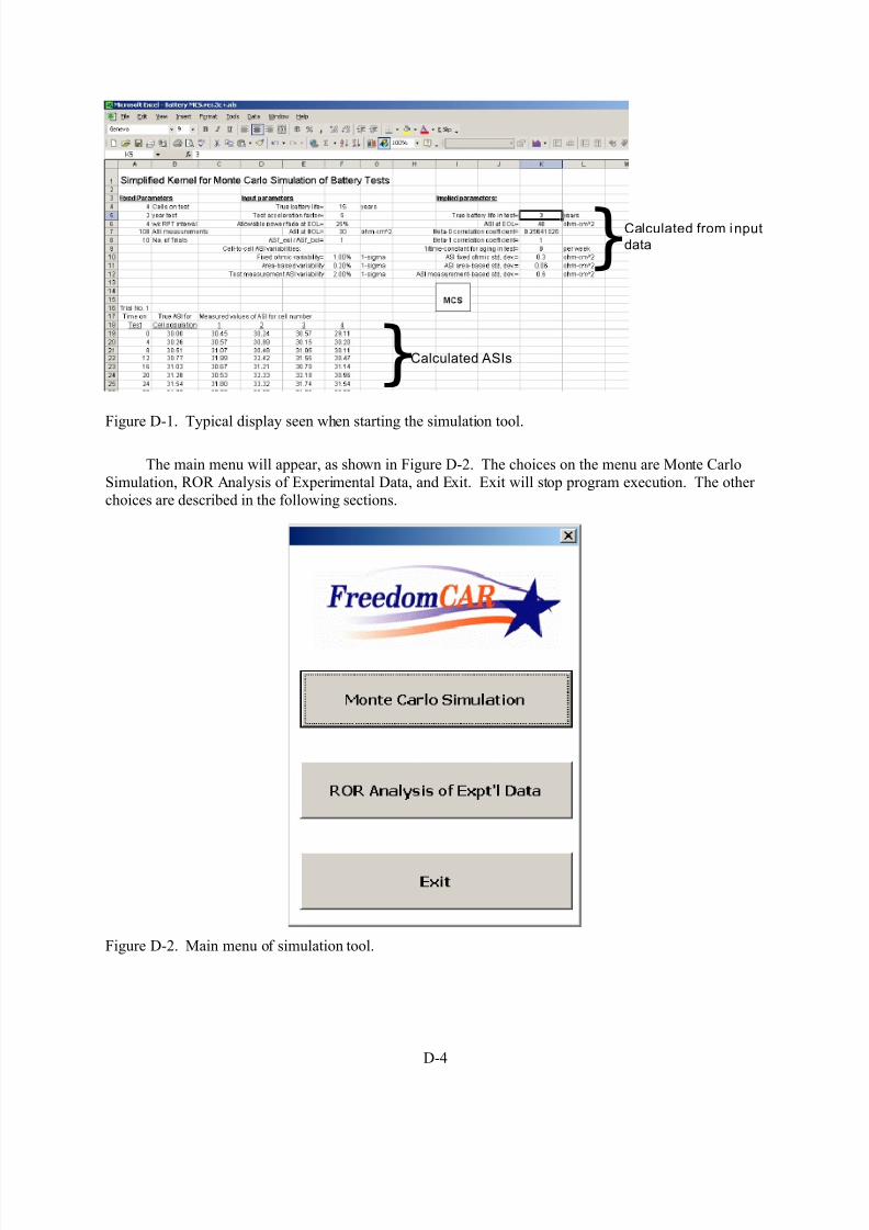
8/11/2019 Battery Life Verification Test Manual
http://slidepdf.com/reader/full/battery-life-verification-test-manual 118/133

8/11/2019 Battery Life Verification Test Manual
http://slidepdf.com/reader/full/battery-life-verification-test-manual 119/133
D-5
D-3. MONTE CARLO SIMULATION
D-3.1 Descr iption of Menu Choices
Clicking on the Monte Carlo Simulation button will bring up a second menu with four options, as
shown in Figure D-3 and described below.
Figure D-3. Monte Carlo menu.
Use New Data In Simulation. This choice is used for starting a completely new simulation. Thedisplay shown is very similar to that shown in Figure D-4, except that all input values are initially set tozero and must be entered by the user. See “Edit Previous Data” for more details.
Figure D-4. Edit data display.
Edit Previous Data for Simulation. This choice is used for starting a new simulation whileretaining some or all of the inputs for the previous run. A display similar to Figure D-4 is shown,allowing the user to change any of the values in the white boxes, which are the parameters that control the

8/11/2019 Battery Life Verification Test Manual
http://slidepdf.com/reader/full/battery-life-verification-test-manual 120/133
D-6
simulation behavior. The user can also turn on or off some error messages by clicking on the “Error Messages On?” box. A complete list of these error messages is given under “Error Messages On?” (SeeSection D-3.3 for more information.)
The ratio (ASI’ at EOL / ASI’ at BOL) has a profound effect on the shape of the ASItrue versus timecurve. See Section 2.1 of the manual for information on this parameter.
The values marked “Tuning constants” are used by the ROR analysis. The recommended initialvalue is 6 for both, although values between 2 and 9 are allowable. See Appendix B of the manual for adescription of leveraging and outlier weighting.
Maximum allowable values for other parameters are given in Table D-1. Additionally, the lengthof the test (in weeks, where a year equals 52 weeks) must be evenly divisible by the RPT interval (inweeks).
Table D-1. Maxima for some of the values used in the simulation calculation.
Parameter Maximum Value
Number of cells 250
Length of test, number of trials, RPT Interval (No. of trials × test length × 52) / (RPT interval) +(No. of trials) × 3 + 18 ≤ 65000
Allowable power fade 25%
Tuning constants >2 and <9
All inputs are checked for validity. Negative number inputs are not valid. Invalid inputs willgenerate an error message, such as “RPT interval: RPT interval=0!” if the RPT interval were mistakenlyset to zero. Click “GO” to start the calculation or “Cancel” to go back to the previous menu.
Recycle/Edit Simulation. This choice is used for making repeated runs with a fixed cell population.
It reuses the data from the most recent simulation run, which is stored in the Seeds spreadsheet. A displaysimilar to Figure D-4 is shown, except that the values that affect cell population size, test length, etc.,cannot be changed. The parameters that can be changed are shown in white boxes and consist of allowable power fade, ASI at BOL, ASI’ at EOL / ASI’ at BOL, and the percent cell-to-cell variabilities(ohmic, area, and measurement).
Error messages can be turned on or off, and inputs are checked for validity, as described in the“Edit Previous Data” case. Click “GO” to start the calculation or “Cancel” to go back to the previousmenu.
Exit. This choice returns to the previous menu.
D-3.2 Normal Operation
The calculation will start after clicking “GO.” If Excel97 or Excel for Office2001 is running,Excel will disappear until the calculation is complete or an error is encountered (depending on the statusof “Error Messages On?”). With more recent versions of Excel, a progress bar will appear, as shown in

8/11/2019 Battery Life Verification Test Manual
http://slidepdf.com/reader/full/battery-life-verification-test-manual 121/133
D-7
Figure D-5, displaying the actual number of trials as well as the percentage of completion based on theinput number of trials.c
50%
Calculation in Progress
10Number of Trials
50%
Calculation in Progress
10Number of Trials
Figure D-5. Progress bar showing status of calculation in Excel XP.
Assuming that the run was successful, a display similar to that given in Figure D-6 will be shownto the user. The display summarizes all the input data and shows the results of the life projections. T -statistics are used to estimate the upper and lower limits for the 90% confidence interval. Of interest isthe estimated minimum life with 90% confidence, shown in the boxed area.
Figure D-6. Results of a simulation calculation.
Clicking on “Save Results” will allow the user to save the current life projection results for later use. Clicking here produces the dialog box shown in Figure D-7. The user is asked to enter a valid sheetname (length of name < 32 characters). If the sheet name already exists, the user will be prompted to tryanother name. Clicking “OK” copies the contents of the Life Projection sheet to a new sheet and renamesthat new sheet to whatever the user entered.d The user is taken to the menu shown in Figure D-3 when thedesired operation is complete. Clicking on “Cancel” aborts the operation and returns the user to thedisplay shown in Figure D-6.
c. This display will only be seen if the “WP Box Drawing” font set is installed in Excel. Otherwise a dollar sign, ‘$’, will appear.
d. The user is cautioned not to add too many worksheets. The maximum number of worksheets is limited by available computer resources (not checked by the tool). Adding many worksheets slows loading and saving of the tool and results.
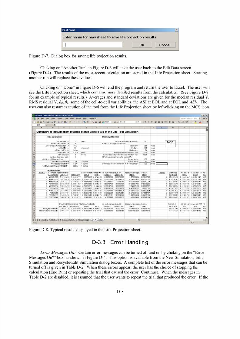
8/11/2019 Battery Life Verification Test Manual
http://slidepdf.com/reader/full/battery-life-verification-test-manual 122/133

8/11/2019 Battery Life Verification Test Manual
http://slidepdf.com/reader/full/battery-life-verification-test-manual 123/133
D-9
error is repeatedly produced due to the random numbers being used in the simulation, the user has to waituntil either better-behaved results are obtained or a runaway calculation is detected, as described below.
Table D-2. List of error messages.
Bad values in estimation of ASIo!
Poorly-behaved FittedBeta1 found! Trial # x will repeat.
FittedBeta0 + (FittedBeta1 - 1) * ASIo <= 0! Trial # x will repeat.
FittedBeta0 + 1 /(1-AllowablePFade) * (FittedBeta1-1) * ASIo <= 0! Trial # x will repeat.
[FittedBeta0+(1/1-AllowablePFade)*(FittedBeta1-1) *ASIo]/[FittedBeta0+(FittedBeta1-1)*ASIo]<= 0! Trial # x will repeat.
If the “Error Messages On?” box is checked, error messages will be shown when certain criteria aremet, such as β 1=1. In the case of β 1=1, the second message in Table D-2 will be shown. The user is thengiven the chance to stop the entire calculation or repeat the trial.
If a runaway calculation is found, an error message stating “Bad input data!” will be generated, andthe run will end. A runaway calculation is defined as the actual number of trials exceeding the requestednumber by 20.
D-4. ROR ANALYSIS OF EXPERIMENTAL DATA
In addition to simulating cell performance data, the tool can import and analyze actual cell data.Clicking on the ROR Analysis of Experimental Data button on the main menu (Figure D-2) produces thedialog box shown in Figure D-9. It is assumed that the data to be imported are in an Excel workbook andform a contiguous block. Data import will stop where empty cells are encountered.
The information needed to read the data is specified in the dialog box, which is illustrated with
typical values in Figure D-9. This information includes the complete path to the workbook and its filename (drive:\directory\filename.ext), the worksheet name that contains the cell data, the number of actualcells tested, the maximum number of RPTs per cell in the file, the starting location of the cell data, theRPT interval, the allowable power fade for life on test estimation (maximum of 25%), tuning constantsfor leverage and outlier weights (see the “Edit Previous Data” section for more details), and the dataorientation on the worksheet.
The worksheet name is case sensitive; other inputs are not. They are retained while the program isrunning. If ROR Analysis is used more than once while the program is running, they will appear again.This is used when multiple analyses of data are done from the same source or when the path and/or sheetnames for different workbooks differ only slightly.
For the “maximum number of RPTs,” the RPT count starts at 0 weeks and ends with the last RPTfrom the longest-lived cell in the dataset. For example, if all cells last 104 weeks and the RPT interval is4 weeks, the maximum number of RPTs per cell in file is 27. This is true even if some cells do notcontinue for the full 104-week duration.

8/11/2019 Battery Life Verification Test Manual
http://slidepdf.com/reader/full/battery-life-verification-test-manual 124/133
D-10
Figure D-9. Dialog box for importing experimental data from Excel for analysis.
Data orientation refers to the direction of increasing time in the worksheet. An example of verticalorientation is given in Figure D-10, and horizontal in Figure D-11. In Figure D-10, time increases down acolumn, e.g., 0 weeks in cell A2, 4 weeks in A3, 8 weeks in A5, etc. In Figure D-11, time increasesacross a row, e.g., 0 weeks in B1, 4 weeks in C1, 8 weeks in D1, etc. For these examples, both blocks of ASI data begin at cell B2. The user indicates the orientation of the data by clicking on the icons next tothe “Data Orientation in Spread Sheet” label. The program will indicate the user’s selection by changingthe selected icon to white and the icon not selected to gray. In Figure D-9, the vertical data orientation isselected.
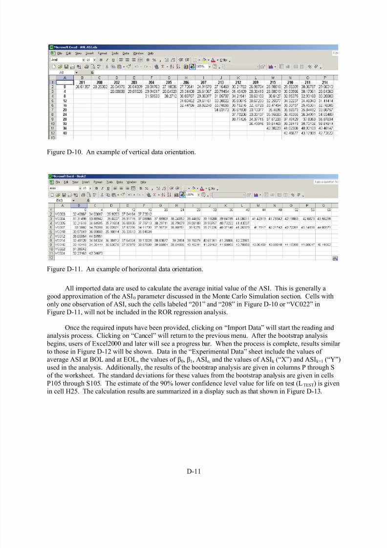
8/11/2019 Battery Life Verification Test Manual
http://slidepdf.com/reader/full/battery-life-verification-test-manual 125/133
D-11
Figure D-10. An example of vertical data orientation.
Figure D-11. An example of horizontal data orientation.
All imported data are used to calculate the average initial value of the ASI. This is generally agood approximation of the ASI0 parameter discussed in the Monte Carlo Simulation section. Cells withonly one observation of ASI, such the cells labeled “201” and “208” in Figure D-10 or “VC022” inFigure D-11, will not be included in the ROR regression analysis.
Once the required inputs have been provided, clicking on “Import Data” will start the reading andanalysis process. Clicking on “Cancel” will return to the previous menu. After the bootstrap analysis begins, users of Excel2000 and later will see a progress bar. When the process is complete, results similar to those in Figure D-12 will be shown. Data in the “Experimental Data” sheet include the values of average ASI at BOL and at EOL, the values of β0, β1, ASIo, and the values of ASIk (“X”) and ASIk+1 (“Y”)used in the analysis. Additionally, the results of the bootstrap analysis are given in columns P through Sof the worksheet. The standard deviations for these values from the bootstrap analysis are given in cells
P105 through S105. The estimate of the 90% lower confidence level value for life on test (LTEST) is givenin cell H25. The calculation results are summarized in a display such as that shown in Figure D-13.

8/11/2019 Battery Life Verification Test Manual
http://slidepdf.com/reader/full/battery-life-verification-test-manual 126/133
D-12
Figure D-12. Example results from the Import Data function.
Figure D-13. Display showing results from ROR and bootstrap analysis on experimental data.
8/11/2019 Battery Life Verification Test Manual
http://slidepdf.com/reader/full/battery-life-verification-test-manual 127/133
D-13
D-5. USER LIFE EQUATIONS
The tool has provisions for use with technology-dependent life equations, which can be substitutedfor the default ones described in this manual. These technology-dependent computer routines are storedin a single VBA module.e The following discussion assumes some familiarity with VBA.
Double-clicking on the Modules icon in the window labeled “Project-VBAProject” will displaytwo user-modifiable modules, called MakeVisible and UserEquations. The MakeVisible module(accessed by double-clicking on its icon) contains a single subroutine, to be used only when needed due to premature termination of the program, as might occur with a poorly handled error condition.
The UserEquations module contains three functions: LifeEquation, EstimateASI_at_EOT, andEstimateLife. The function names and variables in the function headers cannot be changed withoutimpairing the operation of the tool. The three functions contain some internal documentation thatdescribes their internal variables. This information may provide some guidance in constructingreplacement functions. The user is warned that error detection and trapping is necessary when these
modules are modified. Aberrant behavior is likely to occur without it. The nature and extent of error detection and trapping to be provided is left to the user.
LifeEquation . Test time in weeks is passed to the function. Based on the true values of beta0 andbeta1, the function will return the true value of ASI. If the user changes this function, error trapping akinto that shown below is needed. The case where beta1=1 for the default life function is illustrated here.
' VARIABLES:
' beta0 value of beta0 based on initial "true" conditions (passed globally)' beta1 value of beta1 based on initial "true" conditions (passed globally)' ASI_at_BOL true value of ASI at time=0 (passed globally)' T time on test, in weeks' RecipTimeConstant ln(beta1) / RPTInterval'
If beta1 = 1 Then a = ASI_at_BOL + beta0 * T / RPTInterval Else a = ((beta0 + (beta1 - 1) * ASI_at_BOL) * Exp(T *
RecipTimeConstant) - beta0) / (beta1 - 1)End If
The condition beta1=1 would produce a divide by zero error if it were not trapped by the If statement.
EstimateASI_at_EOT. This boolean function contains the life equation and is passed threevariables: WhichCase, fbeta0, and fbeta1. It returns the estimated ASI at end of test, ASIest, as well as
status (see below for more information). The function header is given below. If the user modifies thisfunction, function status must be returned or the rest of the analysis may not work. If EstimateASI_at_EOT equals true, it means a successful calculation with no errors.
e Windows users can access the VBA development environment using Ctrl+F11 keystrokes. (Option+F11 for Mac users.)The description here is based on the Windows version of Excel, although the Macintosh environment is similar.

8/11/2019 Battery Life Verification Test Manual
http://slidepdf.com/reader/full/battery-life-verification-test-manual 128/133
D-14
' VARIABLES
' Whichcase = used for program run control. Do not change' fbeta0 = fitted beta0; passed to function by value. Do not change in header ' fbeta1 = fitted beta1; passed to function by value. Do not change in header ' ASIest = returned value of estimated ASI
' RealBatteryLife = true battery life; passed globally' AcceleratingFactor = stress level or acceleration factor; passed globally' RPTInterval = time between RPTs; passed globally' EMsgsOn = boolean set by the user on new, edit or recycle simulation' MCSMsgBox = simple control to either terminate or continue program based on user
selection
Function EstimateASI_at_EOT(ByRef WhichCase As Integer, ByVal fbeta0 As Double, ByValfbeta1 As Double, ByRef ASIest As Double) As Boolean
The user is responsible for providing error trapping. (See the VBA code in the UserEquationsmodule for examples.)
EstimateLife. This boolean function is the life equation solved for time in terms of beta0, beta1,and ASIo. It is passed three values, WhichCase, fbeta0, and fbeta1, and it returns the estimate of life ontest, Life_est, as well as status (see below for more information). The function header is given below. If the user modifies this function, function status must be returned or the rest of the analysis may not work.If EstimateLife equals true, it means a successful calculation with no errors.k
' VARIABLES
' Whichcase = used for program run control. Do not change' fbeta0 = fitted beta0; passed to function by value. Do not change in header ' fbeta1 = fitted beta1; passed to function by value. Do not change in header ' Life_est = returned value of estimated life in test
' AllowablePfade = allowable power fade; passed globally' ASIo = estimate of ASIo; passed globally' RPTInterval = time between RPTs; passed globally
Function EstimateLife(ByRef WhichCase As Integer, ByVal fbeta0 As Double, ByVal fbeta1 AsDouble, ByRef Life_est As Double) As Boolean
The user is responsible for providing error trapping. (See the VBA code in the UserEquationsmodule for examples.)
8/11/2019 Battery Life Verification Test Manual
http://slidepdf.com/reader/full/battery-life-verification-test-manual 129/133
E-1
Appendix E
Test Measurement Requirements

8/11/2019 Battery Life Verification Test Manual
http://slidepdf.com/reader/full/battery-life-verification-test-manual 130/133
E-2

8/11/2019 Battery Life Verification Test Manual
http://slidepdf.com/reader/full/battery-life-verification-test-manual 131/133
E-3
Appendix E
Test Measurement Requirements
The important measurement parameters for life testing are current, voltage, and temperature (and,
implicitly time). All other reported parameters are derived (e.g., charge and energy) or calculated (e.g.,resistance, pulse power capability, etc.) from voltage and current measurements, and the test temperature
also affects many of the parameters when measurements are taken.
E-1. ELECTRICAL PARAMETERS
For life testing and life prediction purposes, the critical aspects of current and voltage
measurements are (a) linearity and (b) test-to-test repeatability (i.e., stability). Absolute accuracy of
electrical measurements is important for some calculated parameters, but the simplest parameter used for
life prediction [resistance, or equivalently ASI (area-specific impedance)] is computed using a ∆V/∆I
formula whose results for a single test are affected only by random errors or calibration linearity errors in
voltage or current.
The relationship between current and voltage errors and the resulting uncertainty in calculated
pulse resistance is detailed in Reference 22, Volume 1, Section 3.2.4. Voltage and current calibration
errors are directly additive (in an RMS sense), while random measurement errors are “amplified”
according to the fraction of the measurement range used to measure ∆V or ∆I. Thus, the uncertainty in
resistance is data-dependent; but a high-quality measurement system using 16-bit data acquisition and
precision current shunts (if properly calibrated) should yield data adequate to calculate resistance with anuncertainty of 0.5% or less for a single measurement. For example, Reference 22, Volume 2, shows the
calculated resistance uncertainty (one standard deviation) for a Maccor battery tester (claimed voltage and
current repeatability of 0.02% of full scale) to be less than 0.4% of reading, even when ∆V and ∆I were
only 5 and 8% of full scale, respectively. (A majority of this uncertainty was due to the 0.25% current
shunts used for calibration at the time this report was written.)
Note that computing pulse resistance and other dynamic battery characteristics in this fashion
requires paired current and voltage measurements that are essentially simultaneous in time (i.e., acquired
within <0.01s of each other). A significant time skew between current and voltage measurements will
create device-dependent errors in the calculated results that cannot be compensated for and are not
accounted for in the uncertainty values described above.
Test-to-test repeatability may involve additional errors that affect this result. Only a limited study
of the effect of voltage or current calibration drift in actual testing has been made. However, as long as
drift effects are contained within the calibration uncertainty specifications, they should not affect this
result substantially.
To ensure that resistance can be determined with an uncertainty of 0.5% or less, the following
specifications can be used as a guideline:a
• Voltage calibration uncertainty <0.1% of full scale
a. There are two important caveats on these specifications. (1) These values are based on a one-standard-deviation uncertainty
for resistance. Raising the confidence level substantially (e.g., to two standard deviations) while maintaining a 0.5% limit is possible but probably near the limit of present measurement capabilities in any known battery-testing laboratory. (2) The higher
allowable errors for current measurements are due to the likelihood that ∆V measurements will use a smaller fraction of themeasurement range than the corresponding current measurements.

8/11/2019 Battery Life Verification Test Manual
http://slidepdf.com/reader/full/battery-life-verification-test-manual 132/133
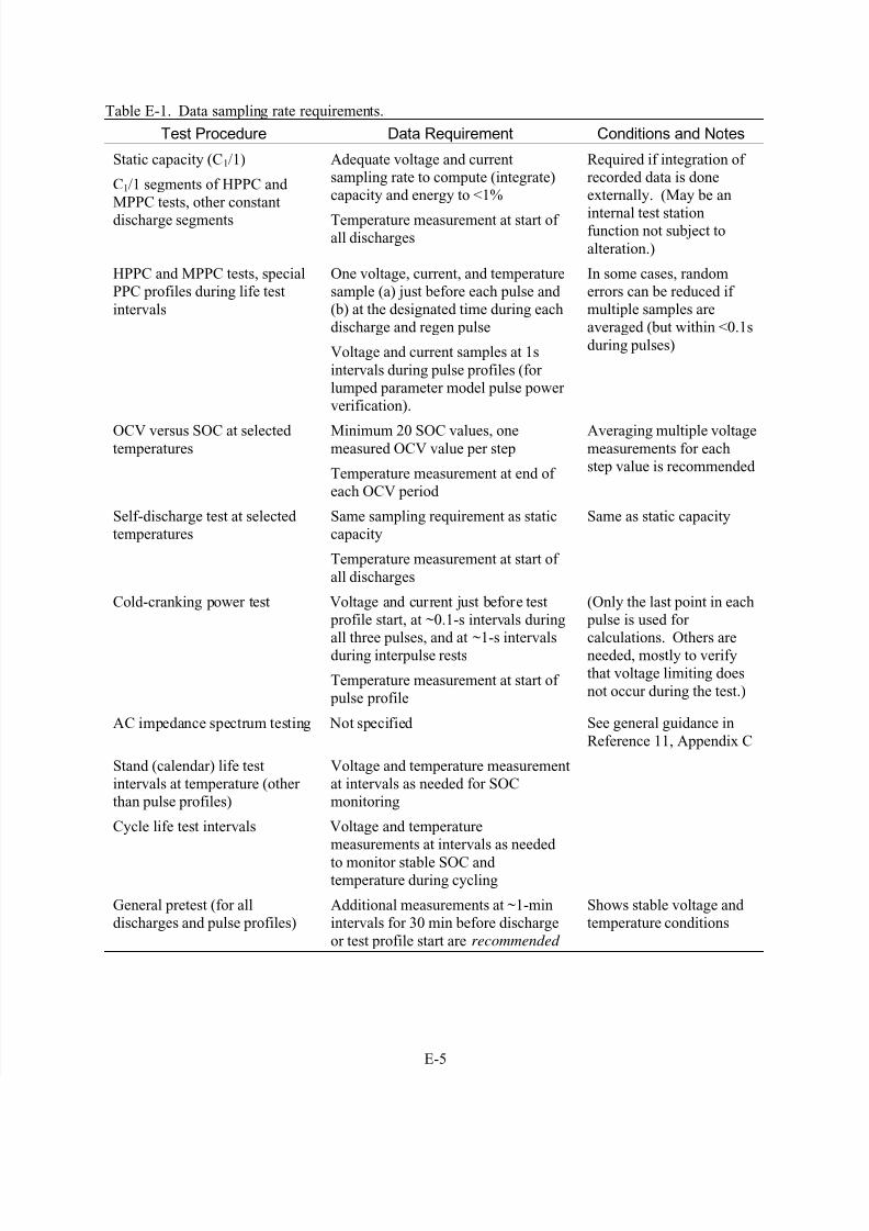
8/11/2019 Battery Life Verification Test Manual
http://slidepdf.com/reader/full/battery-life-verification-test-manual 133/133
Table E-1. Data sampling rate requirements.
Test Procedure Data Requirement Conditions and Notes
Static capacity (C1/1)
C1/1 segments of HPPC and
MPPC tests, other constant
discharge segments
Adequate voltage and current
sampling rate to compute (integrate)
capacity and energy to <1%
Temperature measurement at start of all discharges
Required if integration of
recorded data is done
externally. (May be an
internal test stationfunction not subject to
alteration.)
HPPC and MPPC tests, special
PPC profiles during life test
intervals
One voltage, current, and temperature
sample (a) just before each pulse and
(b) at the designated time during each
discharge and regen pulse
Voltage and current samples at 1s
intervals during pulse profiles (for
lumped parameter model pulse power
verification).
In some cases, random
errors can be reduced if
multiple samples are
averaged (but within <0.1s
during pulses)
OCV versus SOC at selected temperatures
Minimum 20 SOC values, onemeasured OCV value per step
Temperature measurement at end of
each OCV period
Averaging multiple voltagemeasurements for each
step value is recommended
Self-discharge test at selected
temperatures
Same sampling requirement as static
capacity
Temperature measurement at start of
all discharges
Same as static capacity
Cold-cranking power test Voltage and current just before test
profile start, at ~0.1-s intervals during
all three pulses, and at ~1-s intervals
during interpulse rests
(Only the last point in each
pulse is used for
calculations. Others are
needed mostly to verify