
Battelle Team Dose Reconstruction Project for NIOSH Team Dose Reconstruction Project for NIOSH...
70
Battelle Team Dose Reconstruction Project for NIOSH Document Title: Default Assumptions and Methods for Atomic Weapons Employer Dose Reconstructions Document Number: Battelle-TIB-5000 PNWD-3741 Revision: 00 Effective Date: 02 Apr. 2007 Type of Document: Technical Information Bulletin (TIB) Supersedes: None Subject Experts: Daniel J. Strom Document Owner Approval: Signature on file Approval Date: 20 Dec 2006 Daniel J. Strom, Staff Scientist Approval: Signature on file Approval Date: 20 Dec 2006 Jay A. MacLellan, Battelle PNWD Task Manager Concurrence: Signature on file Concurrence Date: 20 Dec 2006 Richard J. Traub, Staff Scientist Approval: Signature on file Approval Date: 02 Apr 2007 James W. Neton, Associate Director of Science New Total Rewrite Revision Page Change FOR DOCUMENTS MARKED AS A TOTAL REWRITE, REVISION, OR PAGE CHANGE, REPLACE THE PRIOR REVISION AND DISCARD / DESTROY ALL COPIES OF THE PRIOR REVISION.
Transcript of Battelle Team Dose Reconstruction Project for NIOSH Team Dose Reconstruction Project for NIOSH...

Battelle Team Dose Reconstruction Project for NIOSH
Document Title: Default Assumptions and Methods for Atomic Weapons Employer Dose Reconstructions
Document Number: Battelle-TIB-5000 PNWD-3741
Revision: 00
Effective Date: 02 Apr. 2007
Type of Document: Technical Information Bulletin (TIB)
Supersedes: None
Subject Experts: Daniel J. Strom
Document Owner Approval:
Signature on file Approval Date: 20 Dec 2006
Daniel J. Strom, Staff Scientist
Approval: Signature on file Approval Date: 20 Dec 2006 Jay A. MacLellan, Battelle PNWD Task Manager
Concurrence: Signature on file Concurrence Date: 20 Dec 2006 Richard J. Traub, Staff Scientist
Approval: Signature on file Approval Date: 02 Apr 2007 James W. Neton, Associate Director of Science
New Total Rewrite Revision Page Change FOR DOCUMENTS MARKED AS A TOTAL REWRITE, REVISION, OR PAGE CHANGE, REPLACE THE PRIOR
REVISION AND DISCARD / DESTROY ALL COPIES OF THE PRIOR REVISION.

Document No. Battelle-TIB-5000 PNWD-3741
Revision No. 00 Effective Date: 04/02/2007 Page iii
Publication Record
EFFECTIVE DATE
REVISION NUMBER DESCRIPTION
27 March 2006 00 - A Document initiated by Daniel J. Strom 4 April 2006 00 – A.01 Corrections to Eisenbud 1950 data, other errors; revision of 3.0 24-28 April 06 00 – A.02 Additions May 2006 00 – A.03 Additions May 2006 00 – A.04 Additions May 2006 00 – A.06 Additions July 2006 00 – A.07 Added 3.17 31 July 2006 00 – A.10 Review draft sent to NIOSH 11 Sept 2006 00 – A.11 Response to NIOSH Comments
Radon and Thoron section completed Added Section 3.23, Use of time-dependent data
21 Sept 2006 00 – A.12 Fixed List of Tables 13 Oct 2006 00 – A.13 Responding to comments from OCAS 7 Nov 2006 00 – E.01 Completed comment responses to OCAS 20 Dec 2006 00 – F Completed comment responses to OGC
Document No. Battelle-TIB-5000 PNWD-3741
Revision No. 00 Effective Date: 04/02/2007 Page iv
Contents
Publication Record....................................................................................................................................... iii Acronyms and Abbreviations ....................................................................................................................viii 1.0 Introduction ...................................................................................................................................... 10 2.0 Fitting Statistical Distributions to Data ............................................................................................ 11
2.1 Lognormal Distributions ......................................................................................................... 11 2.1.1 Uncensored Individual Observations ......................................................................... 12 2.1.2 Summary Statistics ..................................................................................................... 13
2.1.2.1 Example Using Two Data Points ............................................................... 14 2.1.2.2 Using Minimum, Mean, and Maximum Values with Number of
Observations to Determine the Parameters of a Lognormal Distribution.. 15 2.1.2.3 Using Range and Mean Value without Number of Observations to
Determine the Parameters of a Lognormal Distribution ............................ 15 2.1.2.4 Use of Range and Average Value Data that Are Inconsistent with a
Lognormal Distribution ............................................................................. 16 2.1.2.5 Use of a Single Measurement Value.......................................................... 17
2.1.3 Censored Individual Observations ............................................................................. 17 2.1.3.1 Left-Censored Data .................................................................................... 17 2.1.3.2 Finney Weighting Factors.......................................................................... 18 2.1.3.3 Right-censored Data................................................................................... 19
2.1.4 Grouped, Censored Observations............................................................................... 19 2.1.4.1 Frequency Weighting for Grouped Data.................................................... 20
2.1.5 “Reasonableness” of a Lognormal Distribution ......................................................... 22 2.1.6 Summary of Default Assumptions for Fitting Lognormal Distributions ................... 23
2.2 Triangular Distributions .......................................................................................................... 23 2.3 Normal Distributions............................................................................................................... 26
2.3.1 Normally-distributed Measurement Uncertainty and an Underlying Lognormally-distributed Measurand: Mirror Image Method ........................................................... 26
2.3.2 Normally-distributed Measurement Uncertainty and an Underlying Lognormally-distributed Measurand: Preserved Mean and Variance Method................................. 27 2.3.2.1 Test of the Preserved Mean and Variance Method .................................... 28
2.4 Rectangular Distributions........................................................................................................ 32 2.5 Constant “Distributions” ......................................................................................................... 32
3.0 Default Assumptions ........................................................................................................................ 33 3.1 Introduction ............................................................................................................................. 33 3.2 External Irradiation Geometry................................................................................................. 33 3.3 The 95%ile and “Constant” Uncertainty Distribution for Limited Data Sets ......................... 34 3.4 Uncertainty in Biokinetic Models ........................................................................................... 34 3.5 Aerosol Particle Size and Respirable Fraction ........................................................................ 35
Document No. Battelle-TIB-5000 PNWD-3741
Revision No. 00 Effective Date: 04/02/2007 Page v
3.6 Use of Time-period-specific, Process-based GSDs for Published Mean Aerosol
Concentration Data.................................................................................................................. 36 3.7 Use of Distributions to Describe Multiple Populations........................................................... 37 3.8 Use of Time-Weighted Averages, Breathing Zone (BZ) Air Samples, and General Area
(GA) Air Samples, Process (P) Air Samples, and Considerations of Sample Duration.......... 38 3.9 Particle Solubility (ICRP 66 Transportability Classes F, M, S) and f1 (Gastrointestinal
Absorption Fractions).............................................................................................................. 41 3.10 Exposure Time and Intake Calculations.................................................................................. 42 3.11 Ingestion .................................................................................................................................. 42 3.12 Occupational Medical Doses................................................................................................... 42 3.13 External Dose Conversion Factors .......................................................................................... 43 3.14 External Missed Dose When There Was Monitoring.............................................................. 43 3.15 Internal Missed Dose When There Was Monitoring............................................................... 43 3.16 Environmental Dose ................................................................................................................ 43 3.17 Radon and Thoron and Their Short-lived Decay Products...................................................... 43
3.17.1 Radon and Thoron...................................................................................................... 44 3.17.2 Potential Alpha Energy Exposure and Concentration ................................................ 44 3.17.3 Equilibrium Factors.................................................................................................... 45 3.17.4 Summary of radon and thoron quantities and conversion factors .............................. 47
3.18 Radium Monitoring by Breath Radon Analysis ...................................................................... 48 3.19 Determination of the Uncertainty Distribution for Annual Organ Doses Summed Over
Multiple Intakes....................................................................................................................... 48 3.20 Representativeness of Air Samples ......................................................................................... 52
3.20.1 Inferring Representativeness by Comparing BZ with GA Samples........................... 52 3.20.2 Inferring Representativeness by Comparing Excretion Rates Predicted from Air
Samples with Measured Excretion Rates .................................................................. 55 3.21 Propagation of Medians and Uncertainties for Lognormal Distributions ............................... 56
3.21.1 Propagation of Medians (not Means) for Products of Lognormal Distributions........ 56 3.21.2 Propagation of Uncertainties for Lognormal Distributions........................................ 57
3.22 Adding Doses with Differing Distributions ............................................................................ 57 3.23 Adjusting Process-Specific Dose Rates or Air Concentrations for Time Trends over
Periods of Years ...................................................................................................................... 58 4.0 Glossary............................................................................................................................................ 63 5.0 References ........................................................................................................................................ 67
Document No. Battelle-TIB-5000 PNWD-3741
Revision No. 00 Effective Date: 04/02/2007 Page vi
Figures
Figure 1. Finney weights (y), standard normal distribution, and ratio. 18 Figure 2. Lognormal fits to 194 air monitoring results from one site, with the first 39 results being 0 or “less-thans”. 19 Figure 3. Examples of fitting a lognormal distribution to grouped, left- and right-censored data (from Table 7, 1949, Eisenbud and Quigley 1956) 20 Figure 4. Mean, median, and upper 95th %ile for the airborne uranium data from Table 7 of Eisenbud and Quigley (1956) 21 Figure 5. Lognormal fits to grouped annual deep dose equivalent measurements for 458 persons. Note the significantly different slopes for different weighting. 22 Figure 6. The probability density function (pdf), cumulative density function (cdf), and parameters of a triangular distribution 24 Figure 7. Analysis of Y-12 uranium in urine measurements (Strom 1984, Figure 16). a. the product of a lognormal and a normal distribution producing a negative tail. b. histogram of uranium excretion values from Y-12 in 1971. 27 Figure 8. Normalized probability density functions (pdfs) for Hanford in vivo 137Cs measurements on unexposed workers 29 Figure 9. Cumulative probability density functions (cdfs), observed (rough red line) and predicted (smooth line) using GSD = 1.4 29 Figure 10. PDFs with uncertainty model (smooth thin line), lognormal "true state of nature" model (dashed line), and predicted value (heavy black line) 31 Figure 11. Residuals for predicted cdf. 31 Figure 12. Lognormal plot of mean airborne U concentrations for 136 different processes in uranium refining (Christofano and Harris 1960). 37 Figure 13. Time-Weighted Average (TWA) Radon Concentration in Air, WL (if 100% equilibrium) 40 Figure 14. Distribution of results from Monte Carlo simulation of TWA radon data. 41 Figure 15. Graph of 10,000 Monte Carlo trials adding 10 samples from lognormal distributions with x50 = 1 and GSD = 4. 51 Figure 16. Graph from Caldwell (1972) digitized in Table 3.10. The straight line refers to predictions of the ICRP Publication 2 lung model 53 Figure 17. Comparision of lapel (BZ) air samples to general area air samples (Fig. 4 from Caldwell et al. 1967) 54 Figure 18. Lognormal fit to the ratio of daily uranium excretion divided by the average airborne uranium concentration for maintenance workers, from Yu and Sherwood (1996). 55 Figure 19. Original Figure 1 from Christofano and Harris (1960) showing time-weighted average exposure trends over the years 1948-1956. 58 Figure 20. Analysis of time-weighted average air concentrations from Christofano and Harris (1960; Fig. 1). Variability bars are the geometric mean times or divided by one GSD. 60 Figure 21. Use of year-specific correction factors to adjust air concentrations for processes over time. 61
Tables Table 2.1. Uncertainty distributions and their parameters for input to IREP 11 Table 2.2. Symbols, parameters, and relationships for the lognormal distribution 12 Table 2.3. Fifteen distinct ways of determining a lognormal distribution from minimal information 13 Table 2.4. “Exposure to Soluble Uranium Compounds,” reproduced from Eisenbud and Quigley (1956). 14 Table 2.5. Deriving a lognormal distribution from two data points. 14
Document No. Battelle-TIB-5000 PNWD-3741
Revision No. 00 Effective Date: 04/02/2007 Page vii
Table 2.6. Regression values and statistics for the 1949 example. x , x50, Std. Dev., and Upper 95th %ile are all in mg/m3. 21 Table 2.7. Comparison of attempts to fit lognormal and triangular distributions to mean and range data from Christofano (1960) 25 Table 2.8. 90, 95, and 99 %iles of lognormal "true state of nature" distributions with GSDs of 1.2, 1.4, and 1.6. 32 Table 3.1. Reliability categories for selected results of ICRP Publication 30 biokinetic and dosimetric models 34 Table 3.2. Estimated reliability, for selected radionuclides, of the effective dose coefficient values recommended in ICRP Publication 30 (from NCRP 1998 Table 8.2) 35 Table 3.3. Daily Weighted Rn. Exposure to Tower Workers (Table I from NIOSH Ref ID 8921 p.13, May 1951, Lake Ontario Ordinance Works) 39 Table 3.4. Summary statistics from TWA analysis. 40 Table 3.5. Default exposure time assumptions as a function of date 42 Table 3.6. Uncertainty distributions for equilibrium factors for converting radon and thoron gas measurements to working levels (WL) 47 Table 3.7. Summary of numerical conversions for radon and thoron quantities, regardless of the precision of measurements 48 Table 3.8. Results of adding random samples from 10 lognormal distributions with the same GSD. 50 Table 3.9. Parameters of the lognormal uncertainty distribution due to lack of representativeness of an air sample distribution. 52 Table 3.10. Breathing zone (BZ or Lapel) air sampling and general area (GA) air sampling (data digitized from Caldwell 1972; adapted from (Strom, Watson, and Stansbury 2002)). 53 Table 3.11. Summary statistics for the lognormal fit to the Pu distribution shown in Figure 17. 54 Table 3.12. Results of digitizing data from Figure 19. All concentrations (columns 3-7 and 9) are in dpm/m3 59 Table 3.13. Year-specific correction factors for tabulated process-specific air concentrations, derived from analysis of Christofano and Harris (1960) Fig. 1. 62

Document No. Battelle-TIB-5000 PNWD-3741
Revision No. 00 Effective Date: 04/02/2007 Page viii
Acronyms and Abbreviations
µR microroentgen ABRWH Advisory Board on Radiation and Worker Health AP anterior-posterior AWE Atomic Weapons Employer Bq becquerel BZ breathing zone CATI Computer-Assisted Telephone Interview CV coefficient of variation d/m/m3 disintegrations per minute per cubic meter DCF dose conversion factor DOL Department of Labor dpm disintegrations per minute DR dose reconstruction Dx diagnosis EEOICPA Energy Employees Occupational Illness Compensation Program Act F ICRP Respiratory Tract Transportability Type Fast FGR-12 Federal Guidance Report 12 FUSRAP Formerly Utilized Sites Remedial Action Program GA general area GSD geometric standard deviation HP health physicist ICD-9 International Classification of Diseases Revision 9 ICRP International Commission on Radiological Protection IH industrial hygienist IMBA Integrated Modules for Bioassay Analysis IREP Interactive Radioepidemiological Program ISO isotropic keV kiloelectronvolt LAT lateral LOD limit of detection LOGNORM4 computer program mR milliroentgen M ICRP Respiratory Tract Transportability Type Moderate Max maximum MeV megaelectronvolt Min minimum N/A not applicable NIOSH National Institute for Occupational Safety and Health NOCTS NIOSH Occupational Claims Tracking System NORMSDIST() standard Normal distribution function in Microsoft Excel NORMSINV() inverse standard Normal distribution function in Microsoft Excel OCAS Office of Compensation Analysis and Support

Document No. Battelle-TIB-5000 PNWD-3741
Revision No. 00 Effective Date: 04/02/2007 Page ix
PA posterior-anterior PC probability of causation Q quality factor R roentgen ROT rotational S ICRP Respiratory Tract Transportability Type S SD standard deviation (arithmetic) SEC Special Exposure Cohort SQRI Site Query Research Interface TBD Technical Basis Document TIB Technical Information Bulletin TLD thermoluminescent dosimeter
TLV® Threshold Limit Value (® American Conference of Governmental Industrial Hygienists)
Tn thoron (220Rn) TWA time-weighted average UMTRCA Uranium Mill Tailings Radiation Control Act WLM working level month (a unit of potential alpha energy concentration) wR ICRP radiation weighting factor
Document No. Battelle-TIB-5000 PNWD-3741
Revision No. 00 Effective Date: 04/02/2007 Page 10
1.0 Introduction
Technical Information Bulletins (TIBs) are general working documents that provide guidance concerning the preparation of dose reconstructions at particular sites or categories of sites. They will be revised if additional relevant information is obtained. TIBs may be used to assist the National Institute for Occupational Safety and Health (NIOSH) in the completion of individual dose reconstructions.
In this document the word “facility” is used as a general term for an area, building, or group of buildings that served a specific purpose at a site. It does not necessarily connote an “atomic weapons employer facility” or a “Department of Energy [DOE] facility” as defined in the Energy Employees Occupational Illness Compensation Program Act of 2000 [42 U.S.C. § 7384l(5) and (12)].
There are several areas in which default assumptions are useful in conducting dose reconstructions under the Energy Employees Occupational Illness Compensation Program Act (EEOICPA; 42 U.S.C. § 7384 et seq. This TIB provides a technical justification and basis for assumptions in several areas needed for dose reconstruction for claimants from Atomic Weapons Employers (AWEs).
Section 2 treats fitting statistical distributions to data, often when the data are sparse or summarized. Lognormal, normal, triangular, and rectangular distributions are covered.
Section 3 addresses a variety of problems in dose reconstruction for which science policy choices need to be elucidated. Some are mathematical or statistical, while others are simply default assumptions based on limited data.

Document No. Battelle-TIB-5000 PNWD-3741
Revision No. 00 Effective Date: 04/02/2007 Page 11
2.0 Fitting Statistical Distributions to Data
Data that are entered into the Interactive Radioepidemiological Program (IREP) are characterized by one of 7 kinds of uncertainty distribution, as shown in Table 2.1. Each kind of uncertainty is characterized by 1, 2, or 3 parameters. Table 2.1. Uncertainty distributions and their parameters for input to IREP
Uncertainty Distribution Parameter 1 Parameter 2 Parameter 3 Lognormal median geometric standard deviation N/A Normal mean standard deviation N/A Triangular or LogTriangular minimum mode maximum Uniform or LogUniform minimum maximum N/A Constant value N/A N/A
It must be emphasized that merely fitting a statistical distribution to data does not eliminate some critical science policy decisions and expert judgments. When data are inconsistent with a statistical distribution, additional science policy questions and the need for expert judgment arise. Discussions and examples of science policy questions and expert judgments are given in Section 3.0.
2.1 Lognormal Distributions
Many kinds of occupational and environmental measurements are found to be lognormally-distributed. In particular, “[a] lognormal process is one in which the random variable of interest results from the product of many independent random variables multiplied together” (Ott 1995). Ott further states, “In processes observed in the environment, the number of independent random variables multiplied together usually does not have to be very great before characteristic lognormal properties emerge. Because environmental concentrations usually depend on the number of molecules of a pollutant present per unit volume, they ordinarily are positive random variables (Ott 1995).
The lognormal distribution is characterized by two parameters (Aitchison and Brown 1981), the geometric mean (which is the median and here denoted by x50) and the geometric standard deviation, GSD. Many other properties of interest are expressed in terms of these. Unlike the normal distribution, the mean, median, and mode are not equal for a lognormal distribution. If only one value from a lognormal distribution is to be used in a risk calculation, it is the arithmetic mean (also known as the expectation value), not the geometric mean. This is true of any distribution, not just the lognormal. The arithmetic mean is always larger than the geometric mean.
Table 2.2 lists the key parameters of a lognormal distribution.
Document No. Battelle-TIB-5000 PNWD-3741
Revision No. 00 Effective Date: 04/02/2007 Page 12
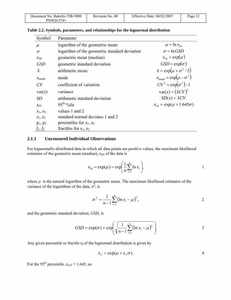
Table 2.2. Symbols, parameters, and relationships for the lognormal distribution
Symbol Parameter μ logarithm of the geometric mean 50ln x=μ σ logarithm of the geometric standard deviation GSDln=σ x50 geometric mean (median) ( )μexp50 =x GSD geometric standard deviation ( )σexp=GSD x arithmetic mean ( )2/exp 2σμ +=x xmode mode ( )2
mode exp σμ −=x CV coefficient of variation ( ) 1exp 22 −= σCV var(x) variance ( )2)var( CVxx = SD arithmetic standard deviation CVxxSD =)( x95 95th %ile )645.1exp(95 σμ +=x x1, x2 values 1 and 2 z1, z2 standard normal deviates 1 and 2 p1, p2 percentiles for x1, x2 f1, f2 fractiles for x1, x2
2.1.1 Uncensored Individual Observations
For lognormally-distributed data in which all data points are positive values, the maximum likelihood estimator of the geometric mean (median), x50, of the data is
,ln1exp)exp(1
50 ⎟⎠
⎞⎜⎝
⎛== ∑
=
n
iix
nx μ 1
where μ is the natural logarithm of the geometric mean. The maximum likelihood estimator of the variance of the logarithms of the data, σ2, is
( ) ,ln1
11
22 ∑=
−−
=n
iix
nμσ 2
and the geometric standard deviation, GSD, is
( ) .ln1
1exp)exp(1
2
⎟⎟⎠
⎞⎜⎜⎝
⎛−
−== ∑
=
n
iix
nGSD μσ 3
Any given percentile or fractile xf of the lognormal distribution is given by
).exp( σμ ff zx += 4
For the 95th percentile, z0.95 = 1.645, so

Document No. Battelle-TIB-5000 PNWD-3741
Revision No. 00 Effective Date: 04/02/2007 Page 13
).645.1exp(95 σμ +=x 5
2.1.2 Summary Statistics
There are many combinations of summary statistics from which a lognormal distribution can be uniquely defined. Strom and Stansbury (2000) described 15 methods, and a freeware program called LOGNORM4 can be downloaded1 to perform the calculations. The first 15 methods in Table 2.3 can be found using LOGNORM4, while method 16 is described in Section 2.1.2.3.
Table 2.3. Fifteen distinct ways of determining a lognormal distribution from minimal information
Method Determining Parameters 1 the mean and median (or their natural logs) 2 the mean and mode (or their natural logs) 3 the median and mode (or their natural logs) 4 the median (or its natural log) and the GSD or sigma = ln(GSD) 5 the mean (or its natural log) and the GSD or sigma = ln(GSD) 6 the mode (or its natural log) and the GSD or sigma = ln(GSD) 7 a value and its percentile OR fractile OR std norm deviate and GSD or sigma=ln(GSD) 8 the median and a value with its percentile OR fractile OR std normal deviate 9 the mean and a value with its percentile OR fractile OR std normal deviate
10 the mode and a value with its percentile OR fractile OR std normal deviate 11 the median and [arithmetic] standard deviation OR coefficient of variation 12 the mean and [arithmetic] standard deviation OR coefficient of variation 13 the mode and [arithmetic] standard deviation OR coefficient of variation 14 a value and its percentile OR fractile OR std norm deviate and [arithmetic] SD or CV 15 a pair of values and their percentiles OR fractiles OR std normal deviates 16 minimum, maximum, and mean values (see 2.1.2.3)
Sometimes data are reported in groups, e.g., airborne uranium concentration measurements from Eisenbud and Quigley (1956) shown in Table 2.4.
1 http://qecc.pnl.gov/LOGNORM4.htm
Document No. Battelle-TIB-5000 PNWD-3741
Revision No. 00 Effective Date: 04/02/2007 Page 14
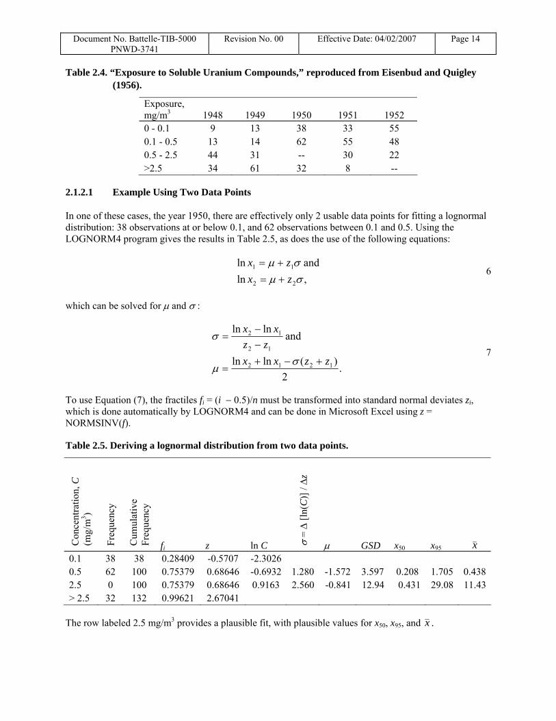
Table 2.4. “Exposure to Soluble Uranium Compounds,” reproduced from Eisenbud and Quigley (1956).
Exposure, mg/m3 1948 1949 1950 1951 1952 0 - 0.1 9 13 38 33 55 0.1 - 0.5 13 14 62 55 48 0.5 - 2.5 44 31 -- 30 22 >2.5 34 61 32 8 --
2.1.2.1 Example Using Two Data Points
In one of these cases, the year 1950, there are effectively only 2 usable data points for fitting a lognormal distribution: 38 observations at or below 0.1, and 62 observations between 0.1 and 0.5. Using the LOGNORM4 program gives the results in Table 2.5, as does the use of the following equations:
,lnand ln
22
11
σμσμ
zxzx
+=+=
6
which can be solved for μ and σ :
.
2)(lnln
and lnln
1212
12
12
zzxxzz
xx
+−+=
−−
=
σμ
σ 7
To use Equation (7), the fractiles fi = (i − 0.5)/n must be transformed into standard normal deviates zi, which is done automatically by LOGNORM4 and can be done in Microsoft Excel using z = NORMSINV(f).
Table 2.5. Deriving a lognormal distribution from two data points.
Con
cent
ratio
n, C
(m
g/m
3 )
Freq
uenc
y
Cum
ulat
ive
Freq
uenc
y
fi z ln C σ =
Δ [ln
(C)]
/ Δz
μ GSD x50 x95 x 0.1 38 38 0.28409 -0.5707 -2.3026 0.5 62 100 0.75379 0.68646 -0.6932 1.280 -1.572 3.597 0.208 1.705 0.438 2.5 0 100 0.75379 0.68646 0.9163 2.560 -0.841 12.94 0.431 29.08 11.43> 2.5 32 132 0.99621 2.67041
The row labeled 2.5 mg/m3 provides a plausible fit, with plausible values for x50, x95, and x .

Document No. Battelle-TIB-5000 PNWD-3741
Revision No. 00 Effective Date: 04/02/2007 Page 15
When only 2 data points are used to determine a lognormal distribution, there is no way to compute the uncertainty in the parameters.
2.1.2.2 Using Minimum, Mean, and Maximum Values with Number of Observations to Determine the Parameters of a Lognormal Distribution
When only minimum, mean, and maximum values are quoted but the number of observations is given, there are four possibilities.
• The minimum, maximum, and number of observations can be used with Equation (7) or LOGNORM4 to determine a lognormal distribution. However, in this case, one must examine the mean value predicted by the distribution and compare it to the observed mean. Note that this method even works with as few as two data points, which become the 25th and 75th percentiles of the resultant lognormal distribution.
• One can perform two additional fits using LOGNORM4 method 9 (Table 2.3), determining the lognormal parameters using the mean and a value with its percentile, fractile, or standard normal deviate. These two fits result in two more sets of lognormal distribution parameters. The analyst should examine these, and if they are reasonably similar, average them. If they are not reasonably similar, then the data were probably not lognormally distributed.
• Ignoring the number of observations, the minimum, maximum, and mean values can be used with the method in Section 2.1.2.3. The estimate of the number of data points produced by this method should be compared with the given number of observations for reasonableness.
If there is left-censoring, that is, if the minimum is quoted as “less than” some value, then only the second method will work and then only with the mean and maximum value.
2.1.2.3 Using Range and Mean Value without Number of Observations to Determine the Parameters of a Lognormal Distribution
When only a range and mean value are quoted, as in Christofano and Harris (1960), but the number of observations is not given, inference may become more difficult.
In principle, if the xmin and xmax values are symmetric about the geometric mean x50, then the 3 values uniquely determine a lognormal distribution. Under this assumption, fmin = 1 − fmax, so that −zmin = zmax, and it is easily shown that
.
or 2
lnln
maxmin50
maxmin
xxx
xx
=
+=μ
8
From the relationship ( )2/exp 2σμ +=x in Table 2.2, we find
.lnlnln2 maxmin2 xxx −−=σ 9
If the right hand side of equation 9 is negative or zero, a lognormal relationship is ruled out. If it is positive, then
Document No. Battelle-TIB-5000 PNWD-3741
Revision No. 00 Effective Date: 04/02/2007 Page 16
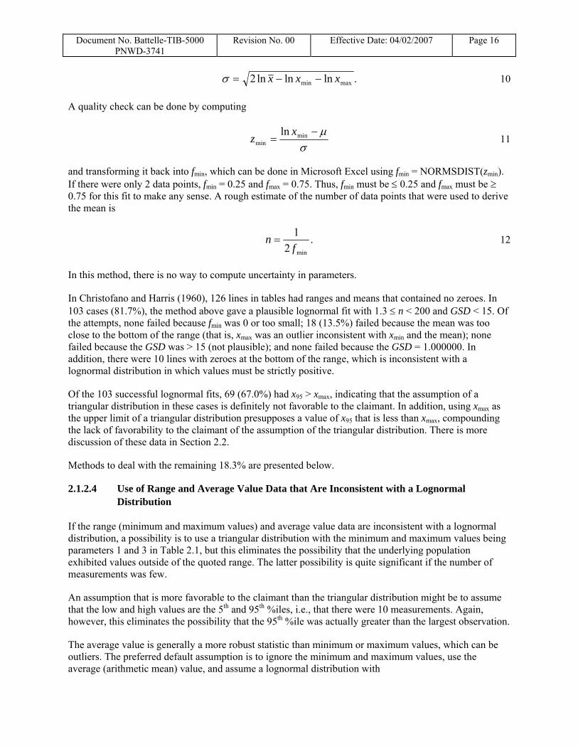
.lnlnln2 maxmin xxx −−=σ 10
A quality check can be done by computing
σ
μ−= min
minln x
z 11
and transforming it back into fmin, which can be done in Microsoft Excel using fmin = NORMSDIST(zmin). If there were only 2 data points, fmin = 0.25 and fmax = 0.75. Thus, fmin must be ≤ 0.25 and fmax must be ≥ 0.75 for this fit to make any sense. A rough estimate of the number of data points that were used to derive the mean is
.2
1
minfn = 12
In this method, there is no way to compute uncertainty in parameters.
In Christofano and Harris (1960), 126 lines in tables had ranges and means that contained no zeroes. In 103 cases (81.7%), the method above gave a plausible lognormal fit with 1.3 ≤ n < 200 and GSD < 15. Of the attempts, none failed because fmin was 0 or too small; 18 (13.5%) failed because the mean was too close to the bottom of the range (that is, xmax was an outlier inconsistent with xmin and the mean); none failed because the GSD was > 15 (not plausible); and none failed because the GSD = 1.000000. In addition, there were 10 lines with zeroes at the bottom of the range, which is inconsistent with a lognormal distribution in which values must be strictly positive.
Of the 103 successful lognormal fits, 69 (67.0%) had x95 > xmax, indicating that the assumption of a triangular distribution in these cases is definitely not favorable to the claimant. In addition, using xmax as the upper limit of a triangular distribution presupposes a value of x95 that is less than xmax, compounding the lack of favorability to the claimant of the assumption of the triangular distribution. There is more discussion of these data in Section 2.2.
Methods to deal with the remaining 18.3% are presented below.
2.1.2.4 Use of Range and Average Value Data that Are Inconsistent with a Lognormal Distribution
If the range (minimum and maximum values) and average value data are inconsistent with a lognormal distribution, a possibility is to use a triangular distribution with the minimum and maximum values being parameters 1 and 3 in Table 2.1, but this eliminates the possibility that the underlying population exhibited values outside of the quoted range. The latter possibility is quite significant if the number of measurements was few.
An assumption that is more favorable to the claimant than the triangular distribution might be to assume that the low and high values are the 5th and 95th %iles, i.e., that there were 10 measurements. Again, however, this eliminates the possibility that the 95th %ile was actually greater than the largest observation.
The average value is generally a more robust statistic than minimum or maximum values, which can be outliers. The preferred default assumption is to ignore the minimum and maximum values, use the average (arithmetic mean) value, and assume a lognormal distribution with

Document No. Battelle-TIB-5000 PNWD-3741
Revision No. 00 Effective Date: 04/02/2007 Page 17
• a GSD of 5 for data describing a single process (e.g., a series of air samples), or
• a GSD of 10 for data describing an entire site, plant, or factory.
The basis for assuming these GSDs derives from analyzing data from many facilities. The median (geometric mean) x50 is computed from the average (arithmetic mean) x using
),2/exp( 250 σ−= xx 13
where σ = ln(GSD).
Methods to deal with the remaining 18.3% are presented below.
2.1.2.5 Use of a Single Measurement Value
A single measurement is taken by metrologists to be the average or expectation value. Use the single result as the average (arithmetic mean) value, and assume a lognormal distribution with
• a GSD of 5 for data describing a single process (e.g., a series of air samples), or
• a GSD of 10 for data describing an entire site, plant, or factory.
The median (geometric mean) x50 is computed from the average (arithmetic mean) x using Eq. 13.
2.1.3 Censored Individual Observations
The simple method in 2.1.1 is not always available, especially in cases of left-censoring, grouping, and right-censoring.
2.1.3.1 Left-Censored Data
Sometimes values are reported as “less-than” some number or as zero. This is referred to as left-censoring. Since one cannot take the logarithm of zero or a less-than value, the method in 2.1.1 cannot be used. An alternative method consists of
• sorting the data in ascending order
• assigning fractiles fi = (i − 0.5)/n to each data point
• transforming the fractiles into standard normal deviates, zi
• taking the natural logarithm of the non-zero, non-censored values, ln xi
• using only the logs of non-zero, non-censored observations, perform a uniformly-weighted (i.e., unweighted) linear regression of ln xi as a function of zi
The slope of the linear regression is σ , and the intercept of the linear regression is μ . This method is described by Strom (1986) and probably many others.
Document No. Battelle-TIB-5000 PNWD-3741
Revision No. 00 Effective Date: 04/02/2007 Page 18
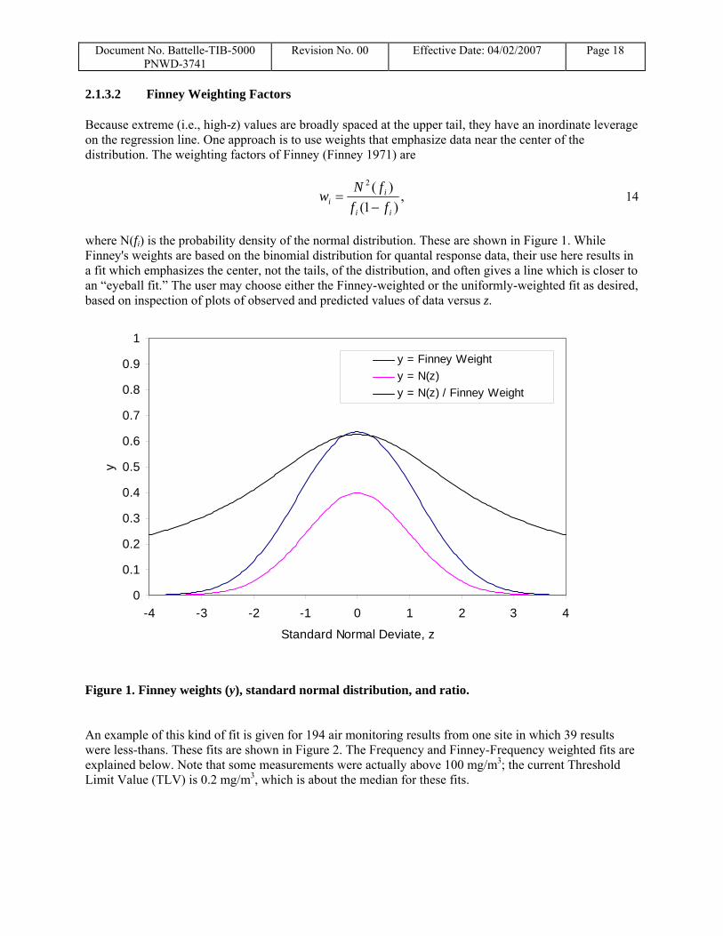
2.1.3.2 Finney Weighting Factors
Because extreme (i.e., high-z) values are broadly spaced at the upper tail, they have an inordinate leverage on the regression line. One approach is to use weights that emphasize data near the center of the distribution. The weighting factors of Finney (Finney 1971) are
,)1(
)(2
ii
ii ff
fNw−
= 14
where N(fi) is the probability density of the normal distribution. These are shown in Figure 1. While Finney's weights are based on the binomial distribution for quantal response data, their use here results in a fit which emphasizes the center, not the tails, of the distribution, and often gives a line which is closer to an “eyeball fit.” The user may choose either the Finney-weighted or the uniformly-weighted fit as desired, based on inspection of plots of observed and predicted values of data versus z.
0
0.1
0.2
0.3
0.4
0.5
0.6
0.7
0.8
0.9
1
-4 -3 -2 -1 0 1 2 3 4
Standard Normal Deviate, z
y
y = Finney Weighty = N(z)y = N(z) / Finney Weight
Figure 1. Finney weights (y), standard normal distribution, and ratio.
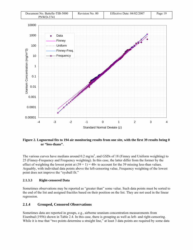
An example of this kind of fit is given for 194 air monitoring results from one site in which 39 results were less-thans. These fits are shown in Figure 2. The Frequency and Finney-Frequency weighted fits are explained below. Note that some measurements were actually above 100 mg/m3; the current Threshold Limit Value (TLV) is 0.2 mg/m3, which is about the median for these fits.
Document No. Battelle-TIB-5000 PNWD-3741
Revision No. 00 Effective Date: 04/02/2007 Page 19
0.00001
0.0001
0.001
0.01
0.1
1
10
100
1000
10000
-4 -3 -2 -1 0 1 2 3 4
Standard Normal Deviate (z)
Ura
nium
Con
cent
ratio
n (m
g/m
^3)
DataFinneyUniformFinney-Freq.Frequency
Figure 2. Lognormal fits to 194 air monitoring results from one site, with the first 39 results being 0 or “less-thans”.
The various curves have medians around 0.2 mg/m3, and GSDs of 18 (Finney and Uniform weighting) to 25 (Finney-Frequency and Frequency weighting). In this case, the latter differ from the former by the effect of weighting the lowest point at (39 + 1) = 40× to account for the 39 missing less-than values. Arguably, with individual data points above the left-censoring value, Frequency weighting of the lowest point does not improve the “eyeball fit.”
2.1.3.3 Right-censored Data
Sometimes observations may be reported as “greater than” some value. Such data points must be sorted to the end of the list and assigned fractiles based on their position on the list. They are not used in the linear regression.
2.1.4 Grouped, Censored Observations
Sometimes data are reported in groups, e.g., airborne uranium concentration measurements from Eisenbud (1956) shown in Table 2.4. In this case, there is grouping as well as left- and right-censoring. While it is true that “two points determine a straight line,” at least 3 data points are required by some data

Document No. Battelle-TIB-5000 PNWD-3741
Revision No. 00 Effective Date: 04/02/2007 Page 20
fitting routines that calculate statistics other than the slope and the intercept. This method is described by Strom (1986) and probably many others.
2.1.4.1 Frequency Weighting for Grouped Data
Grouped, censored observations will require additional weighting considerations. The first data point in 1949 represents 13 of the 119 total observations; the second, 14; the third, 31, and the final point, 64. The fit will generally be improved if each point is weighed by the number of observations it represents. In addition, a weighting factor that accounts for both frequency and weights data near the median can be created by multiplying the frequency by the Finney weight described in Section 2.1.3.2.
An example of fitting a lognormal distribution to grouped, left- and right-censored data is shown in Figure 3, the 1949 data from Table 2.4. With more than half of the observations greater than the median, the upper 95th %ile is very large.
0.001
0.01
0.1
1
10
100
1000
10000
-3 -2 -1 0 1 2 3Standard Normal Deviate (z)
Ura
nium
Con
cent
ratio
n (m
g/m
^3)
DataFinneyUniformFinney-Freq.Frequency
Figure 3. Examples of fitting a lognormal distribution to grouped, left- and right-censored data (from Table 7, 1949, Eisenbud and Quigley 1956)
Document No. Battelle-TIB-5000 PNWD-3741
Revision No. 00 Effective Date: 04/02/2007 Page 21
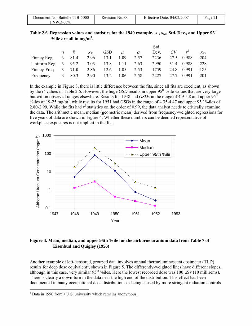
Table 2.6. Regression values and statistics for the 1949 example. x , x50, Std. Dev., and Upper 95th %ile are all in mg/m3.
n x x50 GSD μ σ Std. Dev. CV r2 x95
Finney Reg 3 81.4 2.96 13.1 1.09 2.57 2236 27.5 0.988 204 Uniform Reg 3 95.2 3.03 13.8 1.11 2.63 2990 31.4 0.988 228 Finney-Freq 3 71.0 2.86 12.6 1.05 2.53 1759 24.8 0.991 185 Frequency 3 80.3 2.90 13.2 1.06 2.58 2227 27.7 0.991 201
In the example in Figure 3, there is little difference between the fits, since all fits are excellent, as shown by the r2 values in Table 2.6. However, the huge GSD results in upper 95th %ile values that are very large but within observed ranges elsewhere. Results for 1948 had GSDs in the range of 4.9-5.8 and upper 95th %iles of 19-25 mg/m3, while results for 1951 had GSDs in the range of 4.35-4.47 and upper 95th %iles of 2.80-2.99. While the fits had r2 statistics on the order of 0.99, the data analyst needs to critically examine the data. The arithmetic mean, median (geometric mean) derived from frequency-weighted regressions for five years of data are shown in Figure 4. Whether these numbers can be deemed representative of workplace exposures is not implicit in the fits.
0.1
1
10
100
1000
1947 1948 1949 1950 1951 1952 1953
Year
Airb
orne
Ura
nium
Con
cent
ratio
n (m
g/m
3 )
MeanMedianUpper 95th %ile
Figure 4. Mean, median, and upper 95th %ile for the airborne uranium data from Table 7 of Eisenbud and Quigley (1956)
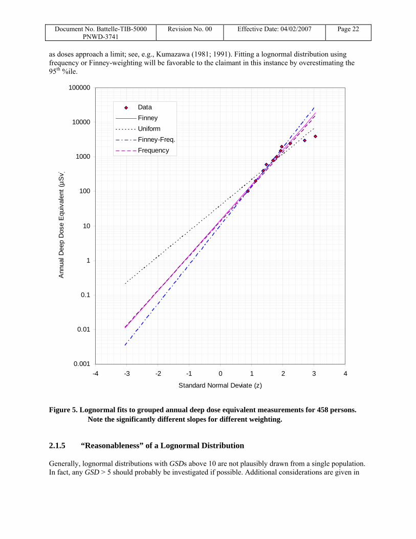
Another example of left-censored, grouped data involves annual thermoluminescent dosimeter (TLD) results for deep dose equivalent2, shown in Figure 5. The differently-weighted lines have different slopes, although in this case, very similar 95th %iles. Here the lowest recorded dose was 100 µSv (10 millirems). There is clearly a down-turn in the data near the high end of the distribution. This effect has been documented in many occupational dose distributions as being caused by more stringent radiation controls 2 Data in 1990 from a U.S. university which remains anonymous.
Document No. Battelle-TIB-5000 PNWD-3741
Revision No. 00 Effective Date: 04/02/2007 Page 22
as doses approach a limit; see, e.g., Kumazawa (1981; 1991). Fitting a lognormal distribution using frequency or Finney-weighting will be favorable to the claimant in this instance by overestimating the 95th %ile.
0.001
0.01
0.1
1
10
100
1000
10000
100000
-4 -3 -2 -1 0 1 2 3 4
Standard Normal Deviate (z)
Ann
ual D
eep
Dos
e E
quiv
alen
t (µS
v)
DataFinneyUniformFinney-Freq.Frequency
Figure 5. Lognormal fits to grouped annual deep dose equivalent measurements for 458 persons. Note the significantly different slopes for different weighting.
2.1.5 “Reasonableness” of a Lognormal Distribution
Generally, lognormal distributions with GSDs above 10 are not plausibly drawn from a single population. In fact, any GSD > 5 should probably be investigated if possible. Additional considerations are given in
Document No. Battelle-TIB-5000 PNWD-3741
Revision No. 00 Effective Date: 04/02/2007 Page 23
Section 3.7 and 3.8. A lognormal may still be a better choice than other distributions accommodated by IREP.
2.1.6 Summary of Default Assumptions for Fitting Lognormal Distributions
In summary, different methods of determining the geometric mean, geometric standard deviation, and upper 95th %ile are needed for 4 different kinds of data.
If there is no censoring, estimate μ and σ from the average and standard deviation of the natural logarithms of the data, and compute any needed statistics from there as shown in Section 2.1.1. It still may be wise to perform weighted linear regressions and examine plots of the data with the predictions.
If only summary statistics are available, such as the mean and standard deviation of observations, use the methods in Strom and Stansbury (2000), which are implemented in freeware LOGNORM4, or the equations in Section 2.1.2. It is sometimes possible to generate a lognormal from a range and a mean value, but the analyst must still look at the reasonableness of the resulting distribution. Fitting a lognormal to a minimum-mean-maximum data triad will almost always produce a higher 95%ile value than fitting a triangular distribution.
If individual observations are available, but there is left-censoring, right censoring, or both, perform weighted linear regressions of the uncensored observations xi against their known standard normal deviates zi, and examine various weighting schemes, e.g., uniform-, Finney-, and frequency-weighting, as described in Section 2.1.3.
If only grouped data are available, which are inherently left-censored and may or may not be right-censored, perform a frequency-weighted linear regression of the uncensored group upper limits xi against the known standard normal deviates zi, using the methods described in Section 2.1.4. The analyst is encouraged to examine various other weighting schemes, e.g., uniform-, Finney-, and frequency-weighting.
In each of the four cases, the data analyst should qualitatively determine whether the fitted lognormal distribution makes reasonable predictions.
2.2 Triangular Distributions
There is little information available on the use of triangular distributions from NIOSH/OCAS, although they are available in IREP. Like the uniform distribution, the triangular distribution has absolute limits below or above which the distribution is zero (Brighton Webs Ltd. 2006; Weisstein 2006; Wikipedia 2006). Such is not the case for the normal and lognormal distributions, although they have effective upper and lower bounds.
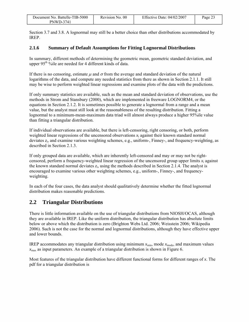
IREP accommodates any triangular distribution using minimum xmin, mode xmode, and maximum values xmax as input parameters. An example of a triangular distribution is shown in Figure 6.
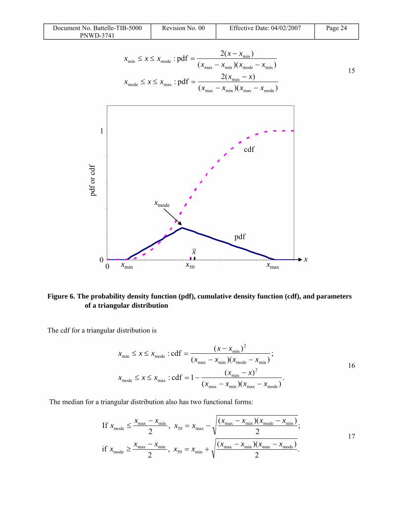
Most features of the triangular distribution have different functional forms for different ranges of x. The pdf for a triangular distribution is
Document No. Battelle-TIB-5000 PNWD-3741
Revision No. 00 Effective Date: 04/02/2007 Page 24
))(()(2pdf:
))(()(2pdf:
modemaxminmax
maxmaxmode
minmodeminmax
minmodemin
xxxxxxxxx
xxxxxxxxx
−−−
=≤≤
−−−
=≤≤
15
x
pdf o
r cdf
x50
x
xmode
xmin xmax
1
00
cdf
Figure 6. The probability density function (pdf), cumulative density function (cdf), and parameters of a triangular distribution
The cdf for a triangular distribution is
.))((
)(1cdf:
;))((
)(cdf:
modemaxminmax
2max
maxmode
minmodeminmax
2min
modemin
xxxxxxxxx
xxxxxxxxx
−−−
−=≤≤
−−−
=≤≤
16
The median for a triangular distribution also has two functional forms:
.2
))(( ,2
if
;2
))(( ,2
If
modemaxminmaxmin50
minmaxmode
minmodeminmaxmax50
minmaxmode
xxxxxxxxx
xxxxxxxxx
−−+=
−≥
−−−=
−≤
17
Document No. Battelle-TIB-5000 PNWD-3741
Revision No. 00 Effective Date: 04/02/2007 Page 25
The derivation of the three general parameters of the triangular distribution from data values such as mean and range is straightforward. Since the mean of a triangular distribution is
,3
modemaxmin xxxx ++= 18
the mode can be obtained by
.3 maxminmode xxxx −−= 19
The inequality
maxmodemin xxx ≤≤ 20
must hold or a triangular distribution is inconsistent with the data.
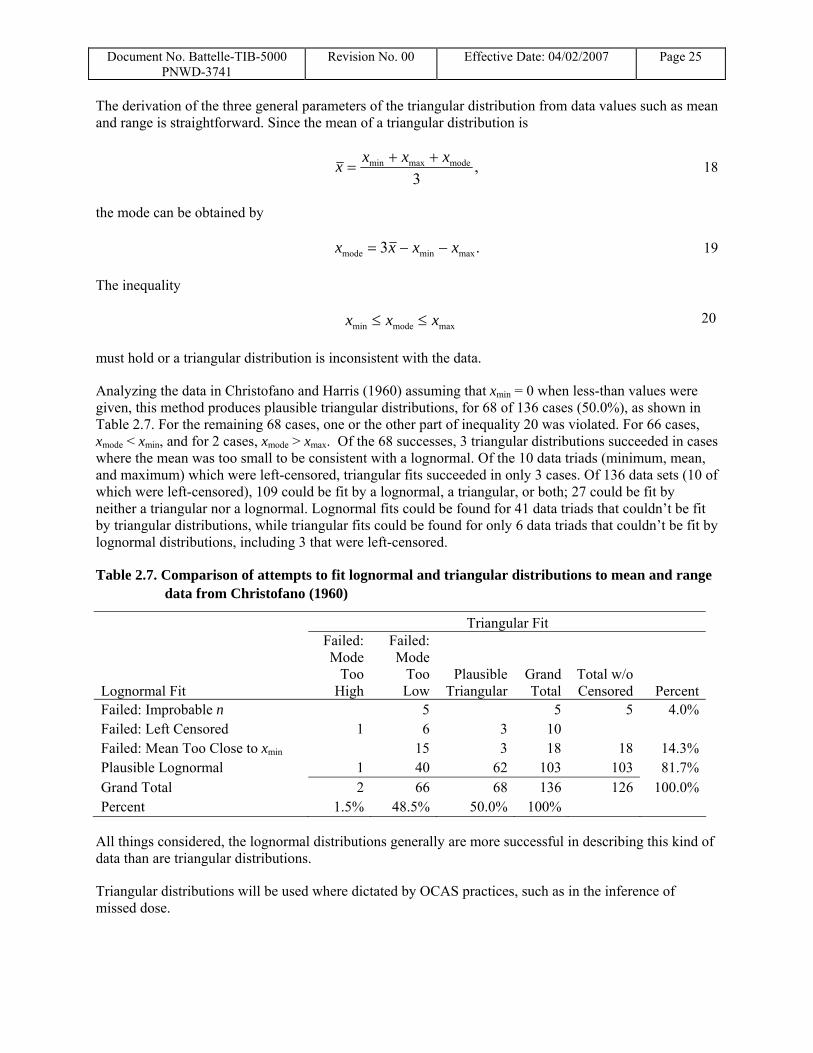
Analyzing the data in Christofano and Harris (1960) assuming that xmin = 0 when less-than values were given, this method produces plausible triangular distributions, for 68 of 136 cases (50.0%), as shown in Table 2.7. For the remaining 68 cases, one or the other part of inequality 20 was violated. For 66 cases, xmode < xmin, and for 2 cases, xmode > xmax. Of the 68 successes, 3 triangular distributions succeeded in cases where the mean was too small to be consistent with a lognormal. Of the 10 data triads (minimum, mean, and maximum) which were left-censored, triangular fits succeeded in only 3 cases. Of 136 data sets (10 of which were left-censored), 109 could be fit by a lognormal, a triangular, or both; 27 could be fit by neither a triangular nor a lognormal. Lognormal fits could be found for 41 data triads that couldn’t be fit by triangular distributions, while triangular fits could be found for only 6 data triads that couldn’t be fit by lognormal distributions, including 3 that were left-censored.
Table 2.7. Comparison of attempts to fit lognormal and triangular distributions to mean and range data from Christofano (1960)
Triangular Fit
Lognormal Fit
Failed: Mode
Too High
Failed: Mode
Too Low
Plausible Triangular
Grand Total
Total w/o Censored Percent
Failed: Improbable n 5 5 5 4.0%Failed: Left Censored 1 6 3 10 Failed: Mean Too Close to xmin 15 3 18 18 14.3%Plausible Lognormal 1 40 62 103 103 81.7%Grand Total 2 66 68 136 126 100.0%Percent 1.5% 48.5% 50.0% 100%
All things considered, the lognormal distributions generally are more successful in describing this kind of data than are triangular distributions.
Triangular distributions will be used where dictated by OCAS practices, such as in the inference of missed dose.
Document No. Battelle-TIB-5000 PNWD-3741
Revision No. 00 Effective Date: 04/02/2007 Page 26
2.3 Normal Distributions
Because of Ott’s argument, stated in Section 2.1, it is unlikely that most exposure parameters have normally-distributed uncertainties. Exceptions are bioassay and dose measurements associated with individuals. In these cases, often information is available concerning the mean value, and sometimes the standard deviation. The uncertainty of standard measurements such as film dosimetry can often be inferred from the literature.
2.3.1 Normally-distributed Measurement Uncertainty and an Underlying Lognormally-distributed Measurand: Mirror Image Method
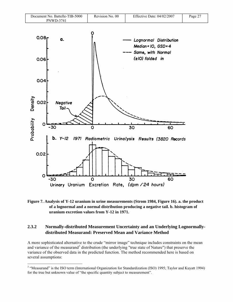
In cases where the standard deviation is unknown, and negative values have been observed and recorded, it is possible to analyze the negative tails using the “mirror image” procedure suggested by Strom (1984; 1984). In that method, the negative tail of the observed distribution is reflected about the ordinate, and the standard deviation of the resulting distribution is used to estimate the measurement uncertainty. A preliminary version of the method was used in 1983 to deduce measurements uncertainty in uranium urinalysis results at the Y-12 plant in Oak Ridge, Tennessee (Strom 1984). An example for 1971 results is shown in Figure 7.
Document No. Battelle-TIB-5000 PNWD-3741
Revision No. 00 Effective Date: 04/02/2007 Page 27
Figure 7. Analysis of Y-12 uranium in urine measurements (Strom 1984, Figure 16). a. the product of a lognormal and a normal distribution producing a negative tail. b. histogram of uranium excretion values from Y-12 in 1971.
2.3.2 Normally-distributed Measurement Uncertainty and an Underlying Lognormally-distributed Measurand: Preserved Mean and Variance Method
A more sophisticated alternative to the crude “mirror image” technique includes constraints on the mean and variance of the measurand3 distribution (the underlying "true state of Nature") that preserve the variance of the observed data in the predicted function. The method recommended here is based on several assumptions: 3 “Measurand” is the ISO term (International Organization for Standardization (ISO) 1995; Taylor and Kuyatt 1994) for the true but unknown value of “the specific quantity subject to measurement”.
Document No. Battelle-TIB-5000 PNWD-3741
Revision No. 00 Effective Date: 04/02/2007 Page 28
1. The observed probability density function (pdf) is the result of combining a normally-distributed measurement uncertainty with a lognormally-distributed measurand.
2. The mean of the lognormal “true state of nature” is equal to the mean of the observations.
3. Measurements are unbiased, so the mean of the measurement uncertainty distribution is zero.
4. The variance of the observed values is equal to the sum of the variance of the measurement uncertainty plus the variance of the lognormal “true state of nature.”
Since the uncertainty distribution is characterized by a mean and standard deviation (or variance), and the lognormal “true state of nature” is characterized by a median and a geometric standard deviation (GSD), there are only 4 adjustable parameters. The assumptions listed above constrain the problem so that only one parameter can be freely adjusted, either the standard deviation of the uncertainty distribution or the GSD of the lognormal. For this analysis, it is recommended that the GSD of the lognormal be chosen as the varying parameter.
The best fit for this purpose cannot be arrived at by a single “goodness of fit” statistical test, such as Kolmogov-Smirnoff, Cramer-Von Mises, or a runs test. Examining of the residuals for the fits reveals systematic but not large differences in the observations from the assumptions above.
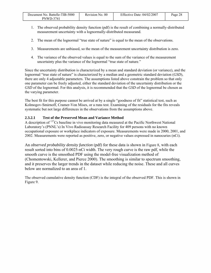
2.3.2.1 Test of the Preserved Mean and Variance Method A description of 137Cs baseline in vivo monitoring data measured at the Pacific Northwest National Laboratory’s (PNNL’s) In Vivo Radioassay Research Facility for 409 persons with no known occupational exposure or workplace indicators of exposure. Measurements were made in 2000, 2001, and 2002. Measurements were reported as positive, zero, or negative values expressed in nanocuries (nCi). An observed probability density function (pdf) for these data is shown in Figure 8, with each result sorted into bins of 0.0025-nCi width. The very rough curve is the raw pdf, while the smooth curve is the smoothed PDF using the model-free visualization method of (Chomentowski, Kellerer, and Pierce 2000). The smoothing is similar to spectrum smoothing, and it preserves the larger trends in the dataset while reducing the noise. These and all curves below are normalized to an area of 1. The observed cumulative density function (CDF) is the integral of the observed PDF. This is shown in Figure 9.
Document No. Battelle-TIB-5000 PNWD-3741
Revision No. 00 Effective Date: 04/02/2007 Page 29
0
1
2
3
4
5
6
7
-1 -0.5 0 0.5 1 1.5 2137Cs (nCi)
His
togr
am o
r Sm
ooth
ed p
df (n
Ci-1
)pdfSmoothed pdf
Figure 8. Normalized probability density functions (pdfs) for Hanford in vivo 137Cs measurements on unexposed workers
0
0.1
0.2
0.3
0.4
0.5
0.6
0.7
0.8
0.9
1
-0.6 -0.4 -0.2 0 0.2 0.4 0.6 0.8 1137Cs (nCi)
cdf
Predicted cdfObserved cdf
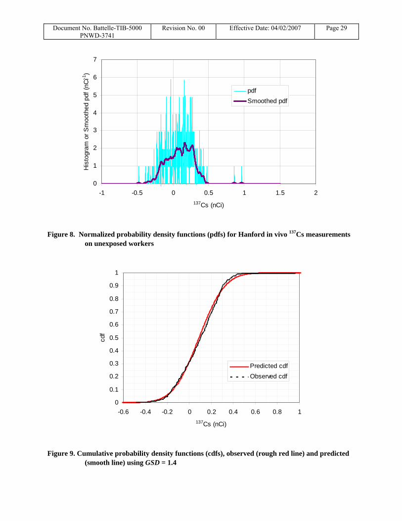
Figure 9. Cumulative probability density functions (cdfs), observed (rough red line) and predicted (smooth line) using GSD = 1.4
Document No. Battelle-TIB-5000 PNWD-3741
Revision No. 00 Effective Date: 04/02/2007 Page 30
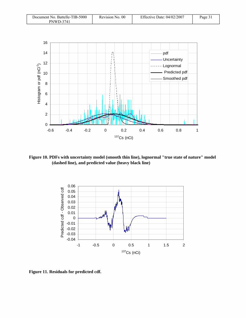
The best fits were lognormals with mean = 0.0936 nCi (the mean of the data), GSDs of 1.2, 1.4, or 1.6 (medians of 0.0921, 0.0885, and 0.0838 nCi, respectively), and uncertainty distributions with standard deviations of 0.180 to 0.185 nCi. The results for GSD = 1.4 are shown in Figure 10 and Figure 11. These three were essentially indistinguishable, given the observed 137Cs values. The model developed here assumes that observations arise from a lognormal “true state of nature” (dashed curve in Figure 10) filtered through the lens of a normal measurement uncertainty. This model provides an adequate fit to the data, although the choice of GSD (and related parameters) is not obvious but lies in the range of 1.2 to 1.6. Figure 11 shows the residuals for the predicted cdf shown in Figure 9. Examining of the residuals for the fits reveals systematic but not large differences in the observed 137Cs population from the assumptions above. The mean uncertainty of the observations was 0.191 nCi, slightly larger than any uncertainty consistent with the assumptions above. Clearly there are clusters of points here and there in the observed distribution, but overall, the predicted cdf in Figure 9 is close to the observed cdf.
Document No. Battelle-TIB-5000 PNWD-3741
Revision No. 00 Effective Date: 04/02/2007 Page 31
0
2
4
6
8
10
12
14
16
-0.6 -0.4 -0.2 0 0.2 0.4 0.6 0.8 1137Cs (nCi)
His
togr
am o
r pdf
(nC
i-1)
pdfUncertaintyLognormal Predicted pdfSmoothed pdf
Figure 10. PDFs with uncertainty model (smooth thin line), lognormal "true state of nature" model (dashed line), and predicted value (heavy black line)
-0.04-0.03-0.02-0.01
00.010.020.030.040.050.06
-1 -0.5 0 0.5 1 1.5 2137Cs (nCi)
Pre
dict
ed c
df -
Obs
erve
d cd
f
Figure 11. Residuals for predicted cdf.

Document No. Battelle-TIB-5000 PNWD-3741
Revision No. 00 Effective Date: 04/02/2007 Page 32
If a non-occupationally exposed population has retained quantities of 137Cs that are lognormally distributed with means of 0.0936 and GSDs of 1.2, 1.4, or 1.6 as shown in the table, then the specified percent of them will have retained quantities equal to or exceeding the Table 2.8 values in nCi.
Table 2.8. 90, 95, and 99 %iles of lognormal "true state of nature" distributions with GSDs of 1.2, 1.4, and 1.6.
%ile %
exceeding 1.2 1.4 1.6 90 10 0.116 0.136 0.15395 5 0.124 0.154 0.18299 1 0.141 0.194 0.250
It is clear that the 95 %ile values are on the order of the standard deviation of the measurements, typically 0.19 nCi. In measuring 409 persons at Hanford with no reason to expect an occupational intake, one observes that the results are at or above 0.35 nCi 5% of the time. The fact that this value is nearly double the largest value in Table 2.8, and about twice the average measurement uncertainty of 0.19 nCi is due to the fact that the measurement uncertainty is just over twice as large as the average measured value.
In the absence of workplace indicators, one concludes that a 137Cs measurement result of 0.35 nCi has a more than 5% chance of being due to environmental exposure and measurement uncertainty.
The method illustrated here can be used to determine the likelihood of an individual exceeding a particular exposure or dose level when uncensored data are available.
2.4 Rectangular Distributions
IREP can accept a rectangular distribution as input. A rectangular distribution consists of 2 values, and upper and a lower bound that are believed to bracket the range of plausible values of concentration, intake, dose, or dose rate. Rectangular distributions are non-physical, but can be used to represent a limited state of knowledge.
2.5 Constant “Distributions”
IREP can accept a constant distribution as input. A constant distribution is a single number, generally taken as an overestimate that is favorable to the claimant of a concentration, intake, dose, or dose rate. See section 3.3.

Document No. Battelle-TIB-5000 PNWD-3741
Revision No. 00 Effective Date: 04/02/2007 Page 33
3.0 Default Assumptions
3.1 Introduction
There are science policy and expert judgment issues that must be considered in dose reconstruction.
This section contains assumptions about • external irradiation geometry • use of the 95th %ile for air sample distributions • uncertainty in biokinetic models • aerosol particle size and respirable fraction • use of time-period-specific, process-based GSDs for published mean aerosol concentration data • use of time-weighted averages, breathing-zone (BZ) air samples, and general area (GA) air
samples, and considerations of sample duration • particle solubility (ICRP 66 transportability classes F, M, S) and f1 (gastrointestinal absorption
fractions) • exposure time • ingestion • occupational medical doses • external dose conversion factors • external missed dose when there was monitoring • internal missed dose when there was monitoring • environmental dose • radon and thoron and their short-lived decay products
3.2 External Irradiation Geometry
Default assumptions of irradiation geometry may be reasonably justified, as described in Table 4.2 on page 53 of NIOSH OCAS-IG-001 (2002). The “job” entries in that table for uranium facilities have been generalized for all of the job categories found among claimants in the cases covered by this TIB. These are detailed in a 326-line spreadsheet entitled “Irradiation_Geometry_by_Job_Title.xls”. To make these choices, and experienced IH assigned job titles to
• the “general (roamer)” category denoted in IG-001 as “General Laborer”
• the “operator (doer)” category denoted in IG-001 as “Machinist”
• the “white collar (supervisor)” category denoted in IG-001 as “Supervisor” or
• the “not assigned” category (44 job titles) that have to be elaborated from additional information or, failing that, will be assigned the maximum DCF values.

Document No. Battelle-TIB-5000 PNWD-3741
Revision No. 00 Effective Date: 04/02/2007 Page 34
3.3 The 95%ile and “Constant” Uncertainty Distribution for Limited Data Sets
Sometimes one must infer exposures from a small set of measurements such as a few air samples taken at various locations at a facility. The inference is that the distribution these samples represent applies to the entire facility. For people who move around, such as crafts and maintenance personnel, the average may be appropriate. However, if it is credible that a claimant routinely worked in one of the higher airborne areas, this distribution does not fairly represent the individual’s exposure. To account for this, one infers that the individual was exposed to the 95th percentile of the distribution. Another example is a distribution of a few film badges. If these are the result of only a few representative monitored workers, it is credible that any particular claimant could really represent the upper end of that distribution. According to a communication from NIOSH, use of the 95th %ile assumption has expanded recently and is used in more and more situations. In any case, the 95th percentile is considered to represent the upper bound of the exposure. Any exposures calculated from this are entered into IREP as a constant.
3.4 Uncertainty in Biokinetic Models
The National Council on Radiation Protection and Measurements (NCRP) used an expert group of internal dosimetrists to create a subjective quantification of the reliability of ICRP Publication 30 biokinetic and dosimetric models (National Council on Radiation Protection and Measurements (NCRP) 1998). While IMBA uses the newer ICRP Publication 66 respiratory tract model and newer biokinetic models, the results of these models may not be that much better than the ICRP 30 models for some radionuclides in cases where f1 is the dominant uncertainty. NCRP developed “Reliability Categories” A through D, as described in Table 3.1. The two right hand columns were developed in this work for lognormal distributions consistent with the NCRP criteria.
Table 3.1. Reliability categories for selected results of ICRP Publication 30 biokinetic and dosimetric models
Reliability categories For at least 90% of a Group, does the
effective dose coefficient E(i) lie 5095 / xx GSD if
lognormal "well known" A Between E(i)/3 and E(i)*3 3 ≤1.95 "reasonably well known"
B outside the previous range, but between E(i)/5 and E(i)*5
5 1.95≤ GSD ≤ 2.66
"poorly known" C outside the previous range, but between E(i)/10 and E(i)*10
10 2.66 ≤ GSD ≤ 4.05
"very poorly known" D outside the previous range >10 GSD > 4.05
The NCRP experts ranked each of 26 radionuclides for a) healthy adult males, and b) special populations of infants, diseased people, (and presumably women, who are not “healthy adult males”). Some radionuclides were also ranked separately for ingestion intakes and inhalation intakes. Rankings for thorium and uranium are given in Table 3.2.
Document No. Battelle-TIB-5000 PNWD-3741
Revision No. 00 Effective Date: 04/02/2007 Page 35
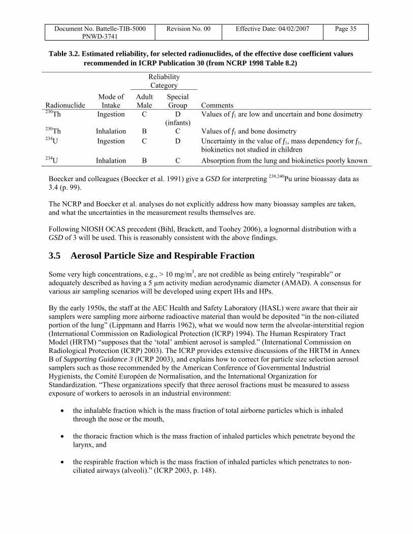
Table 3.2. Estimated reliability, for selected radionuclides, of the effective dose coefficient values recommended in ICRP Publication 30 (from NCRP 1998 Table 8.2)
Reliability Category
Radionuclide Mode of Intake
Adult Male
Special Group Comments
230Th Ingestion C D (infants)
Values of f1 are low and uncertain and bone dosimetry
230Th Inhalation B C Values of f1 and bone dosimetry 234U Ingestion C D Uncertainty in the value of f1, mass dependency for f1,
biokinetics not studied in children 234U Inhalation B C Absorption from the lung and biokinetics poorly known
Boecker and colleagues (Boecker et al. 1991) give a GSD for interpreting 239,240Pu urine bioassay data as 3.4 (p. 99).
The NCRP and Boecker et al. analyses do not explicitly address how many bioassay samples are taken, and what the uncertainties in the measurement results themselves are.
Following NIOSH OCAS precedent (Bihl, Brackett, and Toohey 2006), a lognormal distribution with a GSD of 3 will be used. This is reasonably consistent with the above findings.
3.5 Aerosol Particle Size and Respirable Fraction
Some very high concentrations, e.g., > 10 mg/m3, are not credible as being entirely “respirable” or adequately described as having a 5 µm activity median aerodynamic diameter (AMAD). A consensus for various air sampling scenarios will be developed using expert IHs and HPs.
By the early 1950s, the staff at the AEC Health and Safety Laboratory (HASL) were aware that their air samplers were sampling more airborne radioactive material than would be deposited “in the non-ciliated portion of the lung” (Lippmann and Harris 1962), what we would now term the alveolar-interstitial region (International Commission on Radiological Protection (ICRP) 1994). The Human Respiratory Tract Model (HRTM) “supposes that the ‘total’ ambient aerosol is sampled.” (International Commission on Radiological Protection (ICRP) 2003). The ICRP provides extensive discussions of the HRTM in Annex B of Supporting Guidance 3 (ICRP 2003), and explains how to correct for particle size selection aerosol samplers such as those recommended by the American Conference of Governmental Industrial Hygienists, the Comité Européen de Normalisation, and the International Organization for Standardization. “These organizations specify that three aerosol fractions must be measured to assess exposure of workers to aerosols in an industrial environment:
• the inhalable fraction which is the mass fraction of total airborne particles which is inhaled through the nose or the mouth,
• the thoracic fraction which is the mass fraction of inhaled particles which penetrate beyond the larynx, and
• the respirable fraction which is the mass fraction of inhaled particles which penetrates to non-ciliated airways (alveoli).” (ICRP 2003, p. 148).
Document No. Battelle-TIB-5000 PNWD-3741
Revision No. 00 Effective Date: 04/02/2007 Page 36
The HRTM is only correct if the true AMAD of the aerosol is used and if the entire aerosol is sampled. If an aerosol has a true AMAD of 30, 20 or 10 µm but is modeled as having an AMAD of 5 µm, the resultant dose estimates for uranium will be high by factors of x, y, and z, respectively.
Default assumptions of ICRP Pub. 66, i.e., 5 µm AMAD, will be used in the absence of other information.
3.6 Use of Time-period-specific, Process-based GSDs for Published Mean Aerosol Concentration Data
Pending review and additional justification, the current default assumption when no information is available on uncertainty in aerosol measurements is that they are lognormally-distributed with a GSD of 5 for a single process or activity, and 10 for an entire site, plant, or factory. These choices are based on an analysis of data from Christofano and Harris (1960).
In that paper, as mentioned in Section 2.1.2.4, there were 108 instances when a lognormal distribution could be fit to tabulated data. The GSDs of those lognormal distributions ranged from 1.13 to 12.8, with an average of 2.89 + 1.58 (at 1 standard deviation), a geometric mean of 2.59 ×÷ 1.56, and an upper 95th percentile of ~5.2. Based on this analysis, for single processes, it is reasonably favorable to the claimant to choose a GSD of 5 as a default when there is no other way to estimate the GSD.
Looking at all 136 process-specific mean airborne U concentrations reported in Christofano and Harris (1960), one arrives as the analysis shown in Figure 12. These values are roughly lognormally distributed, with GSDs ranging from 9.0 to 10.4, depending on the weighting method chosen. Based on this analysis, for site-wide data, it is reasonably favorable to the claimant to choose a GSD of 10 as a default when there is no other way to estimate the GSD.

Document No. Battelle-TIB-5000 PNWD-3741
Revision No. 00 Effective Date: 04/02/2007 Page 37
0.1
1
10
100
1000
10000
100000
1000000
-3 -2 -1 0 1 2 3Standard Normal Deviate, z
Airb
orne
U C
once
ntra
tion
(dpm
/m3 )
Sorted Dataln(Data) Pred. GM= 523. GSD= 9.16Uniform Pred. GM= 523. GSD= 9.01Finney Pred. GM= 475. GSD= 10.4
Figure 12. Lognormal plot of mean airborne U concentrations for 136 different processes in uranium refining (Christofano and Harris 1960).
Currently, when a single value is available, it is assumed to be the mean ( x ; also known as the expectation value, the arithmetic mean, and the average) of the resultant lognormal distribution. The median (x50; also known as the geometric mean), which is always less than the mean for lognormally-distributed data, is calculated from the mean and the GSD using Eq. 31. The median and the GSD are the parameters required by IREP for any lognormally-distributed quantity.
3.7 Use of Distributions to Describe Multiple Populations
Statistical distributions such as the lognormal are used to describe observations of single populations, e.g., the distribution of body mass of adult people. One does not generally use distributions to model combined populations, e.g., body masses of infants and body masses of adults, or body masses of microbes, insects and mammals. However, it may be necessary to combine all air samples for a single plant to describe the exposures of workers who are “roamers” (Section 3.2) or for whom no description of job duties or locations is available.
It is possible to combine breathing zone (BZ) air sample results for different processes and describe the combined data with a statistical distribution, but it is difficult to imagine what such a distribution signifies
Document No. Battelle-TIB-5000 PNWD-3741
Revision No. 00 Effective Date: 04/02/2007 Page 38
unless one has a specific end in mind. One could, for example combine BZ results for “furnace operators” and “fork lift operators” and use the result to describe exposures to “operators” of an unspecified type.
It is possible to combine air samples that were taken for a fraction of a minute during the “dirtiest” part of batch processes, e.g., dumping ore from a drum into a process bin or chipping out a crucible, with air samples that were taken over a period of hours during continuous processes. Again, it is difficult to know what such a distribution of combined results would represent. The short-duration air samples were probably taken as worst-case values, while the longer-term samples may have represented average values to which workers may have had prolonged exposures.
One data set, shown in Figure 2, is not, in the judgment of a panel of health physicists and industrial hygienists, taken from the same population. They may be a combination of incommensurate values.
It is the policy of the Battelle Dose Reconstruction Team to minimize the combining of populations into a single distribution. When possible, job- or task-specific data are to be used in constructing time-weighted averages.
3.8 Use of Time-Weighted Averages, Breathing Zone (BZ) Air Samples, and General Area (GA) Air Samples, Process (P) Air Samples, and Considerations of Sample Duration
In light of the problems described above, the preferred (although not always possible) approach is to use time-weighted averages (TWAs) of airborne concentrations to assess worker exposures, and assess uncertainty of the TWA.
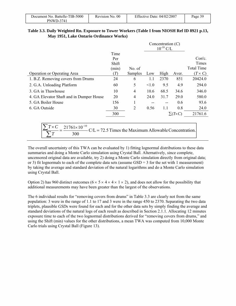
Table 3.3 shows a time-weighted average “Rn. Exposure” to tower workers at the Lake Ontario Ordinance Works (LOOW) where high-226Ra content K-65 tailings were stored (NIOSH SQRI Ref ID 8921, pp. 13-14 of .pdf, R.C. Heatherton to W.B. Harris, 18 May 1951). Study of this and related documents shows that these measurements represent “equilibrium-equivalent radon concentrations” as defined by ICRP publications 32 and 65. Thus, 10−10 Ci/L represents 100 pCi/L or 1 working level (WL) if an equilibrium factor of 1.00 is assumed.
This TWA covers a shift in which the worker was exposed for 300 minutes (5 hours). The author of this report states, “tower operations might show life time variations on any day from the estimated average times assigned to teach operation or operating area in Table I. The error inherent in this fact would probably far outweight (sic) any sampling or measurement error.”
Document No. Battelle-TIB-5000 PNWD-3741
Revision No. 00 Effective Date: 04/02/2007 Page 39
Table 3.3. Daily Weighted Rn. Exposure to Tower Workers (Table I from NIOSH Ref ID 8921 p.13, May 1951, Lake Ontario Ordinance Works)
Concentration (C) 10-10 C/L
Operation or Operating Area
Time Per
Shift (min) (T)
No. of Samples Low High Aver.
Con'c. Times
Total Time (T × C)
1. B.Z. Removing covers from Drums 24 6 1.1 2370 851 20424.02. G.A. Unloading Platform 60 5 <1.0 9.5 4.9 294.03. GA in Thawhouse 10 4 10.6 68.5 34.6 346.04. GA Elevator Shaft and in Dumper House 20 4 24.0 31.7 29.0 580.05. GA Boiler House 156 1 -- -- 0.6 93.66. GA Outside 30 2 0.56 1.1 0.8 24.0
300 ∑(T×C) 21761.6
The overall uncertainty of this TWA can be evaluated by 1) fitting lognormal distributions to these data summaries and doing a Monte Carlo simulation using Crystal Ball. Alternatively, since complete, uncensored original data are available, try 2) doing a Monte Carlo simulation directly from original data; or 3) fit lognormals to each of the complete data sets (assume GSD = 3 for the set with 1 measurement) by taking the average and standard deviation of the natural logarithms and do a Monte Carlo simulation using Crystal Ball.
Option 2) has 960 distinct outcomes (6 × 5 × 4 × 4 × 1 × 2), and does not allow for the possibility that additional measurements may have been greater than the largest of the observations.
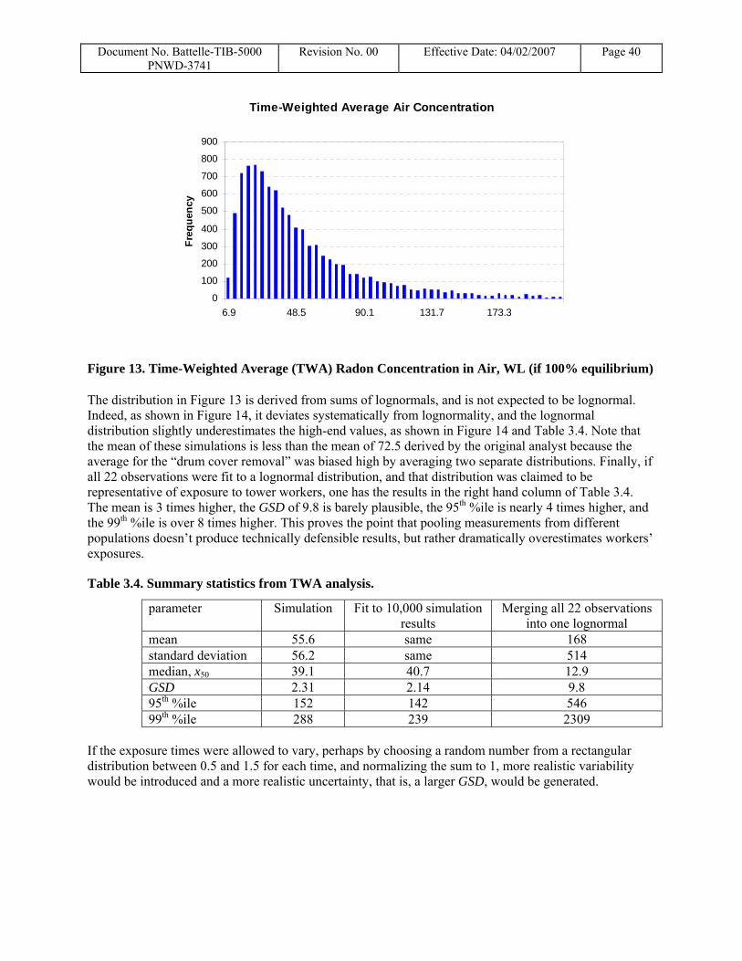
The 6 individual results for “removing covers from drums” in Table 3.3 are clearly not from the same population: 3 were in the range of 1.1 to 17 and 3 were in the range 450 to 2370. Separating the two data triplets, plausible GSDs were found for each and for the other data sets by simply finding the average and standard deviations of the natural logs of each result as described in Section 2.1.1. Allocating 12 minutes exposure time to each of the two lognormal distributions derived for “removing covers from drums,” and using the Shift (min) values for the other distributions, a mean TWA was computed from 10,000 Monte Carlo trials using Crystal Ball (Figure 13).
ion.Concentrat Allowable Maximum theTimes 5.72 C/L 300
1021761 10
=×
=× −
∑∑
TCT
Document No. Battelle-TIB-5000 PNWD-3741
Revision No. 00 Effective Date: 04/02/2007 Page 40
Time-Weighted Average Air Concentration
0
100
200
300
400
500
600
700
800
900
6.9 48.5 90.1 131.7 173.3
Freq
uenc
y
Figure 13. Time-Weighted Average (TWA) Radon Concentration in Air, WL (if 100% equilibrium)
The distribution in Figure 13 is derived from sums of lognormals, and is not expected to be lognormal. Indeed, as shown in Figure 14, it deviates systematically from lognormality, and the lognormal distribution slightly underestimates the high-end values, as shown in Figure 14 and Table 3.4. Note that the mean of these simulations is less than the mean of 72.5 derived by the original analyst because the average for the “drum cover removal” was biased high by averaging two separate distributions. Finally, if all 22 observations were fit to a lognormal distribution, and that distribution was claimed to be representative of exposure to tower workers, one has the results in the right hand column of Table 3.4. The mean is 3 times higher, the GSD of 9.8 is barely plausible, the 95th %ile is nearly 4 times higher, and the 99th %ile is over 8 times higher. This proves the point that pooling measurements from different populations doesn’t produce technically defensible results, but rather dramatically overestimates workers’ exposures.
Table 3.4. Summary statistics from TWA analysis.
parameter Simulation Fit to 10,000 simulation results
Merging all 22 observations into one lognormal
mean 55.6 same 168 standard deviation 56.2 same 514 median, x50 39.1 40.7 12.9 GSD 2.31 2.14 9.8 95th %ile 152 142 546 99th %ile 288 239 2309
If the exposure times were allowed to vary, perhaps by choosing a random number from a rectangular distribution between 0.5 and 1.5 for each time, and normalizing the sum to 1, more realistic variability would be introduced and a more realistic uncertainty, that is, a larger GSD, would be generated.
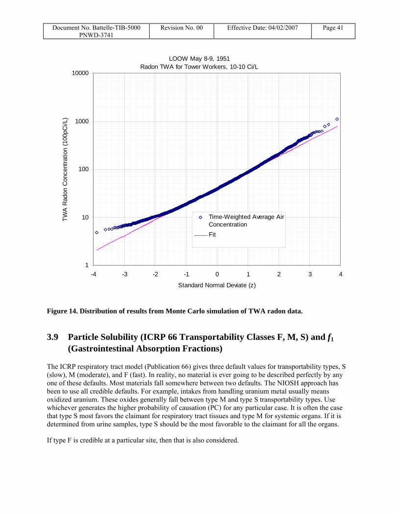
Document No. Battelle-TIB-5000 PNWD-3741
Revision No. 00 Effective Date: 04/02/2007 Page 41
LOOW May 8-9, 1951Radon TWA for Tower Workers, 10-10 Ci/L
1
10
100
1000
10000
-4 -3 -2 -1 0 1 2 3 4
Standard Normal Deviate (z)
TWA
Rad
on C
once
ntra
tion
(100
pCi/L
)
Time-Weighted Average AirConcentrationFit
Figure 14. Distribution of results from Monte Carlo simulation of TWA radon data.
3.9 Particle Solubility (ICRP 66 Transportability Classes F, M, S) and f1 (Gastrointestinal Absorption Fractions)
The ICRP respiratory tract model (Publication 66) gives three default values for transportability types, S (slow), M (moderate), and F (fast). In reality, no material is ever going to be described perfectly by any one of these defaults. Most materials fall somewhere between two defaults. The NIOSH approach has been to use all credible defaults. For example, intakes from handling uranium metal usually means oxidized uranium. These oxides generally fall between type M and type S transportability types. Use whichever generates the higher probability of causation (PC) for any particular case. It is often the case that type S most favors the claimant for respiratory tract tissues and type M for systemic organs. If it is determined from urine samples, type S should be the most favorable to the claimant for all the organs.
If type F is credible at a particular site, then that is also considered.
Document No. Battelle-TIB-5000 PNWD-3741
Revision No. 00 Effective Date: 04/02/2007 Page 42
3.10 Exposure Time and Intake Calculations
In the absence of specific information, assume exposure times as shown in Table 3.5.
Table 3.5. Default exposure time assumptions as a function of date
Dates Default Work
Week Weeks per
Year Hours per
Year 170-hour “Months” per
yeara through 12/31/1950 48 hours 50 2400 14.12
1/1/1951-12/31/1955 44 hours 50 2200 12.94 1/1/1956 onward 40 hours 50 2000 11.76
aFor computing working level months (WLM) from time-weighted average potential alpha energy concentrations of radon or thoron progeny in working levels (WL).
It is important to note that when IMBA performs a dose calculation based on a chronic intake, the intake is assumed to occur 7 days per week, 52.14 (= 365÷7) or 52.29 (= 366÷7) weeks per year. Thus, IMBA’s intake rate in Bq/d should be calculated by dividing the worker’s annual intake rate by 365 (dropping the 0.25 day is favorable to the claimant).
The worker’s annual intake is computed by using
.entration)year)(concper hoursdefault or /h)(actualm2.1( 3annual =I 21
The worker’s chronic daily intake rate for input to IMBA is
.days/year 365(pCi/year)
(pCi/day) annualdaily chronic
II = 22
3.11 Ingestion
In the 1940s and early 1950s, uranium and its compounds seem to have been treated like any other metal and ore, unlike the later decades of the 20th century when it was treated as a radiological hazard. In particular, contamination of the workplace and of workers’ clothing and hands was commonplace and evidently acceptable (Bailey and Rohr 1953b; Bailey and Rohr 1953a; Bailey, Becher, and Henry 1956). Some ingestion intakes are presumed to have occurred, especially among smokers, based on Bailey’s measurements of hand contamination and its transfer to cigarettes (Bailey and Rohr 1953b) and measurements of clothing contamination and its resuspension (Bailey, Becher, and Henry 1956). Some studies have attempted to quantify hand contamination in the workplace (Brouwer, Kroese, and Van Hemmen 1999; Yu and Sherwood 1996). All that is needed for ingestion of contamination is the presence of eating, drinking, smoking, chewing of gum or tobacco, storage or preparation of food, or application of cosmetics without hand washing.
In the interim, ingestion intakes are determined following the OCAS method (Neton 2004).
3.12 Occupational Medical Doses
The default assumptions in OTIB-0006 (Kathren and Shockley 2005) will be used if no other information is available. Photofluorography will be assumed for chest x-rays at du Pont sites for the same years as at Hanford unless information to the contrary is discovered (Gehrmann 1944).

Document No. Battelle-TIB-5000 PNWD-3741
Revision No. 00 Effective Date: 04/02/2007 Page 43
3.13 External Dose Conversion Factors
Correction of radiation survey instrument readings, dosimeter readings, and conversion of recorded neutron doses to correct neutron doses using a wR/Q ratio will be determined using existing OTIBs and IG-001 (Office of Compensation Analysis and Support (OCAS) 2002a).
3.14 External Missed Dose When There Was Monitoring
“Missed” doses are assigned for zero, “minimal,” or null dosimeter results readings to account doses below the “limit of detection” (LOD) being received by a monitored worker but not recorded or reported (Office of Compensation Analysis and Support (OCAS) 2002a). Missed dose can also be assigned for a lost or damaged dosimeter.
One approach is to use co-worker data following the methods of Merwin (2005). In this case, the worker is assigned the same dose as a worker with a similar job title for the period in question, assuming that the co-worker’s dose is a mean value. The imputed dose is taken as a lognormal distribution with a median (IREP Parameter 1) = (Appropriate Coworker’s Dose) × 0.5469 (= exp(−ln2(3)/2)) and a GSD (IREP Parameter 2) = 3. Correcting the Appropriate Coworker’s Dose by the median-to-mean ratio preserves the arithmetic mean (average) value. If the coworker’s dose is the median of a lognormal distribution, then it is used directly as IREP Parameter 1.
Another approach is to substitute a value for each dosimeter reading. The approach here is to assign a triangular distribution with minimum = 0, mode = 0.5×LOD, and maximum = LOD.
3.15 Internal Missed Dose When There Was Monitoring
[Reserved]
3.16 Environmental Dose
At uranium plants, environmental dose from five sources is to be evaluated:
• Submersion in a cloud of a radioactive gas or aerosol
• Direct irradiation from a contaminated surface
• Inhalation of a radioactive gas or aerosol
• Irradiation of hands and forearms from contaminated surfaces
• Irradiation of the skin of the whole body.
3.17 Radon and Thoron and Their Short-lived Decay Products
In general, the practices described by Daer et al. (2006) will be followed. Some of what follows is borrowed verbatim from the DOE Standard for Internal Dosimetry (U.S. Department of Energy (DOE) 1999).
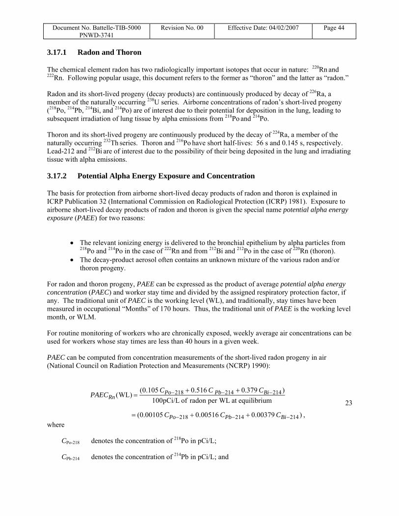
Document No. Battelle-TIB-5000 PNWD-3741
Revision No. 00 Effective Date: 04/02/2007 Page 44
3.17.1 Radon and Thoron
The chemical element radon has two radiologically important isotopes that occur in nature: 220Rn and 222Rn. Following popular usage, this document refers to the former as “thoron” and the latter as “radon.”
Radon and its short-lived progeny (decay products) are continuously produced by decay of 226Ra, a member of the naturally occurring 238U series. Airborne concentrations of radon’s short-lived progeny (218Po, 214Pb, 214Bi, and 214Po) are of interest due to their potential for deposition in the lung, leading to subsequent irradiation of lung tissue by alpha emissions from 218Po and 214Po.
Thoron and its short-lived progeny are continuously produced by the decay of 224Ra, a member of the naturally occurring 232Th series. Thoron and 216Po have short half-lives: 56 s and 0.145 s, respectively. Lead-212 and 212Bi are of interest due to the possibility of their being deposited in the lung and irradiating tissue with alpha emissions.
3.17.2 Potential Alpha Energy Exposure and Concentration
The basis for protection from airborne short-lived decay products of radon and thoron is explained in ICRP Publication 32 (International Commission on Radiological Protection (ICRP) 1981). Exposure to airborne short-lived decay products of radon and thoron is given the special name potential alpha energy exposure (PAEE) for two reasons:
• The relevant ionizing energy is delivered to the bronchial epithelium by alpha particles from
218Po and 214Po in the case of 222Rn and from 212Bi and 212Po in the case of 220Rn (thoron). • The decay-product aerosol often contains an unknown mixture of the various radon and/or
thoron progeny.
For radon and thoron progeny, PAEE can be expressed as the product of average potential alpha energy concentration (PAEC) and worker stay time and divided by the assigned respiratory protection factor, if any. The traditional unit of PAEC is the working level (WL), and traditionally, stay times have been measured in occupational “Months” of 170 hours. Thus, the traditional unit of PAEE is the working level month, or WLM.
For routine monitoring of workers who are chronically exposed, weekly average air concentrations can be used for workers whose stay times are less than 40 hours in a given week.
PAEC can be computed from concentration measurements of the short-lived radon progeny in air (National Council on Radiation Protection and Measurements (NCRP) 1990):
218 214 214
218 214 214
(0.105 0.516 0.379 )(WL)
100pCi/L of radon per WL at equilibrium
(0.00105 0.00516 0.00379 ) ,
Po Pb BiRn
Po Pb Bi
C C CPAEC
C C C
− − −
− − −
+ +=
= + + 23
where
CPo-218 denotes the concentration of 218Po in pCi/L;
CPb-214 denotes the concentration of 214Pb in pCi/L; and

Document No. Battelle-TIB-5000 PNWD-3741
Revision No. 00 Effective Date: 04/02/2007 Page 45
CBi-214 denotes the concentration of 214Bi in pCi/L. PAEC can be computed from concentration measurements of the short-lived thoron progeny in air (United Nations Scientific Committee on the Effects of Atomic Radiation (UNSCEAR) 1993):
( )
( )
Pb-212 212
212 212
0.913 0.087(WL)
7.43pCi/L of thoron per WL at Equilibrium
0.12288 0.011709 ,
BiTn
Pb Bi
C CPAEC
C C
−
− −
+=
= +
24
where
CPb-212 denotes the concentration of 212Po in pCi/L; and
CBi-212 denotes the concentration of 212Bi in pCi/L.
3.17.3 Equilibrium Factors
When radon and thoron concentration measurements are given, equilibrium factors are needed to convert these to potential alpha energy concentrations (PAEC) in working levels (WL). Another acceptable method for workplace monitoring of exposure to radon progeny is to measure the 222Rn itself, and convert it to PAEC using known equilibrium factors. One may calculate equilibrium equivalent concentration, EEC, from radon concentration measurements, C, based on knowledge or assumption of an equilibrium factor, F:
FCEEC ⋅= )pCi/L()pCi/L( 25
If F has not been measured, it is acceptable under some circumstances to assume a default indoor value of FRn = 0.4 (International Commission on Radiological Protection (ICRP) 1993; United Nations Scientific Committee on the Effects of Atomic Radiation (UNSCEAR) 1988; United Nations Scientific Committee on the Effects of Atomic Radiation (UNSCEAR) 1993). If C is in units of μCi/mL, then EEC will also be in units of μCi/mL (note: 1 pCi/L = 10-9 μCi/mL).
For 222Rn, FRn is defined as:
222
214214218 379.0516.0105.0
−
−−− ++=
Rn
BiPbPbRn C
CCCF 26
where
CPo-218 = the concentration of 218Po;
CPb-214 = the concentration of 214Pb
CBi-214 = the concentration of 214Bi; and
CRn-222 = the concentration of 222Rn.
For 220Rn, FTn is defined as
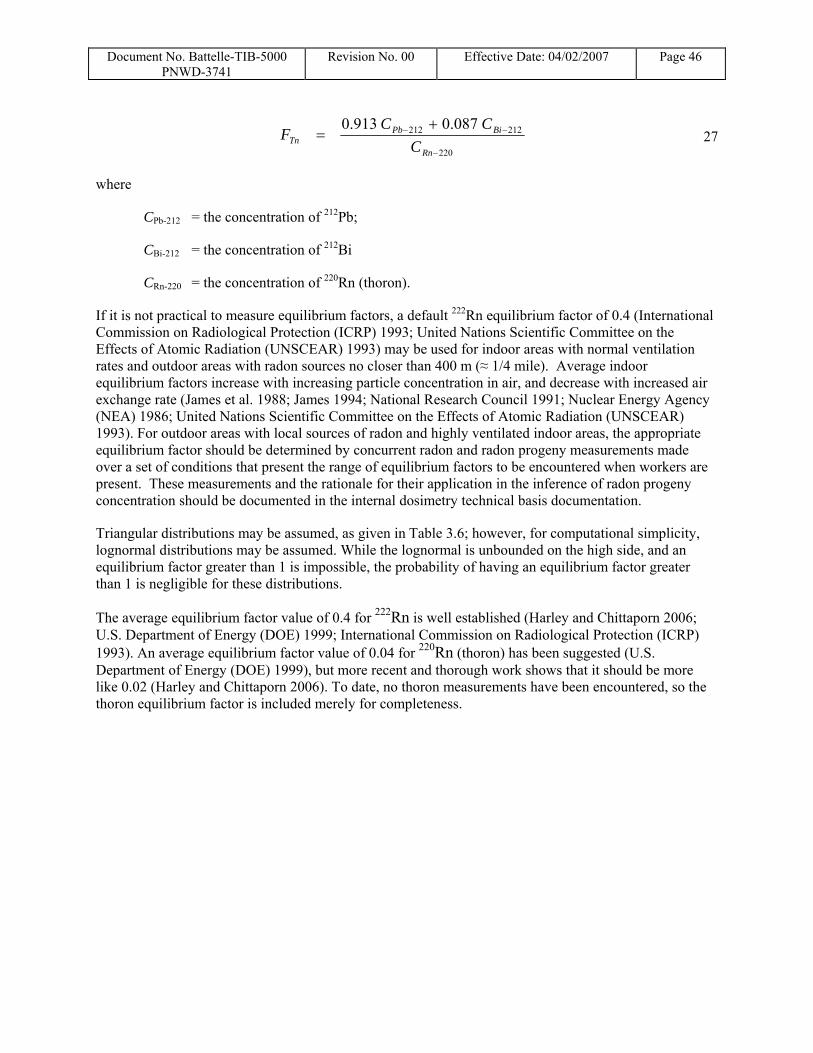
Document No. Battelle-TIB-5000 PNWD-3741
Revision No. 00 Effective Date: 04/02/2007 Page 46
220
212212 087.0913.0
−
−− +=
Rn
BiPbTn C
CCF 27
where
CPb-212 = the concentration of 212Pb;
CBi-212 = the concentration of 212Bi
CRn-220 = the concentration of 220Rn (thoron).
If it is not practical to measure equilibrium factors, a default 222Rn equilibrium factor of 0.4 (International Commission on Radiological Protection (ICRP) 1993; United Nations Scientific Committee on the Effects of Atomic Radiation (UNSCEAR) 1993) may be used for indoor areas with normal ventilation rates and outdoor areas with radon sources no closer than 400 m (≈ 1/4 mile). Average indoor equilibrium factors increase with increasing particle concentration in air, and decrease with increased air exchange rate (James et al. 1988; James 1994; National Research Council 1991; Nuclear Energy Agency (NEA) 1986; United Nations Scientific Committee on the Effects of Atomic Radiation (UNSCEAR) 1993). For outdoor areas with local sources of radon and highly ventilated indoor areas, the appropriate equilibrium factor should be determined by concurrent radon and radon progeny measurements made over a set of conditions that present the range of equilibrium factors to be encountered when workers are present. These measurements and the rationale for their application in the inference of radon progeny concentration should be documented in the internal dosimetry technical basis documentation.
Triangular distributions may be assumed, as given in Table 3.6; however, for computational simplicity, lognormal distributions may be assumed. While the lognormal is unbounded on the high side, and an equilibrium factor greater than 1 is impossible, the probability of having an equilibrium factor greater than 1 is negligible for these distributions.
The average equilibrium factor value of 0.4 for 222Rn is well established (Harley and Chittaporn 2006; U.S. Department of Energy (DOE) 1999; International Commission on Radiological Protection (ICRP) 1993). An average equilibrium factor value of 0.04 for 220Rn (thoron) has been suggested (U.S. Department of Energy (DOE) 1999), but more recent and thorough work shows that it should be more like 0.02 (Harley and Chittaporn 2006). To date, no thoron measurements have been encountered, so the thoron equilibrium factor is included merely for completeness.
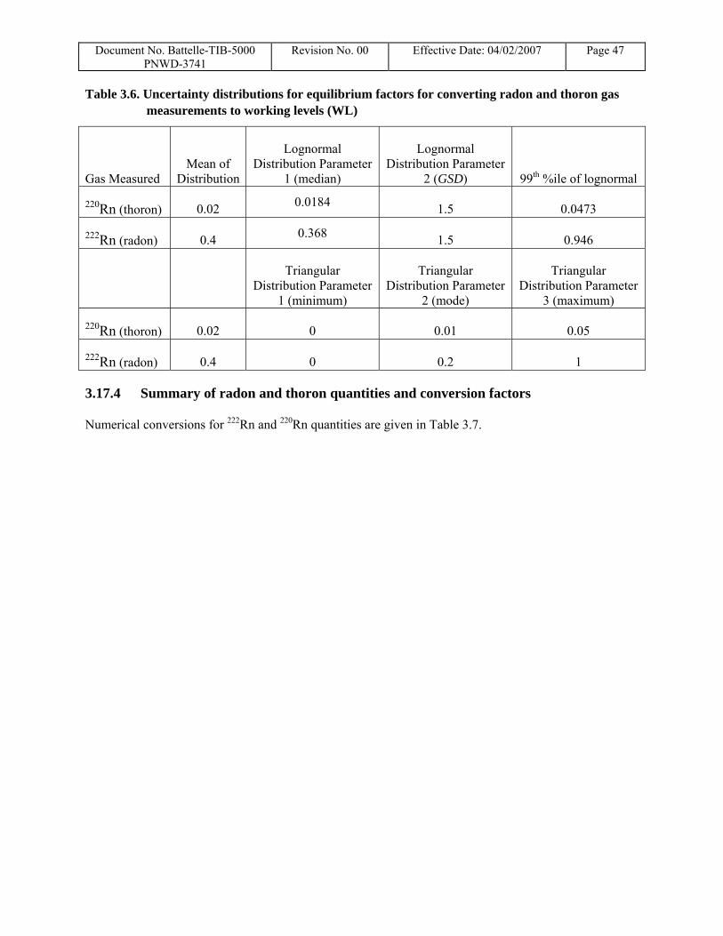
Document No. Battelle-TIB-5000 PNWD-3741
Revision No. 00 Effective Date: 04/02/2007 Page 47
Table 3.6. Uncertainty distributions for equilibrium factors for converting radon and thoron gas measurements to working levels (WL)
Gas Measured Mean of
Distribution
Lognormal Distribution Parameter
1 (median)
Lognormal Distribution Parameter
2 (GSD) 99th %ile of lognormal
220Rn (thoron) 0.02 0.0184 1.5 0.0473
222Rn (radon) 0.4 0.368 1.5 0.946
Triangular
Distribution Parameter 1 (minimum)
Triangular Distribution Parameter
2 (mode)
Triangular Distribution Parameter
3 (maximum)
220Rn (thoron) 0.02 0 0.01 0.05
222Rn (radon) 0.4 0 0.2 1
3.17.4 Summary of radon and thoron quantities and conversion factors
Numerical conversions for 222Rn and 220Rn quantities are given in Table 3.7.

Document No. Battelle-TIB-5000 PNWD-3741
Revision No. 00 Effective Date: 04/02/2007 Page 48
Table 3.7. Summary of numerical conversions for radon and thoron quantities, regardless of the precision of measurements
Multiply In Units
Of By To Obtain In Units
Of
Concentration, C pCi/L 10−9 Concentration, C μCi/mL
Ambient 222Rn or 220Rn concentration, C
pCi/L F* Equilibrium equivalent 222Rn or 220Rn concentration, EEC
pCi/L
222Rn EEC pCi/L 1/100 = 0.01 Potential alpha energy concentration, PAEC
WL
220Rn EEC pCi/L 1/(7.43) = 0.13459 PAEC WL
222Rn or 220Rn progeny PAEC WL Exposure time, t (hours) ÷170
Potential alpha energy exposure, PAEE
WLM
Integrated 222Rn concentration, NV (ambient)
pCi·d/L F× 1.4118E-3 PAEE WLM
Integrated 222Rn concentration, NV (ambient)
pCi·d/L 5.6471E-4 assuming F= 0.4
PAEE WLM
PAEC WLM 4.2490E-3 Potential alpha energy intake, I, of 222Rn or 220Rn progeny
J
*For 222Rn, Fdefault= 0.4; for 220Rn, Fdefault= 0.02
3.18 Radium Monitoring by Breath Radon Analysis
The measurement of 222Rn in breath as a bioassay for 226Ra was pioneered by Evans (Evans 1943) and by Harley of the AEC Health and Safety Laboratory (HASL) (Harley, Jetter, and Eisenbud 1951), and breath measurements were conducted by HASL personnel. Evans found that 1 pCi/L of 222Rn in exhaled breath indicated the presence of 0.1 µg (0.0989 µCi) of 226Ra in the body (Evans 1943). However, Stabin calculated that 1 pCi/L of 222Rn in exhaled breath indicated the presence of 0.252 µCi of 226Ra in the body (Stabin 2005). The latter value is more favorable to the claimant and will be used in this work.
3.19 Determination of the Uncertainty Distribution for Annual Organ Doses Summed Over Multiple Intakes
Assumptions favorable to the claimant are needed regarding the uncertainty distribution and uncertainty parameters for annual doses from intakes in all prior years.
Document No. Battelle-TIB-5000 PNWD-3741
Revision No. 00 Effective Date: 04/02/2007 Page 49
When any uncertain variables described by distributions are added, their variances are added. For Normal distributions, this results in a straightforward means of determining the sum and its uncertainty, since the sum of Normally-distributed variables is Normally-distributed. For lognormal distributions, the product is lognormally-distributed, but the sum has no analytical distribution. This can be explored using Monte Carlo simulations.
One defensible workaround would be to sum the arithmetic mean annual doses received in each year from intakes in all prior years, and sum their variances. Then the resulting sum could be deemed to be lognormally distributed with a mean equal to the sum of mean annual doses and a variance equal to the sum of the variances of the mean annual doses. This approximation may be good enough to be defensible, but it will need to be tested using Monte Carlo simulations.
There is also the problem of uncertainty correlations across years4. For external doses, uncertainties from one year to another will be somewhat correlated (for example, if there were systematic errors in dosimeter calibration) and somewhat uncorrelated due to random fluctuations. For annual doses from intakes of tenaciously-retained radionuclides, uncertainties are correlated with r2 ~ 1.
Suppose an individual had an intake in 1950 for which we estimate a median and GSD, say x50 = 1 and GSD = 3. We use IMBA to calculate annual doses from the median value. Thus, if IREP picks, say, the 80th %ile of the annual dose in 1950 for the intake in 1950, it should pick the 80th %ile of the annual doses for all subsequent years due to this intake. For the annual dose in 1951 due to the intake in 1950, the 80th %ile should be chosen. For the annual dose in 1951 due to an intake in 1951, IREP may pick, say, the 25th %ile. It should then pick the same percentile of each annual dose distribution due to the 1951 intake.
Using correlated uncertainties would result in broader dose distributions and larger PC values. Even external doses should have some degree of correlation because 1) systematic dosimetry calibration or response errors would correlate from year to year; and 2) an individual’s behavioral differences from some average would differ from year to year, e.g., his or her job may have required facing toward the source of radiation more than was assumed and this would be the same from one year to the next as long as the individual had the same job.
Conclusions drawn from Monte Carlo simulations of the sum of random variables drawn from lognormal distributions with the same GSD:
1. The arithmetic mean of the resultant sum is equal to the sum of the arithmetic means of the random variables.
4 While the correlated uncertainties here contain components of both bias and uncertainty, the bias component is an unknown bias. According to the ISO and NIST, such uncertainties, termed Type B uncertainties, are treated mathematically the same as random uncertainties (International Organization for Standardization (ISO) 1995; Taylor and Kuyatt 1994). The ISO and NIST chose to use the terminology “Type A” uncertainties (“those which are evaluated by statistical methods”, or “component of uncertainty arising from a random effect,”) and “Type B” uncertainties (“those which are evaluated by other means,” or “component of uncertainty arising from a systematic effect”). “There is not always a simple correspondence between the classification of uncertainty components into categories A and B and the commonly used classification of uncertainty components as “random” and “systematic.” The nature of an uncertainty component is conditioned by the use made of the corresponding quantity, that is, on how that quantity appears in the mathematical model that describes the measurement process. When the corresponding quantity is used in a different way, a “random” component may become a “systematic” component and vice versa. Thus the terms “random uncertainty” and “systematic uncertainty” can be misleading when generally applied. If the bias were known, it would be corrected for (with perhaps an uncertain correction factor).
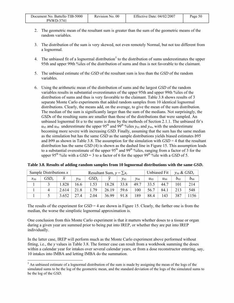
Document No. Battelle-TIB-5000 PNWD-3741
Revision No. 00 Effective Date: 04/02/2007 Page 50
2. The geometric mean of the resultant sum is greater than the sum of the geometric means of the random variables.
3. The distribution of the sum is very skewed, not even remotely Normal, but not too different from a lognormal.
4. The unbiased fit of a lognormal distribution5 to the distribution of sums underestimates the upper 95th and upper 99th %iles of the distribution of sums and thus is not favorable to the claimant.
5. The unbiased estimate of the GSD of the resultant sum is less than the GSD of the random variables.
6. Using the arithmetic mean of the distribution of sums and the largest GSD of the random variables results in substantial overestimates of the upper 95th and upper 99th %iles of the distribution of sums and thus is very favorable to the claimant. Table 3.8 shows results of 3 separate Monte Carlo experiments that added random samples from 10 identical lognormal distributions. Clearly, the means add, on the average, to give the mean of the sum distribution. The median of the sum is significantly larger than the sum of the medians. Not surprisingly, the GSDs of the resulting sums are smaller than those of the distributions that were sampled. An unbiased lognormal fit u to the sums is done by the methods of Section 2.1.1. The unbiased fit’s u95 and u99 underestimate the upper 95th and 99th %iles y95 and y99, with the underestimate becoming more severe with increasing GSD. Finally, assuming that the sum has the same median as the simulation but has the same GSD as the sample distributions yields biased estimates b95 and b99 as shown in Table 3.8. The assumption for the simulation with GSD = 4 that the resultant distribution has the same GSD (4) is shown as the dashed line in Figure 15. This assumption leads to a substantial overestimate of the upper 95th and 99th %iles, ranging from a factor of 3 for the upper 95th %ile with a GSD = 3 to a factor of 6 for the upper 99th %ile with a GSD of 5.
Table 3.8. Results of adding random samples from 10 lognormal distributions with the same GSD.
The results of the experiment for GSD = 4 are shown in Figure 15. Clearly, the farther one is from the median, the worse the simplistic lognormal approximation is.
One conclusion from this Monte Carlo experiment is that it matters whether doses to a tissue or organ during a given year are summed prior to being put into IREP, or whether they are put into IREP individually.
In the latter case, IREP will perform much as the Monte Carlo experiment above performed without fitting, i.e., the y values in Table 3.8. The former case can result from a workbook summing the doses within a calendar year for intakes over several calendar years, or from a dose reconstructor entering, say, 10 intakes into IMBA and letting IMBA do the summation. 5 An unbiased estimate of a lognormal distribution of the sum is made by assigning the mean of the logs of the simulated sums to be the log of the geometric mean, and the standard deviation of the logs of the simulated sums to be the log of the GSD.
Sample Distributions x Resultant Sum, y = ∑xi Unbiased Fit y50 & GSDx x50 GSDx x y50 GSDy y y95 y99 u95 u99 b95 b99 1 3 1.828 16.6 1.53 18.28 33.8 49.7 33.5 44.7 101 214 1 4 2.614 21.8 1.79 26.19 59.6 100 56.7 84.1 213 548 1 5 3.652 27.4 2.04 36.99 91.8 189 88.4 143 387 1156

Document No. Battelle-TIB-5000 PNWD-3741
Revision No. 00 Effective Date: 04/02/2007 Page 51
If the summation is done prior to inputting the sum into IREP, then the means of the various doses should be added (not the medians or modes) to get an unbiased estimate of the resultant mean. If one simply added the medians (= 1 in this case) of the initial distributions, one would use a median 10 × 1 = 10, while the medians of the Monte Carlo experiment shown in Table 3.8 were 16.6, 21.8, and 27.4, respectively, for GSDs of 3, 4, and 5. For this experiment, assuming a median of 10 is 60.2%, 45.9%, and 36.5%, respectively, of the actual medians for GSDs of 3, 4, and 5.
The GSD of the resultant sum is significantly less than the GSDs of the distributions that were summed. It is not clear what the GSD would be if the initial distributions had varying medians and varying GSDs. If there is a positive correlation among the doses being summed, the assumption that the GSD of the sum is equal to the largest GSD of any of the input distributions may not result in much of an overestimate at the 95th and 99th %iles of dose.
Figure 15. Graph of 10,000 Monte Carlo trials adding 10 samples from lognormal distributions with x50 = 1 and GSD = 4.
The geometric mean is needed as an input parameter to IREP. If the means of the input dose distributions were summed, the geometric mean would have to be determined from the correct mean and the overestimated GSD. For the first line in Table 3.8, the sum of the means (18.28) would be multiplied by 0.5469 (using a GSD of 3) to get the median of 9.997. Doing the same for the other lines in Table 3.8 gives a similar answer of 10. That is the same answer one gets if one simply adds the medians of the original distributions. Summing the medians and using the highest GSD of the individual distributions will produce a smaller overestimate than indicated by the Monte Carlo experiment, since the geometric mean is underestimated.
A policy of simply adding the medians of the lognormally distributed doses and using the highest GSD from the doses that were summed is chosen here because it is favorable to the claimant and technically feasible.
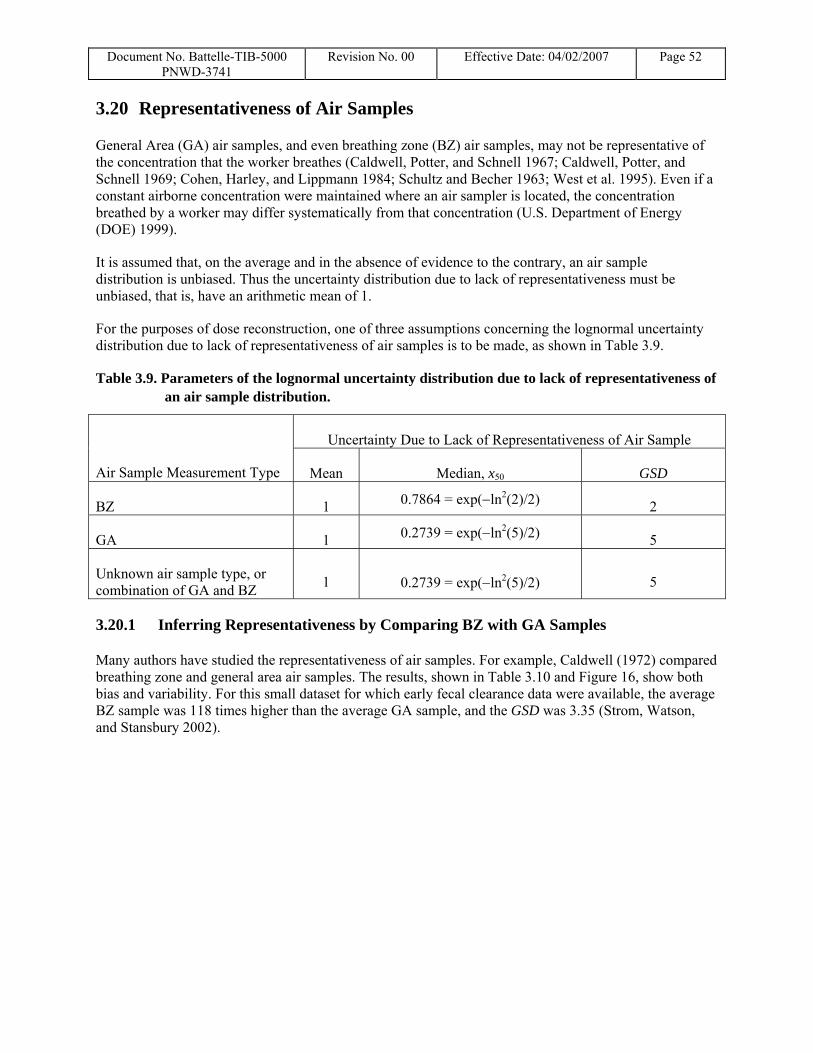
Document No. Battelle-TIB-5000 PNWD-3741
Revision No. 00 Effective Date: 04/02/2007 Page 52
3.20 Representativeness of Air Samples
General Area (GA) air samples, and even breathing zone (BZ) air samples, may not be representative of the concentration that the worker breathes (Caldwell, Potter, and Schnell 1967; Caldwell, Potter, and Schnell 1969; Cohen, Harley, and Lippmann 1984; Schultz and Becher 1963; West et al. 1995). Even if a constant airborne concentration were maintained where an air sampler is located, the concentration breathed by a worker may differ systematically from that concentration (U.S. Department of Energy (DOE) 1999).
It is assumed that, on the average and in the absence of evidence to the contrary, an air sample distribution is unbiased. Thus the uncertainty distribution due to lack of representativeness must be unbiased, that is, have an arithmetic mean of 1.
For the purposes of dose reconstruction, one of three assumptions concerning the lognormal uncertainty distribution due to lack of representativeness of air samples is to be made, as shown in Table 3.9.
Table 3.9. Parameters of the lognormal uncertainty distribution due to lack of representativeness of an air sample distribution.
Uncertainty Due to Lack of Representativeness of Air Sample
Air Sample Measurement Type Mean Median, x50 GSD
BZ 1 0.7864 = exp(−ln2(2)/2) 2
GA 1 0.2739 = exp(−ln2(5)/2) 5
Unknown air sample type, or combination of GA and BZ 1 0.2739 = exp(−ln2(5)/2) 5
3.20.1 Inferring Representativeness by Comparing BZ with GA Samples
Many authors have studied the representativeness of air samples. For example, Caldwell (1972) compared breathing zone and general area air samples. The results, shown in Table 3.10 and Figure 16, show both bias and variability. For this small dataset for which early fecal clearance data were available, the average BZ sample was 118 times higher than the average GA sample, and the GSD was 3.35 (Strom, Watson, and Stansbury 2002).

Document No. Battelle-TIB-5000 PNWD-3741
Revision No. 00 Effective Date: 04/02/2007 Page 53
Table 3.10. Breathing zone (BZ or Lapel) air sampling and general area (GA) air sampling (data digitized from Caldwell 1972; adapted from (Strom, Watson, and Stansbury 2002)).
General Area (Bq m−3)
Lapel (Bq m−3) Ratio Lapel/GA
0.2 3 14.5 0.22 4.7 21.1 0.18 14 79.2 1.62 28 17.5 0.24 19 79.2 0.35 161 458 0.65 72 110 0.45 72 160
Average 118 Standard Deviation 147
Coefficient of Variation 1.25 Geometric Mean 63.7
Geometric Standard Deviation 3.35 Minimum 14.5 Maximum 458
Number 8
Figure 16. Graph from Caldwell (1972) digitized in Table 3.10. The straight line refers to predictions of the ICRP Publication 2 lung model
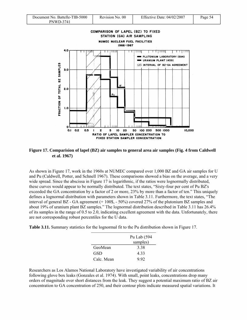
Document No. Battelle-TIB-5000 PNWD-3741
Revision No. 00 Effective Date: 04/02/2007 Page 54
Figure 17. Comparision of lapel (BZ) air samples to general area air samples (Fig. 4 from Caldwell et al. 1967)
As shown in Figure 17, work in the 1960s at NUMEC compared over 1,000 BZ and GA air samples for U and Pu (Caldwell, Potter, and Schnell 1967). These comparisons showed a bias on the average, and a very wide spread. Since the abscissa in Figure 17 is logarithmic, if the ratios were lognormally distributed, these curves would appear to be normally distributed. The text states, “Sixty-four per cent of Pu BZ's exceeded the GA concentration by a factor of 2 or more, 23% by more than a factor of ten.” This uniquely defines a lognormal distribution with parameters shown in Table 3.11. Furthermore, the text states, “The interval of general BZ - GA agreement (+ 100$, - 50%) covered 27% of the plutonium BZ samples and about 19% of uranium plant BZ samples.” The lognormal distribution described in Table 3.11 has 26.4% of its samples in the range of 0.5 to 2.0, indicating excellent agreement with the data. Unfortunately, there are not corresponding robust percentiles for the U data.
Table 3.11. Summary statistics for the lognormal fit to the Pu distribution shown in Figure 17.
Pu Lab (594
samples) GeoMean 3.38 GSD 4.33 Calc. Mean 9.92
Researchers as Los Alamos National Laboratory have investigated variability of air concentrations following glove box leaks (Gonzales et al. 1974). With small, point leaks, concentrations drop many orders of magnitude over short distances from the leak. They suggest a potential maximum ratio of BZ air concentration to GA concentration of 250, and their contour plots indicate measured spatial variations. It
Document No. Battelle-TIB-5000 PNWD-3741
Revision No. 00 Effective Date: 04/02/2007 Page 55
is difficult to deduce the distribution of BZ to GA ratios, but it would appear that the LANL work is consistent with a GSD of 4.1 (~250(1/(2*1.96))) or more, based on the assumption that the range 1 to 250 represents the 2.5 percentile to 97.5 percentile. If GA air samples cannot do better than a GSD of 4.33 in predicting BZ samples, then they should do even worse predicting intakes. But it is necessary to determine how well BZ air samples predict intakes to complete this line of reasoning.
3.20.2 Inferring Representativeness by Comparing Excretion Rates Predicted from Air Samples with Measured Excretion Rates
If bioassay is the gold standard for intakes, then representativeness of air samples can be deduced by comparing predicted urinary excretion rates with measured values. Without regard to bias (that is, systematic differences between biokinetic models and real workers), variability will be due to lack of representativeness of air samples as well as to other factors such as biological variability. However, such data are a start.
Yu and Sherwood (1996) examined the relationships between urinary elimination, airborne concentration, and radioactive hand contamination for workers exposed to uranium. One cannot deduce the variability of an individual air sample and its subsequent urinary excretion value for individual workers, but one can understand average values. Airborne uranium concentration bore a strong, positive correlation with production index, with r2 = 0.73 at p<0.001. Urinary uranium excretion rate can be related to airborne concentration for 20 weekly average measurements of each variable, as shown in Figure 18. These GSDs, in the range of 1.5 to 1.6, are for weekly averages over many workers and many air samples, and thus represent a value much lower than an individual air sample and an individual person. Each of the 20 weekly ratios represents a mean that is much more precisely known than any single ratio.
1
10
-2.5 -2 -1.5 -1 -0.5 0 0.5 1 1.5 2 2.5Standard Normal Deviate, z
Dai
ly U
Exc
retio
n / A
vera
ge A
irbor
neC
onc.
[(µg
/d)/(
µg/m
3 )]
Sorted Dataln(Data) Pred. GM= 2.73 GSD= 1.49Uniform Pred. GM= 2.73 GSD= 1.55Finney Pred. GM= 2.77 GSD= 1.58
Figure 18. Lognormal fit to the ratio of daily uranium excretion divided by the average airborne uranium concentration for maintenance workers, from Yu and Sherwood (1996).
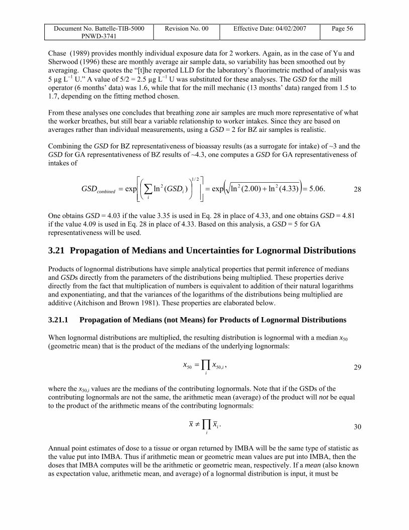
Document No. Battelle-TIB-5000 PNWD-3741
Revision No. 00 Effective Date: 04/02/2007 Page 56
Chase (1989) provides monthly individual exposure data for 2 workers. Again, as in the case of Yu and Sherwood (1996) these are monthly average air sample data, so variability has been smoothed out by averaging. Chase quotes the “[t]he reported LLD for the laboratory’s fluorimetric method of analysis was 5 µg L−1 U.” A value of 5/2 = 2.5 µg L−1 U was substituted for these analyses. The GSD for the mill operator (6 months’ data) was 1.6, while that for the mill mechanic (13 months’ data) ranged from 1.5 to 1.7, depending on the fitting method chosen.
From these analyses one concludes that breathing zone air samples are much more representative of what the worker breathes, but still bear a variable relationship to worker intakes. Since they are based on averages rather than individual measurements, using a GSD = 2 for BZ air samples is realistic.
Combining the GSD for BZ representativeness of bioassay results (as a surrogate for intake) of ~3 and the GSD for GA representativeness of BZ results of ~4.3, one computes a GSD for GA representativeness of intakes of
( ) .06.5)33.4(ln)00.2(lnexp)(lnexp 222/1
2 =+=⎥⎥⎦
⎤
⎢⎢⎣
⎡⎟⎠
⎞⎜⎝
⎛= ∑
iicombined GSDGSD 28
One obtains GSD = 4.03 if the value 3.35 is used in Eq. 28 in place of 4.33, and one obtains GSD = 4.81 if the value 4.09 is used in Eq. 28 in place of 4.33. Based on this analysis, a GSD = 5 for GA representativeness will be used.
3.21 Propagation of Medians and Uncertainties for Lognormal Distributions
Products of lognormal distributions have simple analytical properties that permit inference of medians and GSDs directly from the parameters of the distributions being multiplied. These properties derive directly from the fact that multiplication of numbers is equivalent to addition of their natural logarithms and exponentiating, and that the variances of the logarithms of the distributions being multiplied are additive (Aitchison and Brown 1981). These properties are elaborated below.
3.21.1 Propagation of Medians (not Means) for Products of Lognormal Distributions
When lognormal distributions are multiplied, the resulting distribution is lognormal with a median x50 (geometric mean) that is the product of the medians of the underlying lognormals:
∏=i
ixx ,,5050 29
where the x50,i values are the medians of the contributing lognormals. Note that if the GSDs of the contributing lognormals are not the same, the arithmetic mean (average) of the product will not be equal to the product of the arithmetic means of the contributing lognormals:
∏≠i
ixx . 30
Annual point estimates of dose to a tissue or organ returned by IMBA will be the same type of statistic as the value put into IMBA. Thus if arithmetic mean or geometric mean values are put into IMBA, then the doses that IMBA computes will be the arithmetic or geometric mean, respectively. If a mean (also known as expectation value, arithmetic mean, and average) of a lognormal distribution is input, it must be
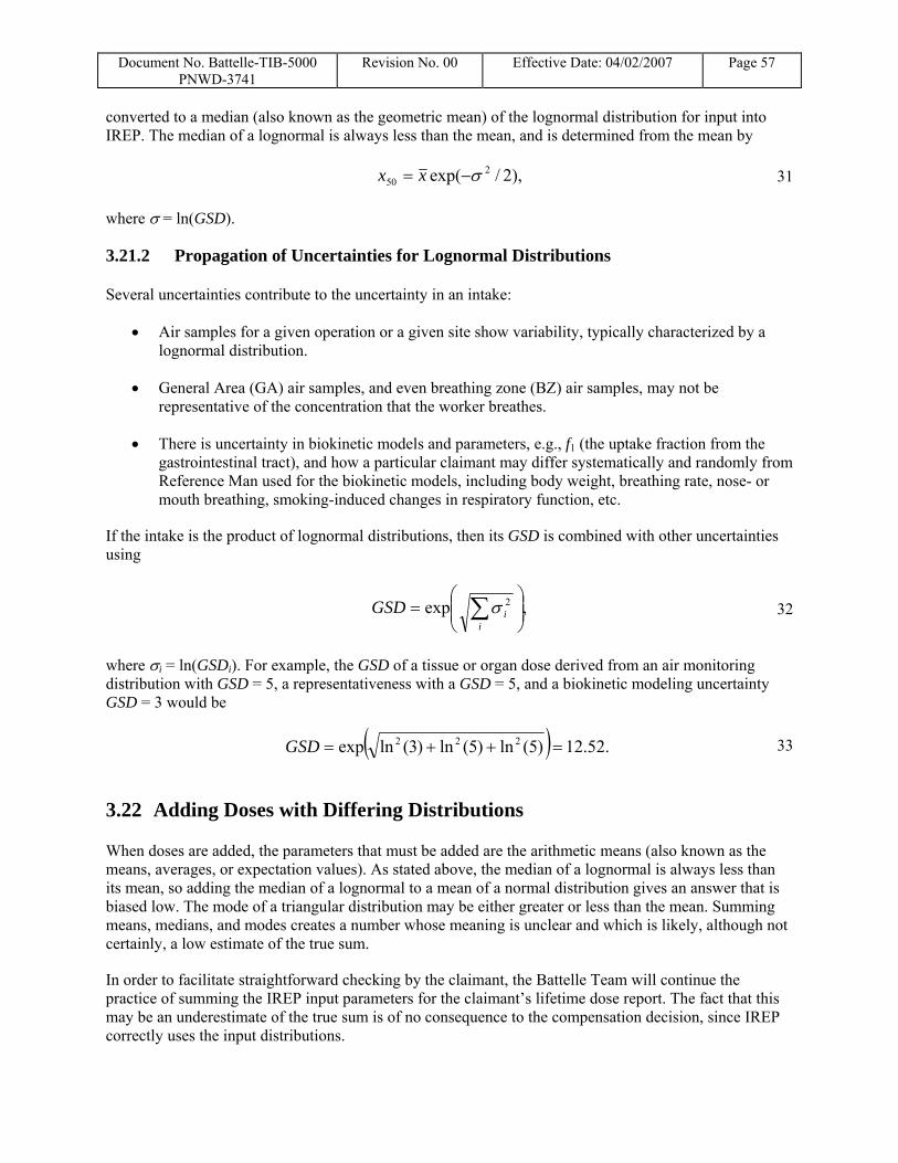
Document No. Battelle-TIB-5000 PNWD-3741
Revision No. 00 Effective Date: 04/02/2007 Page 57
converted to a median (also known as the geometric mean) of the lognormal distribution for input into IREP. The median of a lognormal is always less than the mean, and is determined from the mean by
),2/exp( 250 σ−= xx 31
where σ = ln(GSD).
3.21.2 Propagation of Uncertainties for Lognormal Distributions
Several uncertainties contribute to the uncertainty in an intake:
• Air samples for a given operation or a given site show variability, typically characterized by a lognormal distribution.
• General Area (GA) air samples, and even breathing zone (BZ) air samples, may not be representative of the concentration that the worker breathes.
• There is uncertainty in biokinetic models and parameters, e.g., f1 (the uptake fraction from the gastrointestinal tract), and how a particular claimant may differ systematically and randomly from Reference Man used for the biokinetic models, including body weight, breathing rate, nose- or mouth breathing, smoking-induced changes in respiratory function, etc.
If the intake is the product of lognormal distributions, then its GSD is combined with other uncertainties using
,exp 2⎟⎟⎠
⎞⎜⎜⎝
⎛= ∑
iiGSD σ 32
where σi = ln(GSDi). For example, the GSD of a tissue or organ dose derived from an air monitoring distribution with GSD = 5, a representativeness with a GSD = 5, and a biokinetic modeling uncertainty GSD = 3 would be
( ) .52.12)5(ln)5(ln)3(lnexp 222 =++=GSD 33
3.22 Adding Doses with Differing Distributions
When doses are added, the parameters that must be added are the arithmetic means (also known as the means, averages, or expectation values). As stated above, the median of a lognormal is always less than its mean, so adding the median of a lognormal to a mean of a normal distribution gives an answer that is biased low. The mode of a triangular distribution may be either greater or less than the mean. Summing means, medians, and modes creates a number whose meaning is unclear and which is likely, although not certainly, a low estimate of the true sum.
In order to facilitate straightforward checking by the claimant, the Battelle Team will continue the practice of summing the IREP input parameters for the claimant’s lifetime dose report. The fact that this may be an underestimate of the true sum is of no consequence to the compensation decision, since IREP correctly uses the input distributions.
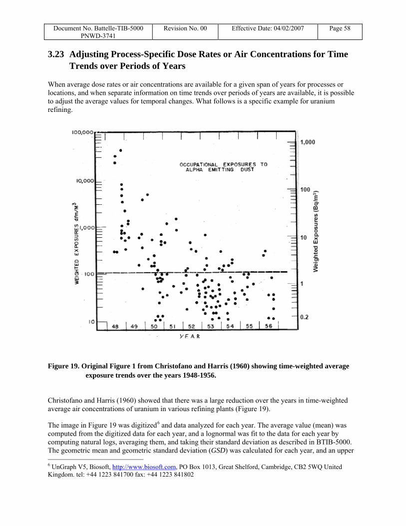
Document No. Battelle-TIB-5000 PNWD-3741
Revision No. 00 Effective Date: 04/02/2007 Page 58
3.23 Adjusting Process-Specific Dose Rates or Air Concentrations for Time Trends over Periods of Years
When average dose rates or air concentrations are available for a given span of years for processes or locations, and when separate information on time trends over periods of years are available, it is possible to adjust the average values for temporal changes. What follows is a specific example for uranium refining.
Figure 19. Original Figure 1 from Christofano and Harris (1960) showing time-weighted average exposure trends over the years 1948-1956.
Christofano and Harris (1960) showed that there was a large reduction over the years in time-weighted average air concentrations of uranium in various refining plants (Figure 19).
The image in Figure 19 was digitized6 and data analyzed for each year. The average value (mean) was computed from the digitized data for each year, and a lognormal was fit to the data for each year by computing natural logs, averaging them, and taking their standard deviation as described in BTIB-5000. The geometric mean and geometric standard deviation (GSD) was calculated for each year, and an upper 6 UnGraph V5, Biosoft, http://www.biosoft.com, PO Box 1013, Great Shelford, Cambridge, CB2 5WQ United Kingdom. tel: +44 1223 841700 fax: +44 1223 841802
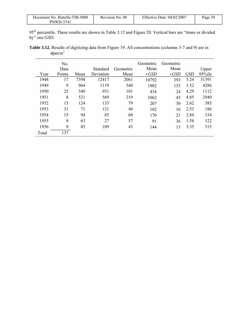
Document No. Battelle-TIB-5000 PNWD-3741
Revision No. 00 Effective Date: 04/02/2007 Page 59
95th percentile. These results are shown in Table 3.12 and Figure 20. Vertical bars are “times or divided by” one GSD.
Table 3.12. Results of digitizing data from Figure 19. All concentrations (columns 3-7 and 9) are in dpm/m3
Year
No. Data
Points Mean Standard
DeviationGeometric
Mean
Geometric Mean ×GSD
Geometric Mean ÷GSD GSD
Upper 95%ile
1948 17 7398 12417 2061 10792 393 5.24 313911949 9 964 1119 540 1902 153 3.52 42861950 25 349 951 101 434 24 4.29 11121951 8 521 569 219 1062 45 4.85 29401952 15 124 133 79 207 30 2.62 3851953 31 71 121 40 102 16 2.53 1861954 15 94 85 60 170 21 2.84 3341955 8 63 27 57 91 36 1.58 1221956 9 85 109 43 144 13 3.35 315
Total 137
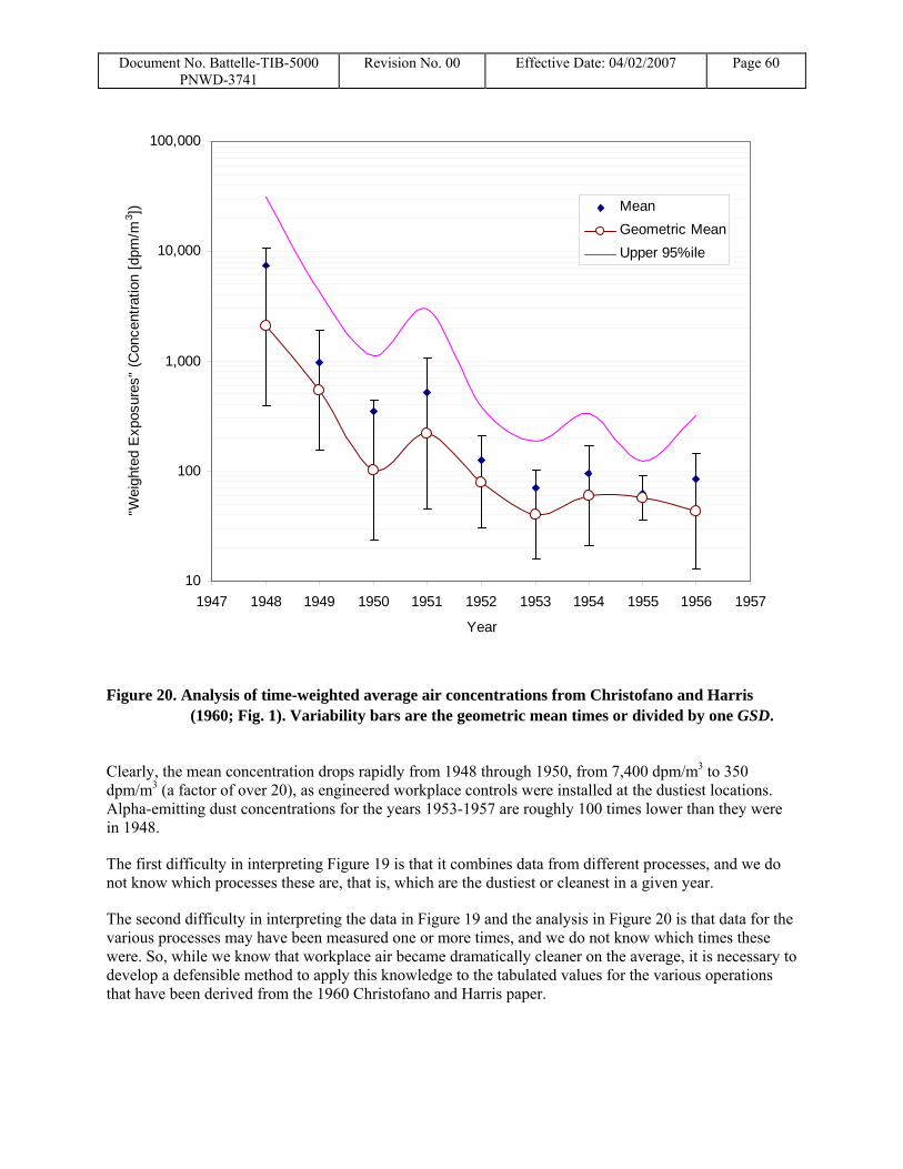
Document No. Battelle-TIB-5000 PNWD-3741
Revision No. 00 Effective Date: 04/02/2007 Page 60
10
100
1,000
10,000
100,000
1947 1948 1949 1950 1951 1952 1953 1954 1955 1956 1957
Year
"Wei
ghte
d E
xpos
ures
" (C
once
ntra
tion
[dpm
/m3 ]) Mean
Geometric MeanUpper 95%ile
Figure 20. Analysis of time-weighted average air concentrations from Christofano and Harris (1960; Fig. 1). Variability bars are the geometric mean times or divided by one GSD.
Clearly, the mean concentration drops rapidly from 1948 through 1950, from 7,400 dpm/m3 to 350 dpm/m3 (a factor of over 20), as engineered workplace controls were installed at the dustiest locations. Alpha-emitting dust concentrations for the years 1953-1957 are roughly 100 times lower than they were in 1948.
The first difficulty in interpreting Figure 19 is that it combines data from different processes, and we do not know which processes these are, that is, which are the dustiest or cleanest in a given year.
The second difficulty in interpreting the data in Figure 19 and the analysis in Figure 20 is that data for the various processes may have been measured one or more times, and we do not know which times these were. So, while we know that workplace air became dramatically cleaner on the average, it is necessary to develop a defensible method to apply this knowledge to the tabulated values for the various operations that have been derived from the 1960 Christofano and Harris paper.
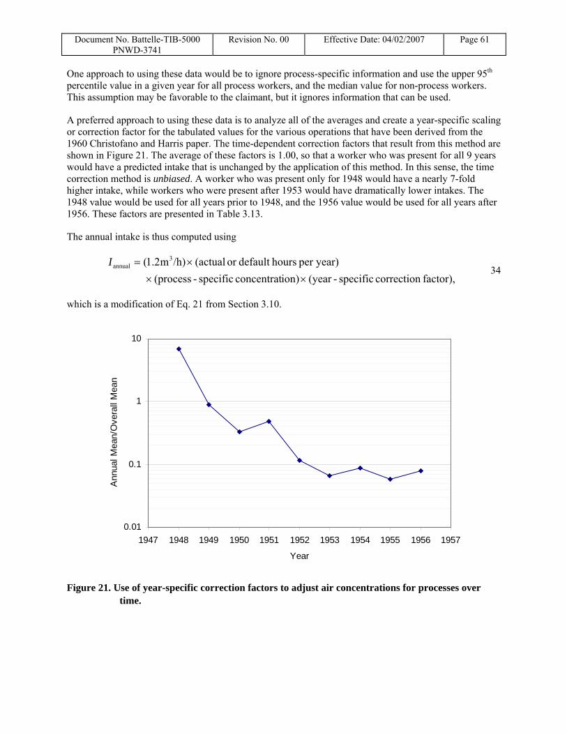
Document No. Battelle-TIB-5000 PNWD-3741
Revision No. 00 Effective Date: 04/02/2007 Page 61
One approach to using these data would be to ignore process-specific information and use the upper 95th percentile value in a given year for all process workers, and the median value for non-process workers. This assumption may be favorable to the claimant, but it ignores information that can be used.
A preferred approach to using these data is to analyze all of the averages and create a year-specific scaling or correction factor for the tabulated values for the various operations that have been derived from the 1960 Christofano and Harris paper. The time-dependent correction factors that result from this method are shown in Figure 21. The average of these factors is 1.00, so that a worker who was present for all 9 years would have a predicted intake that is unchanged by the application of this method. In this sense, the time correction method is unbiased. A worker who was present only for 1948 would have a nearly 7-fold higher intake, while workers who were present after 1953 would have dramatically lower intakes. The 1948 value would be used for all years prior to 1948, and the 1956 value would be used for all years after 1956. These factors are presented in Table 3.13.
The annual intake is thus computed using
factor), correction specific-(year ion)concentrat specific-(process
year)per hoursdefault or (actual /h)m2.1( 3annual
×××=I
34
which is a modification of Eq. 21 from Section 3.10.
0.01
0.1
1
10
1947 1948 1949 1950 1951 1952 1953 1954 1955 1956 1957
Year
Ann
ual M
ean/
Ove
rall
Mea
n
Figure 21. Use of year-specific correction factors to adjust air concentrations for processes over
time.
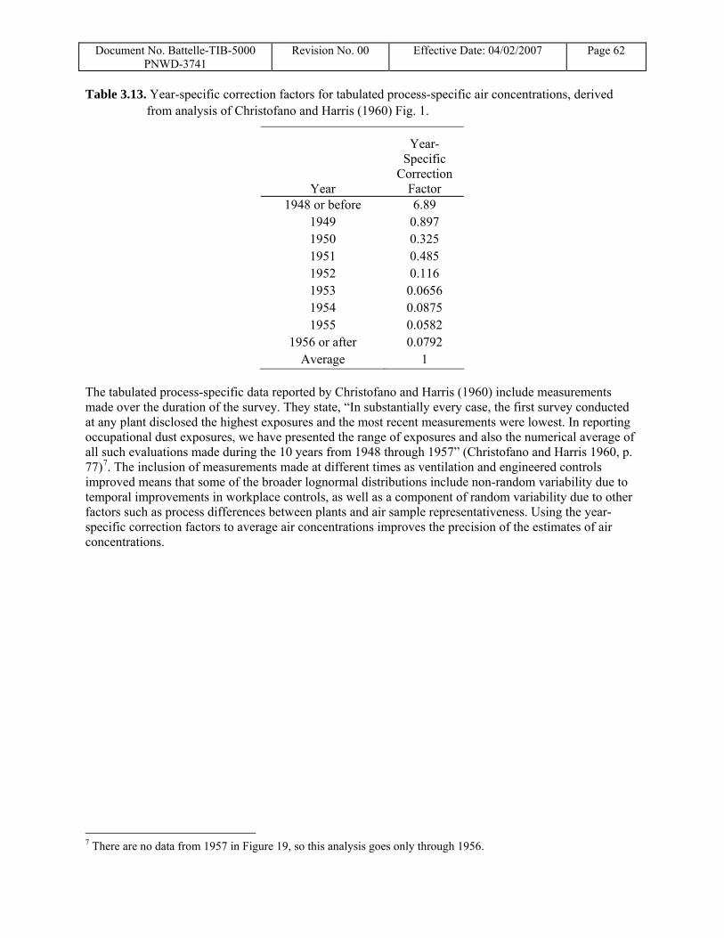
Document No. Battelle-TIB-5000 PNWD-3741
Revision No. 00 Effective Date: 04/02/2007 Page 62
Table 3.13. Year-specific correction factors for tabulated process-specific air concentrations, derived from analysis of Christofano and Harris (1960) Fig. 1.
Year
Year-Specific
Correction Factor
1948 or before 6.89 1949 0.897 1950 0.325 1951 0.485 1952 0.116 1953 0.0656 1954 0.0875 1955 0.0582
1956 or after 0.0792 Average 1
The tabulated process-specific data reported by Christofano and Harris (1960) include measurements made over the duration of the survey. They state, “In substantially every case, the first survey conducted at any plant disclosed the highest exposures and the most recent measurements were lowest. In reporting occupational dust exposures, we have presented the range of exposures and also the numerical average of all such evaluations made during the 10 years from 1948 through 1957” (Christofano and Harris 1960, p. 77)7. The inclusion of measurements made at different times as ventilation and engineered controls improved means that some of the broader lognormal distributions include non-random variability due to temporal improvements in workplace controls, as well as a component of random variability due to other factors such as process differences between plants and air sample representativeness. Using the year-specific correction factors to average air concentrations improves the precision of the estimates of air concentrations.
7 There are no data from 1957 in Figure 19, so this analysis goes only through 1956.
Document No. Battelle-TIB-5000 PNWD-3741
Revision No. 00 Effective Date: 04/02/2007 Page 63
4.0 Glossary
Note: Many of these definitions are borrowed from the DOE Standard on Internal Dosimetry (U.S. Department of Energy (DOE) 1999).
activity median thermodynamic diameter (AMTD): “Fifty percent of the activity (thermodynamically classified) in the aerosol is associated with particles of thermodynamic diameter (dth) greater than the AMTD. A lognormal distribution of particle sizes is usually assumed” (ICRP 1994a).
assigned protection factor (APF): The expected workplace level of respiratory protection that would be provided by a properly functioning respirator or a class of respirators to properly fitted and trained users (ANSI Z88.2-1992). bias: The deviation of a single measured value of a random variable from a corresponding expected value, or a fixed mean deviation from the expected value that remains constant over replicated measurements within the statistical precision of the measurement (synonymous with deterministic error, fixed error, and systematic error) (HPS N13.30-1996). bioassay: Another word for radiobioassay. biokinetic model: A series of often empirically determined mathematical relationships formulated to describe the intake, deposition in respiratory tract (if applicable), uptakes by the transfer compartment from intake compartment(s), uptakes by tissues or organs from the transfer compartment, translocation, retention, and elimination of a radionuclide from the body. censored data: Data that have been recorded as “less than” values rather than the observed numerical values (whether positive, zero, or negative). Class SR-0 gases: Insoluble and nonreactive gases and vapors (ICRP Publication 68, p. x, 1994a). Class SR-1 gases: Soluble or reactive gases and vapors (ICRP Publication 68, p. x, 1994a). Class SR-1 gases: Highly soluble or reactive gases and vapors (ICRP Publication 68, p. x 1994a). compartment: The smallest element in a biokinetic model for which a mathematical representation of a retained quantity is given. Compartments may be organs (e.g., lung, liver), tissues (e.g., bone marrow), or systemic (e.g., the transfer compartment). critical level: Same as decision level. decision level: The amount of a count (LC) or a count rate (LC) or the final instrument measurement of a quantity of analyte (DC or DC ) at or above which a decision is made that the analyte is definitely present (HPS N13.30-1996). deposition fraction: The fraction of the amount of a material inhaled that is deposited in a particular region of the respiratory tract. For an aerosol, this fraction is a function of the aerodynamic or thermodynamic diameter.

Document No. Battelle-TIB-5000 PNWD-3741
Revision No. 00 Effective Date: 04/02/2007 Page 64
detection level (LD): This concept has been replaced by minimum detectable amount (MDA). diagnostic measurements: Measurements performed to estimate the amount of radionuclide deposited in a person when an intake is known or is suspected to have occurred (HPS N13.30-1996). direct radiobioassay: The measurements of radioactive material in the human body utilizing instrumentation that detects radiation emitted from the radioactive material in the body (synonymous with in vivo measurement.) (HPS N13.30-1996). equilibrium factor (F): The equilibrium factor F with respect to potential alpha energy is the ratio of the equilibrium equivalent concentration (EEC) to the actual activity concentration of radon in air. equilibrium equivalent concentration (EEC): The EEC of a non-equilibrium mixture of short-lived radon progeny is that activity concentration of radon in radioactive equilibrium with its short-lived progeny that has the same potential alpha energy concentration as the non-equilibrium mixture to which the EEC refers. exposure: (1) The general condition of being subjected to radiation, such as by exposure to radiation from external sources or to radiation sources inside the body. In this document, exposure does not refer to the radiological physics concept of charge liberated per unit mass of air.
(2) The product of exposure time to a radioactive aerosol and the average concentration during exposure, divided by the value of the DAC for the radioactive material in question (expressed in DAC-h).
(3) Exposure (of an individual to radon progeny) is the time integral of the potential alpha energy concentration in air over a given period (expressed in WLM) (adapted from ICRP Publication 65, p.4).
gastrointestinal (GI) tract model: A mathematical representation of the behavior of radionuclides in the contents of the human gastrointestinal tract. indirect radiobioassay: Measurements to determine the presence of or to estimate the amount of radioactive material in the excreta or in other biological materials removed from the body (synonymous with in vitro measurement) (HPS N13.30-1996). intake compartment: One of four compartments from which systemic uptake can occur: the respiratory tract; the GI tract; a wound; or intact skin. intake route: A pathway by which radioactive material enters the body. The main intake routes are inhalation, ingestion, absorption through the skin, and entry through injection or a cut or wound in the skin. in vitro measurement: Synonymous with indirect bioassay. in vivo measurement: Synonymous with direct bioassay. lower limit of detection (LLD): Synonymous with minimum detectable amount (MDA). minimum detectable amount (MDA): The smallest amount (activity or mass) of an analyte in a sample that will be detected with a probability ß of non-detection (Type II error) while accepting a probability of

Document No. Battelle-TIB-5000 PNWD-3741
Revision No. 00 Effective Date: 04/02/2007 Page 65
erroneously deciding that a positive (non-zero) quantity of analyte is present in an appropriate blank sample (Type I error). minimum detectable concentration (MDC): The minimum detectable amount (MDA) expressed in units of concentration (HPS N13.30-1996). potential alpha energy concentration (PAEC): The kinetic energy potentially released in a unit volume of air by alpha particles emitted by the short-lived radioactive progeny of 222Rn (i.e., 218Po and 214Po) or 220Rn (i.e., 216Po, 212Bi, and 212Po). PAEC is expressed in working levels (WL). potential alpha energy exposure (PAEE): The average potential alpha energy concentration (PAEC) to which a worker is exposed, multiplied by the time of exposure in working months of 170 hours: that is, PAEE = PAEC × time. PAEE is expressed in working level months (WLM). quality assurance: All those planned and systematic actions necessary to provide adequate confidence that an analysis, measurement, or surveillance program will perform satisfactorily in service (HPS N13.30-1996). quality control: Those actions that control the attributes of the analytical process, standards, reagents, measurement equipment, components, system, or facility according to predetermined quality requirements (HPS N13.30-1996). radiobioassay: Measurement of amount or concentration of radioactive material in the body or in biological material excreted or removed from the body and analyzed for purposes of estimating the quantity of radioactive material in the body (HPS N13.30-1996). radon: Unless otherwise specified, the isotope 222Rn. respiratory tract model: A mathematical representation of the behavior of particles and gases in the human respiratory tract. retained quantity: The amount of material which, after being taken into the body by inhalation, ingestion, entry through an open wound, or absorption through the skin, exists in the whole body, a compartment, an organ, or a tissue at a specified time. screening measurements: Measurements made to detect radioactive material under routine conditions, but not used to quantify the amount of a given radionuclide (HPS N13.30-1996). thermodynamic particle diameter (dth): Diameter (in μm) of a spherical particle that has the same diffusion coefficient in air as the particle of interest (ICRP 1994a). thoron: The isotope 220Rn, also symbolized by Tn. Thoron is a “trivial name” like tritium. translocation: Movement within the body of a radioactive material after uptake, such as from bone to kidney. working level (WL): is any combination of the short-lived radioactive progeny in one liter of air, without regard to the degree of equilibrium, that will result in the ultimate emission of 130,000 MeV of alpha energy (1 WL = 2.083 E-5 J/m3).
Note: WL is the unit of potential alpha energy concentration (PAEC).
Document No. Battelle-TIB-5000 PNWD-3741
Revision No. 00 Effective Date: 04/02/2007 Page 66
working level month (WLM): The unit of potential alpha energy exposure (PAEE), defined as exposure for 1 working month (of 170 hours) to an airborne concentration of 1 WL. (1 WLM = 1 WL × 170 hours = 0.00354 J.h/m3). wound compartment: The compartment in a biokinetic model whose retained quantity is the amount of radioactive material in a wound that has not moved to the transfer compartment.
Document No. Battelle-TIB-5000 PNWD-3741
Revision No. 00 Effective Date: 04/02/2007 Page 67
5.0 References
Aitchison J and JAC Brown. 1981. The Lognormal Distribution. Cambridge University Press, Cambridge.
Bailey JC, AF Becher, and HF Henry. 1956. "The Intake of Radioactive Materials as Related to Clothing Contamination." In: Proceedings of the Health Physics Society First Annual Meeting p. 188. University of Michigan, Ann Arbor, Michigan.
Bailey JC and RC Rohr. 1953a. Air-Borne Contamination Resulting from Transferable Contamination on Surfaces. K-1088, Union Carbide Nuclear Company, Oak Ridge Gaseous Diffusion Plant, Oak Ridge, Tennessee.
Bailey JC and RC Rohr. 1953b. The Inhalation of Radioactive Materials as Related to Hand Contamination. K-1071, Union Carbide Nuclear Corporation, Oak Ridge Gaseous Diffusion Plant, Oak Ridge, Tennessee.
Bihl DE, EM Brackett, and RE Toohey. 2006. Basis for GSD = 3 for internal dose used by NIOSH. E-mail of July 21, 2006 to Hickey EE, Traub RJ, copied to MacLellan JA, Strom DJ, Pacific Northwest National Laboratory, Richland, Washington.
Boecker B, R Hall, K Inn, J Lawrence, P Ziemer, G Eisele, B Wachholz, and W Burr, Jr. 1991. "Current status of bioassay procedures to detect and quantify previous exposures to radioactive materials. Bioassay Procedures Working Group." Health Physics 60 Suppl 1:45-100.
Brighton Webs Ltd. Triangular distribution. http://www.brighton-webs.co.uk/distributions/triangular.asp . 5-15-2006. Brighton Webs Ltd.
Brouwer DH, R Kroese, and JJ Van Hemmen. 1999. "Transfer of contaminants from surface to hands: experimental assessment of linearity of the exposure process, adherence to the skin, and area exposed during fixed pressure and repeated contact with surfaces contaminated with a powder." Appl.Occup.Environ.Hyg. 14(4):231-239.
Caldwell RD. 1972. "Evaluation of Radiation Exposure." In: Health Physics Operational Monitoring, Vol. 1, eds. CA Willis and JS Handloser, pp. 563-612. Gordon and Breach, New York.
Caldwell RD, T Potter, and E Schnell. 1969. Radiological Emergency Experience in an Industrial Plutonium Plant. Date estimated from latest reference, Nuclear Materials and Equipment Corporation, Apollo, Pennsylvania.
Caldwell RD, TE Potter, and E Schnell. 1967. "Bioassay Correlation with Breathing Zone Sampling." Chapter UCRL-18140. Available at http://bidug.pnl.gov/rdc.htm. In: Proceedings of the 13th Meeting on Bioassay and Analytical Chemistry at U.C. Berkeley U.C. Berkeley, Berkeley, California.
Chase GR. 1989. "Correlation Between Airborne U Exposure and U Urinalysis Results at Bear Creek Uranium." Health Physics 56(2):195-199.
Chomentowski M, AM Kellerer, and DA Pierce. 2000. "Radiation dose dependences in the atomic bomb survivor cancer mortality data: a model-free visualization." Radiation Research 153(3):289-294.
Document No. Battelle-TIB-5000 PNWD-3741
Revision No. 00 Effective Date: 04/02/2007 Page 68
Christofano E and WB Harris. 1960. "The industrial hygiene of uranium refining." Arch.Environ.Health 1(5):438-460.
Cohen BS, NH Harley, and M Lippmann. 1984. "Bias in air sampling techniques used to measure inhalation exposure." Am.Ind.Hyg.Assoc.J. 45(3):187-192.
Daer GR, RA Gard, and M Rodriguez. 2006. Characterization of Occupational Exposure to Radium and Radon Progeny During Recovery of Uranium from Phosphate Materials. ORAUT-OTIB-0043 Rev. 00, Oak Ridge Associated Universities, Oak Ridge, Tennessee.
Eisenbud M and JA Quigley. 1956. "Industrial hygiene of uranium processing." AMA.Arch.Ind.Health 14(1):12-22.
Evans RD. 1943. "Protection of Radium Dial Workers and Radiologists from Injury by Radium." J.Indust.Hyg.&Toxicol. 25:253-269.
Finney DJ. 1971. Probit Analysis. Cambridge University Press, New York, New York.
Gehrmann GH. 1944. Letter to Major H.E. Friedell. REF ID 8259 file {A7279F66-4AF7-40A6-A5DB-63A3DE4F5088}.pdf.
Gonzales M, HJ Ettinger, RG Stafford, and CE Breckinridge. 1974. Relationship Between Air Sampling Data from Glove Box Work Areas and Inhalation Risk to the Worker. LA-5520-MS, Los Alamos Scientific Laboratory, Los Alamos, New Mexico.
Harley JH, E Jetter, and M Eisenbud. 1951. "A method of obtaining reproducible breath radon samples." A M.A Arch.Ind.Hyg.Occup.Med. 4(1):1-9.
Harley N and P Chittaporn. 2006. Radon and Thoron Equilibrium Factors: Calculation and Experimental Values. http://birenheide.com/hps/2006program/singlesession.php3?sessid=MPM-B, Health Physics Society, McLean, Virginia.
International Commission on Radiological Protection (ICRP). 1981. "Limits for Inhalation of Radon Daughters by Workers. ICRP Publication No. 32." Annals of the ICRP 6(1).
International Commission on Radiological Protection (ICRP). 1993. "Protection Against Radon-222 at Home and at Work. ICRP Publication No. 65." Annals of the ICRP 23(2).
International Commission on Radiological Protection (ICRP). 1994. "Human Respiratory Tract Model for Radiological Protection. ICRP Publication No. 66." Annals of the ICRP 24(1-3).
International Commission on Radiological Protection (ICRP). 2003. "Guide for the Practical Application of the ICRP Human Respiratory Tract Model. Supporting Guidance 3." Annals of the ICRP 32(1-2).
International Organization for Standardization (ISO). 1995. Guide to the Expression of Uncertainty in Measurement. Corrected and Reprinted, 1995. International Organization for Standardization, Geneva.
James AC. 1994. "Dosimetry of Inhaled Radon and Thoron Progeny." Chapter 9 in Internal Radiation Dosimetry, ed. OG Raabe, pp. 161-180. Medical Physics Publishing, Madison, Wisconsin.
Document No. Battelle-TIB-5000 PNWD-3741
Revision No. 00 Effective Date: 04/02/2007 Page 69
James AC, JC Strong, KD Cliff, and E Stranden. 1988. "The Significance of Equilibrium and Attachment in Radon Daughter Dosimetry." Radiation Protection Dosimetry 24(1):451-455.
Kathren RL and VE Shockley. 2005. Dose Reconstruction from Occupationally Related Diagnostic X-ray Procedures. ORAUT-OTIB-0006 Rev. 03, Oak Ridge Associated Universities, Oak Ridge, Tennessee.
Kumazawa S and T Numakunai. 1981. "A New Theoretical Analysis of Occupational Dose Distributions Indicating The Effect of Dose Limits." Health Physics 41(3):465-475.
Kumazawa S and T Numakunai. 1991. "Why Do We Need Dose Distribution Models?" Radiation Protection Dosimetry 36:269-273.
Lippmann M and WB Harris. 1962. "Size-selective samplers for estimating "respirable" dust concentrations." Health Physics 8:155-163.
Merwin SE. 2005. Use of Coworker Dosimetry Data For External Dose Assignment. ORAUT-OTIB-0020 Rev. 01, Oak Ridge Associated Universities, Oak Ridge, Tennessee.
National Council on Radiation Protection and Measurements (NCRP). 1990. Measurement of Radon and Radon Daughters in Air. Report No. 97, NCRP Publications, Bethesda, Maryland.
National Council on Radiation Protection and Measurements (NCRP). 1998. Evaluating the Reliability of Biokinetic and Dosimetric Models and Parameters Used to Assess Individual Doses for Risk Assessment Purposes. NCRP Commentary No. 15, NCRP Publications, Bethesda, Maryland.
National Research Council. 1991. Comparative Dosimetry of Radon in Mines and Homes. National Academy Press, Washington, DC.
Neton JW. 2004. Estimation of Ingestion Intakes. OCAS-TIB-009, NIOSH Office of Compensation Analysis and Support, Cincinnati, Ohio.
Nuclear Energy Agency (NEA). 1986. Assessment and Recording of Radiation Doses to Workers. Nuclear Energy Agency, Organization for Economic Co-Operation and Development (OECD), Paris, France.
Office of Compensation Analysis and Support (OCAS). 2002a. External Dose Reconstruction Implementation Guideline. OCAS-IG-001, National Institute for Occupational Safety and Health (NIOSH), Cincinnati, Ohio.
Office of Compensation Analysis and Support (OCAS). 2002b. Internal Dose Reconstruction Implementation Guideline. OCAS-IG-002 Rev. 0, National Institute for Occupational Safety and Health (NIOSH), Cincinnati, Ohio.
Ott WR. 1995. Environmental Statistics and Data Analysis. CRC Press LLC, Boca Raton, Florida.
Schultz NB and AF Becher. 1963. "Correlation of Uranium Alpha Surface Contamination, Airborne Concentrations, and Uranium Excretion Rates." Health Physics 9:901-909.
Stabin MG. 2005. Estimation of Radium-226 Activity in the Body from Breath Radon-222 Measurements. ORAUT-OTIB-0025 Rev. 00, Oak Ridge Associated Universities, Oak Ridge, Tennessee.

Document No. Battelle-TIB-5000 PNWD-3741
Revision No. 00 Effective Date: 04/02/2007 Page 70
Strom DJ. 1986. "Estimating Individual and Collective Doses to Groups with 'Less than Detectable' Doses: A Method for Use in Epidemiologic Studies." Health Physics 51(4):437-445.
Strom DJ. A Strategy for Assessing Occupational Radiation Monitoring Data from Many Facilities for Use in Epidemiologic Studies. Dissertation submitted in partial fulfillment of the requirements for the Doctor of Philosophy to the Department of Environmental Sciences and Engineering, School of Public Health. 1-568. 1984. University of North Carolina at Chapel Hill.
Strom DJ, DJ Crawford-Brown, and WG Tankersley. 1984. "Preparation of 30 Years Personnel Monitoring Data from a Uranium Fabrication Plant for Use in Epidemiologic Studies." Health Physics 47(1):123.
Strom DJ and PS Stansbury. 2000. "Determining Parameters of Lognormal Distributions from Minimal Information. PNNL-SA-32215." American Industrial Hygiene Association Journal 61(Nov-Dec):877-880.
Strom DJ, CR Watson, and PS Stansbury. 2002. "Predicting Consequences of Radiological Contamination. PNNL-SA-35292." Health Physics In Press.
Taylor BN and CE Kuyatt. 1994. Guidelines for Evaluating and Expressing the Uncertainty of NIST Measurement Results. NIST Technical Note 1297 http://physics.nist.gov/cuu/pdf/tn1297.pdf, National Institute of Standards and Technology, Physics Laboratory, Gaithersburg, MD 20899.
U.S. Congress. 2000. Energy Employees Occupational Illness Compensation Program Act of 2000, as Amended. Pub. L. 106-398, Title XXXVI. 42 U.S.C. § 7384 et seq., U.S. Government, Washington, DC.
U.S. Department of Energy (DOE). 1999. DOE Standard. Internal Dosimetry. DOE-STD-1121-98, Reaffirmed May 2003. http://tis.eh.doe.gov/techstds/standard/std1121/std-1121-98-reaffirmation.pdf Dr. Strom served as a writer, the editor, and the project manager for this standard, and as Executive Director of the DOE Internal Dosimetry Expert Group, U.S. Department of Energy, Washington, DC.
U.S. Department of Health and Human Services. 2001. "Methods for Radiation Dose Reconstruction Under the Energy Employees Occupational Illness Compensation Program Act of 2000; Interim Final Rule with Request for Comments." Federal Register 66(194):50978-50991.
United Nations Scientific Committee on the Effects of Atomic Radiation (UNSCEAR). 1988. Sources, Effects and Risks of Ionizing Radiation. UNSCEAR 1988 Report to the General Assembly, with Annexes. United Nations Publications, Vienna, New York.
United Nations Scientific Committee on the Effects of Atomic Radiation (UNSCEAR). 1993. Sources and Effects of Ionizing Radiation. United Nations Scientific Committee on the Effects of Atomic Radiation UNSCEAR 1993 Report to the General Assembly, with Scientific Annexes. United Nations, Vienna.
Weisstein EW. Triangular Distribution. http://mathworld.wolfram.com/TriangularDistribution.html . 5-15-2006. From MathWorld--A Wolfram Web Resource. 5-15-2006.
West CM, JP Watkins, WG Tankersley, and DD Payne. 1995. "Lung Dose Estimates from Air Sampling and Bioassay Data -- A Comparison." Health Physics 69(4):481-486.
Wikipedia. Triangular Distribution. http://en.wikipedia.org/wiki/Triangular_distribution . 5-15-2006. Wikipedia, the free encyclopedia.

Document No. Battelle-TIB-5000 PNWD-3741
Revision No. 00 Effective Date: 04/02/2007 Page 71
Yu RC and RJ Sherwood. 1996. "The Relationships Between Urinary Elimination, Airborne Concentration, and Radioactive Hand Contamination for Workers Exposed to Uranium." American Industrial Hygiene Association Journal 57:615-620.


