Basis for estimation of heat and mass balance and CO2 ...

Basis for estimation of heat and massbalance and CO2 emissions in LNG plants

Eduardo Fernández

Natural Gas Technology

Supervisor: Jostein Pettersen, EPT

Department of Energy and Process Engineering

Submission date: December 2015

Norwegian University of Science and Technology

BASIS FOR ESTIMATION OF HEAT AND MASS BALANCE AND CO2 EMISSIONS IN LNG PLANTS

ABSTRACT

NORWEGIAN UNIVERSITY OF SCIENCE AND TECHNOLOGY iii


ABSTRACT

NORWEGIAN UNIVERSITY OF SCIENCE AND TECHNOLOGY iv


PREFACE

NORWEGIAN UNIVERSITY OF SCIENCE AND TECHNOLOGY v

PREFACE

This report has been written as the Master thesis of the MSc in Natural Gas Technology, at

the Department of Energy and Process Engineering of the Norwegian University of Science

and Technology (NTNU).

I would like to express my gratitude to Professor Jostein Pettersen, who has guided me on

the project since the very first moment, from the provision of reference data to his personal

suggestions that facilitated the creation of this work. I would also like to thank my entire family

for their support from my home country. They have always encouraged me to do what I thought

best, and my position at this time is thanks to their love. My gratitude also goes to Rubén

Ensalzado, who taught me how to be and act as a real engineer. Finally, I would like to thank

Paola Ivars, for her patience to bear with me and for her immeasurable help from the very first

hour of every single day. Thank you for reminding me what really matters in life.


vi NORWEGIAN UNIVERSITY OF SCIENCE AND TECHNOLOGY


ABSTRACT

NORWEGIAN UNIVERSITY OF SCIENCE AND TECHNOLOGY vii

ABSTRACT

The present work has been performed to provide initial estimations of the production rate,

energy demand and CO2 emissions in early phase LNG plant projects. The model created has

been developed to be implemented in Microsoft Excel, and focus has been given to the

definition of simple expressions that could be applied in the mentioned spreadsheet software.

The model has been defined for and objective accuracy of +/- 30% with respect to the reference

data. The plant model has been split into different blocks which represent different processes

in the plant, and each block has been modelled differently by using HYSYS simulations, real

data and theoretical models. Six reference cases have been benchmarked against the model

estimations for the LNG, LPG and Condensate production, liquefaction power and CO2

emissions from the feed gas and for the liquefaction power, electrical power and heat

generation. Moreover, additional electrical power, heat duty and fuel gas flow rate estimations

have been benchmarked against two of the reference cases. The representative estimations for

the six reference cases present an accuracy range between -19% and +28%. The Condensate

production estimation presents deviations between the reference and the predicted data outside

of the +/-30% limit, and LPG production has been modelled for a single case with a deviation

of -16%. Representative electrical power, heat duty and fuel flow rate estimations for cases A

and B present relative error percentages between -10% and +25%.


viii NORWEGIAN UNIVERSITY OF SCIENCE AND TECHNOLOGY


TABLE OF CONTENTS

NORWEGIAN UNIVERSITY OF SCIENCE AND TECHNOLOGY ix

TABLE OF CONTENTS

Preface ................................................................................................................................... v

Abstract ................................................................................................................................ vii

List of figures ..................................................................................................................... xiii

List of tables ...................................................................................................................... xvii

Nomenclature ..................................................................................................................... xix

1 Introduction ..................................................................................................................... 1

1.1 Background .............................................................................................................. 1

1.2 Report structure ........................................................................................................ 1

2 Process description .......................................................................................................... 3

2.1 LNG production plants ............................................................................................ 3

2.2 Location impact on the process ................................................................................ 5

2.3 Product specifications and requirements.................................................................. 5

2.3.1 LNG plant products .......................................................................................... 5

2.3.2 LNG specifications ........................................................................................... 6

2.3.3 Condensate specifications ................................................................................. 7

2.3.4 LPG specifications ............................................................................................ 7

3 Modelling basis and development ................................................................................... 9

3.1 Modelling Software ................................................................................................. 9

3.1.1 Microsoft Excel ................................................................................................ 9

3.1.2 Aspen HYSYS .................................................................................................. 9

3.2 Objective parameters.............................................................................................. 10


TABLE OF CONTENTS

x NORWEGIAN UNIVERSITY OF SCIENCE AND TECHNOLOGY

3.3 Basis for LNG plant model .................................................................................... 10

3.3.1 User inputs ...................................................................................................... 11

3.3.2 Model layout ................................................................................................... 12

3.4 Block development ................................................................................................ 13

3.4.1 Process temperature definition ....................................................................... 13

3.4.2 Separation ....................................................................................................... 14

3.4.3 Gas Treatment Section .................................................................................... 14

3.4.4 NGL Extraction .............................................................................................. 20

3.4.5 Liquefaction unit ............................................................................................. 24

3.4.6 End flash ......................................................................................................... 29

3.4.7 Total power and heat duty calculations .......................................................... 31

3.4.8 Drivers ............................................................................................................ 32

3.4.9 Fuel gas calculation ........................................................................................ 35

4 Model testing ................................................................................................................. 37

4.1 Reference cases ...................................................................................................... 37

4.2 Testing results for the six cases ............................................................................. 39

4.2.1 Liquefaction power ......................................................................................... 39

4.2.2 LNG production .............................................................................................. 40

4.2.3 LPG production .............................................................................................. 41

4.2.4 Condensate production ................................................................................... 42

4.2.5 CO2 emissions from feed gas .......................................................................... 42


TABLE OF CONTENTS

NORWEGIAN UNIVERSITY OF SCIENCE AND TECHNOLOGY xi

4.2.6 CO2 emission from liquefaction drivers, electrical power and heat generation..

........................................................................................................................ 43

4.2.7 Validation of the cases .................................................................................... 44

4.3 Testing results for cases A and B ........................................................................... 45

4.3.1 Total power and heat duty .............................................................................. 45

4.3.2 MDEA solution pump and regenerator .......................................................... 46

4.3.3 Dehydration .................................................................................................... 47

4.3.4 De-ethanizer .................................................................................................... 47

4.3.5 Fuel gas flow rate ........................................................................................... 48

5 Conclusions and recommendations ............................................................................... 51

6 References ..................................................................................................................... 53

Appendix A: Condensate Stabilization model .................................................................... 55

Appendix B: Gas Sweetening Unit calculations ................................................................. 57

Appendix C: Dehydration Unit calculations ....................................................................... 59

Appendix D: NGL Extraction and Fractionation ................................................................ 61

Appendix E: Liquefaction correction factors ...................................................................... 63

Appendix F: Upstream fuel gas intake ................................................................................ 65

Appendix G: Numerical test results .................................................................................... 67

Appendix H: Model implementation ................................................................................... 69


xii NORWEGIAN UNIVERSITY OF SCIENCE AND TECHNOLOGY


LIST OF FIGURES

NORWEGIAN UNIVERSITY OF SCIENCE AND TECHNOLOGY xiii

LIST OF FIGURES

Figure 1. Typical LNG plant flow diagram (adapted from [1]). ............................................... 3

Figure 2. Examples of Gross Calorific Value ranges [3]. ........................................................ 7

Figure 3. Simplified block diagram of the proposed model. ................................................... 10

Figure 4. Process to create the model. ..................................................................................... 11

Figure 5. Principle sketch for the proposed model. ................................................................. 12

Figure 6. Solution pump power for different pressures as a function of the total CO2 mass flow

rate. ........................................................................................................................................... 17

Figure 7. Specific pumping power variation depending on the feed gas pressure and

temperature for a CO2 content in the feed gas of 4 mol %. ...................................................... 17

Figure 8. Dehydration heat duty as a function of the total gas mass flow rate. ...................... 19

Figure 9. Graph representing the effect of the pressure and temperature on the heat duty. Each

line represents the percentage variation of the head consumption depending on each parameter.

.................................................................................................................................................. 20

Figure 10. Flow diagram for the mass balance calculation in the NGL extraction unit. ........ 21

Figure 11. Heat duty variation of the de-ethanizer reboiler depending on the feed gas

temperature and pressure. ......................................................................................................... 22

Figure 12. Specific heat duty of the de-ethanizer reboiler depending on the composition. .... 23

Figure 13. Graph representing the effect of the pressure, temperature and composition on the

work consumption. Each line represents the percentage variation of the work consumption

depending on each parameter. .................................................................................................. 28

Figure 14. Flow diagram for the N2 Mass balance calculation. ............................................. 29

Figure 15. Flash gas mass percentage relative to the total gas flow rate, as a function of the C1

and N2 in the liquefied gas. ....................................................................................................... 30


LIST OF FIGURES

xiv NORWEGIAN UNIVERSITY OF SCIENCE AND TECHNOLOGY

Figure 16. LM6000 efficiency at different ambient temperature (adapted from [9]). ............ 33

Figure 17. Frame 7 efficiency at different ambient temperature (adapted from [10]). ........... 33

Figure 18. Typical fuel gas balance in LNG plants (source: BP). ........................................... 35

Figure 19. Relative error percentage in liquefaction power for the six cases. ........................ 40

Figure 20. Relative error percentage in LNG production for the six cases. ............................ 41

Figure 21. Relative error in the LPG production for case B. .................................................. 41

Figure 22. Relative error percentage in the Condensate production for the six cases............. 42

Figure 23. Relative error percentage in the CO2 emissions from feed for the six cases.......... 43

Figure 24. Relative error percentage in the CO2 emissions from the liquefaction drivers,

electrical power and heat generation for the six cases. ............................................................ 43

Figure 25. Results summary for the six different cases. ......................................................... 44

Figure 26. Relative error percentage in the Total electrical power and heat duty................... 46

Figure 27. Relative error percentage in the MDEA solution regenerator and pump power

model. ....................................................................................................................................... 46

Figure 28. Relative error percentage in the dehydration heat duty model .............................. 47

Figure 29. Relative error percentage in the de-ethanizer heat duty model. ............................. 48

Figure 30. Relative error percentage in the fuel gas flow rate model. .................................... 49

Figure 31. Pressure-Temperature diagram of different pure components in the feed gas. ..... 55

Figure 32. Variation of the heat duty for different mean components. The graph shows the

relative variation with respect to the C8 that was decided to be used as mean component. ..... 56

Figure 33. Pumping power consumption as a function of the Amine mass flow rate and the feed

gas inlet pressure. ..................................................................................................................... 57

Figure 34. Parameter “a” as a function of feed gas arrival pressure. ...................................... 58


LIST OF FIGURES

NORWEGIAN UNIVERSITY OF SCIENCE AND TECHNOLOGY xv

Figure 35. Variation of the heating load with the feed gas rate, temperature and pressure. ... 59

Figure 36. Parameter 𝛼 as a function of the 𝐶2 mol %. .......................................................... 61

Figure 37. Parameter 𝛽 as a function of the 𝐶2 content. ......................................................... 62

Figure 38. Data curve approximations for the definition of 𝐾𝑃. ............................................ 63

Figure 39. Data Curve approximations for the definition of 𝐾𝑇. ........................................... 64

Figure 40. Iterative algorithm used to calculate the fuel gas need. ......................................... 65

Figure 41. Inputs sheet layout. ................................................................................................ 70

Figure 42. Gas Sweetening Unit sheet layout ......................................................................... 71

Figure 43. Dehydration Unit sheet layout. .............................................................................. 72

Figure 44. NGL Extraction model composition and presentation of the mass flow to

liquefaction. .............................................................................................................................. 73

Figure 45. These tables present the split ratio contributing to the mass balance of the unit, and

the energy balance in the de-ethanizer to obtain the heat duty of the NGL Extraction model. 74

Figure 46. Liquefaction Unit model layout. ............................................................................ 75

Figure 47. End flash composition, GHV calculation and split ratio contributing to the mass

balance of the model. ............................................................................................................... 76

Figure 48. Driver model sheet layout and CO2 emissions estimation from the liquefaction

drivers, electrical power consumption and heat generation. .................................................... 77

Figure 49. Results sheet summary presenting all the results estimated. ................................. 78


xvi NORWEGIAN UNIVERSITY OF SCIENCE AND TECHNOLOGY


LIST OF TABLES

NORWEGIAN UNIVERSITY OF SCIENCE AND TECHNOLOGY xvii

LIST OF TABLES

Table 1. LNG component specifications. .................................................................................. 6

Table 2. Condensate specifications. .......................................................................................... 7

Table 3. LPG component specifications. ................................................................................... 7

Table 4. Main products obtained from the process. ................................................................ 10

Table 5. Definition of the feed gas parameters, ambient parameters, and number of yearly

operation days. ......................................................................................................................... 11

Table 6. Plant parameters that require a technical decision for the plant estimations. ............ 12

Table 7. Definition of the composition range of the liquefied gas components depending on the

methane mol%. ......................................................................................................................... 21

Table 8. Definition of the gas entering the liquefaction unit for each richness classification.

These split ratios are only applied when LPG is produced. ..................................................... 22

Table 9. Exergy efficiencies of the different process types. .................................................... 26

Table 10. Reference compositions and KC definition depending on the gas richness ............ 27

Table 11. Specific power based on the reference conditions, for a medium gas richness....... 28

Table 12. Definition of the efficiencies for each one of the power plants types, and scaling

factor for estimation of the CO2 emissions for each one. ......................................................... 34

Table 13. Main Plant parameters of the benchmarking cases. ................................................ 37

Table 14. Main feed gas and process parameters of the benchmarking cases. ........................ 38

Table 15. Feed gas composition in mol percent of the benchmarking cases. .......................... 38

Table 16. Reference values for liquefaction power, mass balance and CO2 emissions. .......... 38

Table 17. Reference values for work and heat balance for cases A and B. ............................. 39

Table 18. Model results used for benchmarking of the six cases. ........................................... 39


LIST OF TABLES

xviii NORWEGIAN UNIVERSITY OF SCIENCE AND TECHNOLOGY

Table 19. Additional model results for the six cases. .............................................................. 45

Table 20. Numerical results for the comparison of the six cases. ........................................... 67

Table 21. Numerical results for comparison of cases A and B. .............................................. 68


NOMENCLATURE

NORWEGIAN UNIVERSITY OF SCIENCE AND TECHNOLOGY xix

NOMENCLATURE

�� Heat Duty, [W]

�� Work, [W]

�� Mass Flow Rate, [kg/s]

GL Gas Loading, [-]

MF Mass Fraction, [-]

MW Molecular Weight, [kg/kmol]

R Universal Gas Constant, [kJ/(kmol K)]

Z Compressibility Factor, [-]

𝑒 Specific Exergy, [kJ/kg]

h Specific enthalpy, [kJ/kg]

s Specific Entropy, [kJ/(kg K)]

w Specific Work, [kJ/kg]

Greek letters

𝜂 Efficiency, [-]

𝜌 Density, [kg/m3]

Abbreviations

AMR Advanced Mixed Refrigerant

BOG Boil-Off Gas

C3MR Propane Pre-cooled Mixed Refrigerant

FLNG Floating Liquefied Natural Gas

GHV Gross Heating Value

GSU Gas Sweetening Unit

HHC Heavy Hydrocarbon

LNG Liquefied Natural Gas

LPG Liquid Petroleum Gas

NGL Natural Gas Liquids

RVP Reid Vapor Pressure

SMR Single Mixed refrigerant

TPA Tonnes Per Annum


ii NORWEGIAN UNIVERSITY OF SCIENCE AND TECHNOLOGY


INTRODUCTION

NORWEGIAN UNIVERSITY OF SCIENCE AND TECHNOLOGY 1

1 INTRODUCTION

1.1 Background

In the coming decades, natural gas is expected to be the fastest-growing fuel source due to

its abundance as a clean alternative to traditional fossil fuels. In the global market, Liquefied

Natural Gas (LNG) provides a flexible way to transport the fuel, as well as a more economic

method to export it across oceans, where pipelines have the disadvantages of operational

difficulties and higher costs. The gas production in Australia and USA demands the creation of

new LNG terminals to export the product, as European and Asian demand makes it necessary

for new projects to adapt to this situation.

In the early phases of LNG projects, the profitability is usually based on the previous projects

profitability or on simulations. Each project has numerous variables that make it unique, and

therefore the estimations based on previous projects can lead to large deviations. On the other

hand, the simulation tools need a high level of complexity and definition in order to perform

accurate estimations. These simulations require a competent professional to interpret the results

and understand the potential of the project and its feasibility.

The objective of this thesis is to develop a simplified model in order to estimate the

production rates of different products obtained in a LNG plant, as well as the energy needs and

the CO2 emissions. The model will be designed to be implemented in Microsoft Excel, and it

has to provide estimations within a relative error of +/-30% with respect to the real data. It must

be able to cover a realistic range of configurations and conditions for the LNG plant, such as

changing the compressor driver, the liquefaction process type and the feed gas arrival

conditions.

1.2 Report structure

Chapter 2 presents the process description and the different product specifications. Chapter

3 presents the core of the thesis work on the modelling basis and block development, describing

the model, the assumptions and simplifications, and developing each one of the subsystem

models defined. Chapter 4 presents the model testing and the discussion of the results. Chapter

5 and 6 present the conclusion and the recommendation for future work.


2 NORWEGIAN UNIVERSITY OF SCIENCE AND TECHNOLOGY

BASIS FOR ESTIMATION OF HEAT AND MASS BALANCE AND CO2 EMISSIONS IN LNG PLANT

PROCESS DESCRIPTION


2 PROCESS DESCRIPTION

The present chapter introduces the typical LNG plant layout, describing the different

processes performed, as well as the power generation and location impact on the process.

Besides, the different products are exposed together with their respective specifications

2.1 LNG production plants

The main process stages for typical LNG production plant are shown in Figure 1. The LNG

production process and equipment will depend on the site conditions, feed gas conditions and

composition, and on the final products specifications. Therefore, different LNG plants will have

different configurations.

Figure 1. Typical LNG plant flow diagram (adapted from [1]).

Raw gas arriving from the wells is received and separated in a slug catcher. Gas is sent to

the Gas Treatment Section, Hydrocarbon Liquids are sent to a Condensate Stabilization Unit,

and liquid water is separated together with any hydrate inhibitor that has been injected in the

transport system. The bottom condensate product consisting of C5+ is stabilized to meet a Reid

Vapor Pressure (RVP) specification.


PROCESS DESCRIPTION


Feed gas then enters the Gas Sweetening Unit (GSU), where CO2 and H2S are removed. H2S

is removed to meet the sales specification of 4 ppm of sulfur, whereas CO2 must be removed to

50 ppmv to avoid freezing of this component inside the main heat exchanger of the liquefaction

unit. To fulfill these strict requirements, amine-based processes are usually chosen to remove

the acid gases.

Sweet gas obtained from the GSU enters a Dehydration Unit to remove the water by

adsorption in molecular sieves. The gas coming out of the GSU is saturated with water that

must be removed in order to avoid hydrate formation and freezing during the natural gas

liquefaction. After dehydration, it is necessary to remove the mercury also by adsorption to

avoid corrosion in the cryogenic heat exchanger, that takes place due to the reaction between

the mercury and the aluminum in the cryogenic exchanger.

Dry gas is further sent to the NGL Extraction Unit. where C3+ hydrocarbons are removed.

This extraction can be either upstream or integrated in the liquefaction process. The NGL

extraction is necessary to fulfill the Gross Heating Value (GHV) specification, as well as to

reduce the risk of freezing of heavy hydrocarbons during the liquefaction process. Besides, LPG

components are valuable market products which are separated from the rest to obtain pure

components and make-up refrigerant.

The gas obtained after the processing is then liquefied. The liquefaction and subcooling

process of gas is based on a refrigeration cycle which takes place at gliding temperature and

close to constant pressure.

After the liquefaction it is necessary to remove any excess nitrogen to meet the sales

specifications below 1 mol% of nitrogen. The pressure of the LNG is decreased to a few bars

due to storage and transport requirements inside the End flash section of the plant, and during

this expansion the nitrogen, being a lighter component, is flashed off together with methane

from the LNG. This End flash gas, together with the Boil-off gas (BOG) from the storage tanks,

is generally used as fuel gas for the gas turbines driving and/or supplying power to the LNG

plant.

The large needs of power for LNG production is usually covered by gas turbines. These gas

turbines can be either industrial or aeroderivatives, with the first one as the most common

choice. Besides, nowadays the option of importing energy from the electrical grid is an option.


PROCESS DESCRIPTION


Several projects are considering the use of this last option to partly or fully cover the driver and

power needs of the LNG plant.

2.2 Location impact on the process

The climate has a large effect in the energy consumption and production, as well as in the

production capacity of the plant. The ambient air temperature directly affects the power output

of the gas turbine, as the warmer the air is the lower this output will be. This leads to an increase

in the fuel gas consumption to keep the same level of power production, and therefore to the

decrease of the production capacity. Besides, it affects the refrigeration system efficiency of the

plant, as the heat rejection temperature of the refrigerant will depend also on the climate. The

lower the cooling system is able to cool the gas before entering the liquefaction process, the

less energy it will require,

2.3 Product specifications and requirements

2.3.1 LNG plant products

The different products obtained from the LNG plant have different specifications depending

on the final product requirements. LNG product specifications are very strict in order to fulfil

the sales requirements. Typical specifications provided by [2] are listed in the following

sections.

Sales products are the Condensate, the LPG and the LNG. The Natural Gas Liquids (NGL)

are fractionated in order to obtain make-up refrigerant, whereas the LNG is the main product

obtained from the process.

There are other “products” obtained from the plant: fuel gas, carbon dioxide and nitrogen.

The fuel gas is necessary to drive the gas turbines of the process and to produce power, and it

can be taken from the feed gas stream, the End flash gas, the Boil-off gas from the storage tanks

and the vapor return from the ship. The CO2 is obtained from the feed gas and from the gas

turbines combustion. This CO2 is usually vented to the atmosphere, but due to more restrictive

laws about the climate change, CO2 storage is increasing its importance in LNG plants. Finally,

the nitrogen is removed from the gas stream through the End flash to fulfill the LNG product

requirements.


PROCESS DESCRIPTION


2.3.2 LNG specifications

The LNG product must fulfill the specifications defined in Table 1, which are based on

composition mol%. Besides, it is necessary to mention that the LNG product must be stored at

atmospheric pressure.

Table 1. LNG component specifications.

Component Unit Minimum Maximum

Nitrogen mol % - 1.00

Methane mol % 85 100

Butane mol% - 2.00

C5+ mol% - 0.1

CO2 ppmv - 50

H2S ppmv - 4

Quality aspects

There is one LNG quality parameter that has been taken into account during this thesis: the

Gross Heating Value (GHV).

The GHV can be defined as the amount of heat that is released during the combustion of a

substance including the condensation of water from the combustion. As the gas usually consists

of a mixture, it is necessary to perform different calculations in order to obtain a value of the

GHV for a specific composition. Further information about the calculations can be found in

Section 3.4.6.

The desired GHV depends on the end user of the product, and its value has to be modified

by varying the LNG composition. Figure 2 presents examples of GHV ranges depending on the

region.


PROCESS DESCRIPTION


Figure 2. Examples of Gross Calorific Value ranges [3].

2.3.3 Condensate specifications

There is one condensate specification that has been used in the present thesis; the RVP,

specified in Table 2. Other specifications have not been taken into account in the present work.

Table 2. Condensate specifications.

Parameter Specification

Reid Vapour Pressure (RVP) <11.5 psia at 37.8 °C

2.3.4 LPG specifications

For the LPG, there are two main component specifications stated in Table 3 that this product

has to fulfill.

Table 3. LPG component specifications.

Component Unit Minimum Maximum

Ethane % mol - 1.00

C5+ % mol - 2.00


MODELLING BASIS AND DEVELOPMENT


3 MODELLING BASIS AND DEVELOPMENT

3.1 Modelling Software

The model design has been based on two different software in order to obtain the required

expressions. Aspen HYSYS has been used to analyze the behavior of the different processes

and obtain simple expressions representing them, whereas Microsoft Excel has been used as a

platform where all the expressions have been implemented to test the model validity.

3.1.1 Microsoft Excel

The proposed model has been implemented in Microsoft Excel, and the complexity level of

the model has been defined consequently to allow its implementation in this spreadsheet

software. To accomplish it, each subsystem model has been defined as independent from the

others as possible, avoiding interdependencies between the different subsystem models that led

to a high level of complexity. Besides, different assumptions and simplifications have been

formulated to facilitate the definition of the model.

3.1.2 Aspen HYSYS

Aspen HYSYS is a process simulation tool that has been used to obtain and validate the

mathematical models defined. The different processes in a LNG plant contain several

parameters that cannot always be approximated by simple equations. Through HYSYS, some

of these models have been studied to obtain an insight of the process and evaluate the impact

of the different parameters´ variation on the energy and mass balance, as well as the CO2

emissions. These evaluations have permitted to state different assumptions that cause the

smallest possible deviation within the different simplification opportunities.

When possible, in-built models from HYSYS have been used to avoid spending excessive

time modelling the processes. In case no in-built models where suitable for the task to be

performed, simplified models have been set to a given reference data, and then their behavior

studied to obtain an expression appropriate for the spreadsheet model.




3.2 Objective parameters

The present project has been created to estimate the mass and energy balance, as well as the

CO2 emissions. Table 4 includes the six different streams from the process that are split into

sales products and additional products. Further discussion about the different steams is

discussed in Section 3.3.1.

Table 4. Main products obtained from the process.

Sale product Additional products

LNG Fuel gas

LPG Carbon Dioxide

Condensate Nitrogen

The energy balance has been split in heat and work duties. Each subsystem model provides

estimations of the energy consumption that serves to obtain an approximation of the energy

needs in the entire plant. Figure 3 presents the basis for the proposed model. Feed gas is split in

three different sales products, fuel gas, nitrogen and CO2 through the addition of electrical

power and heat.

Figure 3. Simplified block diagram of the proposed model.

3.3 Basis for LNG plant model

Figure 4 represents the procedure that was followed during the present thesis to achieve the

objective parameters. The behavior of the different processes was defined from literature

research, real plant data and process simulation. This behavior was studied and simple equations

were defined from them, so the model could be implemented in a spreadsheet software. Finally,




the objective parameters were calculated from different input parameters, and these results were

benchmarked against real data.

Figure 4. Process to create the model.

3.3.1 User inputs

The model has been designed as flexible as possible to include the largest amount of LNG

plant configurations. However, it has been necessary to limit the possible situations in order to

obtain reliable results without involving too much complexity. To perform the estimations, the

user has to define different parameters that have been restricted in different manners.

Table 5 presents the different parameters that are defined by the feed gas as the ambient, as

well as the desired number of yearly operation days so the yearly production of the different

products can be estimated.

Table 5. Definition of the feed gas parameters, ambient parameters, and number of yearly operation

days.

Parameter Units

Feed gas parameter

Flow rate ton/h*

Composition (C1 to C5, C6+, N2 and CO2) mol%

Arrival pressure bar

Ambient parameters Mean air temperature °C

Mean water temperature °C

Number of yearly operation days days *if desired, the flow rate can be provided in MSM3/day, and the model will calculate the ton/h

Table 6 presents the different technical options that the model require to perform the different

estimations. In order to estimate the objective parameters it is necessary to define the

liquefaction process type (see Section 3.4.5 for further information), the cooling method and

the driver.




Table 6. Plant parameters that require a technical decision for the plant estimations.

Plant parameter Options

Liquefaction process type*

AMR/C3MR

SMR

N2 expander

Cooling method Water

Air

Driver

Industrial Turbine

Aeroderivative Turbine

Electrical grid

LNG product richness

Lean

Medium

Rich

LPG production Yes/No *Advanced Mixed Refrigerant (AMR) includes Dual Mixed Refrigerant and Mixed Fluid Cascade. C3MR

stands for Propane Precooled Mixed Refrigerant, and SMR for Single Mixed Refrigerant

3.3.2 Model layout

Figure 5 presents the model layout of the entire plant. The plant has been split in different

process blocks. This section explains the main features of the model defined, whereas more

detailed explanations about the calculation basis, assumptions and simplifications of each block

are discussed in Section 3.4.

Figure 5. Principle sketch for the proposed model.

Feed gas at given temperature, pressure and composition enters the separation model which

includes the slug catcher and the Condensate stabilization. This model removes all the C5+

content of the feed gas.




Light gas enters the Gas Treatment Section, which is divided in two subprocesses. The Gas

Sweetening Unit model, which removes all the CO2 contained in the feed gas, and the

Dehydration Unit model, which takes away all the water from the gas stream. These processes

need heat and electrical power. The CO2 removed is taken into account for the final CO2

emissions estimation, whereas the water flow rate is not further taken into account.

The model has not accounted for the Mercury Removal Unit, and therefore dry gas enters

the NGL Extraction model. The heat duty of this model is calculated for the de-ethanizer

reboiler, and a split ratio has been defined for the different options available.

Gas leaving the NGL Extraction model enters the liquefaction model, where work is added

to drive the process. Later, the liquefied gas is expanded and separated in the End flash. A split

ratio for the nitrogen has been defined to fulfill the final LNG product specification and the

GHV of the fuel gas that is always assumed to be taken from the End flash (See Section 4.3.5).

Besides the main process, a utility system block corrects the energy calculations to account

for the subsystems that were not modelled.

The heat and electrical power needs are assumed to be covered by the driver choice. If the

choice is a gas turbine, fuel gas is consumed to drive the liquefaction process and to produce

electrical power, whereas the waste heat produced covers the heating needs. In case the

electrical grid is chosen, the grid covers the liquefaction compressors and the electrical power

needs whereas fuel gas is consumed to cover the heating needs.

3.4 Block development

3.4.1 Process temperature definition

Air and water cooling systems are used in the present model to set the minimum process

temperature in the plant. It has not been addressed the possibility of hybrid cooling systems.

The air and water temperatures have been based on yearly mean temperatures, and then no

yearly variations have been accounted in the model. For the case of the water cooling system,

it has not been differentiated between direct or indirect cooling. The effect of the minimum

temperature approach between the heat sink and the process stream has been analyzed. Different

approach temperatures were used in the model and compared against the reference cases [2],




and it was decided to set the approach temperature to 15 °C for the air cooling system and to 10

°C for the water cooling system as they provided the highest accuracy.

3.4.2 Separation

It has not been possible to obtain a heat duty estimation for the condensate stabilization due

to the inaccuracies in the model approach (See Appendix A). Instead, the heat needs of this unit

are taken into account in Section 3.4.7 through the heat duty scaling factor. Two products are

obtained from it: the light gas that is sent to the Gas Treatment Section, and the Condensate that

is stored. For simplicity, all the C5 and C6+ are assumed to be removed in this model, implying

that no C5+ is later removed in the NGL extraction model. As the HHC are defined as C6+, the

molecular weight of the hexane has been used to represent the C6+ molecular weight. The water

and MEG removal has not been included. Therefore, the feed gas has been assumed free of

them.

3.4.3 Gas Treatment Section

The Gas Treatment Section model is divided in two subsystem models: Gas Sweetening Unit

for the CO2 removal and Dehydration Unit for the water removal.

Gas Sweetening Unit

This model consists on a MDEA absorption unit. It has two products: CO2 as final product,

and the sweetened gas. The H2S has not been accounted as a different stream due to the assumed

negligible traces in the gas. The model takes into account the heat duty for the MDEA

regenerator, as well as the electrical power consumed by the solution pump.

The GSU is an important unit of the overall model for two reasons: it can highly contribute

to the CO2 emissions in case the feed gas contains large amounts of it, and it is one of the main

heat consumers of the LNG plant. Thus, focus has been destined to this unit. This model has

not accounted for the possibility of storing the CO2, and therefore it is all taken into account for

the overall CO2 emissions of the plant.




The largest amount of heat duty is used to strip away the CO2 and produce lean amine in the

regenerator to reuse it again in the absorber. This energy can be calculated from the mass flow

rate of amine [4]. The amine mass flow rate is defined by Equation [3.1] as follows:

��𝑎𝑚𝑖𝑛𝑒 [𝑘𝑔

ℎ𝑜𝑢𝑟] =

(��𝑓𝑒𝑒𝑑𝑔𝑎𝑠)(𝑀𝐹)(𝑀𝑊)

(𝐺𝐿) [3.1]

Where:

- ��𝑎𝑚𝑖𝑛𝑒 [kg/hour] is the circulation flow rate of the amine

- ��𝑓𝑒𝑒𝑑𝑔𝑎𝑠 [kmol/hour] is the feed gas flow rate

- 𝑀𝐹 [(mol CO2 /mol feed gas)] is the total CO2 mol% in the feed gas

- GL [(mol acid gas)/(mol amine)] is the acid gas loading

- MW [kg/mol] is the molecular weight of the amine (119.2 for MDEA)

To provide and effective acid gas removal within acceptable level of corrosion, a solution

loading of 0.5 [mol acid gas/mol gas] and a strength of 50% [kg amine/kg solution] have been

used. Besides, the amine final flow rate has been increased by 20% to provide excess amine and

ensure a correct performance of the unit. These decisions, together with the decision of using

MDEA, makes possible to calculation the mass flow rate of amine as a function of the total CO2

content in the feed gas through Equation [3.2].

��𝑎𝑚𝑖𝑛𝑒 [𝑘𝑔

ℎ𝑜𝑢𝑟] = 6.5��𝐶𝑂2

[3.2]

Where ��𝐶𝑂2[kg/h] is the CO2 mass content in the feed gas.

The reboiler duty has been obtained based on the GPSA data book [5] which provides

approximated guidelines for amine processes. In agreement with these guidelines, the reboiler

duty has been expressed for a specific duty between 220-250 kJ/kg of lean solution. Equation

[3.3] defines the reboiler duty, and this duty has been set for the higher recommended value in

the reference to provide a conservative heat duty value. For simplification, the already

calculated rich solution has been used instead of the lean one stated in the reference.




��𝐺𝑆𝑈[𝑘𝑊] = 0.066��𝑎𝑚𝑖𝑛𝑒

WF= 0.86��𝐶𝑂2

[3.3]

Where:

- ��𝐺𝑆𝑈 [kW] is the heat duty in the reboiler

- WF [(kg amine)/kg solution)] is the amine weight fraction

- ��𝑎𝑚𝑖𝑛𝑒 𝑊𝐹⁄ = ��𝑠𝑜𝑙𝑢𝑡𝑖𝑜𝑛 [kg/h] is the mass flow rate of the total amine solution

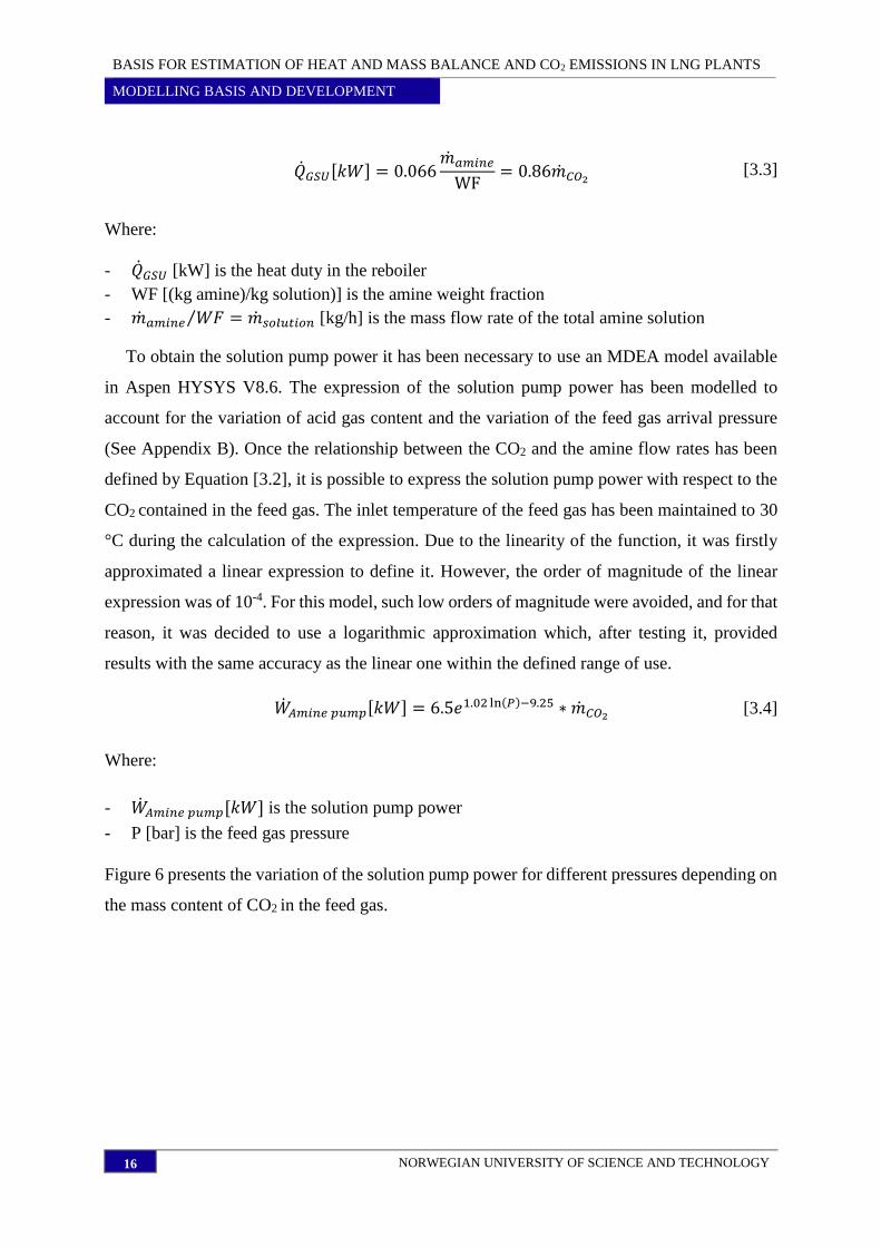
To obtain the solution pump power it has been necessary to use an MDEA model available

in Aspen HYSYS V8.6. The expression of the solution pump power has been modelled to

account for the variation of acid gas content and the variation of the feed gas arrival pressure

(See Appendix B). Once the relationship between the CO2 and the amine flow rates has been

defined by Equation [3.2], it is possible to express the solution pump power with respect to the

CO2 contained in the feed gas. The inlet temperature of the feed gas has been maintained to 30

°C during the calculation of the expression. Due to the linearity of the function, it was firstly

approximated a linear expression to define it. However, the order of magnitude of the linear

expression was of 10-4. For this model, such low orders of magnitude were avoided, and for that

reason, it was decided to use a logarithmic approximation which, after testing it, provided

results with the same accuracy as the linear one within the defined range of use.

��𝐴𝑚𝑖𝑛𝑒 𝑝𝑢𝑚𝑝[𝑘𝑊] = 6.5𝑒1.02 ln(𝑃)−9.25 ∗ ��𝐶𝑂2 [3.4]

Where:

- ��𝐴𝑚𝑖𝑛𝑒 𝑝𝑢𝑚𝑝[𝑘𝑊] is the solution pump power

- P [bar] is the feed gas pressure

Figure 6 presents the variation of the solution pump power for different pressures depending on

the mass content of CO2 in the feed gas.




Figure 6. Solution pump power for different pressures as a function of the total CO2 mass flow rate.

It was acknowledged that the feed gas inlet temperature affects the power. However, it has

been necessary to neglect its contribution for simplification. Its relative effect to the power

consumption is minor when compared to the pressure effect. The specific power by ton of CO2

absorbed as a function of the pressure and temperature has been presented in Figure 7 for a CO2

4 mol%. Both the temperature and pressure are presented within the possible operational range

of this unit. The range of temperature has been set according to the limitations of the amine, as

a minimum temperature of 30 °C is necessary for the reaction, but temperatures higher than 50

°C can lead to thermal degradation of the amine.

Figure 7. Specific pumping power variation depending on the feed gas pressure and temperature for a

CO2 content in the feed gas of 4 mol %.




The addition of a preheater was studied to account for the temperature effect, but due to

unknown temperature after the condensate stabilizer, and the low relative effect it had within

the entire model, it was decided to not add it so the complexity level was not increased.

Gas Dehydration Unit

The dehydration model has one product: dry gas that is sent to the NGL extraction. The water

removed is taken away from the process. The dehydration contribution to the energy balance

consists on the heat needed for the regeneration process of the molecular sieves.

After the CO2 is absorbed, the gas is washed with water to remove the amine traces. Due to

this, the sweetened gas is saturated with water that has to be removed by adsorption in molecular

sieves. These sieves must be regenerated by heat addition.

Different approaches were considered. Firstly, a model was simulated in HYSYS basing the

process on a simple splitter. For a defined split ratio, the simulation calculated the heat duty

needed to carry out the separation. The results obtained from the model were compared to

reference data [2] and there was a relative error of +66% with respect to the reference heat duty,

what invalidated the model in HYSYS. Alternatively, it was decided to use an analysis of the

adsorption process performed by PetroSkills [6] in order to obtain an expression for the heat

duty as a function of the gas flow rate.

The water content in the gas is highly affected by the temperature, pressure and flow rate of

the gas, and consequently different correction factors have been considered for each one of the

parameters. The reference state has been set to 30 °C and 50 bar, and the factors have been

expressed as the variation in heat duty with respect to the reference conditions. Further

explanation of the simplifications and definition of the expressions can be found in Appendix

C.

An expression has been obtained from [6] to approximate the heat duty depending on the gas

flow rate. Equation [3.5] represents this heat duty variation at reference conditions, where ��𝑔𝑎𝑠

[ton/h] represents the total flow rate of the gas at the dehydration model inlet.

��𝐷𝑒ℎ𝑦𝑑𝑟𝑎𝑡𝑖𝑜𝑛,𝑟𝑒𝑓[𝑀𝑊] = (0.03��𝑔𝑎𝑠 − 0.7) [3.5]




Figure 8 represents this variation of the heat duty depending on the gas mass flow rate. It has

been assumed valid for flow rates larger than the range defined for the definition of the

expression.

Figure 8. Dehydration heat duty as a function of the total gas mass flow rate.

The pressure to be provided in the model is the arrival pressure, and for the temperature,

because it has not been assessed an evaluation of the gas temperature after the GSU, it has been

decided to use the minimum process temperature achieved after cooling the gas stream.

The pressure correction factor has been defined by Equation [3.6], where the pressure is

defined in absolute bar.

𝐹𝑃 = −0.007𝑃 + 1.37 [3.6]

The temperature correction factor has been defined by Equation [3.7] where the temperature

is defined in °C.

𝐹𝑇 = 0.06𝑇 − 0.76 [3.7]

Figure 9 presents the percent variation of the heat duty defined by the two correction factors

defined before.




Figure 9. Graph representing the effect of the pressure and temperature on the heat duty. Each line

represents the percentage variation of the head consumption depending on each parameter.

Once the factors have been obtained, it is possible to find the regeneration heat duty for the

dehydration process from Equation [3.8]. The accuracy of this expression is limited to a lowest

process temperature of 15 °C. Below this value, the model does not provide reasonable values

of the heat duty.

��𝐷𝑒ℎ𝑦𝑑𝑟𝑎𝑡𝑖𝑜𝑛[𝑀𝑊] = (0.03��𝑔𝑎𝑠 − 0.7) ∗ 𝐹𝑃 ∗ 𝐹𝑇 [3.8]

3.4.4 NGL Extraction

This subsystem model provides two different products: gas that is sent to the liquefaction

unit, and LPG as final product. This model only accounts for upstream extraction, and it

accounts for heat duty necessary to separate the ethane from the LPG, assuming the methane

has been previously separated in a scrub column.

To model this unit, it has been necessary to define whether there is LPG production or not

in order to calculate the LNG mass flow rate consequently. Besides, it has been necessary to

define the richness level of the LNG product such that is possible to delimit its C3 and C4 content

in case LPG is also produced.

The composition options have been divided in three ranges depending on the methane content

in order to address the LNG richness: lean, medium or rich gas. Table 7 presents the defined

ranges for each composition classification depending on the methane mol%.




Table 7. Definition of the composition range of the liquefied gas components depending on the

methane mol%.

Composition C1 Minimum [mol%] C1 Maximum [mol%]

Lean 93.6 100

Medium 87.6 93.5

Rich 85| 87.5

Figure 10 presents the flow diagram of the algorithm modelled to calculate the mass balance

in the unit. Firstly, it is necessary to know whether LPG is produced or not. After this option is

defined, the richness level of the LNG product is set. In case there is LPG production and it is

also desired to obtain a medium or rich LNG product, the richness level defines the split ratio

between the LPG and the LNG product. If there is not LPG production, the richness level is

taken into account in Section 3.4.5 due to its effect on the power needs to drive the compressors

in the liquefaction process.

Figure 10. Flow diagram for the mass balance calculation in the NGL extraction unit.

In case LPG is produced, the lean classification assumes that the gas entering the liquefaction

only contain C1, C2 and nitrogen. The reason of not taking into account the C3+ is to differentiate

better between the lean and de medium classification. For the medium and rich cases, the C3

mass fraction is based on the total C3 content in the feed gas, whereas the C4 mol% is calculated

based on the gas composition at the inlet of the NGL extraction unit. Once the composition of

the gas sent to liquefaction is defined, the excess of C3 and C4 is produced as LPG.




Table 8 indicates how the LPG entering the liquefaction model is distributed for the medium

and rich classifications. The split ratio was based on the reference data [2], where only one case

had LPG production.

Table 8. Definition of the gas entering the liquefaction unit for each richness classification. These split

ratios are only applied when LPG is produced.

Component Medium Rich

C3 50% mass content in feed gas 100% mass content in feed gas

C4 1 mol% 2 mol%

A HYSYS simulation was modelled to obtain the heat duty of the de-ethanizer reboiler. A

column with a reboiler and a condenser was used for this task. Due to the operational

performance of the column, it was necessary to set the pressures inside the column as well as

the feed gas inlet parameters. Besides, the different specifications were evaluated. Two different

specifications were used for the model definition: overhead C2 mol fraction of 94 %, and C2/C3

bottom ratio of 0.02.

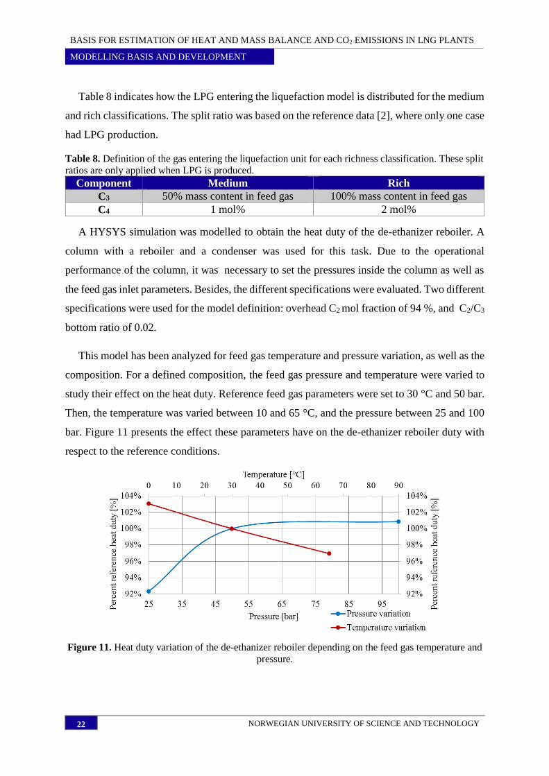
This model has been analyzed for feed gas temperature and pressure variation, as well as the

composition. For a defined composition, the feed gas pressure and temperature were varied to

study their effect on the heat duty. Reference feed gas parameters were set to 30 °C and 50 bar.

Then, the temperature was varied between 10 and 65 °C, and the pressure between 25 and 100

bar. Figure 11 presents the effect these parameters have on the de-ethanizer reboiler duty with

respect to the reference conditions.

Figure 11. Heat duty variation of the de-ethanizer reboiler depending on the feed gas temperature and

pressure.




After this analysis, it was decided to neglect the effect these parameters had because it would

have meant an increase in the complexity of the expression. Instead, it was decided to account

for the composition variation, due to its larger effect.

The composition effect has been studied under different simplifications due to the difficulties

of defining a general expression for all kinds of compositions. It has been assumed that all the

methane has been previously removed. Therefore, the gas flow rate contains all the C2, C3 and

C4. Figure 12 represents the specific reboiler duty per kg of gas entering the de-ethanizer for

different compositions. C2 has been increased from 40 to 70 mol%, and for each C2 mol fraction

the C3 has been varied. The remaining part of the gas is considered C4.

Figure 12. Specific heat duty of the de-ethanizer reboiler depending on the composition.

As it is observed from the figure above, the LPG composition affects the heat duty. For this

reason, it has been necessary to obtain an expression of the heat duty as a function of the mol

fraction of C2 and C3. To simplify, the composition is based on the NGL Extraction Unit inlet

composition, assuming all the C1 and N2 are removed upstream the de-ethanizer. It is assumed

that all the C2+ enters the de-ethanizer, and then it is later fractionated and/or reinjected to the

main gas stream that enters the liquefaction unit.

It has been assumed that the entire amount of C2 is always liquefied and produced as LNG,

regardless the definition of the LNG product richness. This simplification has been done to

avoid further complications with the split ratio in the NGL Extraction model.

The necessity of accounting for both components has increased the complexity level of the

model, but it had to be done to estimate this unit in order to get more information about the heat




needs of the LNG plant and reduce the final scaling factor that infers large uncertainties. This

variation of the composition has been approximated by the exponential expression [3.9] (see

Appendix D).

��𝑑𝑒−𝑒𝑡ℎ𝑎𝑛𝑖𝑧𝑒𝑟[𝑀𝑊] = ��𝑑𝑒−𝑒𝑡ℎ𝑎𝑛𝑖𝑧𝑒𝑟(−0.11[𝐶2] + 0.14)𝑒(20.6[𝐶2]−14.3[𝐶2]+5.4)∗[𝐶3] [3.9]

Where:

- ��𝑑𝑒−𝑒𝑡ℎ𝑎𝑛𝑖𝑧𝑒𝑟 [kg/h] refers to the total C2+ at the inlet of the NGL extraction unit

- [𝐶2] is the mol fraction of ethane

- [𝐶3] the mol fraction of propane

Equation [3.9] has to be used within the composition range analyzed. Very low ethane

content relative to the propane mol% leads to a high specific power per kg of mass flow rate,

and for these situations, the de-ethanizer should be modelled differently to correctly estimate

its duty.

3.4.5 Liquefaction unit

This unit is based on exergy calculations, and its only product is LNG at 1.1 bar. Therefore,

the calculations do not only account for the liquefier, but the End flash to fulfill the

specifications. However, the End flash gas calculations are further assessed in Section 3.4.6.

The power consumption of this unit is all addressed to the compressor power requirement of

the liquefaction unit.

As stated in previous sections, the model accounts for four different liquefaction process

types: Advanced Mixed Refrigerant (AMR), which includes Dual Mixed Refrigerant (DMR)

and Mixed Fluid Cascade (MFC), Propane Pre-cooled Mixed Refrigerant (C3MR), Single

Mixed Refrigerant (SMR) and N2 expander process. Besides, three different correction factors

have been obtained to address the feed gas temperature, pressure and feed composition effect

on the power needs.

In first instance, HYSYS models were considered for each one of the process types. To

correctly model these processes, it was necessary to optimize the refrigerant composition

depending on the feed gas composition. The optimization of the mixed refrigerant composition

implied a thorough procedure that resulted to be unreasonably complex for the present model.




Therefore, this option was rejected, and it was decided to use an exergy analysis that implied

simple calculations and easiness to account for the different aspects of the process, obtaining a

flexible expression valid for its implementation in Microsoft Excel.

The exergy difference between inlet and outlet of the process is used to estimate the total

available work between the two states. This difference is calculated through the enthalpy and

entropy of each state using Equation [3.10]. For that, the outlet state has been used as reference

state, fixing the pressure of 1.1 bar and the bubble point temperature of the LNG (-161.7 °C for

the reference pressure and composition). The inlet state has been varied to include the effect of

the variation in temperature and pressure of the gas entering the unit in the model. The heat

rejection temperature of the process (see Section 3.4.1) has been used to define the feed gas

inlet temperature, whereas the pressure, affecting the enthalpy and entropy, has been set to the

arrival pressure.

Δ𝑒1−2[𝑘𝐽

𝑘𝑔] = (h − 𝑇0s)𝐿𝑁𝐺 − (h − 𝑇0s)𝑓𝑒𝑒𝑑 [3.10]

Where:

- 𝑒 [kJ/kg] is the specific exergy

- h [kJ/kg] is the specific enthalpy

- 𝑇0 [°C] is the heat rejection temperature of the process

- s [kJ/kg] is the specific entropy

Once the total reversible work is calculated, it is necessary to account for the specific

efficiency of the liquefaction process type, in order to estimate the power need of each specific

process type.

Efficiency calculation

The reference efficiency calculation has been based on reference specific power

requirements for the different process types [2]. Equation [3.11] defines the calculation of the

exergy efficiency, which compares the total reversible work during the liquefaction against the

real power requirements of the process itself. These efficiencies are consistent with the use of

the mass flow rate at the liquefaction inlet.




𝜂𝑒𝑥𝑒𝑟𝑔𝑦[−] =Δ𝑒1−2

𝑤𝑟𝑒𝑎𝑙 [3.11]

Where 𝑤𝑟𝑒𝑎𝑙 [kJ/kg] is the real work obtained from the reference data and Δ𝑒1−2 [kJ/kg] is the

exergy difference at reference inlet and outlet state for the lean gas composition.

The exergy difference used for the efficiency calculation has been the obtained for the lean

gas case stated in Table 10 because the reference data is referred to a lean gas. These efficiencies

have been kept constant at all times, assuming they are not affected by the parameters

considered in the correction factors. Table 9 presents the three different efficiencies that have

been obtained for the characterization of the model. AMR and C3MR processes are assumed to

have the same efficiency due to minor differences. The relative efficiency of these processes

has been validated against additional reference data [7].

Table 9. Exergy efficiencies of the different process types.

Process type Exergy efficiency [-] Relative AMR/C3MR

AMR, C3MR 0.45 100

SMR 0.41 91

N2 0.32 71

Correction factors

Three different factors have been necessary to reflect the inlet process temperature, feed

pressure and composition variations. These factors are modelled to reflect the percent variation

in reversible specific work with respect to the reference inlet state mentioned above.

Two independent correction factors have been obtained for the temperature and pressure

correction. A correction factor for the composition effect was obtained following the same

principle as the temperature and pressure factors to reflect the exergy difference variation as a

result of the composition variation. For simplification, the temperature and the pressure factors

are assumed to be valid regardless the gas composition variation, whereas the composition

correction factor has been assumed to be valid for every temperature and pressure within the

stated range.

The pressure correction factor has been obtained for a pressure range between 25 and 100

bar. This factor has been defined by Equation [3.12] where the pressure is expressed in absolute

bar.




𝐾𝑃[% 𝑟𝑒𝑓𝑒𝑟𝑒𝑛𝑐𝑒] = −0.27 ln(𝑃) + 2.06 [3.12]

The pressure effect has been tried with a polynomial and a logarithmic expression in order

to choose the most accurate approximation. After the analysis, the logarithmic expression was

chosen due to its better definition of the process energy needs within the defined range of study.

The temperature correction factor has been obtained for a temperature range between 0 and

65 °C. This factor has been expressed by Equation [3.13] where the temperature is expressed in

°C.

𝐾𝑇[% 𝑟𝑒𝑓𝑒𝑟𝑒𝑛𝑐𝑒] = −0.01𝑇 + 0.74 [3.13]

For 𝐾𝑇, a linear and a polynomial expression where tried. In this case, the linear expression

better fit the temperature variation.

Further information about the approximations of 𝐾𝑃 and 𝐾𝑇 can be found in Appendix E.

The composition correction factor has been obtained for three different compositions, which

have been classified depending on the methane content. Table 10 presents the reference

compositions representing the three possible classifications of the gas richness.

Table 10. Reference compositions and KC definition depending on the gas richness

Component Lean Medium Rich

Methane 0.974 0.92 0.87

Ethane 0.0124 0.068 0.062

Propane 0.0045 0.003 0.04

Butane 0.0019 0.002 0.021

Pentane 0.00 0.00 0.00

Nitrogen 0.0072 0.007 0.007

KC 1.05 1 0.89

The data curves and points represented by the obtained correction factors are shown in Figure

13.




Figure 13. Graph representing the effect of the pressure, temperature and composition on the work

consumption. Each line represents the percentage variation of the work consumption depending on

each parameter.

Model expression

After obtaining the efficiencies and the correction factors, Equation [3.14] has been obtained

to calculate the power needs of the liquefaction drivers. This equation, as for the efficiency

expression, is consistent with the mass flow rate at the liquefaction unit inlet.

��𝐿𝑖𝑞[𝑘𝑊] =��𝐿𝑖𝑞 ∗ ∆𝑒𝑟𝑒𝑓𝑒𝑟𝑒𝑛𝑐𝑒 ∗ 𝐾𝑃 ∗ 𝐾𝑇 ∗ 𝐾𝐶

𝜂𝑒𝑥𝑒𝑟𝑔𝑦 [3.14]

Where:

- ��𝐿𝑖𝑞 [kW] is the power consumption of the liquefaction drivers

- ��𝐿𝑖𝑞[kg/h] is the gas flow rate at the inlet of the liquefaction unit model

- 𝜂𝑒𝑥𝑒𝑟𝑔𝑦 is the exergy efficiency of the chosen process type

- ∆𝑒𝑟𝑒𝑓𝑒𝑟𝑒𝑛𝑐𝑒 = 497 [kJ/kg] is the reference reversible work at 50 bar and 30 °C for medium

gas richness

Based on Equation [3.14], the specific power for the process types available in the model, at

reference conditions, is presented in Table 11.

Table 11. Specific power based on the reference conditions, for a medium gas richness.

Process type Specific power [kWh/ton LNG]

AMR/C3MR 307

SMR 337

N2 expander 431




3.4.6 End flash

For this model, it has been assumed that the flash gas is used for fuel gas. It may be the case

that the fuel gas needs are higher than the End flash flow rate, in which case fuel gas should be

taken for instance from the BOG or regasifying LNG. This would complicate the GHV

calculation due to the different gas compositions, and to simplify, it has been assumed that the

End flash gas is sufficient to cover the gas turbine needs.

The End flash model has been defined to allow a maximum of 1 mol% nitrogen in the final

LNG product. Figure 14 presents the flow diagram followed to calculate the nitrogen split ratio.

The End flash split ratio is based on the N2 content in the gas after the liquefaction model. If

the N2 content is lower than 1 mol%, all the N2 is assumed to be contained in the final LNG

product. If the N2 content is higher, 1 mol% of the N2 is maintained in the final LNG product,

whereas the excess N2 is assumed to be removed by the End flash. As the fuel is supposed to

be taken from the End flash, it is assumed that there is gas flashed even though an End flash is

not necessary because the LNG product fulfills the N2 mol% specification after the liquefaction

unit.

Figure 14. Flow diagram for the N2 Mass balance calculation.

A simulation with HYSYS was performed to obtain the composition of the flash gas and

enable the calculation of the GHV for the fuel gas. During the simulation, it was assumed that

the liquefied gas after the expansion was at 1.1 bar and bubble point temperature for the

reference composition. This gas entered a flash to separate the vapor and liquid phase. The C1

was varied from 85 to 98 mol% for different nitrogen mol fractions in order to analyze the effect

it had in the flash gas composition. The remaining liquid was approximated to ethane, as it was

acknowledged that there was no variation between choosing C2, C3 or C4 because it all remained




at liquid phase. Figure 15 presents the C1 mass fraction in the flash gas depending on the C1 and

nitrogen content of the liquefied gas at the inlet of the End flash model.

Figure 15. Flash gas mass percentage relative to the total gas flow rate, as a function of the C1 and N2

in the liquefied gas.

It can be observed that the higher the C1 content in the liquefied gas is, the higher the

concentration of C1 in the gas flashed. The effect of the nitrogen mol% variation in the inlet gas

has been also analyzed. It can be seen in Figure 15 that both curves, representing different

nitrogen contents in the liquefied gas entering the End flash, provide a similar methane mass

fraction in the flash gas. Thus, it has been assumed that the N2 content variation in the liquefied

gas entering the End flash model is negligible.

Assuming that the flash gas only contains C1 and nitrogen, it is possible to obtain the GHV

of the flash gas, and thus the fuel gas needs. Equation [3.15] defines the content of C1 in the

flash gas as a function of the C1 mol% in the gas entering the model based on the curves

presented in Figure 15. The function has been approximated to a polynomial expression because

a linear approximation implied deviations that could easily be avoided by the polynomial one.

𝐶1,𝑓𝑙𝑎𝑠ℎ [%𝑤𝑡] = 1.9(𝐶1,𝑙𝑖𝑞𝑢𝑒𝑓𝑖𝑒𝑑)2 − 2.2𝐶1,𝑙𝑖𝑞𝑢𝑒𝑓𝑖𝑒𝑑 + 1.2 [3.15]

Where 𝐶1,𝑓𝑙𝑎𝑠ℎ is the mass fraction in the flash gas and 𝐶1,𝑙𝑖𝑞𝑢𝑒𝑓𝑖𝑒𝑑 the mol fraction in the gas

at the inlet of the model.

The GHV has been calculated on a mass basis to enable the calculation of the fuel gas flow

rate through Equation [3.16].




𝐺𝐻𝑉𝑔𝑎𝑠 [𝑘𝐽

𝑘𝑔] = ∑ 𝑤𝑖 ∗ 𝐺𝐻𝑉𝑖

𝑁

𝑖=1

[3.16]

Where:

- 𝑤𝑖 [% kg] the mass fraction of the component i

- 𝐺𝐻𝑉𝑖 [kJ/kg] is the ideal mass calorific value of the component i at 25 °C [8]

Further discussion of the fuel gas calculation can be found in Section 3.4.9.

3.4.7 Total power and heat duty calculations

Total power consumption

To account for the total electrical consumption of the systems that were not modelled, the

work obtained from adding power needs for the liquefaction unit and the amine solution pump

in the GSU has been increased by 30%. This scaling was obtained after analyzing different

reference cases [2] and evaluating the model accuracy for different percentages. A list of the

main systems that are included within this parameter are listed below:

- Compression systems: Condensate, off-gas, LPG, BOG, Flash/fuel gas

- Pumping systems: Cooling system, LNG loading, booster pumps, hot oil, reflux pumps, air

compressors, and FLNG thrusters.

- Administration office facilities

Equation [3.17] defines the total power consumption in the LNG plant, which includes both the

power needs of the liquefaction unit and the electrical power of the plant.

��𝑡𝑜𝑡𝑎𝑙 = 1.3(��𝐿𝑖𝑞 + ��𝐴𝑚𝑖𝑛𝑒 𝑝𝑢𝑚𝑝) [3.17]

Heat consumption

To account for the heat needs of the systems that were not modelled, the heat duty obtained

from the addition of the GSU and dehydration unit heat duties has been increased by 20%. This

scaling was obtained after analyzing the information available from the reference cases [2]. A

list of the main systems that are included within this parameter are presented below:




- Preheaters: Air intake of the gas turbines, GRU unit

- Condensate stabilization

- NGL fractionation: de-propanizer, de-butanizer

- Fuel gas heater

Equation [3.18] defines the total heat duty of the LNG plant.

��𝑇𝑜𝑡𝑎𝑙 = 1.2(��𝐺𝑆𝑈 + ��𝐷𝑒ℎ𝑦𝑑𝑟𝑎𝑡𝑖𝑜𝑛 + ��𝑑𝑒−𝑒𝑡ℎ𝑎𝑛𝑖𝑧𝑒𝑟) [3.18]

3.4.8 Drivers

Three different drivers are considered for this model: LM6000 representing aeroderivative

turbines, Frame 7 representing the heavy-duty turbines and electrical motors powered by the

electrical grid. For the turbine models, the thermal efficiency of each type has been defined and

corrected depending on the ambient air temperature. For the electrical motors, a CO2 emissions

factor has been defined for different power systems.

Efficiency calculation of gas turbines

The efficiency of the gas turbine will only reflect the effect of the ambient air temperature

variation. Therefore, it will not account for other possible losses due to ageing, fouling…etc.

Then, the expression for the modified efficiency as a function of the ambient air temperature is:

𝜂𝐺𝑇 = 𝜂𝐺𝑇,𝑑𝑒𝑠𝑖𝑔𝑛 ∗ 𝑓(𝑇) [3.19]

Where 𝜂𝐺𝑇,𝑑𝑒𝑠𝑖𝑔𝑛 is the efficiency of the turbine at design point. 𝑓(𝑇) is a function of the air

ambient temperature which has to be introduced in °C.

The temperature variance of the model has been constrained to temperatures above 0 °C. In

case the temperature is lower, the model assumes the same efficiency as for 0 °C. Besides, 𝑓(𝑇)

has been assumed linear for both turbine models.

LM6000

The LM6000 has been characterized with a 𝜂𝐺𝑇,𝑑𝑒𝑠𝑖𝑔𝑛 of 38%. Figure 16 presents the

efficiency variation of the LM6000 as a function of the ambient air temperature.




Figure 16. LM6000 efficiency at different ambient temperature (adapted from [9]).

This function has been approximated by Equation [3.20] in order to implement this variation

on the spreadsheet model.

𝑓(𝑇) = (−1.3𝑇 + 121)/100 [3.20]

Frame 7

The Frame 7 has been characterized with a 𝜂𝐺𝑇,𝑑𝑒𝑠𝑖𝑔𝑛 of 28%. Figure 17 presents the

efficiency variation of the Frame 7 as a function of the ambient air temperature.

Figure 17. Frame 7 efficiency at different ambient temperature (adapted from [10]).

As for the LM6000, the function defining the efficiency has been approximated to Equation

[3.21].

𝑓(𝑇) = (−0.59T + 109.4)/100 [3.21]




Electrical grid

The larger availability of the electrical grid, as well as the emissions reduction, has increased

the interest of providing new LNG plant projects with power from it.

The electrical grid has been defined to partly or fully cover the needs of the plant. Depending

on the desired ratio between the gas turbines and the electrical grid usage, the fuel gas

calculation and the CO2 emissions are calculated consequently. The electrical grid is assumed

to only cover the electrical needs of the plant, whereas the heating needs are covered by the

combustion of fuel gas. In case gas turbines and the grid are used simultaneously, the waste

heat from the gas turbines is assumed sufficient to cover the heating needs.

The CO2 emission estimations are obtained based on the configuration of the plant. A CO2

emissions estimation based on the fuel gas combustion can be found in Section 4.3.5, whereas

a CO2 emissions factor to account for the electrical power consumption from the grid has been

described below.

Two different options have been addressed in the model: electricity imported from a local

station, and electricity from the region electrical grid.

For the local station case, it has been necessary to obtain an estimation of the CO2 depending

on the type of power generation plant that provides the electricity. For this task, three different

types of power plants have been defined: combined cycle plant, coal fired plant and renewable

energy plant. Typical CO2 emissions have been obtained from reference data [11, 12]. The CO2

estimation is assumed to be an approximation because the values obtained can vary largely

depending on individual conditions of each plant and the local climate. Table 12 presents the

CO2 emissions per electrical MJ consumed in the LNG plant.

Table 12. Definition of the efficiencies for each one of the power plants types, and scaling factor for

estimation of the CO2 emissions for each one.

Plant Type CO2 emissions [kg/MWh]

Combined cycle 360

Coal fired 740

Renewable 0

For the case in which the electricity is taken from the regional grid, no assessment has been

performed because of the large range of possibilities. Therefore, the emissions factor for this

option must be provided as an input in order to estimate the emissions.




3.4.9 Fuel gas calculation

A fuel gas model has been necessary to account for the gas taken to produce the required

power. The model calculates the amount of fuel gas necessary for the total power production,

as well as the final LNG production after the End flash gas removal.

One of the main issues during the model design was the decision of where the fuel gas would

be taken from. Figure 18 shows a typical fuel gas balance in an LNG plant. It is usual to get the

End flash gas, the BOG from tanks and the ship vapor return in order to supply the gas turbines

with fuel. However, sometimes the flash gas may not be sufficient, or it may not be valid as a

fuel gas due to its high nitrogen content that might make it unsuitable for the gas turbines.

Besides, the BOG and ship vapor return, fixed by design, often are not sufficient by themselves

to cover the fuel needs. An alternative option is to take the gas after the slug catcher, but this

option is not as widely used as for the other cases, being commonly used only for startup of the

plant.

Figure 18. Typical fuel gas balance in LNG plants (source: BP).

Due to the spreadsheet limitations, it was too complex to implement a model that obtained

the fuel gas from all the different possibilities. It has been decided to use the End flash intake

due to its more extended use and availability than the other options (see Appendix F for

upstream fuel gas intake alternative). BOG and ship vapor return were considered to contribute

to some extent to the End flash gas intake, but it was finally discarded due to the complexities

it entailed.




The model then assumes that fuel gas is only taken from the End flash. Once the End flash

gas composition is obtained through Equation [3.15], and thus the GHV of this gas calculated,

it is possible to estimate the fuel gas flow rate that is necessary to run the gas turbines through

Equation [3.22].

��𝑓𝑢𝑒𝑙[𝑡𝑜𝑛

ℎ] =

��𝐺𝑇

𝐺𝐻𝑉 ∗ 𝜂𝐺𝑇 [3.22]

Where:

- ��𝑓𝑢𝑒𝑙 [kg/s] is the fuel gas consumption

- ��𝐺𝑇 [MJ/kg] involves all the power needs of the LNG plant covered by the gas turbines.

- 𝐺𝐻𝑉 [MJ/kg] is the e Gross Heating Value of the End flash gas

- 𝜂𝐺𝑇 [-] is the efficiency of the gas turbine

In case the electrical grid is used, Equation [3.22] must be specified for the total heat duty

instead of the power needs.

Once the fuel gas flow rate has been calculated, it is possible to estimate the amount of CO2

emitted due to the combustion of this fuel gas. As the End flash is assumed to only contain

methane and nitrogen, and the latter does not contribute to the emissions, a very simple reaction

has been defined in Equation [3.23] to obtain the CO2 from the combustion.

𝐶𝐻4 +1

2𝑂2 → 𝐶𝑂2 + 2𝐻2 [3.23]

The mol flow rate of methane in the fuel gas is obtained from the fuel mass flow rate, and

then the amount of CO2 produced can be obtained through the reaction defined above.


MODEL TESTING


4 MODEL TESTING

The model has been tested against six different real cases [2]. All these cases provide

information about the liquefaction power, the LNG, LPG and Condensate production, and the

CO2 emissions from the feed and from the total power consumption and heat generation.

Besides, two different cases provide further information about the electrical power and heating

needs of different units, the fuel gas consumption and the total power consumption and heat

duty.

A comparison of the production rates, liquefaction power needs and CO2 emissions has been

performed and compared for all the cases. Besides, the remaining estimations have been

compared against the available data.

The results have been expressed as the relative error of the estimation with respect to the

reference data. The numerical data of all the comparisons is summarized in Appendix G.

4.1 Reference cases

Benchmarking data

The reference data [2] for benchmarking is presented in the present section. Table 13

presents the plant parameters, Table 14 the feed gas and process parameters and Table 15 and

feed gas composition. Besides, Table 16 and Table 17 provide the different data that has been

compared to the model estimations.

Table 13. Main Plant parameters of the benchmarking cases.

Plant parameters Case A Case B Case C Case D Case E Case F

Type of plant FLNG Onshore Onshore FLNG FLNG FLNG

Compressor

drivers Aero GT Aero GT

Industrial

GT Aero GT Aero GT Aero Gt

Cooling method Water Water Air Water Air Air

Nominal capacity 3.3 4.3 13.5 3.1 4.4 4

Process type AMR AMR C3MR AMR SMR N2

expander

The flow rate in case C is originally given in Sm3 per year. To perform the calculations it

was necessary to provide a flow rate in mass basis, and to do that the density has been calculated

for standard conditions, and the flow rate has been calculated for a yearly production of 350

days, consistent with the number of production days later used for onshore LNG plants.


MODEL TESTING


Table 14. Main feed gas and process parameters of the benchmarking cases.

Feed gas and process

parameters

Case A Case B Case C Case D Case E Case F

Flow rate [ton/h] 615 816 1800 474 638 533

Arrival pressure 67 70 70 67 55 70

Mean cooling water

temperature °C 14 7.0 - 12.0 - -

Mean air temperature, °C 27.3 7.0 23.0 28.0 30.0 27.0

Table 15. Feed gas composition in mol percent of the benchmarking cases.

Feed gas

composition, % mol

Case A Case B Case C Case D Case E Case F

Methane 79.8 80.5 97.7 96.5 95.1 94.3

Ethane 4.3 5.1 1.3 1.2 2.8 0.6

Propane 1.5 2.6 0.3 0.4 0.3 3.4

n-Butane 0.3 0.8 0.1 0.1 0.1 0.1

i-Butane 0.4 0.5 0.1 9,1 0.0 0.1

n-Pentane 0.2 0.5 0.0 0.0 0.0 0.3

i-Pentane 0.2 0.5 0.0 0.0 0.0 0.2

C6+ 3.0 1.8 0.1 1.0 0.2 0.1

Nitrogen 0.9 2.5 0.2 0.7 0.2 0.1

Carbon dioxide 9.4 5.2 0.2 0.0 1.3 0.8

Table 15 presents the reference data that has been compared against the model estimations.

For the production of each product, it has been necessary to assume a number of operation days.

For the FLNG plants the operation days was set to 330 days, whereas for the onshore plants it

was set to 350. Only one of the six cases produces LPG, and it has not been possible to validate

the model for this product.

Table 16. Reference values for liquefaction power, mass balance and CO2 emissions.

Parameter Case A Case B Case C Case D Case E Case F

Liquefaction

power, MW 125.0 162.0 660.0 124.0 196.0 225.0

LNG production,

Mtpa 3.3 4.2 13.5 3.1 4.1 3.6

LPG production,

Mtpa 0 0.3 0.0 0.0 0.0 0.0

Condensate

production, Mtpa 0.3 0.7 0.3 0.05 0.01 0.2

CO2 from feed, tpa 995,000 640,000 120,000 23,000 150,000 83,000

CO2 from power

and heat

generation, tpa

797,000 900,000 3,7000,000 820,000 1,355,000 990,000


MODEL TESTING


Table 17 presents the additional reference data that was compared to the model estimations.

Each model provided information about different parameters, and these values were used to

analyze the accuracy of the model.

Table 17. Reference values for work and heat balance for cases A and B.

Parameter Case A Case B

Work balance

Total power consumption, MW 180 218

MDEA pump power, MW 5.1 3.3

Fuel gas, ton/h 42 40

Heat balance

Total heat duty, MW 138 147

MDEA solution regenerator heat duty, MW 96 63

Gas dehydration Unit heat duty, MW 3.8 8.9

De-ethanizer heat duty, MW 15.45 7.5

4.2 Testing results for the six cases

The results have been split depending on the estimated parameter. Afterwards, All the cases

have been grouped and analyzed to study the overall model performance. Table 18 contains the

model results for the six cases. These are the estimations that have been compared to the

reference data stated in Table 16.

Table 18. Model results used for benchmarking of the six cases.

Benchmarking

results Case A Case B Case C Case D Case E Case F

Liquefaction power,

MW 117.4 156.2 585.7 128.6 250.0 241.7

LNG, Mtpa 3.0 4.6 13.1 3.2 4.2 3.4

LPG, Mtpa 0 0.25 0 0 0 0

Condensate, Mtpa 0.62 0.72 0.08 0.19 0.05 0.11

CO2 from feed, tpa 898,588 725,906 80,454 0 169190 83738

CO2 from liq.

drivers, power/heat

generation, tpa

690,563 732399 4,245,612 732422 1,473,602 1,358,925

4.2.1 Liquefaction power

Figure 19 shows the discrepancy between the liquefaction power of the reference data and

the obtained model estimations.


MODEL TESTING


Figure 19. Relative error percentage in liquefaction power for the six cases.

The model has demonstrated a correct estimation of the liquefaction power. Case E presents

the largest relative error of +28% with respect to the reference data, which is well above the

rest of the cases, presenting deviations lower than +/-10%.

The possible source of error for case E was analyzed. This case is the only one using Single

Mixed Refrigerant process type. The liquefaction power was recalculated using the AMR

efficiency instead, to see if the efficiency set for the SMR process type was wrong. For the

AMR efficiency, the relative error decreased to +21%. This estimation is still above all the

remaining cases, and therefore this analysis concludes that the efficiency definition of the SMR

process type is not the source of error of this case, ignoring then the reason why this liquefaction

power error is that large.

4.2.2 LNG production

Figure 20 shows the discrepancy between the reference LNG production data and the model

estimations.


MODEL TESTING


Figure 20. Relative error percentage in LNG production for the six cases.

The LNG production has been accurately approximated for the six cases. All of them have

presented a relative error lower than +/-11%.

4.2.3 LPG production

Figure 21 presents the discrepancy between the reference LPG production data and the

model estimations. This estimation only accounts for case B because the LPG production data

was zero in the rest of the reference cases.

Figure 21. Relative error in the LPG production for case B.

For the only case analyzed, the LPG production estimation presents a relative error -16%.

This result correctly approximates the production rate of the reference data, but more reference

cases should be compared in order to validate the model. The different split ratios modelled to

reflect the LNG richness in the extraction unit model have to be improved.


MODEL TESTING


4.2.4 Condensate production

Figure 22 presents the discrepancy between reference Condensate production data and the

model estimations.

Figure 22. Relative error percentage in the Condensate production for the six cases.

For this estimation, only case B provides a valid result of the Condensate production. The

model was defined to produce all the C5+ content as Condensate, and this simplification did not

correctly estimate the total Condensate production. An overestimation of the Condensate

production can be explained by the simplification stated above, but it has not been found a

reason why there is an underestimation for cases C and F. The molecular weight simplification

for the C6+ can lead to high deviations in case the real mean molecular weight differs largely

from the C6, and the increase of the accuracy during the calculation of the mean molecular

weight might decrease the deviation in the underestimation cases, but this possible decrease

does not justify the deviation of both cases.

4.2.5 CO2 emissions from feed gas

Figure 23 presents the relative error of the estimation of CO2 emissions due to its removal in

the GSU unit. Case D has not been compared because the provided composition does not

present any CO2 content.


MODEL TESTING


Figure 23. Relative error percentage in the CO2 emissions from feed for the six cases.

The model has presented a close agreement with the assumption made. Due to the strict

requirements in the LNG, it was assumed that all the CO2 in the feed gas was removed. The

estimation in case C presents a relative error of -33%, but for this case the mass flow rate was

also approximated for an assumption of 350 production days per year. If the production days

are assumed to be 330 days instead, the flow rate per hour increases from 1800 ton/h to 1909

ton/h, and the relative error of this CO2 emissions estimation decreases to -29%. Therefore, the

estimation for case C has been accepted as valid.

4.2.6 CO2 emission from liquefaction drivers, electrical power and heat generation

Figure 24 presents the estimation of the CO2 produced due to the liquefaction drivers,

electrical power and heat generation.

Figure 24. Relative error percentage in the CO2 emissions from the liquefaction drivers, electrical

power and heat generation for the six cases.


MODEL TESTING


The simplified model has shown to be an accurate estimation for the CO2 emissions, with a

relative error range between -19% and +37%. Case F appears to be the only one exceeding the

limit of +/-30%, and it has been analyzed to find the source of this deviation.

Cases A and F have been compared using the available data to analyze the validity of the

reference data CO2 emissions for case F. Both cases are FLNG plants and use aeroderivative

turbines, and their total power consumption are available for comparison. In case A, the kg of

CO2 emitted per MWh generated is 576 kg/MWh, whereas for case F is 432 kg/MWh. This

implies a relative difference of -25% with respect to the emissions of case A. The CO2 emissions

for case F using 576 kg/MWh results in 1,244,205 tpa, what implies a relative deviation of the

model estimation of -9%, a result much closer than the reference data provided for case F. This

analysis concludes that the real CO2 emissions from the power and heat generation in case F

could be higher than the value provided.

4.2.7 Validation of the cases

Figure 24 presents the results grouped by case to analyze the validity of the model. The

Condensate production estimations have been discarded. Disregarding the unrepresentative

results discussed above, the model has provided estimations with deviations well below the

maximum tolerated of +/- 30% for all the cases.

Figure 25. Results summary for the six different cases.

The model has demonstrated to provide valid estimations for the liquefaction power, the

LNG production, and the CO2 emissions. Cases A and D present the most accurate results with


MODEL TESTING


a relative error within +/-13% in all the estimations presented. The CO2 estimation from the

feed in case C has to be further studied, as it is the only estimated parameter within the four

representative parameters for this case that presents an unusual deviation with respect to the

reference data.

4.3 Testing results for cases A and B

Cases A and B have been additionally tested for the total power and heat duty consumption,

MDEA solution pump power, dehydration duty, de-ethanizer reboiler duty and fuel gas flow

rate. Table 19 presents the additional model results for the six cases. These estimations have

been only compared to the available data from cases A and B, whereas the others have been

commented in case unusual estimations were obtained.

Table 19. Additional model results for the six cases.

Benchmarking

results Case A Case B Case C Case D Case E Case F

Total power, MW 159.3 208.4 762 167.2 326.0 314.9

Total heat duty, MW 143.7 132.6 109.1 12.6 68.8 208.4

MDEA solution

regenerator, MW 98.3 74.9 8.3 0 18.5 9.2

MDEA solution

pump, MW 5.2 4.1 0.46 0 0.8 0.5

De-ethanizer, MW 13.7 31.2 11.1 3.7 3.8 140.8

Dehydration, MW 7.8 4.4 71.15 6.8 35.0 23.6

Fuel gas flow rate,

ton/h 46.8 49.2 220.2 41.2 84.5 85.2

Fuel gas GHV

[kJ/kg] 37700 35580 46434 45400 44512 40745

4.3.1 Total power and heat duty

Figure 26 presents the relative error percentage of the total power and heat duty with respect

to the reference data.


MODEL TESTING


Figure 26. Relative error percentage in the Total electrical power and heat duty.

The total power and heat duty present a deviation between -12% and +4%. The scaling

factors used for these estimations were defined after analyzing the two cases, showing a close

agreement for both of them.

Besides, the results of all the remaining cases have been analyzed, and it has been observed

that low CO2 content in the gas leads to a very low CO2 regenerator duty, and as the total heat

duty is scaled from it, this low values lead to very low total heat duty that should be revised.

4.3.2 MDEA solution pump and regenerator

Figure 27 represents the relative error percentage of the GSU model, that entails the MDEA

solution regenerator heat duty and pump power.

Figure 27. Relative error percentage in the MDEA solution regenerator and pump power model.


MODEL TESTING


The CO2 regenerator and solution pumps have shown to accurately estimate their respective

values. Case A presents a negligible deviation for both, whereas case B has presented larger

deviations, always below the maximum deviation accepted.

According to the Total heat duty estimation for the rest of the cases, the MDEA solution

regenerator and pump model provides very low heat duties. These results have to be compared

in order to analyze whether the model is valid for low CO2 content feed gas or not.

4.3.3 Dehydration

Figure 28 shows the relative error percentage of the dehydration model with respect to the

reference data.

Figure 28. Relative error percentage in the dehydration heat duty model

The dehydration unit has presented relevant deviations. Case A presents a deviation of

+104% relative to the real data, whereas case B relative deviation is -50%. The reference

analysis [6] was only based on two different pressures and temperatures, and this thesis work

assumed the dependence of the heat duty with respect to these parameters to be linear.

Therefore, it is necessary a more detailed dehydration model, possibly based on the reference

procedure, to define correctly the correction factors that account for the temperature and

pressure.

4.3.4 De-ethanizer

Figure 29 represents the relative error percentage of the de-ethanizer unit with respect to the

reference data. The de-ethanizer model has presented disparities for the two cases. Case A


MODEL TESTING


provides an estimation with a deviation of -12%. On the other hand, case B presents a deviation

of +316%, invalidating this model estimation.

Figure 29. Relative error percentage in the de-ethanizer heat duty model.

The model has been analyzed for these two cases. The estimated duty for case A is 13.66

MW and 30.19 MW for the case B. It has been found that the difference derives from the total

mass flow rate, and therefore the mass balance definition. The specific heat duty in kWh per kg

of gas was similar for both cases, but due to the split ratios defined in the model, as well as the

assumption that considers that all the C2+ flows through the de-ethanizer, case B accounted for

a much higher gas flow rate.

It has been observed that the total heat duty for case F appears to be quite high. The specific

heat duty in kWh per kg has shown to be 0.26 kWh/kg, what represents twelve times the specific

heat duty for cases A and B. This high value has been addressed to the low ratio C2/C3 that

appears to be out of the model range.

4.3.5 Fuel gas flow rate

Figure 30 shows the relative error percentage in the model of the fuel gas flow rate with

respect to the reference data.


MODEL TESTING


Figure 30. Relative error percentage in the fuel gas flow rate model.

The fuel gas flow rate model has provided estimations for both cases which are larger than

the real data ones. Case A presents a relative error of +11%, whereas case B presents a +25%.

These results validate the simplified model used for the fuel gas calculation


CONCLUSION


5 CONCLUSIONS AND RECOMMENDATIONS

The model has demonstrated to provide accurate estimations through the implementation of

simple expressions that correctly defined the processes. The results present a deviation well

below the limit established for the LNG production, the liquefaction power and the CO2

estimations. These estimations have been provided for a wide range of variants, what implies

that the model defined presents a reliable tool for calculation of these parameters. Moreover,

the LPG production, the Gas Sweetening Unit, the fuel gas flow rate and the scaling factors

defined for the total power and heat duty have been correctly estimated. These models have

presented as well deviations below the set limits of +/-30%. However, the range has been

limited to the available data, and larger deviations could be expected in case the plant evaluated

differs from the validated cases.

A summary of the conclusions deduced from the model test are presented:

- Correct estimations have been provided for the liquefaction power, LNG, and CO2

emissions

- Condensate estimations present deviations over +/- 100%due to the mass balance

simplifications in the Separation model.

- LPG production has provided a deviation of -16% that validates the model for the only case

compared

- The scaling factor for the total power and heat duty estimations have been validated,

providing results with relative error between -12 and + 4%.

- The Gas Sweetening Unit model has correctly defined the MDEA regenerator heat duty and

pumping power for CO2 feed gas content over 5 mol%.

- The dehydration model has to be redefined to correctly calculate the heat duty of this unit.

- The de-ethanizer model assumption regarding the mass flow rate entering the unit has

invalidated the model

- The intake of the fuel gas from the End flash has presented accurate results that validate the

model simplifications.


CONCLUSION


Additionally, the following recommendations are suggested based on the conclusions

reached:

- A split ratio should be defined to estimate the Condensate production

- The Gas Sweetening Unit should be validated for low CO2 content feed gas

- A dehydration model, possibly based on the procedure followed in [6] should be created

for a better definition of the process

- The LPG split ratio can be further developed to account for more detailed LNG richness

definition and LPG production rate. Moreover, more cases with LPG production should be

studied to validate the model over a wider range of plant configurations

- The assumptions in the mass flow entering the de-ethanizer model should be redefined,

accounting for a more realistic mass flow rate instead of the entire C2+ content in the feed

gas.

- The mass balance implemented in the End flash model can be further developed to provide

a better definition of the LNG product composition. This upgrade would lead to an

estimation of the GHV of the LNG, improving the basis for the project assessment and

economic analysis.

- The fuel gas model should be defined to allow simultaneously different intake options. The

fuel gas composition has to be defined in detail in order to obtain more accurate estimations


REFERENCES


6 REFERENCES

[1] S. Mokhatab, J. Mak, J. V. Valappil, and D. A. Wood, Handbook of liquefied natural

gas, First edition. ed. Amsterdam: Elsevier, GPP, 2014.

[2] J. Petterssen, Senior Specialist, Statoil. Personal Communication, email.

[3] Y. Bramoullé, "LNG quality and market flexibility challenges and solutions," Total Gas

& Power- Technology Division.

[4] K. Arnold and M. Stewart, Surface production operations, 2nd ed. Houston, Tex.: Gulf

Pub. Co., 1998.

[5] Gas Processors Association. and Gas Processors Suppliers Association (U.S.),

Engineering data book, 12th ed. Tulsa, Okla. (6526 E. 60th St., Tulsa 74145): Gas

Processors Suppliers Association, 2004.

[6] P. Campbell, "What is the Impact of Feed Gas Conditions on the Adsorption

Dehydration System?."

[7] J. D. Bukowski, "Natural Gas Liquefaction Technology for Floating LNG Facilities,"

ed: Air Products and Chemicals , Inc.

[8] Y. A. Cengel and M. A. Boles, Thermodynamics : an engineering approach, Seventh

edition. ed. New York, NY: McGraw-Hill, 2011.

[9] G. Energy, "LM6000 -50/60 HZ Gas Turbine Generator Set- Product Specification," ed,

2015.

[10] F. J. Brooks, "GE Gas Turbine Performance Characteristics," GE Power Systems.

[11] O. Bolland, Thermal power generation: Norges Teknisk-Naturvitenskapelige

Universitet, 2014.

[12] I. E. Agency, "Power Generation from Coal," Coal Industry Advisory BoardOctober

2010 2010.


APPENDICES


APPENDIX A: CONDENSATE STABILIZATION MODEL

Appendix A presents the defined model for the estimation of the Condensate stabilization

heat duty, that was discarded after the large deviations it presented. For the model, it was

assumed that the temperature and pressure did not affect the heating needs of the Stabilization

Unit, as it further complicate the model.

Due to the possible range compositions in the feed gas, it was not found a general model that

represented the heat duty of all the different possibilities. The heat duty in the stabilization does

not only depend on the condensate amount but on its specific composition. It was intended to

simplify the composition of the HHC into a single “mean component” and use it to obtain the

heat duty needs of the stabilization. It was then made an analysis of the different condensate

components´ phase behavior, in order to choose one component that could be representative of

the condensate composition. This component had to be removed in liquid state at typical

operational parameters of the column, that were decided to be 200 °C and 10 bar. Figure 31

presents the Pressure-Temperature curves of the different components. At this point, C6 had to

be discarded as a representative “mean component” because it did not fulfill the specifications.

Figure 31. Pressure-Temperature diagram of different pure components in the feed gas.

Afterwards, a simple model of the stabilization column was simulated in HYSYS to obtain a

heat duty estimation. The model was simulated for a reference case [2], and the condensate

composition was approximated to different mean components to study the effect this

assumption implied on the heat duty. Figure 32 presents the deviation that each mean

component simulation has with respect to the reference case data.


APPENDICES


Figure 32. Variation of the heat duty for different mean components. The graph shows the relative

variation with respect to the C8 that was decided to be used as mean component.

It was found that the model did not correctly approximated the heating needs of the unit for

any of the “mean components”. All of the calculated heat duties differ from the reference value

largely. Moreover, the relative error with respect to the reference data varies between +230 and

+292% depending on the “mean component” selection. These two facts invalidated the

assumptions and simplifications made, and alternatively it was decided to use the scaling factor

stated in Section 3.4.7 to account for the heating needs of the condensate stabilization.


APPENDICES


APPENDIX B: GAS SWEETENING UNIT CALCULATIONS

To obtain the pumping power necessary to pump the solution, a model has been developed

to obtain the power as a function of the amine mass flow rate and the pressure of the feed gas.

The process simulation tool HYSYS has been used for this purpose. An available Amine

process for acid gas removal has been used to obtain an expression of the power consumption

of the solution pump.

The process has been simulated for a CO2 content between 2 mol% and 20 mol%, and

pressures between 25 and 70 bar, for a constant feed gas inlet temperature of 30 °C. Figure 33

presents the pumping power as a function of the amine mass flow rate.

Figure 33. Pumping power consumption as a function of the Amine mass flow rate and the feed gas

inlet pressure.

All the functions have shown to be linear, and therefore defined by the expression:

�� = 𝑎 ∗ ��𝑎𝑚𝑖𝑛𝑒 + 𝑏 [B.1]

The expression for the power consumption has been found to have the form

�� = 𝑎(𝑃) ∗ ��𝑎𝑚𝑖𝑛𝑒 + 𝑏(𝑃) [B.2]

Where 𝑏(𝑃) has not been taken into account due to its negligible contribution to the function.

The function 𝑎(𝑃) has been approximated to an expression in order to represent the pressure

effect on the pumping power consumption. A linear and a logarithmic expressions were tried


APPENDICES


to study the accuracy of the final expression, being the logarithmic one more accurate for

defining the pressure effect due to the numerous decimals contained in the linear expression.

Figure 34. Parameter “a” as a function of feed gas arrival pressure.

Finally, the model function has been defined as follows:

��𝐴𝑚𝑖𝑛𝑒 𝑝𝑢𝑚𝑝[𝑘𝑊] = 𝑒1.02 ln(𝑃)−9.25 ∗ ��𝑎𝑚𝑖𝑛𝑒 [B.3]

In order to provide a better representation of the pumping power variation, the information

provided in Section 3.4.3 has been expressed as a function of the CO2 in the feed gas instead of

the amine flow rate. Besides, this power need has been tested for values of the pressure up to

100 bar with successful results, enabling the model to work under this pressure level.


APPENDICES


APPENDIX C: DEHYDRATION UNIT CALCULATIONS

The calculation of the heat duty in the dehydration process has been subjected to different

simplifications that were necessary due to its complexity when it comes to obtain all the

different parameters of the process. The different factors has been obtained under the conditions

stated in [6]. Figure 35 presents the heat duty variation depending on the gas flow rate,

temperature and pressure. These results from the reference case have been used to characterize

the expressions used in the dehydration model of this report.

Figure 35. Variation of the heating load with the feed gas rate, temperature and pressure.

The different expressions stated in Section 4.3.3 have been calculated for reference

conditions of 30 °C and 50 bar. Due to the lack of data and the limitations, several

simplifications has been done to obtain the factor:

- The correction factors have been obtained by varying the parameter of interest, while

keeping the other at its reference value.

- The heat duty expression due to the feed gas flow rate variation has been obtained at

reference conditions.

- The data only takes into account two temperatures and two pressures, therefore the factors´

behavior has been assumed linear.

- It can be appreciated from Figure 35 that, with respect to the reference conditions, the heat

duty rise at different temperatures and pressures is larger as the gas feed rate increases. This

means that the calculated factors are also dependent on the feed gas rate. However, to

consider it would have meant an excessive level of complexity that was aimed to avoid.


APPENDICES


Therefore, the effect of the gas feed rate on the temperature and pressure correction factors

was neglected.


APPENDICES


APPENDIX D: NGL EXTRACTION AND FRACTIONATION

To obtain the de-ethanizer heat duty, a model has been developed to obtain the heat duty as

a function of the gas composition. Assuming only C2+ enters the unit, the heat duty for different

compositions has been obtained by using HYSYS.

Equation [D.1] has been defined from the different curves obtained and exposed in Figure

11. The different curves have been approximated to an exponential equation as follows:

��𝑑𝑒−𝑒𝑡ℎ𝑎𝑛𝑖𝑧𝑒𝑟 [𝑘𝑊ℎ

𝑘𝑔] = 𝛼 ∗ 𝑒𝛽∗[𝐶3] [D.1]

Where ��𝑑𝑒−𝑒𝑡ℎ𝑎𝑛𝑖𝑧𝑒𝑟 [𝑘𝑊ℎ/𝑘𝑔] is the specific heat duty of the reboiler per kg of C2+ entering

the de-ethanizer and [𝐶3] is the mol fraction of propane.

Afterwards, 𝛼 and 𝛽 have been obtained as a function as a function of the mol fraction of 𝐶2.

Figure 36 presents the variation of 𝛼, that has been approximated to a linear function.

Figure 36. Parameter 𝛼 as a function of the 𝐶2 mol %.

This approximation to a linear function was a simplification, as it can be seen that the

function is not linear, but it was accepted because it did not imply a large deviation in the heat

duty estimation.

𝛼 = −0.11[𝐶2] + 0.14 [D.2]


APPENDICES


Figure 37 represents the variation parameter 𝛽, that has been approximated to a polynomial

function. In this case it was not possible to approximate it to a linear function due to the large

deviation it implied.

Figure 37. Parameter 𝛽 as a function of the 𝐶2 content.

Equation [D.3] defines the polynomial approximation that was used to describe the function

obtained.

𝛽 = 20.6[𝐶2]2 − 14.3[𝐶2] + 5.4 [D.3]


APPENDICES


APPENDIX E: LIQUEFACTION CORRECTION FACTORS

This Appendix presents the different approximations performed for the pressure and

temperature correction factors used in the model of the liquefaction unit. The Coefficient of

determination R2 was used to choose the data curve approximation.

Figure 38 presents the two approximations analyzed for 𝐾𝑃. The R2 for the polynomial

approximation was 0.9982 against 1 for the logarithmic one. Moreover, the logarithmic was

preferred due to the simplicity of the expression compared to the polynomial one.

Figure 38. Data curve approximations for the definition of 𝐾𝑃.

Figure 39 shows the two approximations analyzed for 𝐾𝑇. The R2 for the polynomial

approximations was 0.9997 against the 0.9995 for the linear one. In this case it was decided to

use the linear approximation because its accuracy was very high, and the expression was

simpler that the polynomial one.


APPENDICES


Figure 39. Data Curve approximations for the definition of 𝐾𝑇.


APPENDICES


APPENDIX F: UPSTREAM FUEL GAS INTAKE

This Appendix provides a calculation method that can be implemented on the spreadsheet

model in case the upstream fuel gas intake is preferred.

The upstream fuel gas intake assumes that all the fuel gas is taken after the slug catcher. The

power consumed by the different processes is a function of the feed gas flow rate. As the fuel

gas is directly taken from the feed gas stream, an increase in the power consumption leads to a

higher fuel flow rate, and consequently a decrease of the feed gas processed and LNG produced.

This fact makes necessary an iterative process for which the Microsoft Excel solver can been

used, as well as the formulation of some assumptions.

The composition of the fuel gas is assumed the same as the feed gas stream after the slug

catcher, and its GHV is calculated consequently. The fuel gas consumption is assumed to be

entirely spent to run the compressors, and the heating needs are assumed to be fully covered by

waste heat. Therefore, the heat generation is assumed to be fully covered by the waste heat

produced by the gas turbines.

Figure 40. Iterative algorithm used to calculate the fuel gas need.

The algorithm gives an estimation of the gas fraction left after the fuel gas removal and

obtains the total power consumption through Equation [3.17]. Then, the energy of combustion

of the fuel gas obtained is calculated through Equation [3.22] and compared to the previously


APPENDICES


calculated total power consumption. The iteration ends once the energy of combustion equals

the energy consumption of the entire plant model.

For the implementation of the upstream fuel gas intake model it is necessary to assume that

the End flash gas, the BOG and the vapor return from ship are recovered and reliquefied, so the

LNG production does not decrease.


APPENDICES


APPENDIX G: NUMERICAL TEST RESULTS

Table 20. Numerical results for the comparison of the six cases.

Pa

ram

ete

r

Refe

rence

Est

ima

teE

rro

r %

Refe

rence

Est

ima

teE

rro

r %

Refe

rence

Est

ima

teE

rro

r %

Liq

uefa

cti

on p

ow

er,

MW

125

117.4

-6162

156.2

-4660

585.7

-3

LN

G p

roducti

on,

Mtp

a3.3

3-1

04.2

4.6

10

13.5

13.1

-3

LP

G p

roducti

on,

Mtp

a0

00

0.3

0.2

5-1

60

00

Co

ndensa

te p

roducti

on,

Mtp

a0.3

0.6

2108

0.7

0.7

23

0.3

0.0

8-7

4

CO

2 fro

m f

eed,

tpa

995,0

00

898,5

88

-10

640,0

00

725,9

06

13

120,0

00

80,4

54

-33

CO

2 fro

m liq

. dri

vers

, po

wer

and h

ea

t g

enera

tio

n,

tpa

797,0

00

690,5

63

-13

900,0

00

732,3

99

-19

37,0

00,0

00

4,2

45,6

12

15

Pa

ram

ete

r

Refe

rence

Est

ima

teE

rro

r %

Refe

rence

Est

ima

teE

rro

r %

Refe

rence

Est

ima

teE

rro

r %

Liq

uefa

cti

on p

ow

er,

MW

124

128.6

4196

250

28

225

241.7

7

LN

G p

roducti

on,

Mtp

a3.1

3.2

54.1

4.2

23.6

3.4

-7

LP

G p

roducti

on,

Mtp

a0

00

00

00

00

Co

ndensa

te p

roducti

on,

Mtp

a0.0

50.1

9276

0.0

10.0

5410

0.2

0.1

1-4

7

CO

2 fro

m f

eed,

tpa

23,0

00

0-

150,0

00

169,1

90

13

83,0

00

83,7

38

1

CO

2 fro

m liq

. dri

vers

, po

wer

and h

ea

t g

enera

tio

n,

tpa

820,0

00

732,4

22

-11

1,3

55,0

00

1,4

73,6

02

9990,0

00

1,3

58,9

25

37

Ca

se F

Ca

se A

Ca

se B

Ca

se C

Ca

se D

Ca

se E


APPENDICES


Table 21. Numerical results for comparison of cases A and B.


APPENDICES


APPENDIX H: MODEL IMPLEMENTATION

Appendix H presents the different sheets contained in the testing model implemented in

Microsoft Excel to perform the calculations. As an example, case B is shown. This testing model

implemented on Microsoft Excel has been provided together with the report to give an example

of how the created model could be implemented on a spreadsheet software.


APPENDICES


Figure 41. Inputs sheet layout.


APPENDICES


Figure 42. Gas Sweetening Unit sheet layout


APPENDICES


Figure 43. Dehydration Unit sheet layout.


APPENDICES


Figure 44. NGL Extraction model composition and presentation of the mass flow to liquefaction.


APPENDICES


Figure 45. These tables present the split ratio contributing to the mass balance of the unit, and the

energy balance in the de-ethanizer to obtain the heat duty of the NGL Extraction model.


APPENDICES


Figure 46. Liquefaction Unit model layout.


APPENDICES


Figure 47. End flash composition, GHV calculation and split ratio contributing to the mass balance of

the model.


APPENDICES


Figure 48. Driver model sheet layout and CO2 emissions estimation from the liquefaction drivers,

electrical power consumption and heat generation.


APPENDICES


Figure 49. Results sheet summary presenting all the results estimated.

Basis for estimation of heat and mass balance and CO2 ...

Documents

Transcript of Basis for estimation of heat and mass balance and CO2 ...