Basics of Wave Propagation - Arraytool · 03/05/2015 · Time Harmonic FieldsHelmholtz Wave...

Time Harmonic Fields Helmholtz Wave Equation Lossy Materials Poynting Vector Reflection Summary

Basics of Wave Propagation

S. R. [email protected]

Department of Electrical & Electronics EngineeringBITS Pilani, Hyderbad Campus

May 7, 2015

Course Outline RF & Microwave Engineering, Dept. of EEE, BITS Hyderabad

mailto:[email protected]


Outline

1 Time Harmonic Fields

2 Helmholtz Wave Equation

3 Lossy Materials

4 Poynting Vector

5 Reflection

6 Summary



Complex Notation

Any time-varying field such as~F = F (x, y, z) cos (ωt + ψ) a

can be written using of Euler’s identity as,

~F = Re[F (x, y, z) ej(ωt+ψ)

]a = Re

[F (x, y, z) ejψejωt

]a = Re

[Fsejωt

]a.



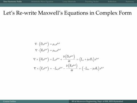
Let’s Re-write Maxwell’s Equations in Complex Form

∇ ·(~Dsejωt

)= ρe,sejωt

∇ ·(~Bsejωt

)= ρm,sejωt

∇×(~Hsejωt

)=~Je,sejωt +

∂(~Dsejωt

)∂t

=(~Je,s + jω~Ds

)ejωt

∇×(~Esejωt

)= −~Jm,sejωt −

∂(~Bsejωt

)∂t

=(−~Jm,s − jω~Bs

)ejωt



So, Maxwell’s Equations in Complex Form are ...

∇ · ~Ds = ρe,s

∇ ·~Bs = ρm,s

∇× ~Hs =~Je,s + jω~Ds

∇×~Es = −~Jm,s − jω~Bs



Outline



3 Lossy Materials

4 Poynting Vector

5 Reflection

6 Summary



Wave

The wave shown in the above diagram can be represented as

F (x, t) = sin (βx− βvt) = sin (βx−ωt) (1)

where,ω = 2πf = βv. (2)



Wave Equation

Simple 1 - dimensional wave equation is given as

∂2F∂x2 =

1v2

∂2F∂t2

Using the complex notation, the above equation can be simplified as

∂2Fs

∂x2 =

(β

ω

)2

(jω)2 Fs = −β2Fs

⇒ ∂2Fs

∂x2 + β2Fs = 0 (3)

Using the theory of linear differential equations, solution for the above equation is given as

Fs = Aejβx + Be−jβx

⇒ F = Re[(

Aejβx + Be−jβx)

ejωt]= Re

[Aej(ωt+βx) + Bej(ωt−βx)

]. (4)



Now, let’s prove that time harmonic electromagnetic fields exist inthe form of waves ...



Helmholtz Wave EquationIn a source-less dielectric medium,

∇ · ~Ds = 0

∇ ·~Bs = 0

∇× ~Hs = jω~Ds = jωε~Es (5)

∇×~Es = −jω~Bs = −jωµ~Hs (6)

Taking curl of (6) gives

∇×(∇×~Es

)= ∇×

(−jωµ~Hs

)⇒ ∇

(∇ ·~Es

)−∇2~Es = −jωµ

(∇× ~Hs

)⇒ ∇

(∇ ·~Es

)−∇2~Es = −jωµ

(jωε~Es

)⇒ ∇2~Es = ∇

(∇ ·~Es

)−ω2µε~Es

⇒ ∇2~Es =~0−ω2µε~Es (7)

Similarly, it can be proved that

∇2~Hs = −ω2µε~Hs. (8)



Finally, Let’s Analyze the Helmholtz Wave Equation

Let’s compare general wave equation (3) and Helmholtz wave equation (7).

∂2Fs∂x2 + β2Fs = 0 ∇2~Es + ω2µε~Es = 0

From the above comparison, we get,

β = ω√

µε. (9)

But, we already knew that

v =ω

β.

So, from the above equations, we get

v =1√

µε=

1√

µrεrc (10)

where c is the light velocity.



Solution of Helmholtz EquationVector Helmholtz equation can be decomposed as shown below:

∇2Exs + ω2µεExs = 0

∇2~Es + ω2µε~Es = 0 ∇2Eys + ω2µεEys = 0

∇2Eys + ω2µεEys = 0

Since all the differential equations are similar, let’s solve just one equation using variable-separablemethod. If Exs can be decomposed into

Exs = A (x)B (y)C (z)

then substituting the above equation into Helmholtz equation gives

∇2Exs + ω2µεExs = 0

⇒ ∂2Exs

∂x2 +∂2Exs

∂y2 +∂2Exs

∂z2 + ω2µεExs = 0

⇒ B (y)C (z)∂2A∂x2 + A (x)C (z)

∂2B∂y2 + A (x)B (y)

∂2C∂z2 + ω2µεA (x)B (y)C (z) = 0

⇒ 1A (x)

∂2A∂x2 +

1B (y)

∂2B∂y2 +

1C (z)

∂2C∂z2 −γ2 = 0



Solution of Helmholtz Equation ... Cont’d

⇒ 1A (x)

∂2A∂x2 +

1B (y)

∂2B∂y2 +

1C (z)

∂2C∂z2 −γ2 = 0

⇒ 1A (x)

∂2A∂x2 +

1B (y)

∂2B∂y2 +

1C (z)

∂2C∂z2 −γ2

x−γ2y−γ2

z = 0 (11)

The above equation can be decomposed into 3 separate equations:

1A (x)

∂2A∂x2 − γ2

x = 0

1B (y)

∂2B∂y2 − γ2

y = 0

1C (z)

∂2C∂z2 − γ2

z = 0

It is sufficient to solve only one of the above equations and it’s solution is given as

⇒ ∂2A∂x2 − γ2

xA (x) = 0

⇒ A (x) = L1eγxx + L2e−γxx = L−eγxx + L+e−γxx (12)



Solution of Helmholtz Equation ... Cont’d

So, finally Exs is given as

Exs =(L−eγxx + L+e−γxx) (M−eγyy + M+e−γyy) (N−eγzz + N+e−γzz) (13)

⇒ Ex = Re[(

L−eγxx + L+e−γxx) (M−eγyy + M+e−γyy) (N−eγzz + N+e−γzz) ejωt]

(14)

with the conditionγ2

x + γ2y + γ2

z = γ2. (15)



Outline



3 Lossy Materials

4 Poynting Vector

5 Reflection

6 Summary



Complex Permittivity

∇ · ~Ds = ρe,s

∇ ·~Bs = ρm,s

∇× ~Hs =~Je,s + jω~Ds = σ~Es︸︷︷︸conduction current

+ jωε~Es︸︷︷︸displacement current

= jω

ε(

1− jσ

ωε

)︸︷︷︸

εs

~Es

∇×~Es = −~Jm,s − jω~Bs

• From now onwards, we will be using complex permitivity εs = ε(1− j σ

ωε

)instead of simple

ε when ever possible.• Another important definition is that of loss tangent:

tan θ =σ

ωε



Propagation Constant

So, from the previous slide, for lossy dielectrics, εs is a complex number and is given as

εs = ε(

1− jσ

ωε

).

Then propagation constant γ is given from the equation

γ2 = −ω2µεs

= −ω2µε(

1− jσ

ωε

)= −ω2µε + jωµσ. (16)

From the above equation, γ can be written as γ = α + jβ. Now, we need to find out the values of αand β. We have

γ2 = (α + jβ)2 =(α2 − β2)+ j (2αβ) (17)

Comparing (16) and (17) we get,

α2 − β2 = −ω2µε

β =ωµσ

2α. (18)



Propagation Constant ... Contd

Solving the set of equations (18) gives

α2 −(ωµσ

2α

)2= −ω2µε

⇒ 4α4 −ω2µ2σ2 = −4α2ω2µε

⇒ 4α4 + 4α2ω2µε−ω2µ2σ2 = 0

⇒ 4ξ2 + 4ξω2µε−ω2µ2σ2 = 0

⇒ ξ =ω2µε

2

[±√

1 +( σ

ωε

)2− 1

]

⇒ α =√

ξ = ω

√√√√ µε

2

[√1 +

( σ

ωε

)2− 1

]. (19)

Similarly it can be proved that

β = ω

√√√√ µε

2

[√1 +

( σ

ωε

)2+ 1

](20)



Skin Depth

Skin Depth:The distance δ, through which the wave amplitude decreases by a factor 1

e is called skin depth orpenetration depth of the medium, that is

E0e−αδ =E0

e.

From the above equation,

δ =1α

(21)



Outline



3 Lossy Materials

4 Poynting Vector

5 Reflection

6 Summary



Poynting Vector

One Vector Identity:

∇ ·(~A×~B

)= ~B ·

(∇×~A

)−~A ·

(∇×~B

)From the above vector identity,

∇ ·(~E× ~H

)= ~H ·

(∇×~E

)−~E ·

(∇× ~H

)= ~H ·

(−~Jm −

∂~B∂t

)−~E ·

(σ~E +

∂~D∂t

)

=

(~H ·~0− ~H · ∂~B

∂t

)−(

σ~E ·~E +~E · ∂~D∂t

)

=

(−µ~H · ∂~H

∂t

)−(

σ~E ·~E + ε~E · ∂~E∂t

)

= −(

µ~H · ∂~H∂t

+ ε~E · ∂~E∂t

)− σ~E ·~E = −

µ12

∂(~H · ~H

)∂t

+ ε12

∂(~E ·~E

)∂t

− σ~E ·~E

= − ∂

∂t

(µ

2

∥∥∥~H∥∥∥2+

ε

2

∥∥∥~E∥∥∥2)− σ

∥∥∥~E∥∥∥2.



Poynting Vector ... Cont’d

⇒ ∇ ·(~E× ~H

)= − ∂

∂t

(µ

2

∥∥∥~H∥∥∥2+

ε

2

∥∥∥~E∥∥∥2)− σ

∥∥∥~E∥∥∥2

⇒˚∇ ·

(~E× ~H

)dv =

˚ (− ∂

∂t

(µ

2

∥∥∥~H∥∥∥2+

ε

2

∥∥∥~E∥∥∥2)− σ

∥∥∥~E∥∥∥2)

dv

⇒‹ (

~E× ~H)· ~dS︸︷︷︸

???

= − ∂

∂t

˚ (µ

2

∥∥∥~H∥∥∥2+

ε

2

∥∥∥~E∥∥∥2)

dv︸︷︷︸Rate of decrease of stored Energy

−˚

σ∥∥∥~E∥∥∥2

dv︸︷︷︸Ohmic power dissipated



Poynting Vector ... Physical Interpretation

~P = ~E× ~H =∥∥∥~E∥∥∥ ∥∥∥~H∥∥∥ sin θk (22)



Instantaneous & Time Average Power

Instantaneous power corresponding to the above set of voltage & current is defined as

Pinst (t) = v0i0 cos (ωt + φ1) cos (ωt + φ2)

=v0i0

2[cos (ωt + φ1 + ωt + φ2) + cos (ωt + φ1 −ωt− φ2)]

=v0i0

2[cos (2ωt + φ1 + φ2) + cos (φ1 − φ2)] (23)

Time average power is defined as

Pavg =1

T0

ˆ T0

0Pinst dt =

v0i02

cos (φ1 − φ2) (24)



Time Average Power - Complex Notation

vreal = v0 cos (ωt + φ1) vcomplex = V = v0ej(ωt+φ1)

ireal = i0 cos (ωt + φ2) icomplex = I = i0ej(ωt+φ2)

Pavg =v0 i0

2 cos (φ1 − φ2) Pavg = 12 Re (VI∗) = v0 i0

2 cos (φ1 − φ2)



Instantaneous & Time Average Poynting Vector

~Pinst = ~Einst × ~Hinst

~Pavg = Re[

12

(~Es × ~H∗s

)]



Plane Wave in Free Space ... Poynting Vector



Free Space / Uniform Dielectric Medium Impedance

In source-less medium,

∇×~Es = −jω~Bs

⇒ ∇×(E0e−γzzx

)= −jωµ~Hs

⇒ ~Hs =j

ωµ

[∇×

(E0e−γzzx

)]=

jωµ

[∇×

(E0e−γzzx

)]=

jωµ

[∂Exs

∂zy]=

jωµ

[∂ (E0e−γzz)

∂zy]

=

(−jγ0

ωµ

)Exsy =

−j(jω√

µεs)

ωµExsy

So,

Exs

Hys=

√µ

εs=

√jωµ

σ + jωε.

Wave

Pro

pag

ati

on

Dir

ect

ion

For loss-less case (i.e., α = 0 and σ = 0),

Exs

Hys=

ωµ

β=

ωµ

ω√

µε=

√µ

ε.



Outline



3 Lossy Materials

4 Poynting Vector

5 Reflection

6 Summary



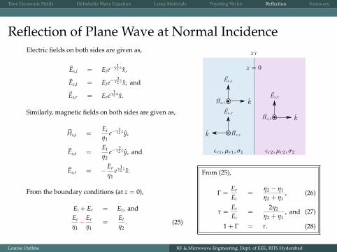
Reflection of Plane Wave at Normal IncidenceElectric fields on both sides are given as,

~Es,i = Eie−γ1z zx,

~Es,t = Ete−γ2z zx, and

~Es,r = Ereγ1z zx.

Similarly, magnetic fields on both sides are given as,

~Hs,i =Ei

η1e−γ1

z zy,

~Es,t =Et

η2e−γ2

z zy, and

~Es,r = − Er

η1eγ1

z zx.

From the boundary conditions (at z = 0),

Ei + Er = Et, andEi

η1− Er

η1=

Et

η2. (25)

x

From (25),

Γ =Er

Ei=

η2 − η1

η2 + η1, (26)

τ =Et

Ei=

2η2

η2 + η1, and (27)

1 + Γ = τ. (28)



Outline



3 Lossy Materials

4 Poynting Vector

5 Reflection

6 Summary



Summary


Basics of Wave Propagation - Arraytool · 03/05/2015 · Time Harmonic FieldsHelmholtz Wave...

Documents

Transcript of Basics of Wave Propagation - Arraytool · 03/05/2015 · Time Harmonic FieldsHelmholtz Wave...