1. APOORVA GUPTA(11972)

2. JYOTI ( 11973)

M.Sc. (Mathematical Sciences- STATISTICS)

2014-2015

Under the supervision of

Dr. Gulab Bura

Department of Mathematics and Statistics,

AIM & ACT

Basic Terminologies related to Queuing theory

Content• Stochastic process• Markov process• Markov chain• Poisson process• Birth death process• Introduction to queueing theory• History• Elements of Queuing System• A Commonly Seen Queuing Model• Application• Future plan• References

Stochastic process

Definition : A stochastic process is family of timeindexed random variable where t belongs toindex set . Formal notation , where I is anindex set that is subset of R.

Examples :

• No. of telephone calls are received at a switchboard.Suppose that is the r.v. which represents thenumber of incoming calls in an interval (0,t) ofduration t units.

• Outcomes of X(t) are called states .

}:{ ItX t tX

tX

• Discrete time , Discrete state space

• Discrete time , Continuous state space

• Continuous time , Discrete state space

• Continuous time, Continuous state space

Stochastic process is classified in four categories on the basis of state space and time space

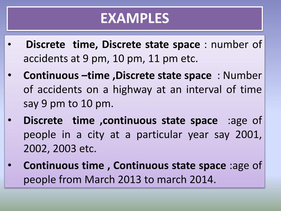
EXAMPLES

• Discrete time, Discrete state space : number ofaccidents at 9 pm, 10 pm, 11 pm etc.

• Continuous –time ,Discrete state space : Numberof accidents on a highway at an interval of timesay 9 pm to 10 pm.

• Discrete time ,continuous state space :age ofpeople in a city at a particular year say 2001,2002, 2003 etc.

• Continuous time , Continuous state space :age ofpeople from March 2013 to march 2014.

MARKOV PROCESS

If is a stochastic process such that ,given thevalues of X(t) , t >s ,do not depend on the values of X(u) ,u<s,then the process is said to be a Markov process.

• A definition of such a process is given as :

If for ,

the process is a markov process .

}),({ TttX

tttt n ...21

})(,...,)(|)(Pr{ 11 nn xtXxtXxtX

})(|)(Pr{ nn xtXxtX

}),({ TttX

)}(|)(Pr{)}(),(|)(Pr{ sXtXuXsXtX

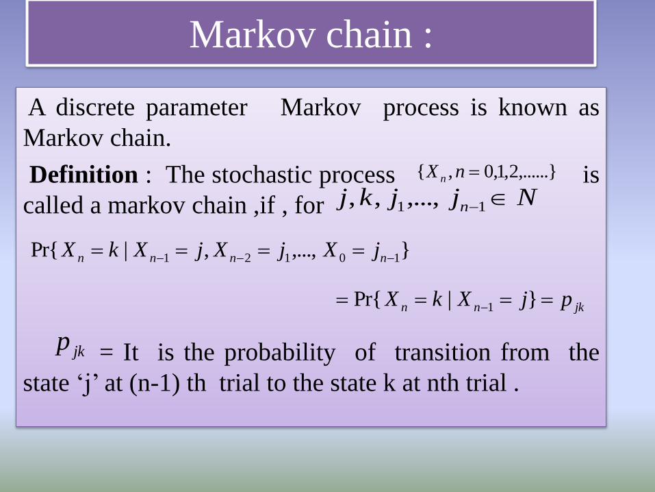
Markov chain :

A discrete parameter Markov process is known as

Markov chain.

Definition : The stochastic process is

called a markov chain ,if , for

= It is the probability of transition from the

state ‘j’ at (n-1) th trial to the state k at nth trial .

,......}2,1,0,{ nX n

Njjkj n 11,...,,,

},...,,|Pr{ 10121 nnnn jXjXjXkX

jknn pjXkX }|Pr{ 1

jkp

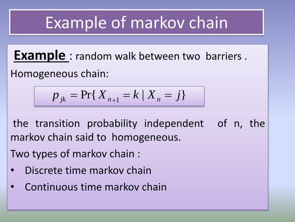
Example of markov chain

Example : random walk between two barriers .

Homogeneous chain:

the transition probability independent of n, themarkov chain said to homogeneous.

Two types of markov chain :

• Discrete time markov chain

• Continuous time markov chain

}|Pr{1

jXkXp nnjk

• A stochastic process {N(t), t>0} with discretestate space and continuous time is called apoisson process if it satisfies the followingpostulates:

1. Independence

2. Homogeneity in time

3. Regularity

The Poisson Process

10

• Independence:

N( t+h)-N(t), the number of occurrence in theinterval (t,t+h) is independent of the number ofoccurrences prior to that interval.

• Homogeneity in time:

pn(t) depends only on length ‘t’ of the interval and isindependent of where this interval is situated i.e.pn(t) gives the probability of the number ofoccurrences in the interval (t1 , t+t1 ) (which is oflength ‘t’) for every t1 .

Postulates for Poisson Process

Regularity In the interval of infinite small length

h, the probability of exactly one occurrence is

λh+o(h) and that of occurrence of more than one is

of o(h).p1 (h)= λh+o(h)

)(2

hOhpk

k

)(10 hohhP

λ= rate of arrival

Probability of zero arrival

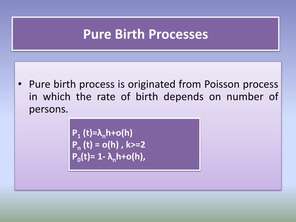
• Pure birth process is originated from Poisson processin which the rate of birth depends on number ofpersons.

Pure Birth Processes

P1 (t)=λnh+o(h) Pn (t) = o(h) , k>=2P0(t)= 1- λnh+o(h),

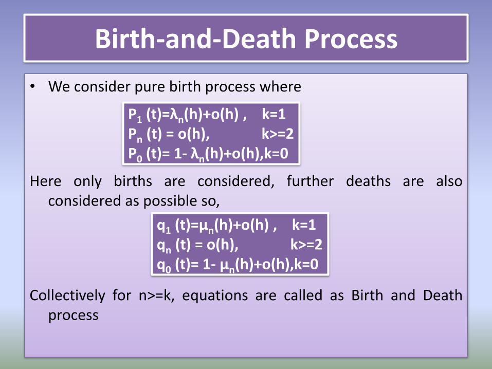
Birth-and-Death Process

• We consider pure birth process where

Here only births are considered, further deaths are alsoconsidered as possible so,

Collectively for n>=k, equations are called as Birth and Deathprocess

P1 (t)=λn(h)+o(h) , k=1Pn (t) = o(h), k>=2P0 (t)= 1- λn(h)+o(h),k=0

q1 (t)=μn(h)+o(h) , k=1qn (t) = o(h), k>=2q0 (t)= 1- μn(h)+o(h),k=0

• Note: The foundation of many of the mostcommonly used queuing models

Birth – equivalent to the arrival of a customer

Death – equivalent to the departure of a servedcustomer

15

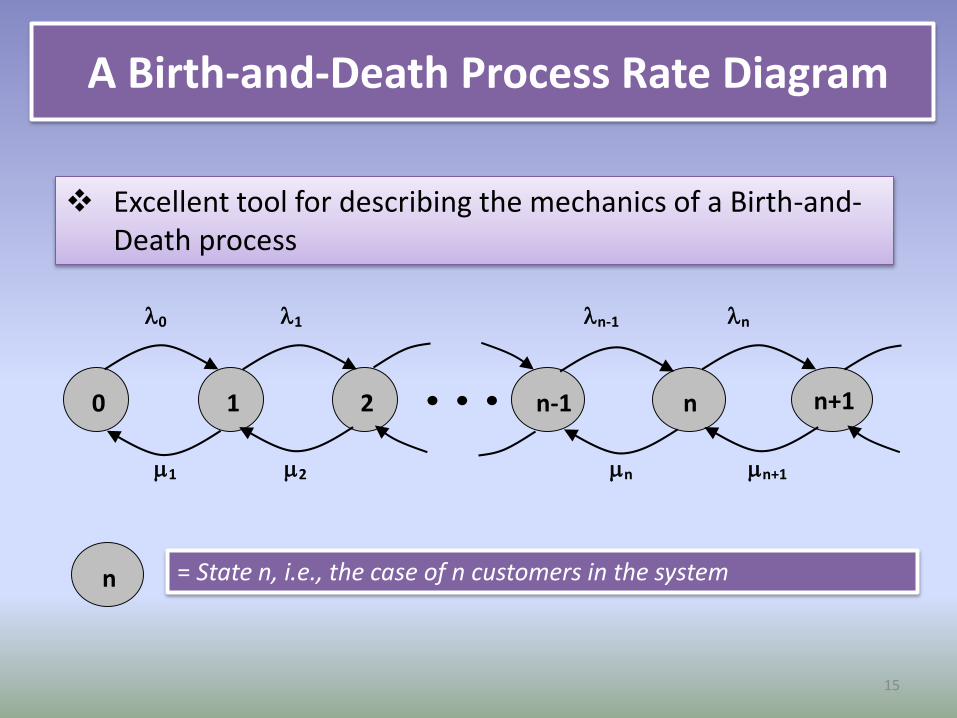
A Birth-and-Death Process Rate Diagram

0 1 n-1 n

0 1 2 n-1 n n+11 2 n n+1

n = State n, i.e., the case of n customers in the system

Excellent tool for describing the mechanics of a Birth-and-Death process

Introduction of Queueing theory

• Queueing theory is the mathematical study ofwaiting lines, or queues.

• In queueing theory a model is constructed so thatqueue lengths and waiting times can be predicted.

• Queueing theory is generally considered a branchof operations research because the results are oftenused when making business decisions about theresources needed to provide a service.

DEFINITION • A queue is said to occur when the rate at which the

demand arises exceeds the rate at which service isbeing provided.

• It is the quantitative technique which consists ofconstructing mathematical models for various typesof queuing systems.

• Mathematical models are constructed so that queuelengths and waiting times can be predicted whichhelps in balancing the cost of service and the costassociated with customers waiting for service

HISTORY• Queueing theory’s history goes back

nearly 105 years.

• It is originated by A. K. Erlang in 1909, inDanish when he is at his work place.

• Agner Krarup Erlang, a Danish engineerwho worked for the CopenhagenTelephone Exchange, published the firstpaper on what would now be calledqueueing theory in 1909.

• He modeled the number of telephonecalls arriving at an exchange by a Poissonprocess.

• Johannsen’s “Waiting Times and Number of Calls”seems to be the first paper on the subject.

• But the method used in this paper was notmathematically exact and therefore, from the pointof view of exact treatment, the paper that hashistoric importance is A. K. Erlang’s, “The Theory ofProbabilities and Telephone Conversations”

• In this paper he lays the foundation for the place of

Poisson (and hence, exponential) distribution in

queueing theory.

• His most important work, Solutions of Some

Problems in the Theory of Probabilities of

Significance in Automatic Telephone Exchanges , was

published in 1917, which contained formulas for loss

and waiting probabilities which are now known as

Erlang’s loss formula (or Erlang B-formula) and delay

formula (or Erlang C-formula), respectively.

Agner Krarup Erlang, 1878–1929

Elements of Queuing System

Service process

Queue Discipline

Number of servers

Elements of Queuing Models

Arrival process

Customer’s Behavior

System capacity

1. Arrival Process

Arrivals can be measured as the arrival rate or the interarrival

time (time between arrivals).

• These quantities may be deterministic or stochastic (given by a

probability distribution).

• Arrivals may also come in batches of multiple customers,

which is called batch or bulk arrivals.

• The batch size may be either deterministic or stochastic.

Interarrival time =1/ arrival rate

2.Customer’s Behaviour

• Balking: If a customer enters a system anddecides not to enter the queue since it is toolong is called Balking.

• Reneging: If a customer enters the queue butafter sometimes loses patience and leaves it iscalled Reneging.

• Jockeying: When there are 2 or more parallelqueues and the customers move from onequeue to another to change his position is calledJockeying.

25

3. Service Process

• Service Process determines the customer servicetimes in the system.

• As with arrival patterns, service patterns may bedeterministic or stochastic. There may also bebatched services.

• The service rate may be state-dependent. (This is theanalogue of impatience with arrivals.)

Note that there is an important difference betweenarrivals and services. Services do not occur whenthe queue is empty.

26

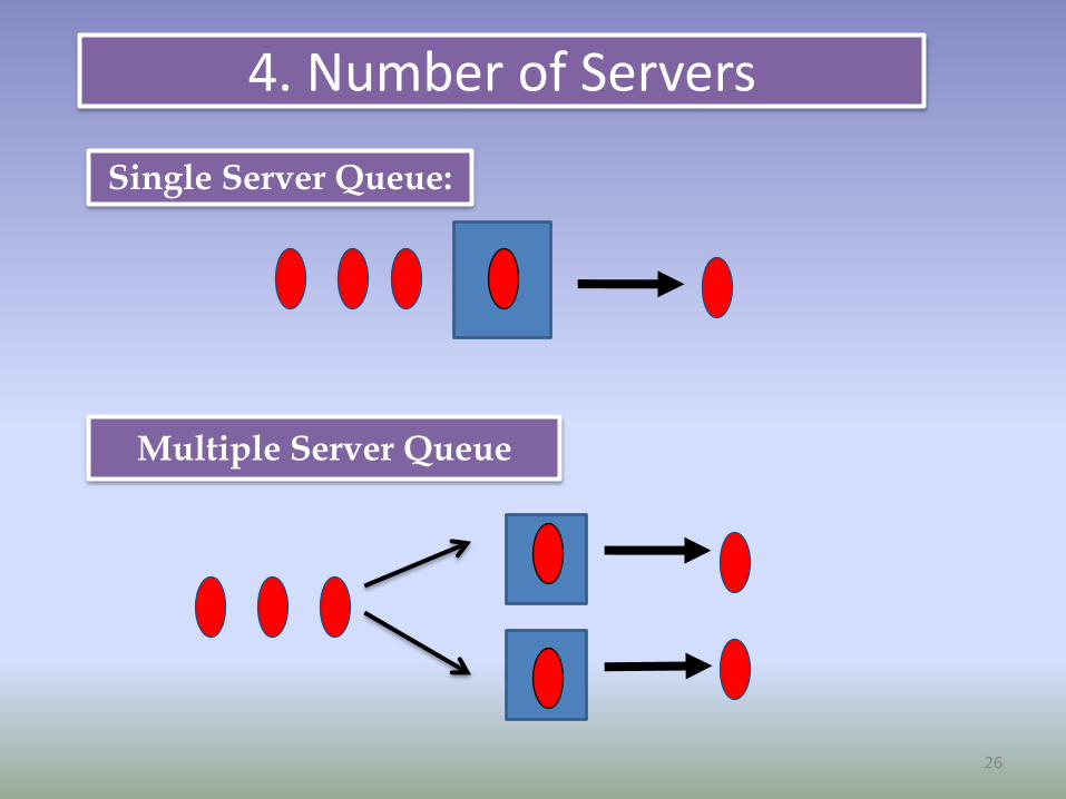
4. Number of Servers

Single Server Queue:

Multiple Server Queue

Multiple Queue with Multiple Server

Multiple Queue with Single Server

5. Queue Discipline

• FIFO- First in First out

Or FCFS- First Come First Serve

• LIFO-Last in First out

• SIRO- Service in Random order

• Priority based

FIFO- First in First out

LIFO-Last in First out

SIRO“Service In Random Order”

• Lottery system

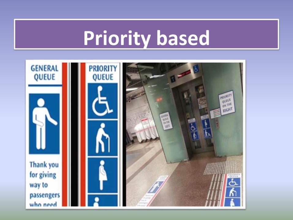
Priority based

6.System capacity

• The capacity of a system can be finite or infinite.There are many queuing systems whose capacity isfinite. In such cases problem of balking arises. It isknown as forced balking. In forced balking customerneeds the service but due to the problem of limitedcapacity of the system the customer leaves thesystem.

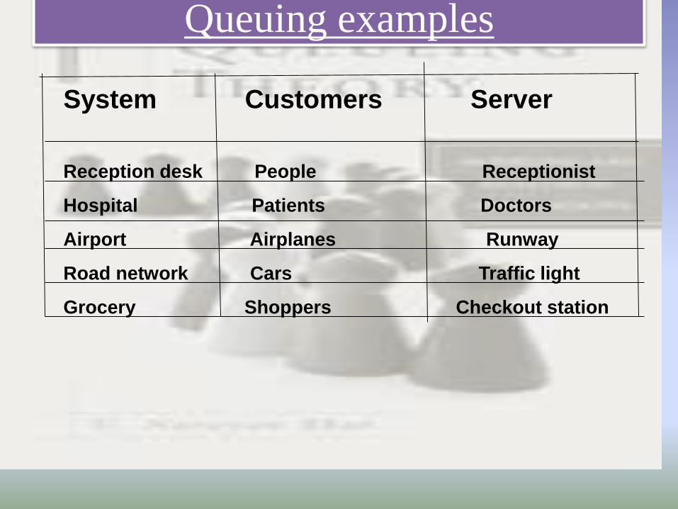
System Customers Server

Reception desk People Receptionist

Hospital Patients Doctors

Airport Airplanes Runway

Road network Cars Traffic light

Grocery Shoppers Checkout station

Queuing examples

A Commonly Seen Queuing Model• Service times as well as inter arrival times are assumed

independent and identically distributed

– If not otherwise specified

• Commonly used notation principle: A/B/C

– A = The inter arrival time distribution

– B = The service time distribution

– C = The number of parallel servers

• Commonly used distributions

– M = Markovian (exponential) - Memory less

– D = Deterministic distribution

– G = General distribution

• Example: M/M/1

– Queuing system with exponentially distributed service andinter-arrival times and 1 server

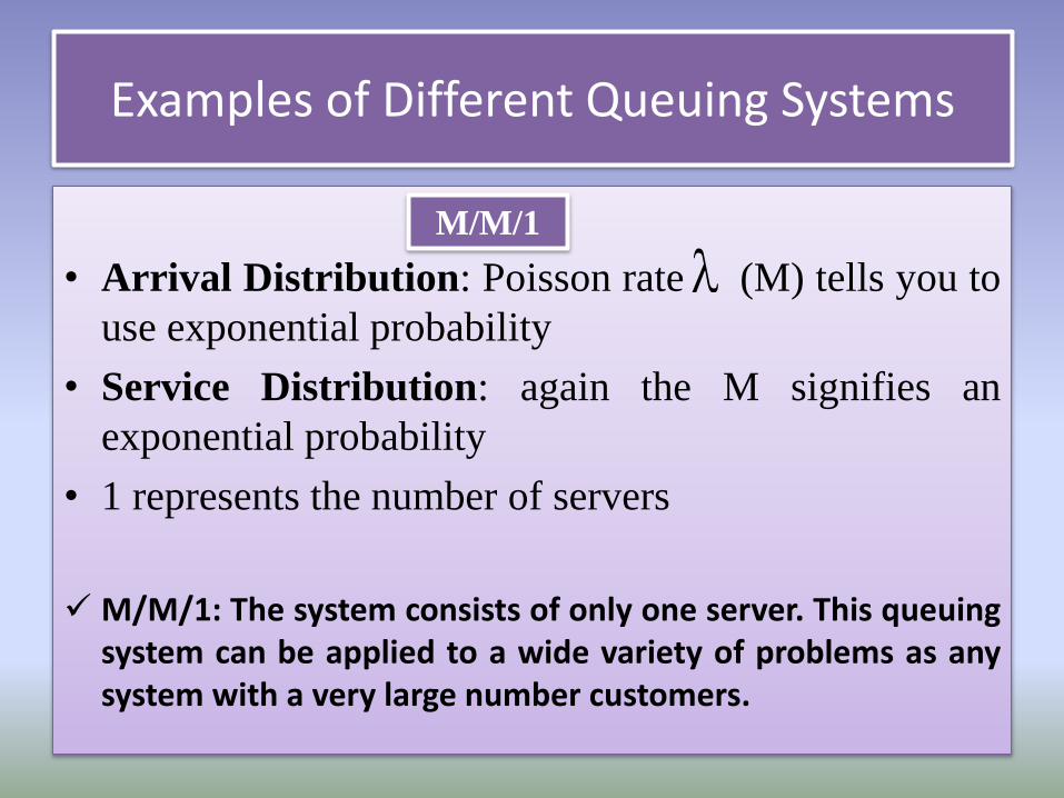
Examples of Different Queuing Systems

• Arrival Distribution: Poisson rate (M) tells you to

use exponential probability

• Service Distribution: again the M signifies an

exponential probability

• 1 represents the number of servers

M/M/1: The system consists of only one server. This queuingsystem can be applied to a wide variety of problems as anysystem with a very large number customers.

M/M/1

M/M/1 queueing systems assume a Poisson arrivalprocess.This assumption is a very good approximation forarrival process in real systems that meet thefollowing rules:•The number of customers in the system is verylarge.•Impact of a single customer on the performance ofthe system is very small, i.e. a single customerconsumes a very small percentage of the systemresources.•All customers are independent, i.e. their decision touse the system are independent of other users.

Application of Queuing Theory

• Telecommunication.

• Traffic control.

• Determine the sequence of computer operations.

• Predicting computer performance.

• Health service ( e.g. Control of hospital bed assignments).

• Airport traffic, airline ticket sales.

• Layout of manufacturing systems.

Future plan

References

• Gross and Harris:

• J.Medhi: an introduction to stochastic process

• J.Medhi: an introduction to queueing theory

• Class notes

THANK YOU FOR YOUR KIND

ATTENTION!!!