Basic use of xcms
41
Basic Use of XCMS -- Local Xiuxia Du Department of Bioinformatics & Genomics University of North Carolina at Charlotte
-
Upload
xiuxia-du -
Category
Data & Analytics
-
view
134 -
download
2
Transcript of Basic use of xcms

Basic Use of XCMS -- Local
Xiuxia Du
Department of Bioinformatics & Genomics University of North Carolina at Charlotte

Preparation
2
• Required: install R • Optional: install Rstudio, an IDE (Integrated Development
Environment) for R
R
3

RStudio
4

Get help documents
• Three ways – http://www.bioconductor.org/packages/release/bioc/html/
xcms.html
– Google XCMS bioconductor
– Google XCMS à Scripps Center for Metabolomics and Mass Spectrometry – XCMS à installation à XCMS bioconductor

Document: step-by-step preprocessing
6

XCMS workflow
7

Install and load XCMS packages (I)
8
Check if the XCMS package has been installed in R Answer: No

Install and load the XCMS packages (II)
9

10
Check again. XCMS and a few other packages have been installed.

Install and load the XCMS packages (IV)
11
for multiple hypothesis testing
demo data supplied by XCMS

Raw data format and organization
12
• Open formats that XCMS can read – AIA/ANDI NetCDF
– mzData
– mzXML
• Organization – Use sub-directories that correspond to sample class information
• Datasets for demonstration – faahKO data package supplied by XCMS – Data is stored in netCDF format.
– The raw data sets are stored in a folder on your computer.

Raw data preparation (I)
13
From the terminal, check where the datasets are on your computer:
In R command window on Mac:

Raw data preparation (II)
14
Check where the datasets are on your computer:
In R command window on Windows:

Raw data preparation (III)
15
Get the list of the raw data files:

Raw data preparation (IV)
16
• Alternatively – Specify the working directory
– By default, XCMS will recursively search through the current working directory for NetCDF/mzXML/mzData files.

Peak identification (I)
17
• Command: xcmsSet()
• One separate row for a dataset • For each pair of numbers, the first number is the m/z XCMS is
currently processing. The second number is the number of peaks that have been identified so far.

Peak identification (II)
18
• If raw data files are in your working directory, then:
Peak Identificaiton (III)
19
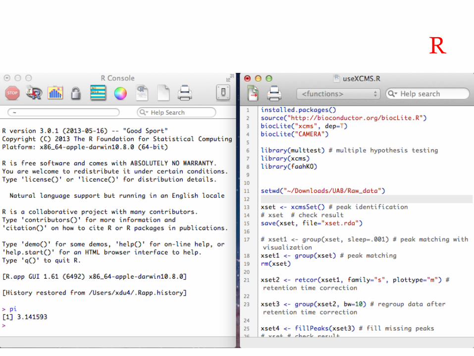
• Take a look at the xcmsSet object:

Peak identification (IV)
20
• The default parameters should work acceptably in most cases. – Default peak detection method: matched filter – Alternative approach: centWave for high resolution MS data
• However, a number of parameters might need to be optimized for particular instruments or experimental conditions. – Matched filtration: model peak width, m/z step size for creating
extracted ion base peak chromatograms (EIBPC), the algorithm to create EIBPC, …
– centWave: ppm, peak width range, …
• To be explained in the next section “Parameter set-up …” by Paul

Matching peaks across samples
21
• After peak identification, peaks representing the same analyte across samples must be placed into groups.
• This is accomplished with the group() method.
• There are several grouping parameters to consider optimizing for your chromatography and mass spectrometer (to be explained by Paul).

Retention time correction (I)
22
• XCMS uses peak groups to identify and correct drifts in retention time from run to run.
• Only well-behaved peak groups are used: missing the peak from at most one sample and having at most one extra peak.
• These parameters can be changed with the missing and extra arguments.
• For each of those well-behaved groups, XCMS calculates a median retention time and, for every sample, a deviation from that median.
Retention time correction (II)
23
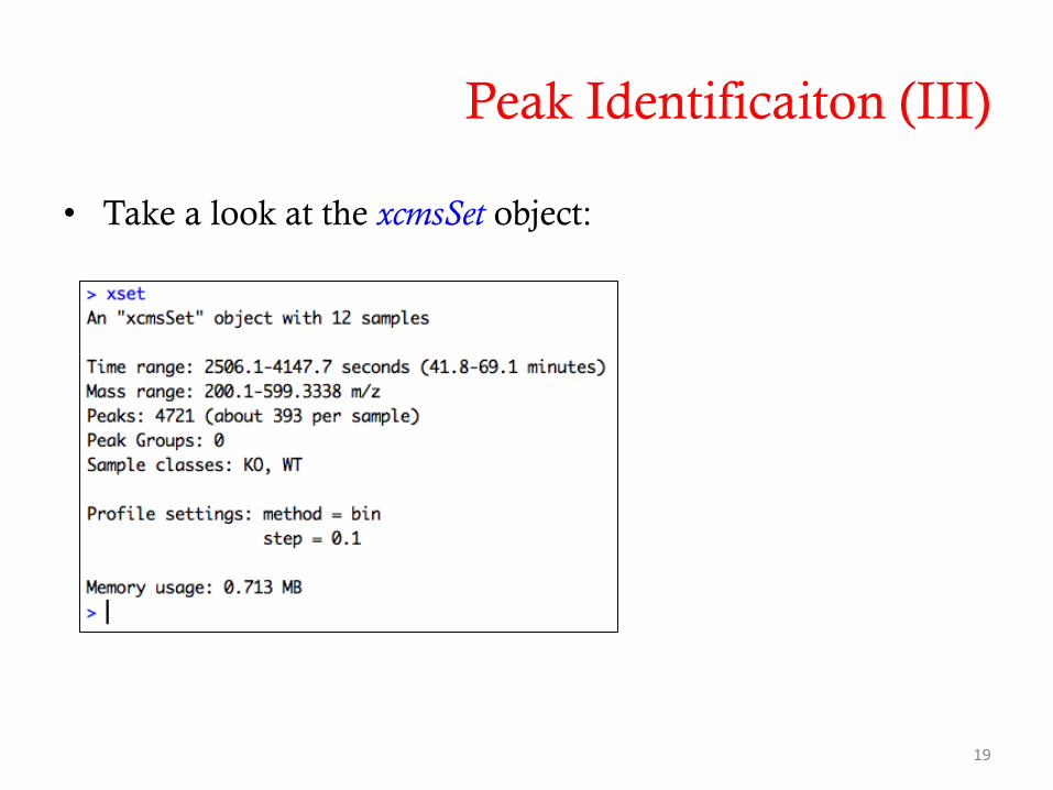
• Within a sample, the observed deviation generally changes over time in a nonlinear fashion.
• Those changes are modeled using a local polynomial regression technique.
• Retention time correction is performed by the retcor() method.
• The plottype argument produces the plot on the next slide.

Retention time correction (III)
24

Retention time correction (IV)
25
• Use the plot to supervise the algorithm. The plot includes data points used for regression and the resulting deviation profiles.
• The plot also shows the distribution of peak groups across retention time.

Retention time correction (V)
26
• After retention time correction, the initial peak grouping becomes invalid.
• Peak re-grouping is needed.
• This iteration of peak grouping and alignment can be repeated in an iterative fashion.

Filling in missing peaks (I)
27
• Peaks could be missing due to imperfection in peak identification or because an analyte was not present in a sample.
• For missing peaks that correspond to analytes that are actually in the sample, the missing data points can be filled in by re-reading the raw data files and integrating them in the regions of the missing peaks.
• This is performed using the fillPeaks() method.

Filling in missing peaks (II)
28

Analyzing and visualizing results (I)
29
• A report showing the most statistically significant differences in analyte intensities can be generated with the diffreport() method.
• Results are stored in two folders and one spread sheet file.

Analyzing and visualizing results (II)
30
Extracted ion chromatograms for significant ions
001.png 006.png 010.png

Analyzing and visualizing results (III)
31
001.png 006.png 010.png
Box plots for significant ions

Analyzing and visualizing results (IV)
32
example.tsv (column A to K)

Analyzing and visualizing results (V)
33
example.tsv (column O to AA)

Going back to the raw data (I)
34
mzmed = 300.2, rtmed = 3390.3 sec = 56.5 min

Going back to the raw data (II)
35

Visualize raw data
36
• Mass spectrometer vendors save data in proprietary formats.
• These data files can be converted to open data formats for easy reading.
• Software tools to do the conversion: msConvert

msConvert (I)
37
• Part of ProteoWizard • Read from
– mzML, mzXML, MGF – Agilent, Bruker, Thermo, Waters, ABSciex
• Write to
– open formats – perform various filters and transformations
• http://proteowizard.sourceforge.net/ • For Windows, msConvertGUI is available for easy file
conversion.

msConvert (II)
38

Raw data visualization
39
• Software tool: Insilicos Viewer – View raw MS data in formats including mzXML,
mzData, mzML, and ANDI CDF
– http://insilicos.com/products/insilicos-viewer-1 – Quick demo

Run all the commands
40

41
Thank you!


