
Basic template for the development of ISO and ISO/IEC...
460
ISO/IEC PDTR 15938-8 INTERNATIONAL ORGANIZATION FOR STANDARDIZATION ORGANISATION INTERNATIONALE NORMALISATION ISO/IEC JTC 1/SC 29/WG 11 CODING OF MOVING PICTURES AND AUDIO ISO/IEC JTC 1/SC 29/WG 11N4360 July 2001 Source: Video/MDS Subgroup Title: Text of ISO/IEC 15938-8 PDTR (Extraction and Use of MPEG-7 Descriptions) Status: Final Editors: P. van Beek, A. B. Benitez, L. Cieplinski, J. Heuer, W. Kim, J. Martinez, J.-R. Ohm, M. Pickering, P. Salembier, Y. Shibata, J. Smith, T. Walker A. Yamada 1
Transcript of Basic template for the development of ISO and ISO/IEC...

ISO/IEC PDTR 15938-8
INTERNATIONAL ORGANIZATION FOR STANDARDIZATIONORGANISATION INTERNATIONALE NORMALISATION
ISO/IEC JTC 1/SC 29/WG 11
CODING OF MOVING PICTURES AND AUDIO
ISO/IEC JTC 1/SC 29/WG 11N4360July 2001
Source: Video/MDS Subgroup
Title: Text of ISO/IEC 15938-8 PDTR (Extraction and Use of MPEG-7 Descriptions)
Status: Final
Editors: P. van Beek, A. B. Benitez, L. Cieplinski, J. Heuer, W. Kim, J. Martinez, J.-R. Ohm, M. Pickering, P. Salembier, Y. Shibata, J. Smith, T. Walker A. Yamada
1

ISO/IEC PDTR 15938-8
ISO/IEC JTC 1/SC 29 M XXXXDate: 2001-10-08
ISO/IEC PDTR 15938-8
ISO/IEC JTC 1/SC 29/WG 11
Secretariat: XXXX
Information Technology — Multimedia Content Description Interface — Part 8: Extraction and use of MPEG-7 descriptionsTitre — Titre — Partie n: Titre de la partie
Warning
This document is not an ISO International Standard. It is distributed for review and comment. It is subject to change without notice and may not be referred to as an International Standard.
Recipients of this document are invited to submit, with their comments, notification of any relevant patent rights of which they are aware and to provide supporting documentation.
Document type: International standardDocument subtype: if applicableDocument stage: (30) CommitteeDocument language: E
2

ISO/IEC PDTR 15938-8
Copyright notice
This ISO document is a working draft or committee draft and is copyright-protected by ISO. While the reproduction of working drafts or committee drafts in any form for use by participants in the ISO standards development process is permitted without prior permission from ISO, neither this document nor any extract from it may be reproduced, stored or transmitted in any form for any other purpose without prior written permission from ISO.
Requests for permission to reproduce this document for the purpose of selling it should be addressed as shown below or to ISO’s member body in the country of the requester:
[Indicate :the full addresstelephone numberfax numbertelex numberand electronic mail address
as appropriate, of the Copyright Manager of the ISO member body responsible for the secretariat of the TC or SC within the framework of which the draft has been prepared]
Reproduction for sales purposes may be subject to royalty payments or a licensing agreement.
Violators may be prosecuted.
3
ISO/IEC PDTR 15938-8
Contents
INTERNATIONAL ORGANIZATION FOR STANDARDIZATION 11 Scope 171.1 Organization of the document 172 References 173 Terms and definitions193.1 Conventions 193.2 Terminology 193.3 Symbols (and abbreviated terms) 244 MDS tools 264.1 Schema tools 264.2 Basic datatypes 404.3 Linking, identification and localization tools 464.4 Basic description tools 534.5 Media description tools 974.6 Creation and production description tools 1054.7 Usage description tools 1094.8 Structure description tools 1124.9 Semantics description tools 1754.10 Navigation and access tools 2034.11 Content organization tools 2474.12 User interaction tools2715 Visual tools 2875.1 Basic visual tools 2875.2 Color description tools 3045.3 Texture description tools 3205.4 Shape description tools 3305.5 Motion description tools 3455.6 Localization tools 3665.7 Other visual tools 373Annex A Patent Statements 383
4

ISO/IEC PDTR 15938-8
5

ISO/IEC PDTR 15938-8
Foreword
ISO (the International Organization for Standardization) and IEC (the International Electrotechnical Commission) form the specialized system for worldwide standardization. National bodies that are members of ISO or IEC participate in the development of International Standards through technical committees established by the respective organization to deal with particular fields of technical activity. ISO and IEC technical committees collaborate in fields of mutual interest. Other international organizations, governmental and non-governmental, in liaison with ISO and IEC, also take part in the work.
International Standards are drafted in accordance with the rules given in the ISO/IEC Directives, Part 3.
In the field of information technology, ISO and IEC have established a joint technical committee, ISO/IEC JTC 1. Draft International Standards adopted by the joint technical committee are circulated to national bodies for voting. Publication as an International Standard requires approval by at least 75 % of the national bodies casting a vote.
Attention is drawn to the possibility that some of the elements of this part of ISO/IEC 15938 may be the subject of patent rights. ISO and IEC shall not be held responsible for identifying any or all such patent rights.
International Standard ISO/IEC 15938-5 was prepared by Joint Technical Committee ISO/IEC JTC 1, JTC, Subcommittee SC 29.
This second/third/... edition cancels and replaces the first/second/... edition (), [clause(s) / subclause(s) / table(s) / figure(s) / annex(es)] of which [has / have] been technically revised.
ISO/IEC 15938 consists of the following parts, under the general title Information Technology — Multimedia Content Description Interface:
Part 1: Systems
Part 2: Description definition language
Part 3: Visual
Part 4: Audio
Part 5: Multimedia description schemes
Part 6: Reference software
Part 7: Conformance testing
Part 8: Extraction and use of MPEG-7 descriptions
6

ISO/IEC PDTR 15938-8
Introduction
This standard, also known as "Multimedia Content Description Interface," provides a standardized set of technologies for describing multimedia content. The standard addresses a broad spectrum of multimedia applications and requirements by providing a metadata system for describing the features of multimedia content.
The following are specified in this standard:
Description Schemes (DS) describe entities or relationships pertaining to multimedia content. Description Schemes specify the structure and semantics of their components, which may be Description Schemes, Descriptors, or datatypes.
Descriptors (D) describe features, attributes, or groups of attributes of multimedia content.
Datatypes are the basic reusable datatypes employed by Description Schemes and Descriptors
Systems tools support delivery of descriptions, multiplexing of descriptions with multimedia content, synchronization, file format, and so forth.
This standard is subdivided into eight parts:
Part 1 – Systems: specifies the tools for preparing descriptions for efficient transport and storage, compressing descriptions, and allowing synchronization between content and descriptions.
Part 2 – Description definition language: specifies the language for defining the standard set of description tools (DSs, Ds, and datatypes) and for defining new description tools.
Part 3 – Visual: specifies the description tools pertaining to visual content.
Part 4 – Audio: specifies the description tools pertaining to audio content.
Part 5 – Multimedia description schemes: specifies the generic description tools pertaining to multimedia including audio and visual content.
Part 6 – Reference software: provides a software implementation of the standard.
Part 7 – Conformance testing: specifies the guidelines and procedures for testing conformance of implementations of the standard.
Part 8 – Extraction and use of MPEG-7 descriptions: provides guidelines and examples of the extraction and use of descriptions.
7

ISO/IEC PDTR 15938-8
Information technology — Multimedia content description interface — Part 8: Extraction and use of MPEG-7 descriptions
1 Scope
1.1 Organization of the document
This International Standard specifies a metadata system for describing multimedia content. This document gives examples of extraction and use of descriptions using Description Schemes, Descriptors, and datatypes specified in ISO/IEC 15938. The following set of subclauses are provided for each description tool, where optional subclauses are indicated as (optional):
Informative examples (optional): provides informative examples that illustrate the instantiation of the description tool in creating descriptions.
Extraction (optional): provides informative examples that illustrate the extraction of descriptions from multimedia content.
Use (optional): provides informative examples that illustrate the use of descriptions.
2 References
The following normative documents contain provisions which, through reference in this text, constitute provisions of this part of ISO/IEC 15938. At the time of publication of this document, the specific editions indicated below were valid. However, parties to agreements based on this part of ISO/IEC 15938 are encouraged to investigate the possibility of applying the most recent editions of the normative documents indicated below. For undated references, the latest edition of the normative document referred to applies. Members of ISO and IEC maintain registers of currently valid International Standards. The Telecommunication Standardization Bureau maintains a list of currently valid ITU-T Recommendations.
ISO 8601, Data elements and interchange formats -- Information interchange -- Representation of dates and times.
ISO 639, Code for the representation of names of languages.
ISO 3166-1, Codes for the representation of names of countries and their subdivisions -- Part 1: Country codes.
ISO 3166-2, Codes for the representation of names of countries and their subdivisions -- Part 2: Country subdivision code.
Note: The current list of valid ISO3166-1 country and ISO3166-2 region codes is maintained by the official maintenance authority Deutsches Institut für Normung. Information on the current list of valid region and country codes can be found at http://www.din.de/gremien/nas/nabd/iso3166ma/index.html.
ISO 4217, Codes for the representation of currencies and funds.
1

ISO/IEC PDTR 15938-8
Note (informative): The current list of valid ISO 4217 currency codes is maintained by the official maintenance authority British Standards Institution (http://www.bsi-global.com/iso4217currency).
XML, Extensible Markup Language (XML) 1.0, October 2000.
XML Schema, W3C Recommendation, 2 May 2001.
XML Schema Part 0: Primer, W3C Recommendation, 2 May 2001.
XML Schema Part 1: Structures, W3C Recommendation, 2 May 2001.
XML Schema Part 2: Datatypes, W3C Recommendation 2 May 2001.
xPath, XML Path Language, W3C Recommendation, 16 November 1999.
Note (informative): These documents are maintained by the W3C (http://www.w3.org). The relevant documents can be obtained as follows:
o Extensible Markup Language (XML) 1.0 (Second Edition), 6 October 2000, http://www.w3.org/TR/2000/REC-xml-20001006
o XML Schema: W3C Recommendation, 2 May 2001, http://www.w3.org/XML/Schema
XML Schema Part 0: Primer, W3C Recommendation, 2 May 2001, http://www.w3.org/TR/xmlschema-0/
XML Schema Part 1: Structures, W3C Recommendation, 2 May 2001, http://www.w3.org/TR/xmlschema-1/
XML Schema Part 2: Datatypes, W3C Recommendation 2 May 2001, http://www.w3.org/TR/xmlschema-2/
o xPath, XML Path Language, W3C Recommendation, 16 November 1999, http://www.w3.org/TR/1999/REC-xpath-19991116.
RFC 2045 Multipurpose Internet Mail Extensions (MIME) Part One: Format of Internet Message Bodies.
RFC 2046 Multipurpose Internet Mail Extensions (MIME) Part Two: Media Types.
RFC 2048, Multipurpose Internet Mail Extensions (MIME) Part Four: Registration Procedures.
RFC2045-CHARSETS. Registered Character set codes of RFC2045.
RFC2046-MIMETYPES. Registered Mimetypes of RFC2046.
Note (informative): The relevant lists can be obtained as follows:
o MIMETYPES. The current list of registered mimetypes, as defined in RFC2046, RFC2048, is maintained by IANA (Internet Assigned Numbers Authority). It is available from ftp://ftp.isi.edu/in-notes/iana/assignments/media-types/media-types/
o CHARSETS. The current list of registered character set codes, as defined in RFC2045 and RFC2048 is maintained by IANA (Internet Assigned Numbers Authority). It is available from ftp://ftp.isi.edu/in-notes/iana/assignments/character-sets.
2

ISO/IEC PDTR 15938-8
3 Terms and definitions
3.1 Conventions
3.1.1 Description tools
This part of ISO/IEC 15938 specifies the multimedia description tools as follows:
Description Scheme (DS) – a description tool that describes entities or relationships pertaining to multimedia content. DSs specify the structure and semantics of their components, which may be Description Schemes, Descriptors, or datatypes.
Descriptor (D) – a description tool that describes a feature, attribute, or group of attributes of multimedia content.
Datatype – a basic reusable datatype employed by Description Schemes and Descriptors.
Description Tool (or tool) – refers to a Description Scheme, Descriptor, or Datatype.
3.1.2 Naming convention
In order to specify the multimedia description tools, this part of ISO/IEC 15938 uses constructs provided by the Description Definition Language (DDL) specified in ISO/IEC 15938-2, such as "element", "attribute", "simpleType" and "complexType". The names associated to these constructs are created on the basis of the following conventions:
If the name is composed of multiple words, the first letter of each word is capitalized, with the exception that the capitalization of the first word depends on the type of construct as follows:
Element naming: the first letter of the first word is capitalized (e.g. TimePoint element of TimeType).
Attribute naming: the first letter of the first word is not capitalized (e.g. timeUnit attribute of IncrDurationType).
complexType naming: the first letter of the first word is capitalized, and the suffix "Type" is used at the end of the name (e.g. PersonType).
simpleType naming: the first letter of the first word is not capitalized, the suffix "Type" may be used at the end of the name (e.g. timePointType).
Note that when referencing a complexType or simpleType in the definition of a description tool, the "Type" suffix is not used. For instance, the text refers to the "Time datatype" (instead of "TimeType datatype"), to the "MediaLocator D" (instead of "MediaLocatorType D") and to the "Person DS" (instead of PersonType DS).
3.2 Terminology
For the purposes of this part of ISO/IEC 15938, the following terms and definitions apply.
3.2.1 Schema-related terminology
3.3.1.1AttributeA field of a description tool which is of simple type.
3.3.1.2Base typeA type that serves as the root type of a derivation hierarchy for other types.
3

ISO/IEC PDTR 15938-8
3.3.1.3DatatypeA primitive reusable type employed by Description Schemes and Descriptors.
3.3.4Derived typeA type that is defined in terms of extension or restriction of other types.
3.3.1.5DescriptionAn instantiation of one or more description tools.
3.3.1.6Description SchemeA description tool that describes entities or relationships pertaining to multimedia content. Description Schemes specify the structure and semantics of their components, which may be Description Schemes, Descriptors, or datatypes.
3.3.1.7Description ToolA Description Scheme, Descriptor, or datatype.
3.3.1.8Descriptor3.3.10InstantiationAssignment of values to the fields (elements, attributes) of one or more description tools.
3.3.1.10ElementA field of a description tool which is of complex type.
3.3.1.11SchemaThe set of related description tools, for example, those specified in ISO/IEC 15938.
3.3.1.12TypeThe format used for collection of letters, digits, and/or symbols, to depict values of an element or attribute of description tool. A type consists of a set of distinct values, a set of lexical representations, and a set of facets that characterize properties of the value space, individual values, or lexical items.
3.2.2 Content-related terminology
3.3.2.1AbstractionA secondary representation that is created from or is related to the content. For example, a summary of a video or a model of a feature.
3.3.2.2AcquisitionThe process of acquiring audio or visual data from a source.
3.3.2.3ActionA semantically identifiable behavior of an object or group of objects, for example, a soccer player kicking ball.
3.3.2.4AgentA person, organization, or group of persons.
4

ISO/IEC PDTR 15938-8
3.3.2.5AudioTime-varying data or signal intended for listening or hearing. Also, related to the aural modality.
3.3.2.6Audio-visualcontent consisting of both audio and video data.
3.3.2.7AutomaticProcessing of multimedia data, content, or metadata by means of computer, hardware, or other software device.
3.3.2.8Classification SchemeA list of defined terms and their meanings.
3.3.2.9ContentMultimedia contentA representation of the information contained in or related to multimedia data in a formalized manner suitable for interpretation by human means. Content refers to the data and the metadata.
3.3.2.10CopyrightA right that establishes the ownership of data, content, or metadata.
3.3.2.11DataEssenceMultimedia DataA representation of multimedia in a formalized manner suitable for communication, interpretation, or processing by automatic means.
3.3.2.12EditingThe process of combining, extracting, and refining multimedia data.
3.3.2.13EntityAny concrete or abstract thing of interest related to the multimedia content.
3.3.2.14EventA noteworthy occurrence that happens at a point in time or during a temporal interval. Alternatively used as a change in state.
3.3.2.15FeatureA distinctive characteristic of multimedia content that signifies something to a human observer, such as the "color" or "texture" of an image.
3.3.2.16FilteringA process for selecting multimedia content that satisfies certain criteria. This process may include ranking the content according to the extent that it satisfies the criteria.
3.3.2.17FormatThe characteristics of the stored or physical representation of the data.
5

ISO/IEC PDTR 15938-8
3.3.2.18FrameA single image from a video.
3.3.2.19Image2D spatially-varying visual data acquired from a visual source.
3.3.2.20Key frameA representative frame of a video or a segment.
3.3.2.21LocatorSpecifies the location or address of multimedia data or a segment.
3.3.2.22ModelA parametric or statistical representation of multimedia content or features.
3.3.2.23ManualProcessing of multimedia data, content, or metadata by human means.
3.3.2.24MetadataThe information and documentation which makes multimedia data understandable and shareable to users over time.
3.3.2.25MultimediaData comprising one or modalities, such as images, audio, video, 3D models, ink content, and so forth.
3.3.2.26NavigationA process by which a user accesses multimedia content and steers a course through the content in a controlled manner.
3.3.2.27ObjectAn object with a physical representation in the natural world.
3.3.2.28RegionA spatial unit of multimedia, for example, a 2D spatial region of an image, or a moving region of video.
3.3.2.29RelationAny association among entities.
3.3.2.30RightsInformation that determines the ownership and terms of use of multimedia data, content, or metadata. Refers to Intellectual Property Rights, Copyrights, and the Access Rights.
6

ISO/IEC PDTR 15938-8
3.3.2.31SceneAn episode or sequence of events representing continuous action in one location.
3.3.2.32SearchA process for searching multimedia content that satisfies certain criteria. This process may include ranking the content according to the extent that it satisfies the criteria.
3.3.2.33SegmentA spatial or temporal unit of multimedia, for example, a temporal segment of video, or a segment of an image.
3.3.2.34SemanticsInformation relating to the underlying meaning or understanding of multimedia content. Alternatively, refers to the specification of the meaning of description tools.
3.3.2.35SummaryAn abstraction of multimedia content that summarizes the content.
3.3.2.36UserAn end-user or consumer of multimedia content.
3.3.2.37User PreferencesThe preferences of a user pertaining to multimedia content. This includes the user's tastes, likes and dislikes with respect to the content and its properties, as well as preferences with respect to the consumption process.
3.3.2.38Usage HistoryA history of actions that a user of multimedia content has carried out over a certain period of time, such as recording a specific piece of content, or playing back recorded content at a specific time.
3.3.2.39VariationAn alternative version of multimedia content., which may be derived through transcoding, summarization, translation, reduction, and so forth.
3.3.2.40VideoA space- and time-varying visual data or signal intended for viewing; commonly represented as a discrete sequence of images or frames.
3.3.2.41ViewA portion of an image, video or audio signal, defined in terms of a partition. A partition is a multi-dimensional region defined in the space, time and/or frequency plane.
3.3.2.42VisualRelated to the visual modality.
3.3.2.43View DecompositionAn organized set of views that provides a structured decomposition of an image, video or audio signal in multi-dimensional space, time and/or frequency.
7
ISO/IEC PDTR 15938-8
3.3 Symbols (and abbreviated terms)
For the purposes of this part of ISO/IEC 15938, the symbols and abbreviated terms given in the following apply:
AV: Audio-visual
CIF: Common Intermediate Format
CS: Classification Scheme
D: Descriptor
Ds: Descriptors
DCT: Discrete Cosine Transform
DDL: Description Definition Language
DS: Description Scheme
DSs: Description Schemes
IANA: Internet Assigned Numbers Authority
IETF: Internet Engineering Task Force
IPMP: Intellectual Property Management and Protection
ISO: International Organization for Standardization
JPEG: Joint Photographic Experts Group
MDS: Multimedia Description Scheme
MPEG: Moving Picture Experts Group
MPEG-2: Generic coding of moving pictures and associated audio information (see ISO/IEC 13818)
MPEG-4: Coding of audio-visual objects (see ISO/IEC 14496)
MPEG-7: Multimedia Content Description Interface Standard (see ISO/IEC 15938)
MP3: MPEG-2 layer 3 audio coding
QCIF: Quarter Common Intermediate Format
SMPTE: Society of Motion Picture and Television Engineers
TZ: Time Zone
TZD: Time Zone Difference
URI: Uniform Resource Identifier (see RFC 2396)
URL: Uniform Resource Locator (see RFC 2396)
W3C: World Wide Web Consortium
XML: Extensible Markup Language
8

ISO/IEC PDTR 15938-8
9

ISO/IEC PDTR 15938-8
4 MDS tools
4.1 Schema tools
4.1.1 Introduction
This clause specifies the schema tools that facilitate the making of descriptions. The following description tools are specified: (1) the base type hierarchy of the description tools defined in ISO/IEC 15938, (2) the root element, (3) the top-level tools, (4) the multimedia content entity tools, (5) package tool, and (6) description metadata tool. The functionality of these tools is given as follows:
Table 1: Overview of Schema Tools.Tool Functionality
Base types Forms the type hierarchy for description tools.
Root element Describes the initial wrapper or root element of descriptions.
Top-level tools Describes the elements that follow the root element in descriptions.
Multimedia content entity tools
Describes different types of multimedia content such as images, video, audio, mixed multimedia, collections, and so forth.
Package tool Describes an organization or packaging of description tools.
Description metadata tool Describes metadata about descriptions.
.
4.1.2 Base types
No additional informative material for extraction and use is provided.
4.1.3 Root element
4.1.3.1 Root element examples
The following example shows the use of the root element for describing an instance of the ScalableColor D (defined in ISO/IEC 15398-3) using DescriptionUnit.
<Mpeg7><DescriptionMetadata>
<Version>1.0</Version><PrivateIdentifier>descriptionUnitExample</PrivateIdentifier>
</DescriptionMetadata><DescriptionUnit xsi:type="ScalableColorType" numOfCoeff="16"
numOfBitplanesDiscarded="0"><Coeff> 1 2 3 4 5 6 7 8 9 0 1 2 3 4 5 6 </Coeff>
</DescriptionUnit></Mpeg7>
The following example shows the use of root element for describing an image using Description.
<Mpeg7><DescriptionMetadata>
10

ISO/IEC PDTR 15938-8
<Confidence>1.0</Confidence><Version>1.1</Version><LastUpdate>2001-09-20T03:20:25+09:00</LastUpdate><PublicIdentifier>
<IDOrganization><Name>ISO</Name>
</IDOrganization><IDName>
<Name>International Organization of Standardization</Name></IDName><UniqueID>098f2470-bae0-11cd-b579-08002b30bfeb</UniqueID>
</PublicIdentifier><PrivateIdentifier>completeDescriptionExample</PrivateIdentifier><Creator>
<Role href="creatorCS"><Name>Creator</Name><Role><Person>
<Name><GivenName>Yoshiaki</GivenName><FamilyName>Shibata</FamilyName>
</Name></Person>
</Creator><CreationLocation>
<Country>jp</Country><AdministrativeUnit>Tokyo</AdministrativeUnit>
</CreationLocation><CreationTime>2000-10-10T19:45:00+09:00</CreationTime><Instrument>
<Tool><Name>Wizzo Extracto ver. 2</Name>
</Tool><Setting name="sensitivity" value="0.5"/>
</Instrument><Rights> RID# </Rights>
</DescriptionMetadata><Description xsi:type="ContentEntityType">
<MultimediaContent xsi:type="ImageType"><Image>
<!-- more elements here --></Image>
</MultimediaContent></Description>
</Mpeg7>
4.1.4 Top-level types
4.1.4.1 Complete description types
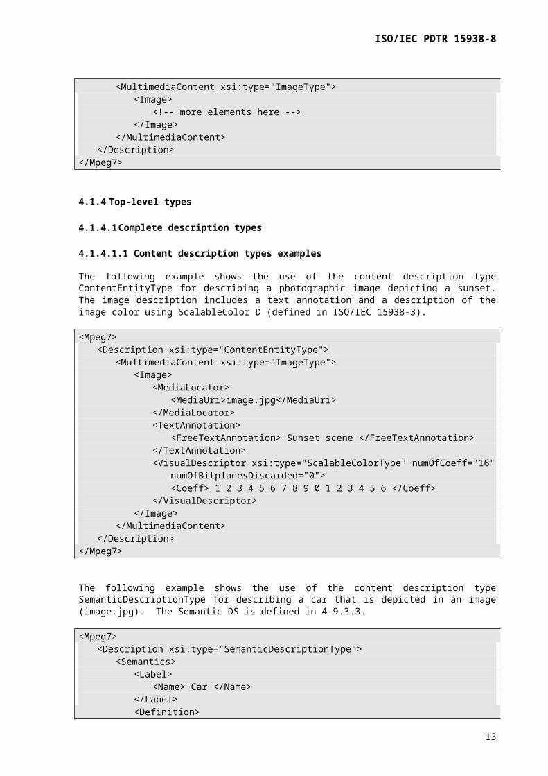
4.1.4.1.1 Content description types examples
The following example shows the use of the content description type ContentEntityType for describing a photographic image depicting a sunset. The image description includes a text annotation and a description of the image color using ScalableColor D (defined in ISO/IEC 15938-3).
<Mpeg7><Description xsi:type="ContentEntityType">
<MultimediaContent xsi:type="ImageType"><Image>
<MediaLocator>
11
ISO/IEC PDTR 15938-8
<MediaUri>image.jpg</MediaUri></MediaLocator><TextAnnotation>
<FreeTextAnnotation> Sunset scene </FreeTextAnnotation></TextAnnotation><VisualDescriptor xsi:type="ScalableColorType" numOfCoeff="16"
numOfBitplanesDiscarded="0"><Coeff> 1 2 3 4 5 6 7 8 9 0 1 2 3 4 5 6 </Coeff>
</VisualDescriptor></Image>
</MultimediaContent></Description>
</Mpeg7>
The following example shows the use of the content description type SemanticDescriptionType for describing a car that is depicted in an image (image.jpg). The Semantic DS is defined in 4.9.3.3.
<Mpeg7><Description xsi:type="SemanticDescriptionType">
<Semantics><Label>
<Name> Car </Name></Label><Definition>
<FreeTextAnnotation>Four wheel motorized vehicle
</FreeTextAnnotation></Definition><MediaOccurrence>
<MediaLocator><MediaUri> image.jpg </MediaUri>
</MediaLocator></MediaOccurrence>
</Semantics></Description>
</Mpeg7>
The following example shows the use of the content description type ModelDescriptionType for describing a collection model of "sunsets" that contains two images depicting sunset scenes. The CollectionModel DS is defined in 4.11.5.2.
<Mpeg7><Description xsi:type="ModelDescriptionType">
<Model xsi:type="CollectionModelType" confidence="0.75" reliability="0.5"
function="described"><Label>
<Name>Sunsets</Name></Label><Collection xsi:type="ContentCollectionType">
<Content xsi:type="ImageType"><Image>
<MediaLocator xsi:type="ImageLocatorType"><MediaUri>sunset1.jpg</MediaUri>
</MediaLocator></Image>
</Content><Content xsi:type="ImageType">
12

ISO/IEC PDTR 15938-8
<Image><MediaLocator xsi:type="ImageLocatorType">
<MediaUri>sunset2.jpg</MediaUri></MediaLocator>
</Image></Content>
</Collection></Model>
</Description></Mpeg7>
The following example shows the use of the content description type SummaryDescriptionType for describing a hierarchical summary of video. The hierarchical summary has two levels: level 0 consists of three summary segments, and level 1 consists of one summary segment. The HierarchicalSummary DS is defined in 4.10.2.3.
<Mpeg7><Description xsi:type="SummaryDescriptionType">
<Summarization><Summary xsi:type="HierarchicalSummaryType"
components="keyVideoClips" hierarchy="dependent"><SourceLocator>
<MediaUri>file://disk/video001.mpg</MediaUri></SourceLocator><SummarySegmentGroup level="0">
<SummarySegment> <!-- segment #1 at level 0 --> </SummarySegment>
<SummarySegment> <!-- segment #2 at level 0 --> </SummarySegment>
<SummarySegment> <!-- segment #3 at level 0 --> </SummarySegment>
<SummarySegmentGroup level="1"><SummarySegment> <!-- segment #1 at level 1 -->
</SummarySegment></SummarySegmentGroup>
</SummarySegmentGroup></Summary>
</Summarization></Description>
</Mpeg7>
The following example shows the use of the content description type ViewDescriptionType for describing a spatial view of an image, which corresponds to the upper-right quarter of the image. The SpaceView DS is defined in 4.10.3.5.
<Mpeg7><Description xsi:type="ViewDescriptionType">
<View xsi:type="SpaceViewType"><Target>
<ImageSignal><MediaLocator>
<MediaUri> view.jpg </MediaUri></MediaLocator>
</ImageSignal></Target><Source>
<ImageSignal><MediaLocator>
13

ISO/IEC PDTR 15938-8
<MediaUri> image.jpg </MediaUri></MediaLocator>
</ImageSignal></Source><SpacePartition>
<Origin xOrigin="left" yOrigin="top"/><Start xsi:type="SignalPlaneFractionType" x="0.5" y="0"/><End xsi:type="SignalPlaneFractionType" x="0.5" y="0.5"/>
</SpacePartition></View>
</Description></Mpeg7>
The following example shows the use of the content description type VariationDescriptionType for describing an image that is a variation of a video in which the image has been extracted from the video. The VariationSet DS is defined in 4.10.4.1.
<Mpeg7><Description xsi:type="VariationDescriptionType">
<VariationSet><Source xsi:type="mpeg7:VideoType">
<Video><MediaLocator>
<MediaUri>file://video-A.mpg</MediaUri></MediaLocator>
</Video></Source><Variation fidelity="0.85" priority="1">
<Content xsi:type="ImageType"><Image>
<MediaLocator><MediaUri>file://image-B.jpg</MediaUri>
</MediaLocator></Image>
</Content><VariationRelationship>extraction</VariationRelationship>
</Variation></VariationSet>
</Description></Mpeg7>
4.1.4.2 Content management types
4.1.4.2.1 Content management types example
The following example shows the use of the content management type UserDescriptionType for describing the user preferences of a user of a multimedia system. The UserPreferences DS is defined in 4.12.2.2.
<Mpeg7><Description xsi:type="UserDescriptionType">
<User xsi:type="PersonType"><Name xml:lang="en">
<GivenName> John </GivenName><FamilyName> Smith </FamilyName>
</Name></User><UserPreferences>
14
ISO/IEC PDTR 15938-8
<UserIdentifier> <Name> jrsmith </Name> </UserIdentifier> <FilteringAndSearchPreferences> <!-- more elements here --> </FilteringAndSearchPreferences>
</UserPreferences></Description>
</Mpeg7>
The following example shows the use of the content management type MediaDescriptionType for describing the media information of a news video. The MediaInformation DS is defined in 4.5.2.1.
<Mpeg7><Description xsi:type="MediaDescriptionType">
<MediaInformation id="news1_media"><MediaIdentification>
<EntityIdentifier organization="MPEG" type="MPEG7ContentSetId">
mpeg7_content:news1</EntityIdentifier>
<VideoDomain href="urn:mpeg:mpeg7:cs:VideoDomainCS:2001:1.2"><Name xml:lang="en">Natural</Name>
</VideoDomain></MediaIdentification><MediaProfile>
<MediaFormat><Content href="MPEG7ContentCS">
<Name>audiovisual</Name></Content><Medium href="urn:mpeg:mpeg7:cs:MediumCS:2001:1.1">
<Name xml:lang="en">CD</Name></Medium><FileFormat href="urn:mpeg:mpeg7:cs:FileFormatCS:2001:3">
<Name xml:lang="en">mpeg</Name></FileFormat><FileSize>666478608</FileSize><VisualCoding>
<Format href="urn:mpeg:mpeg7:cs:VisualCodingFormatCS:2001:1"
colorDomain="color"><Name xml:lang="en">MPEG-1 Video</Name>
</Format><Pixel aspectRatio="0.75" bitsPer="8"/><Frame height="288" width="352" rate="25"/>
</VisualCoding></MediaFormat>
</MediaProfile></MediaInformation>
</Description></Mpeg7>
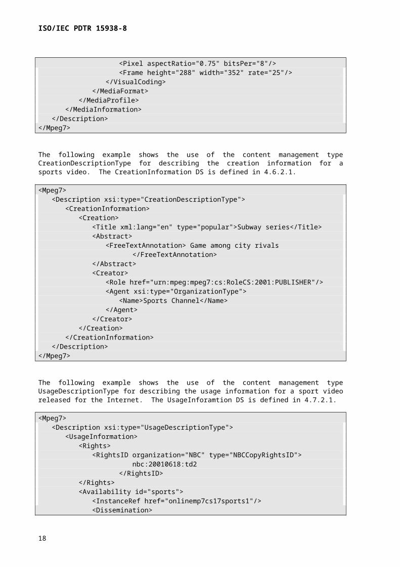
The following example shows the use of the content management type CreationDescriptionType for describing the creation information for a sports video. The CreationInformation DS is defined in 4.6.2.1.
<Mpeg7><Description xsi:type="CreationDescriptionType">
15

ISO/IEC PDTR 15938-8
<CreationInformation><Creation>
<Title xml:lang="en" type="popular">Subway series</Title><Abstract>
<FreeTextAnnotation> Game among city rivals </FreeTextAnnotation>
</Abstract><Creator>
<Role href="urn:mpeg:mpeg7:cs:RoleCS:2001:PUBLISHER"/><Agent xsi:type="OrganizationType">
<Name>Sports Channel</Name></Agent>
</Creator></Creation>
</CreationInformation></Description>
</Mpeg7>
The following example shows the use of the content management type UsageDescriptionType for describing the usage information for a sport video released for the Internet. The UsageInforamtion DS is defined in 4.7.2.1.
<Mpeg7><Description xsi:type="UsageDescriptionType">
<UsageInformation><Rights>
<RightsID organization="NBC" type="NBCCopyRightsID">nbc:20010618:td2
</RightsID></Rights><Availability id="sports">
<InstanceRef href="onlinemp7cs17sports1"/><Dissemination>
<Format href="urn:mpeg:mpeg7:cs:DisseminationFormatCS:2001:4">
<Name xml:lang="en">Internet</Name></Format><Location>
<Region>us</Region></Location>
</Dissemination><AvailabilityPeriod type="payPerUse">
<TimePoint>2001-06-16T21:00+01:00</TimePoint><Duration>PT30M</Duration>
</AvailabilityPeriod></Availability>
</UsageInformation></Description>
</Mpeg7>
The following example shows the use of the content management type ClassificationSchemeDescriptionType for describing a classification scheme for audio domain. The ClassificationScheme DS is defined in 4.4.4.1.
<Mpeg7><Description xsi:type="ClassificationSchemeDescriptionType">
<ClassificationScheme uri="urn:mpeg:mpeg7:cs:MyAudioDomainCS"
16

ISO/IEC PDTR 15938-8
domain="//MediaInformation/MediaProfile/MediaIdentification/AudioDomain"><Header xsi:type="DescriptionMetadataType">
<Version>1.0</Version></Header><Term termID="1">
<Name xml:lang="en">Source</Name><Definition xml:lang="en">Type of audio source</Definition><Term termID="1.1">
<Name xml:lang="en">Synthetic</Name></Term><Term termID="1.2">
<Name xml:lang="en">Natural</Name></Term>
</Term></ClassificationScheme>
</Description></Mpeg7>
4.1.4.3 Multimedia content entity description tools
4.1.4.3.1 Multimedia content entity description tools examples
The following example shows the use of the multimedia content entity ImageType for describing an image.
<Mpeg7><Description xsi:type="ContentEntityType">
<MultimediaContent xsi:type="ImageType"><Image>
<MediaLocator><MediaUri>image.jpg</MediaUri>
</MediaLocator><CreationInformation>
<Creation><Title> World Series Game 3 </Title>
</Creation></CreationInformation><TextAnnotation>
<FreeTextAnnotation> Game winning homerun </FreeTextAnnotation>
</TextAnnotation><Semantic>
<Label><Name>Last inning</Name>
</Label><SemanticBase xsi:type="EventType">
<Label><Name>Game winning homerun </Name>
</Label></SemanticBase>
</Semantic><VisualDescriptor xsi:type="ScalableColorType" numOfCoeff="16"
numOfBitplanesDiscarded="0"><Coeff> 1 2 3 4 5 6 7 8 9 0 1 2 3 4 5 6 </Coeff>
</VisualDescriptor></Image>
</MultimediaContent>
17

ISO/IEC PDTR 15938-8
</Description></Mpeg7>
The following example shows the use of the multimedia content entity VideoType for describing a video.
<Mpeg7><Description xsi:type="ContentEntityType">
<MultimediaContent xsi:type="VideoType"><Video>
<CreationInformation><Creation>
<Title> Worldcup Soccer </Title></Creation>
</CreationInformation><MediaTime>
<MediaTimePoint>T00:00:00</MediaTimePoint><MediaDuration>PT1M30S</MediaDuration>
</MediaTime><VisualDescriptor xsi:type="GoFGoPColorType"
aggregation="Average"><ScalableColor numOfCoeff="16"
numOfBitplanesDiscarded="0"><Coeff> 1 2 3 4 5 6 7 8 9 0 1 2 3 4 5 6 </Coeff>
</ScalableColor></VisualDescriptor>
</Video></MultimediaContent>
</Description></Mpeg7>
The following example shows the use of the multimedia content entity AudioType for describing audio content.
<Mpeg7><Description xsi:type="ContentEntityType">
<MultimediaContent xsi:type="AudioType"><Audio>
<CreationInformation><Creation>
<Title> Morning Radio </Title></Creation>
</CreationInformation><MediaTime>
<MediaTimePoint>T00:00:00</MediaTimePoint><MediaDuration>PT30M00S</MediaDuration>
</MediaTime></Audio>
</MultimediaContent></Description>
</Mpeg7>
The following example shows the use of the multimedia content entity AudioVisualType for describing audiovisual content.
<Mpeg7><Description xsi:type="ContentEntityType">
18

ISO/IEC PDTR 15938-8
<MultimediaContent xsi:type="AudioVisualType"><AudioVisual>
<MediaLocator><MediaUri>program.mpg</MediaUri>
</MediaLocator><CreationInformation>
<Creation><Title> News Flash</Title>
</Creation></CreationInformation><TextAnnotation>
<FreeTextAnnotation> Afternoon news program </FreeTextAnnotation>
</TextAnnotation><MediaTime>
<MediaTimePoint>T00:00:00</MediaTimePoint><MediaDuration>PT10M300S</MediaDuration>
</MediaTime></AudioVisual>
</MultimediaContent></Description>
</Mpeg7>
The following example shows the use of the multimedia content entity MultimediaType for describing multimedia content.
<Mpeg7><Description xsi:type="ContentEntityType">
<MultimediaContent xsi:type="MultimediaType"><Multimedia>
<MediaSourceDecomposition gap="false" overlap="false"><Segment xsi:type="StillRegionType">
<TextAnnotation><FreeTextAnnotation> image </FreeTextAnnotation>
</TextAnnotation></Segment><Segment xsi:type="VideoSegmentType">
<TextAnnotation><FreeTextAnnotation> video </FreeTextAnnotation>
</TextAnnotation><MediaTime>
<MediaTimePoint>T00:00:00</MediaTimePoint><MediaDuration>PT0M15S</MediaDuration>
</MediaTime></Segment><Segment xsi:type="AudioSegmentType">
<TextAnnotation><FreeTextAnnotation> audio </FreeTextAnnotation>
</TextAnnotation></Segment>
</MediaSourceDecomposition></Multimedia>
</MultimediaContent></Description>
</Mpeg7>
The following example shows the use of the multimedia content entity MultimediaCollectionType for describing a collection consisting of one image and one video.
19
ISO/IEC PDTR 15938-8
<Mpeg7><Description xsi:type="ContentEntityType">
<MultimediaContent xsi:type="MultimediaCollectionType"><Collection xsi:type="ContentCollectionType">
<Content xsi:type="ImageType"><Image>
<MediaLocator xsi:type="ImageLocatorType"><MediaUri>image.jpg</MediaUri>
</MediaLocator></Image>
</Content><Content xsi:type="VideoType">
<Video><MediaLocator xsi:type="TemporalSegmentLocatorType">
<MediaUri>video.mpg</MediaUri></MediaLocator>
</Video></Content>
</Collection></MultimediaContent>
</Description></Mpeg7>
The following example shows the use of the multimedia content entity SignalType for describing an image signal.
<Mpeg7><Description xsi:type="ContentEntityType">
<MultimediaContent xsi:type="SignalType"><ImageSignal>
<MediaLocator xsi:type="ImageLocatorType"><MediaUri>video.mpg</MediaUri>
</MediaLocator></ImageSignal>
</MultimediaContent></Description>
</Mpeg7>
The following example shows the use of the multimedia content entity InkContentType for describing ink content.
<Mpeg7><Description xsi:type="ContentEntityType">
<MultimediaContent xsi:type="InkContentType"><InkContent>
<MediaLocator><MediaUri>ink.mpg</MediaUri>
</MediaLocator><InkMediaInformation>
<InputDevice resolutionS="133"><Device>
<Name xml:lang="en">PenDevice</Name></Device>
</InputDevice><Handedness>right</Handedness><Style>mixed</Style>
</InkMediaInformation></InkContent>
20

ISO/IEC PDTR 15938-8
</MultimediaContent></Description>
</Mpeg7>
The following example shows the use of the multimedia content entity AnalyticEditedVideoType for describing an edited video.
<Mpeg7><Description xsi:type="ContentEntityType">
<MultimediaContent xsi:type="AnalyticEditedVideoType"><AnalyticEditedVideo xsi:type="EditedVideoType">
<MediaLocator><MediaUri> video.mpg </MediaUri>
</MediaLocator><CreationInformation>
<Creation><Title> Worldcup Soccer </Title>
</Creation></CreationInformation><MediaTime>
<MediaTimePoint>T00:00:00</MediaTimePoint><MediaDuration>PT1M30S</MediaDuration>
</MediaTime></AnalyticEditedVideo>
</MultimediaContent></Description>
</Mpeg7>
4.1.5 Description metadata tools
4.1.5.1 Package DS
4.1.5.1.1 Package DS examples
The following example shows the use of the Package DS for describing a package of description tools for collections and models. The package consists of one package named "Content Organization", which consists of another package that lists four tools: ContentCollectionType, DescriptorCollectionType, ConceptCollectionType, and MixedCollectionType, and another package named "Probability Models", which consists of two additional packages named: "Probability Distributions", "Continuous Probability Distribution", and "Finite State Models"
<Mpeg7><DescriptionMetadata>
<Version>1.0</Version><Package name="Content Organization">
<Package name="Collections"><Scheme name="ContentCollectionType"/><Scheme name="DescriptorCollectionType"/><Scheme name="ConceptCollectionType"/><Scheme name="MixedCollectionType"/>
</Package><Package name="Models">
<Package name="Probability Models"><Package name="Probability Distributions">
<Package name="Discrete Probability Distributions"><Scheme name="HistogramProbabilityType"/><Scheme name="BinomialDistributionType"/>
21

ISO/IEC PDTR 15938-8
<Scheme name="PoissonDistributionType"/></Package><Package name="Continuous Probability Distributions">
<Scheme name="GaussianDistributionType"/><Scheme name="GeneralizedGaussianDistributionType"/>
</Package></Package><Package name="Finite State Models">
<Scheme name="StateTransitionModelType"/><Scheme name="HiddenMarkovModelType"/>
</Package></Package>
</Package></Package>
</DescriptionMetadata><!-- more elements here -->
</Mpeg7>
4.1.5.2 DescriptionMetadata Header
4.1.5.2.1 DescriptionMetadata Header examples
The following example shows the use of the DescriptionMetadata Header for describing a video segment. Note that this example shows how description metadata can be attached to one component of the description — in this case the segment contained within the video segment temporal decomposition.
<Mpeg7><Description xsi:type="ContentEntityType">
<MultimediaContent xsi:type="VideoType"><Video>
<MediaLocator><MediaUri>video.mpg</MediaUri>
</MediaLocator><TextAnnotation>
<FreeTextAnnotation> Soccer scene </FreeTextAnnotation></TextAnnotation><TemporalDecomposition gap="false" overlap="false"
decompositionType="temporal"><VideoSegment xsi:type="VideoSegmentType">
<Header xsi:type="DescriptionMetadataType"><Confidence>0.75</Confidence><Version>1.4</Version><LastUpdate>2001-03-11T10:00:00+00:00</LastUpdate><Comment>
<FreeTextAnnotation>Extracted video segment</FreeTextAnnotation>
</Comment><PublicIdentifier type="UUID" organization="ISO">
0f93sjd8-h38f-20dk-kjf9-02kj78li</PublicIdentifier><PrivateIdentifier>Monster Jr.</PrivateIdentifier><Creator>
<Role href="creatorCS"><Name>Creator</Name>
</Role><Agent xsi:type="OrganizationType">
<Name>MPEG-7 MDS Group</Name><Kind>
22

ISO/IEC PDTR 15938-8
<Name>ISO MPEG subgroup</Name></Kind><Contact xsi:type="PersonType">
<Name><GivenName>John</GivenName><FamilyName>Smith</FamilyName>
</Name><ElectronicAddress>
<Email>[email protected]</Email></ElectronicAddress>
</Contact><ElectronicAddress>
<Url>http://www.cselt.it/mpeg/</Url></ElectronicAddress>
</Agent></Creator><CreationLocation>
<Region>en</Region><AdministrativeUnit>New
York</AdministrativeUnit></CreationLocation>
<CreationTime>2001-02-20T10:00:00+00:00</CreationTime><Instrument>
<Tool><Name>MPEG-7 WizzoExtracto Tool</Name>
</Tool><Setting name="precision" value="highest"/>
</Instrument><Rights>
<RightsID organization="MPEG" type="MPEGcopyright">
mpeg7:98shdj28:021</RightsID>
</Rights><Package name="Sports - Soccer Package">
<Scheme name="GraphType"/><Scheme name="StructuredAnnotationType"/><Scheme name="PointOfViewType"/><Scheme name="VideoSegmentType"/><Scheme name="SummarizationType"/><Scheme name="ViewType"/><Scheme name="SemanticsType"/><Scheme name="UserPreferencesType"/>
</Package></Header><!-- more elements here -->
</VideoSegment><!-- more elements here -->
</TemporalDecomposition><!-- more elements here -->
</Video></MultimediaContent>
</Description></Mpeg7>
23

ISO/IEC PDTR 15938-8
4.2 Basic datatypes
4.2.1 Introduction
This clause specifies a set of basic datatypes that are used to by the ISO/IEC 15938 description tools. While the DDL provides some built-in datatypes, additional datatypes required for the description of multimedia content are defined in this clause:
Table 2: Overview of Basic Datatypes.Tool Functionality
Integer & Real datatypes Tools for representing constrained integer and real values. A set of unsigned integer datatypes "unsignedXX" (where XX is the number of bits in the representation) represent integer values from 1 to 32 bits in length. In addition, several different datatypes representing constrained ranges of real values are specified: minusOneToOne, zeroToOne, and so on.
Vectors & Matrix datatypes Tools for representing arbitrary sized vectors and matrices of integer or real values. For vectors, the IntegerVector, FloatVector, and DoubleVector datatypes represent vectors of integer, float, and double values respectively. For matrices, the IntegerMatrix, FloatMatrix, and DoubleMatrix datatypes represent matrices of integer, float, and double values respectively.
Probability Vectors & Matrix datatypes
Tools for representing probability distributions using vectors (ProbabilityVector) and matrices (ProbabilityMatrix).
String Datatypes Tools for identifying content type (mimeType), countries (countryCode), regions (regionCode), currencies (currencyCode), and character sets (characterSetCode).
4.2.2 Integer datatypes
4.2.2.1 Unsigned datatypes
Information on extraction and use is not provided.
4.2.3 Real datatypes
4.2.3.1 zeroToOne datatype
Information on extraction and use is not provided.
4.2.3.2 minusOneToOne datatype
Information on extraction and use is not provided.
4.2.3.3 nonNegativeReal datatype
Information on extraction and use is not provided.
24

ISO/IEC PDTR 15938-8
4.2.4 Vectors and matrices
4.2.4.1.1 Representing vector and matrix values
The datatypes representing vectors (integerVector, floatVector, doubleVector) and the datatypes representing matrix values (IntegerMatrixType, FloatMatrixType, DoubleMatrix) follow the specification found in ISO/IEC 15938 Part 2 (DDL) (see 5.1). The following is a brief summary of that subclause, which is needed to understand how the vector and matrix datatypes are defined and used.
In this standard, vectors and matrices differ in several respects. First, matrices are more general and can have any dimension, of one or higher. On the other hand vectors are a special kind of matrix that is limited to being one-dimensional. Second,the implementation of these datatypes differ. The vector datatypes (integerVector, floatVector, doubleVector) are represented using a list simple datatype. Each entry in the vector is represented as one item in the list. The entries appear in the list in the same order as they occur in the vector. On the other hand, the matrix datatypes are represented using a complex datatype whose content is a list simple datatype. The two datatypes overlap in that a matrix can represent a one-dimensional matrix, i.e. a vector.
To support variable-sized matrices the special attribute mpeg7:dim is used to specify the size of the dimensions of a matrix instance. The mpeg7:dim attribute is defined in DDL (see ISO/IEC 15938-2) as a list of positive integers. Each element in the list indicates the size of one dimension of the matrix. mpeg7:dim is a reserved attribute that shall be used to specify matrix dimensions and shall not be used for other purposes. For example, a value of "2 4" for mpeg7:dim indicates a 2-by-4 matrix having 2 rows and 4 columns. The mpeg7:dim attribute is only used for the matrix datatypes and not for the vector datatypes.
For describing a vector, the Vector datatypes (e.g. integerVector) or a 1-D Matrix (e.g. IntegerMatrix) can be used. For the matrix datatypes, mpeg7:dim is required. For the vector datatypes, mpeg7:dim is not allowed. Deciding which of these datatypes is appropriate depends on the needs of the application using the datatype.
4.2.4.2 vector datatypes
Information on extraction and use is not provided.
4.2.4.3 minusOneToOneVector datatype
4.2.4.4 Matrix datatypes
4.2.4.4.1 Matrix datatypes examples
Consider the two-dimensional 4x4 matrix shown below:
This matrix can be represented as the following instance of the DoubleMatrix datatype:
<DoubleMatrix mpeg7:dim="4 4"> 1.0 12.0 0.0 0.1 0.0 2.0 0.0 0.0 13.0 0.0 -1.0 0.0 4.0 0.0 0.0 1.2</DoubleMatrix>
25

ISO/IEC PDTR 15938-8
Consider the following 3-dimensional matrix of size 3x4x2:
This 3-dimensional matrix can be represented as an instance of IntegerMatrix as follows:
<IntegerMatrix mpeg7:dim="3 4 2"><!-- The order of elements is
(1,1,1), (1,1,2), (1,2,1), (1,2,2), (1,3,1), (1,3,2), (1,4,1), (1,4,2), . . .
(2,1,1), (2,1,2), . . .
(3,1,1), (3,1,2), . . .
(3,4,1), (3,4,2), -->-4 1 5 2 -2 5 -6 3
2 4 5 1 12 4 -3 819 2 8 5 3 -1 7 5
</IntegerMatrix>
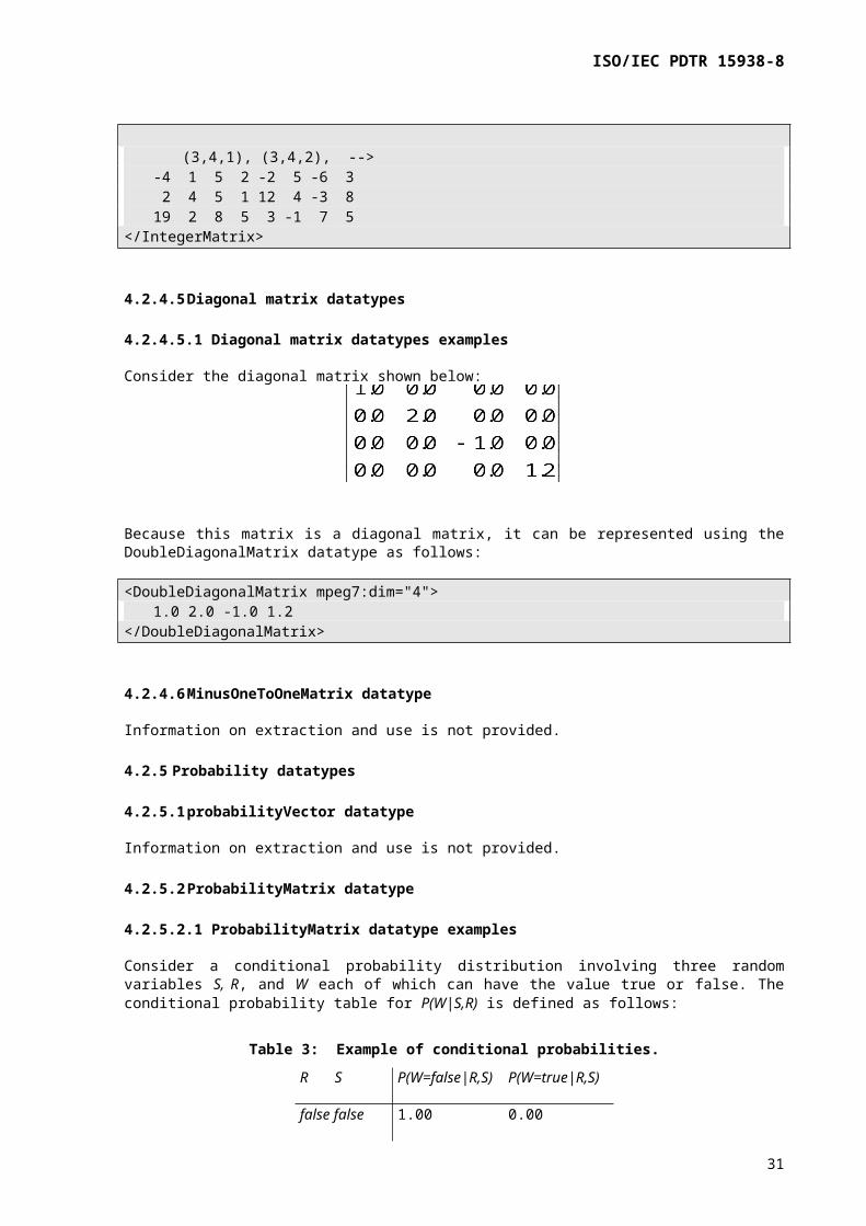
4.2.4.5 Diagonal matrix datatypes
4.2.4.5.1 Diagonal matrix datatypes examples
Consider the diagonal matrix shown below:
Because this matrix is a diagonal matrix, it can be represented using the DoubleDiagonalMatrix datatype as follows:
<DoubleDiagonalMatrix mpeg7:dim="4">1.0 2.0 -1.0 1.2
</DoubleDiagonalMatrix>
4.2.4.6 MinusOneToOneMatrix datatype
Information on extraction and use is not provided.
26

ISO/IEC PDTR 15938-8
4.2.5 Probability datatypes
4.2.5.1 probabilityVector datatype
Information on extraction and use is not provided.
4.2.5.2 ProbabilityMatrix datatype
4.2.5.2.1 ProbabilityMatrix datatype examples
Consider a conditional probability distribution involving three random variables S, R, and W each of which can have the value true or false. The conditional probability table for P(W|S,R) is defined as follows:
Table 3: Example of conditional probabilities.R S P(W=false|R,S) P(W=true|R,S)
false false 1.00 0.00
false true 0.10 0.90
true false 0.80 0.20
true true 0.01 0.99
Then this conditional probability table is represented as a ProbabilityMatrix value as follows. In this example, false is represented as index 1 and true as index 2 and the random variables have been assigned to matrix dimensions as follows: R to dimension 1, S to dimension 2 and W to dimension 3. This results in the following value for ProbabilityMatrix:
<ProbabilityMatrix mpeg7:dim="2 2 2">1.0 0.0 <!-- P(W=false|R=false,S=false), P(W=true|R=false,S=false)
-->0.1 0.9 <!-- P(W=false|R=false,S=true), P(W=true|R=false,S=true)
-->0.8 0.2 <!-- P(W=false|R=true,S=false), P(W=true|R=true,S=false)
-->0.01 0.99 <!-- P(W=false|R=true,S=true), P(W=true|R=true,S=true) -->
</ProbabilityMatrix>
Note that one could have used another assignment of variables to indexes rather than the one used in the example above.
4.2.6 String datatypes
4.2.6.1 mimeType datatype
Information on extraction and use is not provided.
4.2.6.2 countryCode datatype
4.2.6.2.1 countryCode datatype example
The following shows an example of using a countryCode. In this example, the country "Spain" is identified by its code "es".
27

ISO/IEC PDTR 15938-8
<Country>es</Country>
4.2.6.3 regionCode datatype
4.2.6.3.1 regionCode datatype example
The following show examples of encoding places using region codes. Note that region codes are case insensitive.
<Place><Name>Italian province of Milano</Name><Region>IT-MI</Region>
</Place>
<Place><Name>Danish county Roskilde</Name><Region>dk-025</Region>
</Place>
<!-- This example purposely uses mixed case to show case-insensitivity of country/region codes -->
<Place><Name>Antananarivo province in Madagascar</Name><Region>mG-t</Region>
</Place>
4.2.6.4 currencyCode datatype
4.2.6.4.1 currencyCode datatype example
The following shows several examples of different currency codes:
Currency Name Currency Code
Hong Kong Dollar HKD
Euro EUR
4.2.6.5 characterSetCode datatype
4.2.6.5.1 characterSetCode datatype example
The following table shows several examples of character set codes:
Table 4: Examples of character set codes.Character Set Code
Shift JIS encoding of Japanese character
Shift_JIS
28

ISO/IEC PDTR 15938-8
RFC 2279 defined encoding of the ISO/IEC 10646 (Unicode) character set.
UTF-8
29

ISO/IEC PDTR 15938-8
4.3 Linking, identification and localization tools
4.3.1 Introduction
This clause specifies a set of basic datatypes that are used for referencing within descriptions and linking of descriptions to multimedia content. While the DDL already includes a large library of built-in datatypes, the linking to multimedia data requires some additional datatypes, which are defined in this clause:
Table 5: Overview of Linking Tools.Tool Functionality
References to Ds and DSs Tool for representing references to parts of a description. The ReferenceType is defined as a referencing mechanism based on anyURI, IDREF or xPathRefType datatypes.
Unique Identifier Tool for representing unique identifiers of content.
Time description tools Tools for representing time specifications. Two formats are distinguished: the TimeType for time and date specifications according to the real world time and MediaTimeType for time and date specifications as they are used within media.
Media Locators Tools for representing links to multimedia data.
4.3.2 References to Ds and DSs
4.3.2.1 Reference datatype
4.3.2.1.1 Reference datatype examples
The Reference datatype is used in several DSs that rely on the relations between elements of the description. Typical examples include the relation graphs and summarization. See clause 4.8 and clause 4.9 for description examples. Here, examples for the instantiation of the three referencing mechanisms in the ReferenceType are given.
<MyElement href="www.example.com/another-description.mp7#id1">...</MyElement><!-- more elements here --><MyElement idref="id3">...</MyElement><!-- more elements here --><MyElement xpath="../../../MyTargetElement[1]">...</MyElement><!-- more elements here -->
The first example shows a reference to an element with the ID "id1" in "another-description.mp7". The second example references an element with the ID "id3" in the current description. Additionally in the second example the parser checks if there is an attribute of type ID "id3" specified in the current description. In the third example, an XPath expression is used to refer to the first MyTargetElement contained as a child after going up three times in the description tree along the parent axis from the current element which contains the specified XPath attribute.
4.3.2.2 XPath datatypes
Information on extraction and use is not provided.
30
ISO/IEC PDTR 15938-8
4.3.3 Unique Identifier
4.3.3.1 UniqueID datatype
4.3.3.1.1 UniqueID datatype examples
A book can be identified by using the International Standard Book Number (ISBN):
<MyID type="ISBN">0-7803-5610-1</MyID>
An International Standard Work Code (ISWC) can also be specified:
<MyID organization="ISO" type="ISWC">T-034.524.680-1</MyID>
A URN may also be used as a unique identifier as follows: <MyID>urn:ietf:std:50</MyID>
Note that in this case the type and the organization are not specified in the attributes as they are already encoded in the identifier value itself. Furthermore, in this case the type of the identifier (URI) is the default value of "type" and does not need to be specified.
The Unique Identifier datatype can be used when an identification of content is required, either the content or an instance of it. It can also be used as a unique reference to external entities, for example, to identify the rights associated with the content via a rights identifier belonging to an external IPMP system.
4.3.4 Time description tools
4.3.4.1 Time datatype
Information on extraction and use is not provided.
4.3.4.2 TimePoint datatype
Information on extraction and use is not provided.
4.3.4.3 Duration datatype
Information on extraction and use is not provided.
4.3.4.4 IncrDuration datatype
Information on extraction and use is not provided.
4.3.4.5 RelTimePoint datatype
Information on extraction and use is not provided.
4.3.4.6 RelIncrTimePoint datatype
Information on extraction and use is not provided.
4.3.4.7 TimeProperty attribute group
Information on extraction and use is not provided.
31

ISO/IEC PDTR 15938-8
4.3.4.8 Time datatype examples
A Description of an event that started on the 3rd October 1987 at 14:13 in Germany and that has a duration of 10 days can be specified by:
<Time><TimePoint>1987-10-03T14:13+01:00</TimePoint><Duration>P10D</Duration>
</Time>
If one Picture is taken from this event every Day, the time description of the 3rd picture can be specified as follows:
<Time><RelIncrTimePoint timeUnit="P1D"
timeBase="../../../Time[1]">3</RelIncrTimePoint></Time>
This example counts in time units of one Day and refers to the start time of the event as a timeBase (e.g. first time point specification in the description).
The period of five days after the initial event can thus be specified by:
<Time><RelIncrTimePoint timeUnit="P1D"
timeBase="../../../Time[1]">0</RelIncrTimePoint><IncrDuration timeUnit="P1D">5</IncrDuration>
</Time>
An event occurring in England, two hours and 20 minutes after the initial one can be specified by:
<Time><RelTimePoint timeBase="../../../Time[1]">PT2H20M-01:00Z</RelTimePoint>
</Time>
This specification is similar to the example using RelIncrTimePoint. But here the time offset is specified by using a number of hours and minutes instead of counting time units. Additionally it is specified that the time zone is different. Thus the local time is not +01:00 as it was the case for the initial event but +00:00 UTC.
Further examples of time expressions can be found in the clause on MediaTime. The Time datatype can be used whenever there is a need to describe a time segment whether it is a time point or a whole period.
4.3.4.9 MediaTime datatype examples
Consider a video consisting of the following segments:
Segment1: 0-0.1(sec)
Segment2: 0.1-1(sec)
Segment3: 1-10 (sec)
Segment4: 10-20 (sec)
32
ISO/IEC PDTR 15938-8
Segment5: 20-1000 (sec)
The video and these segments are described using the MediaTime datatype in different ways in these examples. Remind that this is done to explain the possibilities of the MediaTime datatype. In a description usually only one of these possibilities are used throughout the document.
Segment 1 is described by using the start time of the video as time base: the XPath expression is applied relative to the context node which is the element in which the mediaTimeBase attribute is contained. For instance "../../MediaLocator[1]" specifies the first MediaLocator contained in the parent node in which also the MediaTime element is contained. Accordingly the time line of the located media element is used to specify the video segment by the start time and the duration of the segment.
<!-- Specification of the video location --><MediaLocator> <MediaUri>http://www.mpeg7.org/the_video.mpg</MediaUri></MediaLocator>
<!-- MediaTime for Segment1(0-0.1sec) --><MediaTime> <MediaRelTimePoint mediaTimeBase="../../MediaLocator[1]">PT0S</MediaRelTimePoint> <MediaDuration>PT1N10F</MediaDuration></MediaTime>
Segment 2 is also specified by the start time of the segment and the duration.
<!-- MediaTime for Segment2(0.1-1sec) --><MediaTime> <MediaRelTimePoint
mediaTimeBase="../../MediaLocator[1]">PT1N10F</MediaRelTimePoint> <MediaDuration>PT9N10F</MediaDuration></MediaTime>
For segment 3 counting mediaTimeUnits are used for the specification of the start time and the duration. The mediaTimeUnit is specified as 1N which is 1/30 of a second according to 30F. But if needed a mediaTimeUnit for the exact sampling rate of NTSC of 29.97...Hz is also possible with: mediaTimeUnit="PT1001N30000F". For the representation of the exact sampling rate of 25Hz in the case of the PAL or SECAM video format the time unit shall be instatiated by mediaTimeUnit="PT1N25F".
<!-- MediaTime for Segment3(1-10sec) --><MediaTime> <MediaRelIncrTimePoint mediaTimeUnit="PT1N30F" mediaTimeBase="../../MediaLocator[1]">30</MediaRelIncrTimePoint> <MediaIncrDuration mediaTimeUnit="PT1N30F">270</MediaIncrDuration></MediaTime>
The last segment again specifies the time using seconds and minutes.
<!-- MediaTime for Segment4(10-20sec) --><MediaTime> <MediaRelIncrTimePoint mediaTimeUnit="PT1N30F" mediaTimeBase="../../MediaLocator[1]">300</MediaRelIncrTimePoint> <MediaIncrDuration mediaTimeUnit="PT1N30F">300</MediaIncrDuration></MediaTime>
33

ISO/IEC PDTR 15938-8
<!-- MediaTime for Segment5(20-1000sec) --><MediaTime> <MediaRelTimePoint mediaTimeBase="../../MediaLocator[1]">PT20S</MediaRelTimePoint> <MediaDuration>PT16M20S</MediaDuration></MediaTime>
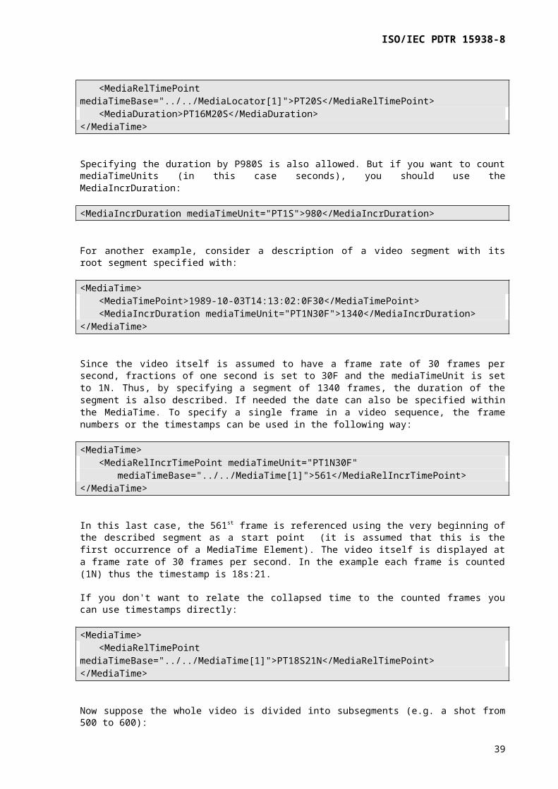
Specifying the duration by P980S is also allowed. But if you want to count mediaTimeUnits (in this case seconds), you should use the MediaIncrDuration:
<MediaIncrDuration mediaTimeUnit="PT1S">980</MediaIncrDuration>
For another example, consider a description of a video segment with its root segment specified with:
<MediaTime><MediaTimePoint>1989-10-03T14:13:02:0F30</MediaTimePoint><MediaIncrDuration mediaTimeUnit="PT1N30F">1340</MediaIncrDuration>
</MediaTime>
Since the video itself is assumed to have a frame rate of 30 frames per second, fractions of one second is set to 30F and the mediaTimeUnit is set to 1N. Thus, by specifying a segment of 1340 frames, the duration of the segment is also described. If needed the date can also be specified within the MediaTime. To specify a single frame in a video sequence, the frame numbers or the timestamps can be used in the following way:
<MediaTime><MediaRelIncrTimePoint mediaTimeUnit="PT1N30F"
mediaTimeBase="../../MediaTime[1]">561</MediaRelIncrTimePoint></MediaTime>
In this last case, the 561st frame is referenced using the very beginning of the described segment as a start point (it is assumed that this is the first occurrence of a MediaTime Element). The video itself is displayed at a frame rate of 30 frames per second. In the example each frame is counted (1N) thus the timestamp is 18s:21.
If you don't want to relate the collapsed time to the counted frames you can use timestamps directly:
<MediaTime><MediaRelTimePoint
mediaTimeBase="../../MediaTime[1]">PT18S21N</MediaRelTimePoint></MediaTime>
Now suppose the whole video is divided into subsegments (e.g. a shot from 500 to 600):
<MediaTime><MediaRelIncrTimePoint mediaTimeUnit="PT1N30F"
mediaTimeBase="../../MediaTime[1]">500</MediaRelIncrTimePoint><MediaIncrDuration mediaTimeUnit="PT1N30F">100</MediaIncrDuration>
</MediaTime>
and you want to address within this segment the above-mentioned frame:
<MediaTime>
34

ISO/IEC PDTR 15938-8
<MediaRelIncrTimePoint mediaTimeUnit="PT1N30F" mediaTimeBase="../../../MediaTime">61</MediaRelIncrTimePoint></MediaTime>
In this case the start time of the shot (e.g. the parent node of the node which contains the present MediaTime datatype) is referenced as mediaTimeBase.
To avoid to specify repeatedly the mediaTimeUnit and the mediaTimeBase in the media time specification the mediaTimeUnit and mediaTimeBase attribute can be used in a DS:
<VideoSegment mediaTimeUnit="PT1N30F" mediaTimeBase="MediaLocator"><!-- more elements here -->
</VideoSegment>
If the specified mediaTimeUnit and mediaTimeBase attributes are instantiated in an ancestor of this media time specification the above mentioned frame can be addressed by
<MediaTime><MediaRelIncrTimePoint>61</MediaRelIncrTimePoint>
</MediaTime>
The datatype can be used whenever there is a need to specify a time segment whether it is a time point or a whole period using the time information of the AV content. For example the MediaTime datatype is used within the MediaLocator datatype.
4.3.5 Media Locators
4.3.5.1 MediaLocator datatype
4.3.5.2 InlineMedia datatype
4.3.5.2.1 InlineMedia datatype examples
The InlineMedia datatype enables for instance an embedding of small audio clips and image thumbnails in the description, without having to refer to external data. An example is as follows.
<!-- <element name="MyInlineMedia" type="mpeg7:InlineMediaType"/> -->
<MyInlineMedia type="image/jpeg"><MediaData16>98A34F10C5094538AB9387362522DA3</MediaData16>
</MyInlineMedia>
4.3.5.3 TemporalSegmentLocator datatype
Information on extraction and use is not provided.
4.3.5.4 ImageLocator datatype
Information on extraction and use is not provided.
35

ISO/IEC PDTR 15938-8
4.3.5.5 MediaLocator datatype examples
<MyTemporalSegmentLocator><MediaUri>http://www.mpeg7.org/demo.mpg</MediaUri><MediaTime>
<MediaRelTimePoint mediaTimeBase="../../MediaUri">PT3S</MediaRelTimePoint>
<MediaDuration>PT10S</MediaDuration></MediaTime>
</MyTemporalSegmentLocator>
<MyMediaLocator><MediaUri>http://www.mpeg7.org/demo.mp4</MediaUri><StreamID>1</StreamID>
</MyMediaLocator>
<MyImageLocator><MediaUri>http://www.mpeg7.org/demo.ppm</MediaUri><BytePosition offset="1024"/>
</MyImageLocator>
In the first example the location of a video segment is specified by the URI of a video file and the relative start time with respect to the beginning of the file and the duration of the segment. In the second example, the MediaLocator refers to a particular stream within an MPEG-4 file. In the third example, the media data is simply located using a byte-offset from the start of a known file.
36

ISO/IEC PDTR 15938-8
4.4 Basic description tools
4.4.1 Introduction
This clause defines the basic tools, which are used as components for building other description tools. The basic tools are used in this part of the standard (ISO/IEC 15039-5) and also in audio part (see ISO/IEC 15938-4) and visual (see ISO/IEC 15938-3) part. The tools defined in this clause are as follows.
Table 6: Overview of Basic Description Tools.Tool Functionality
Language Identification Tools for identifying the language of a textual description or of the multimedia content itself. This standard uses the XML defined xml:lang attribute to identify the language used to write a textual description.
Text Annotation Tools for representing unstructured and structured textual annotations. Unstructured annotations (i.e. with free text) are represented using the FreeTextAnnotation datatype. Annotations that are structured in terms of answering the questions "Who? What? Where? How? Why?" are represented using the StructuredAnnotation datatype. Annotations structured as a set of keywords are representations using the KeywordAnnotation datatype. Finally, annotations structured by syntactic dependency relations—for example, the relation between a verb phrase and its subject—are represented using the DependencyStructure datatype.
Classification Schemes and Terms
Tools for classifying using language-independent terms and for defining sets of terms as classification schemes. The ClassificationScheme DS describes a vocabulary for classifying a subject area as a set of terms organized into a hierarchy. A term defined in a classification scheme is used in a description with the TermUse or ControlledTermUse datatypes.
Graphical classification schemes are schemes for classifying where the terms in the scheme are themselves graphs. Such schemes can be used as structural templates, for validating of graph-based descriptions, and for graph productions.
Agents Tools for describing "agents", including persons, groups of persons, and organizations. The Person DS represents a person, the PersonGroup DS a group of persons, and the Organization DS an organization of people.
Places Tools for describing geographical locations. The Place DS is used to describe real and fictional places.
Graphs and Relations Tools for representing relations and graph structures. The Relation DS is a tool for representing named relations between instances of description tools. The Graph DS organizes relations into a graph structure.
Ordering The OrderingKey DS describes hints for ordering descriptions
Affective Description The Affective DS describes an audience's affective response to
37

ISO/IEC PDTR 15938-8
multimedia content.
Phonetic Description The PhoneticTranscriptionLexicon DS describes the pronunciations of a set of words.
4.4.2 Language identification
4.4.2.1 xml:lang attribute
4.4.2.1.1 xml:lang attribute examples
Consider the following example:
<TextAnnotation xml:lang="en"><KeywordAnnotation>
<Keyword xml:lang="fr"> chien </Keyword><Keyword> dog </Keyword>
</KeywordAnnotation></TextAnnotation>
In this example, the outer level TextAnnotation specifies that the language of the description is English ("en"). This automatically applies to all elements contained and thus the value of the xml:lang for the contained Keyword "dog", defaults to be English. However, because the keyword "chien" specifies that the language is French ("fr") using xml:lang, this value overrides the language specified in the containing TextAnnotation.
4.4.2.2 language datatype
4.4.2.2.1 language datatype examples
The xsd:language datatype is used for identifying the language properties of the multimedia content. For example, to indicate the language used in the audio, the written language of subtitles, or a user's preferred language for viewing content.
The example below states that the preferred language is English.
<PreferredLanguage>en</PreferredLanguage>
4.4.3 Textual annotation
4.4.3.1 Textual datatypes
4.4.3.1.1 Textual datatypes example
For examples of the use of these datatypes, see the subclause specifying the TextAnnotation datatype.
38

ISO/IEC PDTR 15938-8
4.4.3.2 TextAnnotation datatype
4.4.3.2.1 TextAnnotation datatype examples
The following example shows an annotation of a video depicting the scene "Tanaka throws a small ball to Yamada. Yamada catches the ball with his left hand."
<Mpeg7><Description xsi:type="ContentEntityType">
<MultimediaContent xsi:type="VideoType"><Video>
<MediaLocator><MediaUri>video.mpg</MediaUri>
</MediaLocator><TextAnnotation>
<FreeTextAnnotation xml:lang="en">Tanaka throws a small ball to Yamada.Yamada catches the ball with his left hand.
</FreeTextAnnotation><StructuredAnnotation>
<Who href="urn:people:TANAKA100"><Name xml:lang="en">Tanaka</Name>
</Who><Who>
<Name xml:lang="en"> Yamada </Name></Who><WhatObject>
<Name xml:lang="en"> A small ball </Name></WhatObject><WhatAction>
<Name xml:lang="en"> Tanaka throws a small ball to Yamada.
</Name></WhatAction><WhatAction>
<Name xml:lang="en"> Yamada catches the ball with his left
hand. </Name></WhatAction>
</StructuredAnnotation></TextAnnotation>
</Video></MultimediaContent>
</Description></Mpeg7>
In this example, there are two different forms of the annotation for the same event:
Free text annotation. This is simply an English description of what happened in the scene without any structuring.
Structured text annotation. In this case the annotation is more structured; "Yamada" is identified as the "Who" and the ball he is throwing as the "What" in the annotation. Also, notice that Yamada is identified using a term "urn:people:TANAKA100" from a classification scheme for identifying people (identified as "urn:people"). .
4.4.3.3 StructuredAnnotation datatype
Information on extraction and use is not provided.
39

ISO/IEC PDTR 15938-8
4.4.3.4 KeywordAnnotation datatype
4.4.3.4.1 KeywordAnnotation datatype examples
The following example shows an annotation describing a video about the U.S. presidential election using keywords:
<Mpeg7><Description xsi:type="ContentEntityType">
<MultimediaContent xsi:type="VideoType"><Video>
<TextAnnotation><KeywordAnnotation xml:lang="en">
<Keyword>election</Keyword><Keyword>United States of America</Keyword><Keyword>President</Keyword>
</KeywordAnnotation></TextAnnotation>
</Video></MultimediaContent>
</Description></Mpeg7>
4.4.3.5 DependencyStructure datatype
4.4.3.5.1 DependencyStructure datatype examples
The following rules specify the dependency relations in English:
Governor Dependent Operator/FunctionWord(of DependencyStructure datatype)
Example(G: Governor, D: Dependent)
Verb Noun subject John (D) drank (G)
Verb Noun object drink (G) water (D)
Verb Noun indirectObject tell (G) you (D) the fact
Verb Preposition functionWord=(Preposition) respect (G) for (D) Johnsit (G) on (D) a chair
VerbNounAdjectivePreposition
predicate
make (G) it possible (D)are (G) friends (D)is (G) without (D) a hatJohn returned (G) rich (D)
Verb Adverb walk (G) fast (D)
Verb Conjunction functionWord=(Conjunction) started (G) before (D) I finished breakfast
Noun Adjective good (D) friends (G)
Noun Genitive John’s (D) friends (G)
Noun Determiner the (D) cake (G)
Noun Noun London (D) hospital (G)
40
ISO/IEC PDTR 15938-8
Governor Dependent Operator/FunctionWord(of DependencyStructure datatype)
Example(G: Governor, D: Dependent)
Noun Preposition functionWord=(Preposition) years (G) of (D) war
Noun VerbfunctionWord=(Relative-pronoun) people (G) who think (D) that
Adjective Adverb very (D) good (G)
Preposition Noun in (G) water (D)
Conjunction Verb before (G) I finished (D) breakfast
Auxiliary verb Verb can (G) read (D) a book
"to“ Verb to (G) go (D) to bed
Rules for other languages can be specified in a similar fashion but are not specified by this standard.
Consider the dependency structure of the following sentence: "John talks to Mary whom he loves." According the rule above, the following tree structure (syntactic tree) represents the dependency structure of the sentence.
Figure 1: Example of dependency structure of the sentence: "John talks to Mary whom he loves.“
The solid arrows in Figure 1 show dependency relations and the dashed arrows indicate coreference relations. The labels attached to the arrows indicate the type of dependency relation. Specifically, the verb "talks" governs "John" and "to (Mary)", while "Mary" governs a verb "loves“ in a relative clause. In the relative clause, the verb "loves" governs "whom", which refers "Mary“ in a main clause, and "he", which refers to "John“.
The following shows the example represented using the DependencyStructure datatype:
<Mpeg7><Description xsi:type="ContentEntityType">
<MultimediaContent xsi:type="VideoType">
John to
whom he
talks
subject “to”
loves
subjectobject
Mary“whom”
41

ISO/IEC PDTR 15938-8
<Video><TextAnnotation>
<DependencyStructure xml:lang="en"><Sentence>
<Phrase operator="subject"><Head type="noun" id="JOHN">John</Head>
</Phrase><Head type="verb" baseForm="talk">talks</Head><Phrase functionWord="to">
<Head type="preposition">to</Head><Phrase>
<Head type="noun" id="MARY">Mary</Head><Phrase functionWord="whom">
<Phrase operator="object"><Head type="pronoun"
equal="MARY">whom</Head></Phrase><Phrase operator="subject">
<Head type="pronoun" equal="JOHN">he</Head>
</Phrase><Head type="verb"
baseForm="love">loves</Head></Phrase>
</Phrase></Phrase>
</Sentence></DependencyStructure>
</TextAnnotation></Video>
</MultimediaContent></Description>
</Mpeg7>
Notice that the preposition "to" is represented as a functionWord attribute attached to the Phrase element representing "to Mary who he loves".
4.4.3.5.2 DependencyStructure datatype extraction
Using a natural language parser (NL parser), it is possible to generate the dependency structure for manually generated free text annotations. For example, one can automatically extract the following information:
Dependency structures
Syntactic role of phrases in the annotation-sentences (relationship with governor is represented by the particle attribute and the operator attribute).
In general, natural language syntactic analysis involves some ambiguity, i.e., a unique solution cannot always be given. The constrained annotations generated by professionals have a relatively simple structure and high accuracy can generally be obtained. On the other hand, amateur annotations, which tend to include many modifiers that make sentences long, results in relatively low analysis accuracy.
Human correction for erroneous results of the syntactic analysis is usually needed. Most of the errors come from the syntactic ambiguity about which phrase modifies which term. Correcting this type of error needs semantic analysis of the sentences. But the error can be fixed by simply changing a governor term (i.e., head) of a modifier phrase (i.e., dependent), which is not very complicated for humans. The syntactic analysis by the NL parser is helpful for instantiation of the Dependency
42

ISO/IEC PDTR 15938-8
Structure not only from the professional style annotations but also from the amateur style ones that include syntactic ambiguity.
One can retrieve audio or video segments using natural language as an interface by describing video segment with the DependencyStructure datatype. To do this a video segment index is prepared according to the following procedure.
For each segment, the syntactic tree representing an instance of the Dependency Structure is converted to a tree structure for index use. In the tree structure, a noun that is a head of a "sentence" or a head of a phrase that depends on a predicate of a "sentence" as a subject is taken to be the root node. If no such term exists, a dummy node is added.
ball foot
subject object “with”
Tree of Dependency Structure Tree for Index(Subject-centered
Dependency Structure)
kick
ball
kick
foot
“with”object
Tom
Tom
verb verb
subject
All tree structures for the segment index included in the database are merged to form a database index tree.
kickobject
ball field
run
“towards”
goal
subjectJohn
kick
ball
object
subjectShot#1 “Tom kicks a ball”Shot#2 “John”Shot#3 “Tom runs towards the goal”Shot#4 “John kicks a ball”Shot#5 “Tom kicks the field”
Shot#1
Shot#2
Shot#3Shot#4 Shot#5
Tomsubject
object
Each node in the index tree stores a pointer to the segment in question. Therefore, to perform a search using this index tree, a natural language search query is first converted to a tree structure. This tree is then matched with the index trees to find the desired segment.
Matching may be achieved by partial tree matching and, in the case of inter-node matching, similarity-based retrieval can be performed by using a thesaurus or the like. The reason for configuring an index tree centered about the subject/theme is that candidate can be narrowed down from the start through the use of subjects/themes, which provide the most information in keyword-centered annotations.
An example system is configured as follows.
43

ISO/IEC PDTR 15938-8
DependencyStructure
Description (Well-formed XML Document)
XML parser(DOM API)
Index Generator
Index
Query (in Natural Language) NL parser
Tree Representationfor Matching
Matching Results
DS for a videosegment
Traditionally, keywords are used when retrieving based on language. However, using the Dependency Structure has the following advantages.
It supports retrieval that specify inter-element relationships such as "A gives B to C" which cannot be expressed solely by Boolean operators (AND/OR) as employed in ordinary keyword retrieval.
It supports flexible retrieval by allowing the use of "wild cards" such as in the expression "C eats something."
It requires no special query language (retrieval can be performed with natural language sentences).
4.4.4 Classification Schemes and Terms
4.4.4.1 ClassificationScheme DS
4.4.4.1.1 ClassificationScheme format and importing
Information on extraction and use is not provided.
4.4.4.1.2 ClassificationScheme DS examples
The following subclauses show several different examples of defining classification schemes.
Classification Scheme Example One: Audio Domain
The following example shows a classification scheme for audio domain. Note that while this example is based on the the AudioDomainCS classification specified in Annex A, it has been modified and simplified here for explanatory purposes. The instance of the ClassificationScheme DS defining the scheme looks as follows:
<Mpeg7><Description xsi:type="ClassificationSchemeDescriptionType">
<ClassificationScheme uri="urn:mpeg:mpeg7:cs:AudioDomainCS"
domain="//MediaInformation/MediaProfile/MediaIdentification/AudioDomain"><Header xsi:type="DescriptionMetadataType">
<Version>1.0</Version>
44

ISO/IEC PDTR 15938-8
<Rights><RightsID>urn:rights:x0d01d</RightsID>
</Rights></Header><Term termID="1">
<Name xml:lang="en">Source</Name><Definition xml:lang="en">Type of audio source</Definition><Term termID="1.1">
<Name xml:lang="en">Synthetic</Name></Term><Term termID="1.2">
<Name xml:lang="en">Natural</Name></Term>
</Term><Term termID="2">
<Name xml:lang="en">Acquisition</Name><Definition xml:lang="en">Type of Content</Definition><Term termID="2.1">
<Name xml:lang="en">Music</Name></Term><Term termID="2.2">
<Name xml:lang="en">Speech</Name><Name xml:lang="jp">Onsei</Name>
</Term><Term termID="2.3">
<Name xml:lang="en">Mixed</Name></Term><Term termID="2.4">
<Name xml:lang="en">Multi-track</Name></Term>
</Term><Term termID="3">
<Name xml:lang="en">Use</Name><Definition xml:lang="en">Original usage domain</Definition><Term termID="3.1">
<Name xml:lang="en">Scientific</Name></Term><Term termID="3.2">
<Name xml:lang="en">Medical</Name></Term><Term termID="3.3">
<Name xml:lang="en">Security</Name></Term><Term termID="3.4">
<Name xml:lang="en">Broadcast</Name></Term><Term termID="3.4">
<Name xml:lang="en">CD-A distribution</Name></Term>
</Term></ClassificationScheme>
</Description></Mpeg7>
The first part of the ClassificationScheme instance contains "header“ information including:
URI. The unique identifier for this ClassificationScheme is a URN: "urn:mpeg:mpeg7:cs:AudioDomainCS“. The first part of the URI "urn:“ indicates that this URI is a URN. In fact, all classification schemes defined in this document use URNs as their unique identifier. The second part of the URN, "mpeg“, is the namespace
45

ISO/IEC PDTR 15938-8
identifier. In this case the namespace identifier ("mpeg“) is one that is registered as belonging to MPEG. Following the "mpeg“ namespace identifier is the namespace specific string "mpeg7", which identifies the classification schemes as being defined in this standard and a "cs" string, which indicates that name, is for a classification scheme. Finally, the "AudioDomainCS“ is the name assigned to the classification scheme within the "mpeg“ URN namespace.
Domain. The suggested domain for this ClassificationScheme is "MediaInformation/MediaProfile/MediaIdentification/AudioDomain“. The domain is expressed as an XPath value. In this case, the XPath matches the AudioDomain element defined inside of the MediaIdentification DS (contained within the MediaProfile DS in the MediaInformation DS).
Description Metadata. This element contains metadata about the ClassificationScheme itself. In the example, the description metadata indicates that this is version "1.0“ of the classification scheme and that the intellectual property rights for the classification scheme are identified by "urn:rights:x0d01d“.
The next part of this ClassificationScheme contains a list of term definitions. This list includes:
Term Identifiers. In this classification scheme, the term identifiers are numerals that encode the term hierarchy. However, this use is simply a convention adopted in this classification scheme. In fact, term identifiers are simply opaque values whose only requirement is that they be unique within the classification scheme. For example, instead of the term identifier "1“ for the term "Source“, the term identiifer might equally well have been "0d3d“ or "source“.
Term Names. Each term in this classification scheme has an English name (the language is indicated by the xml:lang attribute having a value of "en“). The term names are human readable labels for the terms. Note that terms may have names in multiple languages. For example, term "2.2“ has a name in both English ("Speech“) and Japanese ("Onsei“).
Term Definitions. Only terms "1“ and "2“ have prose definitions in this classification scheme. The other terms do not have written definitions, which is allowed because the Definition element in a term is optional.
Term Relations. This classification scheme contains a hierarchy of terms. In others words, it defines broader term/narrower term relations between pairs of terms. For example, term "1“ is a broader term than term "1.1“ and term "1.1“ is a narrower term than term "1“ – these are inverse relations. Note that the definition of term "1.1“ is syntactically contained within the definition of term "1“. This is how term relations are written in a ClassificationScheme. In fact, other kinds of relations can be specified by using the "relation“ attribute to relate the parent and contained terms. Because the default value of a term relation is "NT“, indicating that the contained term is narrower than the containing term.
Classification Scheme Example Two: Genre
The following figure shows an example of a simple classification for genre identified by the URI "urn:example:Genre". In the figure below, round boxes represent classification schemes and square boxes represent terms.
46

ISO/IEC PDTR 15938-8
Figure 2: Illustration of the "Escort2_4:Genre" Genre Classification Scheme.In this example, there are three terms at the highest level: information, drama, and music. Below the category "information", there is a more detailed term: "Sport". Rather than defining a complete classification for sports, this example shows how an existing classification scheme can be imported. The existing "IOC Sport" classification scheme is added below the "Sport" item. Similarly, the drama category imports the "TVE Drama" classification scheme. For music, the sub-terms (narrower in meaning than their containing term) are "Pop", "Rock", "Jazz", and "Classical".
<Mpeg7><Description xsi:type="ClassificationSchemeDescriptionType">
<ClassificationScheme uri="urn:example:Genre" domain="//CreationInformation/Classification/Genre"><Import href="http://www.tvid.org/TVE/Drama/"/><Import href="http://www.ioc.org/IOC/Sports/"/><Term termID="information">
<Name xml:lang="en">Information</Name><Definition xml:lang="en">Generic news</Definition><!-- This narrower term comes from the imported IOC Sports
scheme --><Term termID="sports"/>
</Term><Term termID="drama">
<!-- This narrower term comes from the imported drama scheme-->
</Term><Term termID="music">
<Term termID="rock"><Name xml:lang="en">Rock</Name>
</Term><Term termID="pop">
<Name xml:lang="en">Pop</Name></Term><Term termID="jazz">
<Name xml:lang="en">Jazz</Name></Term><Term termID="classical">
<Name xml:lang="en">Classical</Name></Term>
</Term></ClassificationScheme>
</Description></Mpeg7>
47
ISO/IEC PDTR 15938-8
4.4.4.2 TermDefinition DS
Information on extraction and use is not provided.
4.4.4.3 TermUse datatype
4.4.4.3.1 TermUse datatype examples
4.4.4.3.1.1 Term reference use
The following example shows some examples of term reference using several different means to refer to terms:
<!-- Referring to a term using a URN --><TermUse href="urn:mpeg:mpeg7:cs:GenreCS:alternativeJazz"/>
<!-- Referring to a term using a HTTP URI --><TermUse href="http:://www.mpeg.org/GenreCS.xml#alternativeJazz"/>
<!-- Referring to a term using a classification scheme alias --><!-- Define schema aliases --><ClassifiationSchemeAlias alias="s1" href="urn:mpeg:mpeg7:cs:GenreCS"/><ClassifiationSchemeAlias alias="s2" href="http:://www.mpeg.org/GenreCS.xml"/>
<!-- Refer to the term using the two schema aliases --><TermUse href=":s1:alternativeJazz"/><TermUse href=":s2:alternativeJazz"/>
The reference to the term is included in the href attribute. In the first example, this is the URN "urn:mpeg:mpeg7:cs:GenreCS:alternativeJazz“. Using URN’s to reference terms defined in classification schemes is preferred in general and shall be used for referring to terms defined in this document. However, terms defined in existing classification managed by other organizations can be referred to using any valid URI. For example, the reference "http:://www.mpeg.org/GenreCS.xml#alternativeJazz“ uses a HTTP format for referring to a term. The final two example of TermUse show the use of classification schemes aliases, which provide an abbreviated syntax for referring to terms. In this case, aliases "s1“ is assigned to the classification scheme identified by "urn:mpeg:mpeg7:cs:GenreCS“ and the alias "s2“ is assigned to the classification at "http://www.mpeg.org/GenreCS.xml“. For further details on term references, see the specification of the termReference datatype.
4.4.4.3.1.2 Inline term use
This next example shows an inline term use.
<TermUse href="urn:AISF:Sports:1.4.9"><Name xml:lang="en">Basketball</Name><Definition xml:lang="en">Basket Description</Definition><Term relation="BT" termID="1.4">
<Name xml:lang="en">Sport</Name><Definition xml:lang="en">Sports news</Definition>
<Term relation="BT" termID="1"> <Name xml:lang="en">Information</Name>
<Definition xml:lang="en">Generic news</Definition></Term>
</Term>
48
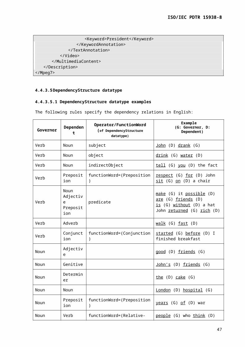
ISO/IEC PDTR 15938-8
</TermUse>
In this example, the term "1.4.9" (i.e. basketball) is taken from the "urn:GAISF:Sports" classification scheme. In addition to the term identifier in the href attribute, the TermUse also includes inline information about the term: its name, definition, and some related terms. In this example, the term "1.4.9“ is related to the broader term "1.4", which is in turn related to the broader term "1". In other words, this indicates that the hierarchy of terms for the genre is: 1.4.9 (Basketball) --> Sports (1.4) --> 1 (Information) .
4.4.4.3.1.3 Free term use
The last example shows the use of TermUse datatype as a free term use.
<TermUse><Name>My genre</Name>
</TermUse>
What distinguishes a free term from a reference TermUse or an inline TermUse is that there is no reference to a term in a classification scheme. Instead of referencing the term, a free term use includes an arbitrary textual name or definition. This use is supported to allow the option of either writing free text or using a term inside of a description. It provides the greatest freedom of expression as no restrictions are imposed. On the other hand, this means that an application may find it difficult to interpret the content of a free TermUse.
4.4.4.4 ControlledTermUse datatype
4.4.4.4.1 ControlledTermUse datatype examples
The following example shows how a ControlledTermUse can refer to a term in an existing classification scheme, which has not been defined as an instance of the ClassificationScheme DS. The first example is taken from The Art and Architecture Thesaurus (AAT) compiled by the Getty Research Institutes. The AAT is a thesaurus widely used for cataloguing in the museum community. This case shows how the term for "High Baroque" in the AAT can be referenced as a controlled term:
<ControlledTermUse href="http://www.getty.edu/aat/21150"><Name xml:lang="en">High Baroque</Name><Definition>The fully Baroque style that emerged in ...</Definition>
</ControlledTermUse>
Note several things about this example:
Term Reference. In this example, the resource for the term is identified by a URI. In the example, the URI identifies the source (the Getty Research Institute) and the term’s identifier ("21150") within the AAT. In the AAT, term identifiers are opaque numeric values.
Name and Definition. Names and definitions can be given for terms in a classification schemes by including them inline inside of the ControlledTermUse. In this case the name indicates that the term means "High Baroque" in English and gives a definition of that term in English (abbreviated in the example).
The second example of referencing a term in an existing classification scheme uses a term in the Dewey Decimal classification scheme (used in many libraries for cataloguing books).
<ControlledTermUse href="urn:dewey:630"><Name xml:lang="en">Agriculture</Name>
</ControlledTermUse>
49

ISO/IEC PDTR 15938-8
50

ISO/IEC PDTR 15938-8
The term is referenced using a URN (made up for the purpose of this example), which indicates that the term comes from the "dewey“ URN identifier space. The "630“ following the colon further qualifies the in the "dewey“ URN space. In this case it indicates that it refers to the "630"; that is, pertaining to agriculture.
4.4.4.5 termReference datatype
4.4.4.5.1 Format of URN for terms
The following defines the normative form of URN for referring to terms defined in classification schemes specified in this or other parts of the ISO/IEC 15938 standard.
If the termReferenceType is a URI, and the term being referenced is defined in ISO/IEC 15938, whether normative or informative, then the URI shall be a URN of the following form:
urn:mpeg:mpeg7:cs:SchemeName:termID"
The "urn:mpeg:mpeg7:cs:SchemeName“ is the URN identifying the classification scheme for this term, as specified in 4.4.4. The termID part of the URN shall match the termID attribute value specified for the term in the term's definition. Note however that URN's defined in the MPEG URN namespace are case insensitive and therefore the use of upper and lowercase letters are not distinguished in both termID and schemeName
For classification schemes that are not defined in ISO/IEC 15938, the form of the URI used to reference terms is not specified by this standard. However, using a URN for term reference URIs is strongly recommended.
4.4.4.6 ClassificationSchemeAlias datatype
Information on extraction and use is not provided.
4.4.4.7 GraphicalClassificationScheme DS
Information on extraction and use is not provided.
4.4.4.8 GraphicalTermDefinition DS
Information on extraction and use is not provided.
4.4.4.9 GraphicalRuleDefinition DS
Information on extraction and use is not provided.
4.4.4.10 PullbackDefinition DS
Information on extraction and use is not provided.
4.4.4.11 DoublePullbackDefinition DS
Information on extraction and use is not provided.
4.4.4.12 PushoutDefinition DS
Information on extraction and use is not provided.
51

ISO/IEC PDTR 15938-8
4.4.4.13 DoublePushoutDefinition DS
Information on extraction and use is not provided.
4.4.4.14 GraphicalTermDefinition DS examples
The complete example description follows:
<Mpeg7><Description xsi:type="ClassificationSchemeDescriptionType">
<ClassificationSchemeBase xsi:type="GraphicalClassificationSchemeType"
uri="urn:example:cs:Graph1"><GraphicalTerm termID="1">
<AlphabetGraph id="ag"><Node id="unknown">
<Name href="urn:example:any"/></Node><Node id="boundary">
<Name href="urn:example:Object"/></Node><Node id="context">
<Name href="urn:example:any"/></Node><Relation id="ag1" source="#unknown" target="#unknown"
type="urn:example:any"/><Relation id="ag2" source="#boundary" target="#unknown"
type="urn:example:any"/><Relation id="ag3" source="#unknown" target="#boundary"
type="urn:example:any"/><Relation id="ag4" source="#boundary" target="#context"
type="urn:example:any"/><Relation id="ag5" source="#context" target="#boundary"
type="urn:example:any"/><Relation id="ag6" source="#context" target="#context"
type="urn:example:any"/></AlphabetGraph>
</GraphicalTerm><GraphicalTerm termID="2">
<ProductionRule xsi:type="PullbackDefinitionType"><RuleGraph id="rg">
<Node id="rghand"><Name href="urn:example:HandObject"/>
</Node><Node id="rgboundary">
<Name href="urn:example:Object"/></Node><Node id="rgcontext">
<Name href="urn:example:any"/></Node><Relation id="rg1" source="#rgboundary"
target="#rghand" type="urn:example:contains"/>
<Relation id="rg2" source="#rgboundary" target="#rgcontext"
type="urn:example:any"/><Relation id="rg3" source="#rgcontext"
target="#rgboundary" type="urn:example:any"/>
<Relation id="rg4" source="#rgcontext" target="#rgcontext"
52

ISO/IEC PDTR 15938-8
type="urn:example:any"/></RuleGraph><AlphabetGraphRef href="urn:example:cs:Graph1:1"/><MorphismGraph>
<Relation source="#rghand" target="#unknown"
type="urn:mpeg:mpeg7:cs:GraphRelationCS:2001:identity"/><Relation source="#rgboundary" target="#boundary"
type="urn:example:any"/><Relation source="#rgcontext" target="#context"
type="urn:example:any"/><Relation source="#rg1" target="#ag2"
type="urn:example:any"/><Relation source="#rg2" target="#ag4"
type="urn:example:any"/><Relation source="#rg3" target="#ag5"
type="urn:example:any"/><Relation source="#rg4" target="#ag6"
type="urn:example:any"/><SourceGraphRef href="#rg"/><TargetGraphTermRef href="urn:example:cs:Graph1:1"/>
</MorphismGraph></ProductionRule>
</GraphicalTerm></ClassificationSchemeBase>
</Description><Description xsi:type="SemanticDescriptionType">
<Semantics><Label>
<Name>Semantic description of "person" with "leftarm" and "rightarm".
</Name></Label><SemanticBase xsi:type="ObjectType" id="person">
<Label><Name>Person</Name>
</Label></SemanticBase><SemanticBase xsi:type="ObjectType" id="leftarm">
<Label><Name>left arm</Name>
</Label></SemanticBase><SemanticBase xsi:type="ObjectType" id="rightarm">
<Label><Name>right arm</Name>
</Label></SemanticBase><Graph id="persongraph">
<Relation id="person1" type="urn:example:has" source="#person" target="#leftarm"/>
<Relation id="person2" type="urn:example:has" source="#person" target="#rightarm"/>
</Graph></Semantics>
</Description><Description xsi:type="SemanticDescriptionType">
<Semantics><Label>
<Name> Morphisms graph of relations </Name></Label>
53

ISO/IEC PDTR 15938-8
<Graph xsi:type="MorphismGraphType"><Relation source="#object3" target="#tom1"
type="urn:mpeg:mpeg7:cs:GraphRelationCS:2001:identity"/><Relation source="#object4" target="#mary1"
type="urn:mpeg:mpeg7:cs:GraphRelationCS:2001:identity"/><Relation source="#lhs1" target="#ew1"
type="urn:mpeg:mpeg7:cs:GraphRelationCS:2001:identity"/><SourceGraphTermRef href="urn:example:cs:Graph2:1"/><TargetGraphRef href="#eastwestgraph"/>
</Graph></Semantics>
</Description></Mpeg7>
<Mpeg7><Description xsi:type="ClassificationSchemeDescriptionType">
<ClassificationSchemeBase xsi:type="GraphicalClassificationSchemeType"
uri="urn:example:cs:Graph2"><GraphicalTerm termID="1">
<AlphabetGraph id="ag"><Node id="unknown">
<Name href="urn:example:any"/></Node><Node id="context">
<Name href="urn:example:any"/></Node><Relation id="ag1" source="#unknown" target="#unknown"
type="urn:example:any"/><Relation id="ag2" source="#unknown" target="#context"
type="urn:example:any"/><Relation id="ag3" source="#context" target="#unknown"
type="urn:example:any"/><Relation id="ag4" source="#context" target="#context"
type="urn:example:any"/></AlphabetGraph>
</GraphicalTerm><GraphicalTerm termID="2">
<ProductionRule xsi:type="DoublePullbackDefinitionType"><RuleGraph id="rule1">
<Node id="rg1context"><Name href="urn:example:any"/>
</Node><Node id="sun">
<Name href="urn:example:Sun"/></Node><Node id="waves">
<Name href="urn:example:waves"/></Node><Node id="fish">
<Name href="urn:example:fish"/></Node><Relation id="rg11" source="#rg1context"
target="#context" type="urn:example:any"/>
<Relation id="rg12" source="#rg1context" target="#sun" type="urn:example:contains"/>
54

ISO/IEC PDTR 15938-8
<Relation id="rg13" source="#rg1context" target="#waves"
type="urn:example:contains"/><Relation id="rg14" source="#rg1context" target="#fish"
type="urn:example:contains"/></RuleGraph><RuleGraph id="rule2">
<Node id="rg2context"><Name href="urn:example:any"/>
</Node><Node id="clouds">
<Name href="urn:example:clouds"/></Node><Node id="icebergs">
<Name href="urn:example:icebergs"/></Node><Node id="seals">
<Name href="urn:example:seals"/></Node><Relation id="rg21" source="#rg2context"
target="#context" type="urn:example:any"/>
<Relation id="rg22" source="#rg2context" target="#clouds"
type="urn:example:contains"/><Relation id="rg23" source="#rg2context"
target="#icebergs" type="urn:example:contains"/>
<Relation id="rg24" source="#rg2context" target="#seals"
type="urn:example:contains"/></RuleGraph><AlphabetGraphRef href="urn:example:cs:Graph2:1"/><MorphismGraph>
<Relation source="#rg1context" target="#context"
type="urn:mpeg:mpeg7:cs:GraphRelationCS:2001:identity"/><Relation source="#waves" target="#unknown"
type="urn:mpeg:mpeg7:cs:GraphRelationCS:2001:identity"/><Relation source="#sun" target="#unknown"
type="urn:mpeg:mpeg7:cs:GraphRelationCS:2001:identity"/><Relation source="#fish" target="#unknown"
type="urn:mpeg:mpeg7:cs:GraphRelationCS:2001:identity"/><Relation source="#rg11" target="#ag4"
type="urn:mpeg:mpeg7:cs:GraphRelationCS:2001:identity"/><Relation source="#rg12" target="#ag3"
type="urn:mpeg:mpeg7:cs:GraphRelationCS:2001:identity"/><Relation source="#rg13" target="#ag3"
type="urn:mpeg:mpeg7:cs:GraphRelationCS:2001:identity"/><Relation source="#rg14" target="#ag3"
type="urn:mpeg:mpeg7:cs:GraphRelationCS:2001:identity"/><SourceGraphRef href="#rule1"/><TargetGraphRef href="#ag"/>
</MorphismGraph>
55

ISO/IEC PDTR 15938-8
<MorphismGraph><Relation source="#rg2context" target="#context"
type="urn:mpeg:mpeg7:cs:GraphRelationCS:2001:identity"/><Relation source="#clouds" target="#unknown"
type="urn:mpeg:mpeg7:cs:GraphRelationCS:2001:identity"/><Relation source="#icebergs" target="#unknown"
type="urn:mpeg:mpeg7:cs:GraphRelationCS:2001:identity"/><Relation source="#waves" target="#unknown"
type="urn:mpeg:mpeg7:cs:GraphRelationCS:2001:identity"/><Relation source="#rg21" target="#ag4"
type="urn:mpeg:mpeg7:cs:GraphRelationCS:2001:identity"/><Relation source="#rg22" target="#ag3"
type="urn:mpeg:mpeg7:cs:GraphRelationCS:2001:identity"/><Relation source="#rg23" target="#ag3"
type="urn:mpeg:mpeg7:cs:GraphRelationCS:2001:identity"/><Relation source="#rg24" target="#ag3"
type="urn:mpeg:mpeg7:cs:GraphRelationCS:2001:identity"/><SourceGraphRef href="#rule2"/><TargetGraphRef href="#ag"/>
</MorphismGraph></ProductionRule>
</GraphicalTerm></ClassificationSchemeBase>
</Description></Mpeg7>
The following example takes a semantic description of a beach, described as having just beach and sky, and applies a rule that describes a beach as having both a beach and waves. The result (the output of the rule) is a beach with both sky and waves.
<Mpeg7><Description xsi:type="ClassificationSchemeDescriptionType">
<ClassificationSchemeBase xsi:type="GraphicalClassificationSchemeType"
uri="urn:example:cs:Graph3"><GraphicalTerm termID="1">
<ProductionRule xsi:type="PushoutDefinitionType"><LHSGraph id="lhs">
<Node id="agbeach"><Name href="urn:example:beach"/>
</Node></LHSGraph><RHSGraph id="rhs">
<Node id="rgbeach"><Name href="urn:example:beach"/>
</Node><Node id="rgwaves">
<Name href="urn:example:waves"/></Node>
</RHSGraph><MorphismGraph>
<Relation source="#agbeach" target="#rgbeach"
56

ISO/IEC PDTR 15938-8
type="urn:mpeg:mpeg7:cs:GraphRelationCS:2001:identity"/><SourceGraphRef href="#lhs"/><TargetGraphRef href="#rhs"/>
</MorphismGraph></ProductionRule>
</GraphicalTerm></ClassificationSchemeBase>
</Description><Description xsi:type="SemanticDescriptionType">
<Semantics><Label>
<Name>Beach scene</Name></Label><SemanticBase xsi:type="ObjectType" id="beach1">
<Label><Name>Beach</Name>
</Label></SemanticBase><SemanticBase xsi:type="ObjectType" id="sky1">
<Label><Name>Sky</Name>
</Label></SemanticBase><Graph id="beachgraph">
<Node id="beach" href="#beach1"/><Node id="sky" href="#sky1"/>
</Graph></Semantics>
</Description><Description xsi:type="SemanticDescriptionType">
<Semantics><Label>
<Name> Morphisms graph of relations </Name></Label><Graph xsi:type="MorphismGraphType">
<Relation source="#agbeach" target="#beach" type="urn:mpeg:mpeg7:cs:GraphRelationCS:2001:identity"/>
<SourceGraphTermRef href="urn:example:cs:Graph3:1"/><TargetGraphRef href="#beachgraph"/>
</Graph></Semantics>
</Description></Mpeg7>
<Mpeg7><Description xsi:type="ClassificationSchemeDescriptionType">
<ClassificationSchemeBase xsi:type="GraphicalClassificationSchemeType"
uri="urn:example:cs:Graph4"><GraphicalTerm termID="1">
<ProductionRule xsi:type="DoublePushoutDefinitionType"><LHSGraph id="LHS">
<Node id="object3"><Name href="urn:example:object"/>
</Node><Node id="object4">
<Name href="urn:example:object"/></Node>
57

ISO/IEC PDTR 15938-8
<Relation id="lhs1" type="urn:example:west" source="#object4"
target="#object3"/></LHSGraph><ContextGraph id="context">
<Node id="object1"><Name href="urn:example:object"/>
</Node><Node id="object2">
<Name href="urn:example:object"/></Node>
</ContextGraph><RHSGraph id="RHS">
<Node id="object5"><Name href="urn:example:object"/>
</Node><Node id="object6">
<Name href="urn:example:object"/></Node><Relation id="rhs1" type="urn:example:east"
source="#object5" target="#object6"/>
</RHSGraph><MorphismGraph>
<Relation id="left1"
type="urn:mpeg:mpeg7:cs:GraphRelationCS:2001:identity" source="#object1" target="#object3"/>
<Relation id="left2"
type="urn:mpeg:mpeg7:cs:GraphRelationCS:2001:identity" source="#object2" target="#object4"/>
<SourceGraphRef href="#context"/><TargetGraphRef href="#LHS"/>
</MorphismGraph><MorphismGraph>
<Relation id="rgt1"
type="urn:mpeg:mpeg7:cs:GraphRelationCS:2001:identity" source="#object1" target="#object3"/>
<Relation id="rgt2"
type="urn:mpeg:mpeg7:cs:GraphRelationCS:2001:identity" source="#object2" target="#object4"/>
<SourceGraphRef href="#context"/><TargetGraphRef href="#LHS"/>
</MorphismGraph></ProductionRule>
</GraphicalTerm></ClassificationSchemeBase>
</Description><Description xsi:type="SemanticDescriptionType">
<Semantics><Label>
<Name>East West</Name></Label><SemanticBase xsi:type="ObjectType" id="tom">
<Label><Name>Tom</Name>
</Label></SemanticBase>
58
ISO/IEC PDTR 15938-8
<SemanticBase xsi:type="ObjectType" id="mary"><Label>
<Name>Mary</Name></Label>
</SemanticBase><Graph id="eastwestgraph">
<Node id="tom1" href="#tom"/><Node id="mary1" href="#mary"/><Relation id="ew1" type="urn:example:west" source="#Tom"
target="#Mary"/></Graph>
</Semantics></Description><Description xsi:type="SemanticDescriptionType">
<Semantics><Label>
<Name> Morphisms graph of relations </Name></Label><Graph xsi:type="MorphismGraphType">
<Relation source="#object3" target="#tom1" type="urn:mpeg:mpeg7:cs:GraphRelationCS:2001:identity"/>
<Relation source="#object4" target="#mary1" type="urn:mpeg:mpeg7:cs:GraphRelationCS:2001:identity"/>
<Relation source="#lhs1" target="#ew1" type="urn:mpeg:mpeg7:cs:GraphRelationCS:2001:identity"/>
<SourceGraphTermRef href="urn:example:cs:Graph2:1"/><TargetGraphRef href="#eastwestgraph"/>
</Graph></Semantics>
</Description></Mpeg7>
4.4.5 Description of agents.
4.4.5.1 Agent DS
Information on extraction and use is not provided.
4.4.5.2 Person DS
4.4.5.2.1 Person DS examples
The following example shows the use of Person DS for describing a production assistant who is an individual called "John Smith" in English and "Jean Smith" in French who is affiliated with ISO and whose e-mail address is "[email protected]".
<Mpeg7><Description xsi:type="CreationDescriptionType">
<CreationInformation><Creation>
<Title/><Creator>
<Role href="urn:mpeg:mpeg7:cs:RoleCS:2001:PRODUCTION-ASSISTANT"/>
<Agent xsi:type="PersonType"><Name xml:lang="en">
<GivenName>John</GivenName><FamilyName>Smith</FamilyName>
59

ISO/IEC PDTR 15938-8
</Name><Name xml:lang="fr">
<GivenName>Jean</GivenName><FamilyName>Smith</FamilyName>
</Name><Affiliation>
<Organization><Name>International Standards
Organization</Name></Organization>
</Affiliation><ElectronicAddress>
<Email>[email protected]</Email></ElectronicAddress>
</Agent></Creator>
</Creation></CreationInformation>
</Description></Mpeg7>
4.4.5.3 PersonGroup DS
4.4.5.3.1 PersonGroup DS examples
The following example describes the person group artist of musical content. The example shows how the PersonGroup describes a musical group, the Rolling Stones. Each member of the group (Mick Jagger, Keith Richard, Ron Wood, and Charlie Watts) is represented as a Member of the group. Each Member is represented by an instance of the Person DS.
<Mpeg7><Description xsi:type="CreationDescriptionType">
<CreationInformation><Creation>
<Title>Beggars Banquet</Title><Creator>
<Role href="urn:mpeg:mpeg7:cs:RoleCS:2001:ARTIST"/><Agent xsi:type="PersonGroupType">
<Name>The Rolling Stones</Name><Kind>
<Name>Rock band</Name></Kind><Member>
<Name><GivenName initial="M">Mick</GivenName><FamilyName>Jagger</FamilyName>
</Name></Member><Member>
<Name><GivenName>Keith</GivenName><FamilyName>Richard</FamilyName>
</Name></Member><Member>
<Name><GivenName>Ron</GivenName><FamilyName>Wood</FamilyName>
</Name>
60

ISO/IEC PDTR 15938-8
</Member><Member>
<Name><GivenName>Charly</GivenName><FamilyName>Watts</FamilyName>
</Name></Member>
</Agent></Creator>
</Creation></CreationInformation>
</Description></Mpeg7>
4.4.5.4 Organization DS
4.4.5.4.1 Organization DS examples
The following example shows an example description of a disseminator organization named "Acme Inc." In this example, the kind of organization is a company. The contact for the company is a person named "John Smith" who can be reached via his e-mail address of "[email protected]". Furthermore, the jurisdiction is the United States and the address for this organization is the Place DS instance whose id is "acme-address" (not shown in the example).
<Mpeg7><Description xsi:type="CreationDescriptionType">
<CreationInformation><Creation>
<Title/><Creator>
<Role href="urn:mpeg:mpeg7:cs:RoleCS:2001:DISSEMINATOR"/><Agent xsi:type="OrganizationType" id="ORG1">
<Name type="main" xml:lang="en">Acme Inc.</Name><Name type="variant" xml:lang="en">ACME</Name><Kind>
<Name>company</Name></Kind><Contact xsi:type="PersonType">
<Name><GivenName>John</GivenName><FamilyName>Smith</FamilyName>
</Name><ElectronicAddress>
<Email>[email protected]</Email></ElectronicAddress>
</Contact><Jurisdiction>
<Region>us</Region></Jurisdiction><ElectronicAddress>
<Url>www.acme.com</Url></ElectronicAddress>
</Agent></Creator>
</Creation></CreationInformation>
</Description></Mpeg7>
61

ISO/IEC PDTR 15938-8
4.4.5.5 PersonName datatype
4.4.5.5.1 PersonName datatype examples
The following series of examples show several different variations for describing the name for "Edward Hoover".
In the first example, the name is represented in the simplest fashion, with no decomposition into its various components:
<Name><GivenName>Edward J. Hoover</GivenName>
</Name>
In the next example, the name is represented in a more structured fashion with additional information.
<Name><GivenName>Edward</GivenName><GivenName initial="J"/><FamilyName>Hoover</FamilyName>
</Name>
Finally, the name is represented in a great deal of detail with decomposition into name components.
<Name><Title>Professor</Title><GivenName>Edward</GivenName><GivenName initial="J">Jermina</GivenName><FamilyName>Hoover</FamilyName><FamilyName>van Blumen</FamilyName>
<FamilyName initial="Jr.">Junior</FamilyName> <Title>F.R.S.</Title></Name>
Another example shows a name for which only a given name exists:
<Name><GivenName>Dinesh</GivenName>
</Name>
In the following Spanish name, the given name for the person cannot be broken down further. Notice also the use of the language attribute xml:lang to specify the language of the name.
<Name xml:lang="es"><GivenName initial="J.M">José María</GivenName> <FamilyName>Garcia</FamilyName><FamilyName>Sánchez</FamilyName>
</Name>
4.4.5.5.2 PersonName datatype usage guidelines
The following guidelines should be followed for describing names:
62
ISO/IEC PDTR 15938-8
Select the name by which the individual is most commonly known. Use sources of information in the language of the individual. This may be a real name, pseudonym, title of nobility, nickname, initials or another name. If more than one name is used, use the name most commonly known.
In library practice, "authority files" such as the Library of Congress Name Authority Files would be consulted prior to establishing the name in local files. In the absence of access to national data, local decisions about the predominant form of name based on resources available locally, and associated name references for variant names are "linked" to the official name. Variations in spelling, different transliteration systems from non-roman alphabets, names in different languages, fuller versus abbreviated forms of name, or changes in the name used provide opportunities for linking to the official form of name.
Separate entities: When a person actively uses two or more names for different types of creative works, separate entries can be created. Example: Dodgson, Charles Ludwidge (for mathematical works) and Carroll, Lewis (literary works). Entries would be created under both names with reference to the other name.
Change of name: When names have changed due to marriage, choose the latest form of name unless it is determined that an earlier name will persist as the name by which a person is better known.
Qualification elements, i.e. dates, titles of address, fuller form of name, etc. are added to distinguish between persons with the same name.
Persons using more than one language: Choose the form corresponding to the language of most of the works. The other language forms become linking references. Defer to the name most commonly found in reference sources of the person's country of residence or activity. The country of birth need not be the country of the person's residence or predominant creative activity. Names utilized in professional contribution would be used, with references from the additional names.
4.4.5.6 Electronic Address datatype
4.4.6 Description of places
4.4.6.1 Place DS
4.4.6.1.1 Place DS examples
The following example shows the use of Place DS for describing a shooting location. In this case, the place is a university in Madrid, Spain.
<Mpeg7><DescriptionUnit xsi:type="PlaceType">
<Name xml:lang="en">Madrid</Name><Role>
<Name>shooting location</Name></Role><GeographicPosition datum="itrf">
<Point longitude="135.75" latitude="35.5" altitude="100"/></GeographicPosition><Region>es-cam</Region><AdministrativeUnit type="city">Madrid</AdministrativeUnit><PostalAddress>
<AddressLine>E.T.S.Ing. Telecomunicación</AddressLine><AddressLine>Universidad Politécnica de Madrid</AddressLine><AddressLine>Ciudad Universitaria s/n</AddressLine><PostingIdentifier>E-28040</PostingIdentifier>
</PostalAddress>
63

ISO/IEC PDTR 15938-8
<InternalCoordinates>C-306</InternalCoordinates></DescriptionUnit>
</Mpeg7>
4.4.6.2 GeographicPoint datatype
Information on extraction and use is not provided.
4.4.7 Graphs and relations
4.4.7.1 Graph DS examples
Nodes are optional. Any item referenced by a relation in a graph is automatically defined as a node (this is called an anonymous node). For example, the following two representations are equivalent up to isomorphism.
<Graph><Node id="n1" idref="a">
<Name href="urn:example:bicycle"/></Node><Node id="n2" idref="b">
<Name href="urn:example:object"/></Node><Relation xsi:type="RelationType" source="#n2" target="#n1"
type="urn:mpeg:mpeg7:cs:SemanticRelationCS:2001:specializationOf"/></Graph>
<Graph><Relation xsi:type="RelationType" source="#b" target="#a"type="urn:mpeg:mpeg7:cs:SemanticRelationCS:2001:specializationOf" />
</Graph>
The following example illustrates the use of Graph DS for describing the graph of relations between two objects. The following relations are desribed: left and goalOf, which means that object A is to the left of object B, and object A is the goal of object B. Additional examples of the use of the Graph DS are given in 4.8.10.3 and 4.9.5.1.1.
<Mpeg7><Description xsi:type="SemanticDescriptionType">
<Semantics><Label>
<Name> Graph of relations between object A and object B </Name>
</Label><SemanticBase xsi:type="ObjectType" id="objectA">
<Label><Name> Object A </Name>
</Label></SemanticBase><SemanticBase xsi:type="ObjectType" id="objectB">
<Label><Name> Object B </Name>
</Label></SemanticBase><Graph>
<Node id="nodeA" href="#objectA"/>
64

ISO/IEC PDTR 15938-8
<Node id="nodeB" href="#objectB"/><Relation type="urn:mpeg:mpeg7:cs:SpatialRelationCS:2001:left"
source="#nodeA" target="#nodeB"/><Relation
type="urn:mpeg:mpeg7:cs:SemanticRelationCS:2001:goalOf" source="#nodeA" target="#nodeB"/>
</Graph></Semantics>
</Description></Mpeg7>
4.4.7.2 Relation DS
4.4.7.2.1 Relation DS examples
Consider expressing the relation that segment A is to the left of segment B. This can be expressed as the following graph, made up of two nodes and one labeled edge "leftOf". One can write this using the external form of the Relation DS as follows:
<Graph><Node id="nodeA1" idref="segmentA"/><Node id="nodeB1" idref="segmentB"/><!-- Edge from a->b --><Relation type="urn:relation:leftOf" source="#nodeA2" target="#nodeB2"/>
</Graph>
However, the internal form of the Relation DS may be used to write the relation within the source argument (i.e. "segmentA") as follows:
<VideoSegment id="segmentA"><Relation type="urn:relation:leftOf" target="#segmentB"/>
</VideoSegment><VideoSegment id="segmentB"/>
Both these examples are equivalent to each other and differ only in the syntax used to express the relation.
4.4.7.3 MorphismGraph DS
Information on extraction and use is not provided.
4.4.7.4 Graph relations classification scheme
Information on extraction and use is not provided.
4.4.7.5 Set and topology relations classification scheme
4.4.7.5.1 BaseRelation CS examples
The following example illustrates the use of the BaseRelation CS for describing the following relationship between collections: disjoint and refines, which means that the collections are disjoint and that one collection refines the other collection.
<Mpeg7><Description xsi:type="ContentEntityType">
65

ISO/IEC PDTR 15938-8
<MultimediaContent xsi:type="MultimediaCollectionType"><StructuredCollection>
<Collection id="collection1" xsi:type="ContentCollectionType"><!-- more elements here -->
</Collection><Collection id="collection2" xsi:type="ContentCollectionType">
<!-- more elements here --></Collection><Relationships>
<Node id="source" href="#collection1"/><Node id="target1" href="#collection2"/><Relation
type="urn:mpeg:mpeg7:cs:BaseRelationCS:2001:disjoint" source="#source" target="#target1"/>
<Relation type="urn:mpeg:mpeg7:cs:BaseRelationCS:2001:refines" source="#source" target="#target1"/>
</Relationships></StructuredCollection>
</MultimediaContent></Description>
</Mpeg7>
4.4.8 Ordering Tools
4.4.8.1 OrderingKey DS
4.4.8.1.1 Ordering Key DS examples
The following example illustrates the use of the OrderingKey D for describing the ordering of VideoSegment DS description based on two elements of the CameraMotion D, the TRACK_LEFT_F element and the ZOOM_IN_F element. In the first OrderingKey DS description, the ordering is based on the TRACK_LEFT_F element of the CameraMotion D so the shots containing the most amount of "action" would appear first in the ordered list. In the second OrderingKey D description, the ordering is based on the ZOOM_IN_F element of the CameraMotion D so the shots containing close-ups would appear first in the ordered list.
<Mpeg7><Description xsi:type="ContentEntityType">
<OrderingKey name="ActionOrdering" semantics="The shots containing more
action"><Selector
xpath="/Mpeg7/Description/MultimediaContent/TemporalDecomposition/ VideoSegment"/>
<Field
xpath="CameraMotion/CameraMotionSegment/FractionalPresence@TRACK_LEFT_F"/></OrderingKey><OrderingKey name="Close-up Ordering" semantics="The shots
containing close-up of a player"><Selector
xpath="/Mpeg7/Description/MultimediaContent/TemporalDecomposition/VideoSegment"/>
<Field
66

ISO/IEC PDTR 15938-8
xpath="CameraMotion/CameraMotionSegment/FractionalPresence@ZOOM_IN_F"/></OrderingKey><MultimediaContent xsi:type="VideoType">
<Video id="id1"><MediaTime>
<MediaTimePoint>T00:00:00</MediaTimePoint><MediaDuration>PT0M15S</MediaDuration>
</MediaTime><TemporalDecomposition>
<VideoSegment id="id2"><MediaTime>
<MediaTimePoint>T00:00:00</MediaTimePoint><MediaDuration>PT0M15S</MediaDuration>
</MediaTime><!-- CameraMotion descriptor value omitted -->
</VideoSegment><VideoSegment id="id3">
<MediaTime><MediaTimePoint>T00:00:10</MediaTimePoint><MediaDuration>PT0M10S</MediaDuration>
</MediaTime><!-- CameraMotion descriptor value omitted -->
</VideoSegment><VideoSegment id="id4">
<MediaTime><MediaTimePoint>T00:00:20</MediaTimePoint><MediaDuration>PT0M10S</MediaDuration>
</MediaTime><!-- CameraMotion descriptor value omitted -->
</VideoSegment></TemporalDecomposition>
</Video></MultimediaContent>
</Description></Mpeg7>
4.4.9 Affective description
4.4.9.1 Affective DS
4.4.9.1.1 Affective DS examples
The following example demonstrates the use of the Affective DS to describe the story shape of a movie. The story shape represents the development of a story along time by assigning a score to each scene, which measures the degree of "story complication" in that scene. The peaks in the score usually correspond to climaxes in the story. Figure 1 shows an example of the story shape characterized for a certain action movie.
67
ISO/IEC PDTR 15938-8
Figure 3: Illustration of the story shape of an action movie.The description of the story shape shown in Figure 3 is given as follows:
<Mpeg7><Description xsi:type="ContentEntityType">
<!--Story Shape description by Affective DS.Note: Story shape is defined in the informative classification
schemeidentified by "AffectTypeCS".
--><Affective id="affective1">
<Header xsi:type="DescriptionMetadataType"><Confidence>0.85</Confidence><Version>1.0</Version><Comment>
<FreeTextAnnotation>Confidence is measured using a certain statistical
technique.Noticeable experimental conditions are used to describethe creation information.
</FreeTextAnnotation></Comment><PrivateIdentifier>example1</PrivateIdentifier><Creator>
<Role href="urn:mpeg:cs:AffectBasedContentAnalysisCS:2001">
<Name>experimentalSubject</Name></Role><Agent xsi:type="OrganizationType">
<Name>N.Univ.</Name></Agent>
</Creator><Creator>
<Role href="urn:mpeg:cs:AffectBasedContentAnalysisCS:2001">
<Name>organizer</Name></Role><Agent xsi:type="PersonType">
<Name><GivenName>Yoshiaki</GivenName><FamilyName>Shibata</FamilyName>
68

ISO/IEC PDTR 15938-8
</Name></Agent>
</Creator><CreationLocation>
<Region>jp</Region><AdministrativeUnit>Tokyo</AdministrativeUnit>
</CreationLocation><CreationTime>1999-09-12T13:45:00+09:00</CreationTime><Instrument>
<Tool><Name>SemanticScoreMethod</Name>
</Tool></Instrument>
</Header><Type href="urn:mpeg:cs:AffectTypeCS:2001">
<Name>storyShape</Name></Type><Score idref="scene1">0.00360117</Score><Score idref="scene2">0.00720234</Score><!-- : --><Score idref="scene222">0.825006</Score>
</Affective><!--
Description of AudioVisualSegment Decomposition--><MultimediaContent xsi:type="AudioVisualType">
<AudioVisual id="program" mediaTimeBase="./MediaLocator" mediaTimeUnit="PT1N30F"><MediaLocator>
<MediaUri>http://www.mpeg.org/contents/TheMaskOfZorro.mpg</MediaUri></MediaLocator><!-- 0.0 .. 7669.5 sec for "program" --><MediaTime>
<MediaRelTimePoint>PT0S</MediaRelTimePoint><!-- <MediaRelTimePoint>PT0S</MediaRelTimePoint> --><MediaDuration>PT2H7M49S5N10F</MediaDuration>
</MediaTime><!-- Decomposition into scenes --><TemporalDecomposition>
<AudioVisualSegment id="scene1"><!-- 0.0 .. 48.9 sec for "scene1" --><MediaTime>
<MediaRelTimePoint>PT0S</MediaRelTimePoint><MediaDuration>PT48S9N10F</MediaDuration>
</MediaTime></AudioVisualSegment><AudioVisualSegment id="scene2">
<!-- 48.9 .. 81.0 sec for "scene2" --><MediaTime>
<MediaRelTimePoint>PT48S9N10F</MediaRelTimePoint><MediaDuration>PT32S1N10F</MediaDuration>
</MediaTime></AudioVisualSegment><!-- : --><AudioVisualSegment id="scene222">
<!-- 7639.8 .. 7669.5 sec for "scene222" --><MediaTime>
<MediaRelTimePoint>PT2H7M19S8N10F</MediaRelTimePoint><MediaDuration>PT29S3501N5000F</MediaDuration>
69

ISO/IEC PDTR 15938-8
</MediaTime></AudioVisualSegment>
</TemporalDecomposition></AudioVisual>
</MultimediaContent></Description>
</Mpeg7>
This description consists of two parts:
1. The instance of Affective DS with the DescriptionMetadata DS as a header, where each affective value is associated with a sub-segment (scene) by referencing its identifier ("id") using the idref attribute.
2. The hierarchical decomposition of the movie. The AV segment representing the entire movie ("program") is decomposed into 222 sub-segments called "scenes".
The "storyShape" is specified in the Type element by referencing a term defined in the informative Affective Type Classification Scheme (See Annex A). The information included in the DescriptionMetadata header indicates that the scores were obtained from students in N Univ. based on the Semantic Score Method. Note that the value of the Confidence element in the Header is 0.85, indicating that the score was obtained using a method that can provide a reliability for the score. In this case, the score is actually a composite score synthesized from the individual score of many individual students using statistical techniques.
Another example of using the Affective DS is to describe the affective response to the events and objects depicted in a soccer game video. Suppose that the video contains a goal event, where a goalkeeper "A" fails to capture a slow ball kicked by a forward "B", resulting in losing a point for "A’s" team. The objects, the goalkeeper "A" and the forward "B", may be described using the SemanticPerson DS. Because a fan of "B’s" team may feel angrier towards the goalkeeper, who fails to catch such an easy ball, than towards the forward who kicks the ball, his/her affective response to the object descriptions can be represented as:
<Affective><Type href="AffectTypeCS:2001">
<Name> anger </Name></Type><Score idref="Goalkeeper-id">0.8</Score><Score idref="Forward-id">0.2</Score>
</Affective>
In this description, "Goalkeeper-id" and "Forward-id" reference the goalkeeper and the forward descriptions respectively, which are assumed to have been described elsewhere.
4.4.9.1.2 Affective DS extraction
The Affective DS does not impose any extraction method of the score. In other words, the Affective DS can be used to describe any kind of audience’s affective information on multimedia content as long as it is represented as a set of scores of relative intensity. For readers’ convenience, however, a couple of extraction methods are introduced in this subclause.
4.4.9.1.2.1 Semantic Score Method
The Semantic Score Method [Takahashi00-1] is a well-defined subjective evaluation of video based on Freytag’s theory [Freitag98, Laurel93]. This method can be used to extract the story shape of video content.
70

ISO/IEC PDTR 15938-8
4.4.9.1.2.1.1 Freytag’s Triangle
Gustav Freytag, a German critic and playwright, suggested in 1863 that the action of a play could be represented graphically when the pattern of emotional tension created in its audience was evaluated. Since tension typically rises during the course of a play until the climax of the action and falls thereafter, he modeled this pattern in a triangle form, referred to as “Freytag’s Triangle” shown in Figure 4. In this figure, the left side of the triangle indicates the rising action that leads up to a climax or turning point while the right side of the triangle is the falling action that happens from the climax to the conclusion. The horizontal axis of the graph is time; the vertical axis is complication. According to Brenda Laurel [Laurel93], the complication axis of the Freytag’s triangle represents the informational attributes of each dramatic incident. An incident that raises questions is part of the rising action, which increases complication, while one that answers questions is part of falling action, resulting in decreasing the complication, i.e., resolution.
a. Introductionb. Risec. Climaxd. Return or falle. Catastrophe
Complication Resolution
c
b
a
d
eTime
Com
plic
atio
n
Figure 4: Freytag’s triangle [Laurel93]
In reality, however, things are more complicated than in Freytag’s idealized model. One dramatic incident may raise some questions and answer others simultaneously. Hence, the degree of complication is introduced to specify the net increase of complication caused by an incident. The degree of complication is represented by a positive value when complication caused by an incident’s raising questions overwhelms resolution by answering questions and a negative value vice versa. The cumulative complication for an incident is defined as the cumulative sum of the degree of complication for all incidents preceding this incident, representing the net intensity of complication for this incident. Note that because of a fractal-like property of a play where whole story is composed of several sub-stories that can be further divided into various dramatic incidents, the shape of a practical play is characterized in more irregular and jagged form than shown in Figure 4.
In order to help readers’ understanding, an example from [Laurel93] is reproduced. Assume the following background situation: a group of strangers have been invited by an anonymous person to spend the weekend in a remote mansion. During the night, one member of the group (Brown) has disappeared. Some of the remaining characters are gathered in the drawing room expressing concern and alarm. The butler (James) enters and announces that Brown has been found. The following are conversations made among those people.
James: I’m afraid I have some rather shocking news.
Smith: Spit it out, man.
Nancy: Yes, can’t you see my nerves are absolutely shot? If you have any information at all, you must give it to us at once.
James: It’s about Mr. Brown.
Smith: Well?
James: We’ve just found him on the beach.
Smith: Thank heavens. Then he’s all right.
James: I’m afraid not, sir.
71

ISO/IEC PDTR 15938-8
Smith: What’s that?
James: Actually, he’s quite dead, sir.
Nancy: Good God! What happened?
James: He appears to have drowned.
Smith: That’s absurd, man. Brown was a first-class swimmer.
The informational components raised in the above dialog are summarized as:
James has shocking news.
The news concerns Brown.
Brown has been found.
Brown is dead.
Brown has drowned.
Brown was a good swimmer.
Then, each component is evaluated based on the degree of complication (between 0 and +/-1). Possible scoring result is shown in Table 1.
Informational Component Degree of Complication Cumulative Complication
a. James has shocking news. +0.4 0.4
b. The news concerns Brown. +0.5 0.9
c. Brown has been found. -0.7 0.2
d. Brown is dead. +0.9 1.1
e. Brown has drowned. -0.4 0.7
f. Brown was a good swimmer. +0.8 1.5
Table 1: Complication/Resolution based evaluation
In this table, the component c and e are evaluated as negative complication (resolution). The former provides an answer to the puzzle that “Brown had disappeared”, while the latter gives an answer to the question that “how Brown died” raised in the component d. The third column in the table denotes the cumulative sum of the degree of complication from the component a. Assume that each component in the table is a dramatic incident occurring sequentially. Then, since the degree of complication evaluated at each incident indicates the increase of complication at each incident, the cumulative complication in the table reflects the net complication at each moment resulting from preceding incidents since the initial one. The cumulative complication is then used to visualize the story shape for the dialog as shown in Figure 5.
72
ISO/IEC PDTR 15938-8
0
0.5
1
1.5
2
Dramatic Incident
a b c d e f
Com
plic
atio
n
Figure 5: The story shape for the dialog example
4.4.9.1.2.1.2 Semantic Score Method
Based on the Freytag’s play analysis, a subjective evaluation method for storied video, called “Semantic Score Method”, is proposed [Takahashi00-1]. According to Brenda Laurel [Laurel93], an implicit assumption was made in the Freytag analysis that there is a direct relationship between what we know about the dramatic incident and how we feel about it. The method, however, mainly focuses on the former aspect, i.e., the method is developed as an analytical tool for a subjective video evaluation. In short, the evaluators are asked to give a positive (negative) value to each pre-determined scene according to the degree of complication (resolution) they perceived. The evaluators are expected to interpret what happens in the scene and analyze dramatic incidents involved in the scene in order to characterize the scene with a single value (called Semantic Score) from the complication/resolution viewpoint.
In order to obtain reliable data from general audiences, it is useful to provide the following items as supporting tools of the method [Takahashi01]:
Instruction video and booklet
Test material (target movie)
Specially designed score sheet
The instruction video and booklet are used to explain the purpose of the evaluation, the evaluation procedure and the evaluation criterion (the complication and the resolution). The instruction video can also include a concrete evaluation example: A demonstration of the scene scoring using a short storied video provides evaluators with a common yardstick with which how a certain scene is to be scored. The score is typically assigned within a range between –5 and 5 by steps of one. If necessary, however, it should be allowed to score a scene with a fractional value or beyond the range as well.
The test material is a movie whose story shape is to be characterized. Since evaluators are asked to score scenes one by one, the video should be modified from its original form. For example, by marking the end of each scene with the final frame as a still (the scene number superimposed) for a few seconds, evaluators can recognize each scene easily, resulting in smooth evaluation of the scenes.
One of the issues in the method is the scene definition. A scene is typically defined as a video segment that has minimum semantics as a story component with monotonic complication or resolution. The boundary between scenes is identified when a situation is drastically changed. Here, the situation includes time, place, character, context (e.g. in dialog), particular dramatic incident, and so on. This implies that one scene may be composed of several shots or that a long shot may be divided into several scenes. For example, when a long video shot has both the question raising and answering sequentially, the shot should be divided into two concatenated scenes. Based on the scene definition, one movie is typically divided into 100 - 250 scenes, resulting in each scene lasting 30 – 60
73

ISO/IEC PDTR 15938-8
seconds. The scene length depends on its genre: an action type movie tends to have shorter scenes while the one regarded as a love story tends to have longer scenes than other genres.
In addition, a specially designed score sheet is useful to record the scores the evaluators assigns. Figure 6 shows a part of an example of the score sheet. In this sheet, each row corresponds to a scene, which is composed of the scene number, a short scene description, duration of the scene, and a cell to be filled with the complication value. Supplemental information is provided for the sake of evaluators’ convenience, i.e., evaluators can easily recognize where they are evaluating at any moment. In addition, several consecutive scenes are grouped to form an episode, the second level story component that can be identified without ambiguity. In this score sheet, the boundary of the episode is represented with a thick solid line. Although the yardstick evaluators keep in mind may vary during the evaluation, a request to keep the consistency of scoring within whole video is often hard to achieve. It is therefore practical to ask evaluators to at least keep the consistency within the episode.
Semantic Score Evaluation Sheet
■The Mask of ZorroAge ( ) Sex (M/F) Name ( ) Ever watched this title? (Y / N)
Comment Example Cannot judge Complication/Resolution : ?Should be divided into sub scenes : /
Should be merged into one scene : +Episode Scene Description Duration Score Comment
1 Historical Background 632 Somebody is watching through holes 123 They are two boys 104 People are gathering 225 Boys are waiting for Zorro 306 Boys are running out 177 A man looking down to people 198 Men riding horses are coming 29
74

ISO/IEC PDTR 15938-8
Figure 6: Score Sheet for the Semantic Score Method
4.4.9.1.2.1.3 Evaluation Procedure on Semantic Score Method
Using the supporting tools introduced above, typical evaluation procedure based on the Semantic Score Method can be described as follows:
Instruct evaluators using the instruction video and booklet
Ask evaluators to watch the designated title in a normal fashion.
Ask evaluators to re-watch the test material and to evaluate it using the score sheet.
Ask evaluators to answer some questionnaires and interview.
It should be noted that it is useful to ask evaluators to watch the assigned title before actual evaluation (Step 2). The reason for this is to let evaluators know the content in advance so that evaluators can evaluate the title calmly. What the method aimed at is not an identification of exciting part of a video where evaluators might lose themselves but to characterize how a story develops. Thus, excitation caused by unexpected development of a story and/or audiovisual effects should be carefully controlled. In other words, if evaluators were really excited with watching the title, they might even forget the evaluation itself.
Figure 7 shows a typical example of the story shape for four evaluators based on the Semantic Score Method. The story shape, called “Semantic Graph” in this method, can be obtained by integrating the complication/resolution value (given by evaluators) with respect to the story timeline.
DEVELOPMENT
0
20
40
60
80
100
1 7 13 19 25 31 37 43 49 55 61 67 73 79 85 91 97 103
109
115
121
127
133
139
145
151
157
163
169
175
181
187
193
199
205
211
217
complexity
N
KHSAve-σ /2Ave+σ /2Average
S
H
N
K
Average
INTRODUCTIONCON
CLUSIONTURN
Figure 7: Semantic Graph of “THE MASK OF ZORRO”
In Figure 7, the vertical axis denotes the accumulated complication while the horizontal axis is the scene number (instead of time stamp of the whole movie). All data are normalized with respect to their maximum peak value so that direct comparison among them is available. It is also noted that a whole story is divided into four regions based on a conventional Japanese story model known as Ki-Sho-Ten-Ketsu, where Ki, Sho, Ten and Ketsu correspond to Introduction, Development, Turn, and Conclusion, respectively.
The thick line in the graph of Figure 7 is obtained by combining the four Semantic Graphs. Note that a simple averaging operation does not work well in this analysis because there are cases where a scene is scored with both high positive and negative values. Although the case clearly suggests that evaluators recognize something in the scene, a simple averaging operation may diminish the information. For the thick line in Figure 7, a special averaging is used [Takahashi01], where the
75

ISO/IEC PDTR 15938-8
magnitude and the sign of the combined score are determined by averaging the absolute value of the original scores and by taking the majority decision of them, respectively. With this averaging technique, the dulling of the graph shape can be successfully avoided.
4.4.9.1.2.2 Physiological Measurements and Analysis
Other possible methods to extract the score for the Affective DS instantiation include the physiological measurements and analysis.
Recent developments of sensor technology and brain science have shown the potential to reveal human emotional and/or mental states through physiological measurement and analysis. This suggests that the physiological approach can be a promising tool for multimedia content evaluation, which provides valuable information that is hard to detect through other approaches. Specifically, the measurement and analysis of physiological responses from audience watching multimedia content will characterize the content from the viewpoint on how audience feels interested and/or excited. Furthermore, since some response may reflect specific emotions such as happiness, anger, sadness, and so on, it can also describe how the audience’s emotion changes during his/her watching the content.
Comparing the evaluation method described in the last subclause, the physiological approach has the following advantages:
Can evaluate a content in real-time,
Can evaluate a content in automatic way with an appropriate apparatus,
Can obtain information of high-resolution in time for a content such as video and audio.
Furthermore, it is possible to obtain a response that is not consciously influenced by the audience.
In the following, a couple of trials on the movie evaluation using the physiological measurements and analysis are introduced.
Figure 8 shows time dependent Electromyogram (EMG) signals obtained from three audiences for a certain scene in “THE MASK OF ZORRO”. The EMG signal is the electrical signal of muscles recorded by an electromyograph. In this measurement, electrodes are placed on the forehead of audiences, and the voltage difference between the electrodes is continuously recorded. Hence, when a muscle gives a particular movement, then the movement is indirectly detected as a change of the electric signal.
As is seen in Figure 8, there is a spike in the EMG signals and, more notably the spikes in the EMG activities from three audiences coincide. In fact, this is the moment when all audiences smile at the bang sound in the movie. In order to explain what happens in the scene, two images are extracted before and after the bang sound and shown under the graph. At the image before the bang sound, Zorro attempted to jump off a wall onto his waiting horse (see left image). But just before he lands, the horse moves forward and Zorro ends up on the ground. The bang sound occurs at this moment. Since he was supposed to mount the horse successfully, he is embarrassed after the bang sound (see right image). Audiences also expected that Zorro could mount the horse smoothly, the unexpected happening leads them to smile.
76

ISO/IEC PDTR 15938-8
Figure 8: Spikes in Electromyogram (EMG) caused by smiling in “THE MASK OF ZORRO”1
As is demonstrated, the EMG measurement can be used to detect smiles of audiences. Strictly speaking, what is detected is a particular muscle movement at the forehead, and it could happen not only for smile but also for other emotions. Therefore, electromyography is a promising tool to capture some emotions of human being through his/her muscle activity.
Another example shown in Figure 9 concerns the highlight scene detection through the analysis of non-blinking periods. Video image of audience’s eye is captured and analyzed using image-processing technology to extract the eye-blinking points in time. Then non-blinking periods are measured as a time difference between two eye-blinking points. Figure 9 shows non-blinking periods along the entire movie. In the graph of Figure 9, the horizontal axis denotes time over whole the movie while the vertical axis is non-blinking period in second. This graph is created as follows: when a non-blinking period is given, then a regular square whose height (the vertical coordinate) is the same as the period is aligned on the horizontal period. Hence, the length of non-blinking periods can be easily seen from the graph.
According to the graph, it is observed that there are several long periods of non-blinking. The notable point again is that these long non-blinking periods correspond well to the highlight scenes in the movie. Here, the highlight scene is defined as the one audience pays special attention to. In order to show what happened at each highlight scene, an image is extracted from each highlight scene and shown around the graph with an arrow pointing to the corresponding non-blinking period. Simple text annotation was also attached to each frame to describe the scene.
1 "The Mask of Zorro".
© 1998 Global Entertainment Productions GmbH & Co. KG. Courtesy of TriStar Pictures. All Rights Reserved.
77

ISO/IEC PDTR 15938-8
Figure 9: Highlight scenes detected by non-blinking periods in “THE MASK OF ZORRO”Error:Reference source not found
Figure 9 clearly indicates that the detection of non-blinking period can be a tool to identify the highlight scene in a movie. This is qualitatively explained by the fact that, as a natural property of human being, we tend to open our eyes wide without blinking when we watch something that attracts our attention.
4.4.9.1.3 Affective DS use
The description using the Affective DS provides high-level information on audience's interpretation as well as perception on multimedia content and therefore can be used in various ways. One of the examples is given as a preprocessing for video summary: In the case of story shape for example, one can obtain a video summary that reflects the story development. Furthermore, the highlight video summary can be obtained by selectively concatenating high score video segment notably when the Type element takes a value of, e.g., "excited". The description can also be used as fundamental data in high-level multimedia content analysis. For example, since the patterns of the story shape strongly depends on the genre of audiovisual content, it may be used to classify the content into its genre [Takahashi00-2].
In the following, the use of the story shape to analyze a trailer creation [Takahashi00-3] is demonstrated.
A trailer is a short movie clip consisting of small pieces of video segment mainly taken from an original movie. It is used to advertise a new movie and therefore a trailer often includes a video segment, telop, narration, and so on, that does not appear in the original move in order to enhance its effectiveness. Strictly speaking, a trailer is not a so-called video summary: it is rare that we can grasp the outline of a movie by just watching its trailer, but should be attractive enough to make many people feel like to watch the movie. Although the trailer creation itself is a highly refined artistic work, it is interesting to investigate how a skilled and talented creator creates an attractive trailer from the viewpoint of video segment selection.
Using the story shape description based on the Semantic Score Method obtained from various movies together with their originally created trailers, the analysis reveals a strategy on which scenes are to be chosen for an attractive trailer. Borrowing the conventional Japanese story model, the scene selection strategy is summarized as follows:
78

ISO/IEC PDTR 15938-8
Introduction (Ki):
Choose both complication and resolution scenes whose absolute Semantic Score are higher than a given threshold,
Choose scenes at local peaks in the Semantic Graph (story shape) and the following scene,
Development (Sho):
Choose complication scenes whose Semantic Score are higher than a given threshold,
Choose scenes at local peaks in the Semantic Graph,
Turn (Ten):
Same as those in the Development,
Conclusion (Ketsu):
No scene should be chosen.
In order to simulate a practical trailer creation, further strategy is needed because the scenes used in the Semantic Score Method typically last for thirty to sixty seconds and thus simply concatenating selected scenes gives a long video clip which is too long to be a trailer. A study [Takahashi00-3] reveals the strategy on how to identify a shot within the selected scene. According to the strategy, the following criteria should be taken into consideration:
Upper body image of main actor/actress
Whole body image of main actor/actress
Visual effect (CG, telop, dissolve, etc.)
Sound effect (climax of BGM, explosion, scream, etc.)
Speech
High activity (of visual object and/or camera work)
Shot length (slow motion more than several seconds)
Camera zoom-in/out
By assigning an appropriate weighting value to each shot within a scene according to the criteria listed above, a shot candidate for a trailer can be determined at each scene.
According to the evaluation of the simulated trailer created based on the strategy introduced above, the resulting trailer can gain more than 60 points compared with an original trailer having 100 points as a basis. Note that the simulated trailer is created only using video segments in the original movie, i.e., none of extra technique such as taking special video segments and/or advertising narration that is not included in the original movie is taken into account. Hence, this result clearly indicates that the strategy introduced above actually reflects a certain essence of an attractive trailer creation. Although it is obvious that a trailer created in such way cannot overwhelm the one created by a skilled and talented creator, it is expected that this sort of approach will bring some reference materials that stimulate his/her creativity.
79

ISO/IEC PDTR 15938-8
4.4.10 Phonetic description.
4.4.10.1 PhoneticTranscriptionLexicon header
Information on extraction and use is not provided.
80

ISO/IEC PDTR 15938-8
4.5 Media description tools
4.5.1 Introduction
This clause specifies tools for describing the media features of the coded multimedia data. The coded multimedia data may be available in multiple modalities, formats, coding versions, or as multiple instances. The tools defined in this clause allow the description of an original instance of code multimedia data and the multiple variations of the original instance. The following tools are specified in this clause:
Table 7: Overview of Media Information Tools.Tool Functionality
Media Information Tools These tools describe the media-specific information of the multimedia data. The MediaInformation DS is centered around an identifier for the content entity and a set of coding parameters grouped into profiles. The MediaIdentification DS allows the description of the content entity. The different MediaProfile DS instances allow the description of the different sets of coding parameters values available for different coding profiles.
4.5.2 Media information tools
4.5.2.1 MediaInformation DS
Information on extraction and use is not provided.
4.5.2.2 MediaIdentification D
Information on extraction and use is not provided.
4.5.2.3 MediaProfile DS
Information on extraction and use is not provided.
4.5.2.4 MediaFormat D
Information on extraction and use is not provided.
4.5.2.5 MediaTranscodingHints D
Information on extraction and use is not provided.
4.5.2.6 Media Quality D
Information on extraction and use is not provided.
4.5.2.7 MediaInstance DS
Information on extraction and use is not provided.
81

ISO/IEC PDTR 15938-8
4.5.2.8 Media information examples
4.5.2.8.1 MediaInformation DS examples
The following example shows the use of MediaInformation DS for describing the media information for a video. The content is identified as corresponding to "natural" content from the video domain. A single media profile is described, which identifies the medium as "CD", the visual coding format as "MPEG-1 Video", the audio coding format as "MPEG-1 Audio." Furthermore, two instances of the content are described, one belonging to a CD collection, and another provided on-line.
<Mpeg7><Description xsi:type="ContentEntityType">
<MultimediaContent xsi:type="VideoType"><Video>
<MediaInformation id="news1_media"><MediaIdentification>
<EntityIdentifier organization="MPEG" type="MPEG7ContentSetId">
mpeg7_content:news1</EntityIdentifier><VideoDomain
href="urn:mpeg:mpeg7:cs:VideoDomainCS:2001:1.2"><Name xml:lang="en">Natural</Name>
</VideoDomain></MediaIdentification><MediaProfile>
<MediaFormat><Content href="MPEG7ContentCS">
<Name>audiovisual</Name></Content><Medium href="urn:mpeg:mpeg7:cs:MediumCS:2001:1.1">
<Name xml:lang="en">CD</Name></Medium><FileFormat
href="urn:mpeg:mpeg7:cs:FileFormatCS:2001:3"><Name xml:lang="en">mpeg</Name>
</FileFormat><FileSize>666478608</FileSize><VisualCoding>
<Format
href="urn:mpeg:mpeg7:cs:VisualCodingFormatCS:2001:1" colorDomain="color"><Name xml:lang="en">MPEG-1 Video</Name>
</Format><Pixel aspectRatio="0.75" bitsPer="8"/><Frame height="288" width="352" rate="25"/>
</VisualCoding><AudioCoding>
<Format
href="urn:mpeg:mpeg7:cs:AudioCodingFormatCS:2001:3"><Name xml:lang="en">MPEG-1 Audio</Name>
</Format><AudioChannels front="3" rear="2" lfe="1">6</AudioChannels>
</AudioCoding></MediaFormat><MediaTranscodingHints difficulty="0.562789">
<MotionHint>
82

ISO/IEC PDTR 15938-8
<MotionRange xLeft="15" xRight="15" yDown="15" yUp="15"/>
</MotionHint></MediaTranscodingHints><MediaQuality>
<QualityRating type="objective"><RatingValue>40.05</RatingValue><RatingScheme style="higherBetter"
href="urn:mpeg:mpeg7:cs:QualityRatingSchemeCS:2001:2.3"><Name xml:lang="en">PSNR_Y</Name>
</RatingScheme></QualityRating><RatingInformationLocator
href="Measurement/PicQuality/quality.html"/><PerceptibleDefects>
<VisualDefects
href="urn:mpeg:mpeg7:cs:VisualDefectsCS:2001:3"><Name xml:lang="en">Edge noise</Name>
</VisualDefects></PerceptibleDefects>
</MediaQuality><MediaInstance id="mp7cs17news1">
<InstanceIdentifier organization="MPEG" type="MPEG7ContentSetId"> mpeg7_17/news1
</InstanceIdentifier><LocationDescription> news1.mpg in Content Set CD 17</LocationDescription>
</MediaInstance><MediaInstance id="onlinemp7cs17news1">
<InstanceIdentifier organization="MPEG" type="MPEG7ContentSetOnLineId">
mpeg7/content17/news1</InstanceIdentifier><MediaLocator>
<MediaUri>
http://www.mpeg.org/mpeg7/contentset/17/news1.mpg</MediaUri>
</MediaLocator></MediaInstance>
</MediaProfile></MediaInformation>
</Video></MultimediaContent>
</Description></Mpeg7>
4.5.2.8.2 ColorSampling D examples
The following example shows the use of the ColorSampling D for describing the following progressive sampling: YCbCr 4:4:4, where all samples co-sited.
<Mpeg7><Description xsi:type="ContentEntityType">
<MultimediaContent xsi:type="VideoType"><Video>
<MediaInformation>
83

ISO/IEC PDTR 15938-8
<MediaIdentification><EntityIdentifier organization="MPEG"
type="MPEG7ContentSetId">mpeg7_content:news1
</EntityIdentifier></MediaIdentification><MediaProfile>
<MediaFormat><Content href="MPEG7ContentCS">
<Name>audiovisual</Name></Content><VisualCoding>
<ColorSampling><Lattice width="720" height="486"/><Field temporalOrder="0" positionalOrder="0">
<Component><Name>Luminance</Name><Offset horizontal="0.0"
vertical="0.0"/><Period horizontal="1.0"
vertical="1.0"/></Component><Component>
<Name>ChrominanceBlueDifference</Name><Offset horizontal="0.0"
vertical="0.0"/><Period horizontal="1.0"
vertical="1.0"/></Component><Component>
<Name>ChrominanceRedDifference</Name><Offset horizontal="0.0"
vertical="0.0"/><Period horizontal="1.0"
vertical="1.0"/></Component>
</Field></ColorSampling>
</VisualCoding></MediaFormat>
</MediaProfile></MediaInformation>
</Video></MultimediaContent>
</Description></Mpeg7>
The following example shows the use of the ColorSampling D for describing the following MPEG-2 interlaced sampling: YCbCr 4:2:2, which is illustrated in Figure 10.
<Mpeg7><Description xsi:type="ContentEntityType">
<MultimediaContent xsi:type="VideoType"><Video>
<MediaInformation><MediaIdentification>
<EntityIdentifier organization="MPEG" type="MPEG7ContentSetId">
mpeg7_content:news1</EntityIdentifier>
84

ISO/IEC PDTR 15938-8
</MediaIdentification><MediaProfile>
<MediaFormat><Content href="MPEG7ContentCS:2001">
<Name>audiovisual</Name></Content><VisualCoding>
<ColorSampling><Lattice width="720" height="486"/><Field temporalOrder="0" positionalOrder="0">
<Component><Name>Luminance</Name><Offset horizontal="0.0"
vertical="0.0"/><Period horizontal="1.0"
vertical="2.0"/></Component><Component>
<Name>ChrominanceBlueDifference</Name><Offset horizontal="0.0"
vertical="0.0"/><Period horizontal="2.0"
vertical="2.0"/></Component><Component>
<Name>ChrominanceRedDifference</Name><Offset horizontal="0.0"
vertical="0.0"/><Period horizontal="2.0"
vertical="2.0"/></Component>
</Field><Field temporalOrder="1" positionalOrder="1">
<Component><Name>Luminance</Name><Offset horizontal="0.0"
vertical="1.0"/><Period horizontal="1.0"
vertical="2.0"/></Component><Component>
<Name>ChrominanceBlueDifference</Name><Offset horizontal="0.0"
vertical="1.0"/><Period horizontal="2.0"
vertical="2.0"/></Component><Component>
<Name>ChrominanceRedDifference</Name><Offset horizontal="0.0"
vertical="1.0"/><Period horizontal="2.0"
vertical="2.0"/></Component>
</Field></ColorSampling>
</VisualCoding></MediaFormat>
</MediaProfile></MediaInformation>
</Video>
85

ISO/IEC PDTR 15938-8
</MultimediaContent></Description>
</Mpeg7>
Figure 10 Illustration of the siting of luminance and chrominance samples for 4:2:2 data (i.e., MPEG-2 interlaced color sampling YCbCr 4:2:2).
The following example shows the use of the ColorSampling D for describing the following MPEG-2 interlaced sampling: YCbCr 4:2:0, which is illustrated in Figure 11.
<Mpeg7><Description xsi:type="ContentEntityType">
<MultimediaContent xsi:type="VideoType"><Video>
<MediaInformation><MediaIdentification>
<EntityIdentifier organization="MPEG" type="MPEG7ContentSetId">
mpeg7_content:news1</EntityIdentifier>
</MediaIdentification><MediaProfile>
<MediaFormat><Content href="MPEG7ContentCS:2001">
<Name>audiovisual</Name></Content><VisualCoding>
<ColorSampling><Lattice height="720" width="486"/><Field temporalOrder="0" positionalOrder="0">
<Component><Name>Luminance</Name><Offset horizontal="0.0"
vertical="0.0"/><Period horizontal="1.0"
vertical="2.0"/></Component><Component>
<Name>ChrominanceBlueDifference</Name>
86

ISO/IEC PDTR 15938-8
<Offset horizontal="0.0" vertical="0.5"/>
<Period horizontal="2.0" vertical="4.0"/>
</Component><Component>
<Name>ChrominanceRedDifference</Name><Offset horizontal="0.0"
vertical="0.5"/><Period horizontal="2.0"
vertical="4.0"/></Component>
</Field><Field temporalOrder="1" positionalOrder="1">
<Component><Name>Luminance</Name><Offset horizontal="0.0"
vertical="1.0"/><Period horizontal="1.0"
vertical="2.0"/></Component><Component>
<Name>ChrominanceBlueDifference</Name><Offset horizontal="0.0"
vertical="2.5"/><Period horizontal="2.0"
vertical="4.0"/></Component><Component>
<Name>ChrominanceRedDifference</Name><Offset horizontal="0.0"
vertical="2.5"/><Period horizontal="4.0"
vertical="2.0"/></Component>
</Field></ColorSampling>
</VisualCoding></MediaFormat>
</MediaProfile></MediaInformation>
</Video></MultimediaContent>
</Description></Mpeg7>
87

ISO/IEC PDTR 15938-8
Figure 11 Illustration of the siting of luminance and chrominance samples for 4:2:0 data (i.e., MPEG-2 interlaced color sampling YCbCr 4:2:0).
88

ISO/IEC PDTR 15938-8
4.6 Creation and production description tools
4.6.1 Introduction
This clause specifies tools for describing information about the creation and production of multimedia content. The creation information is related to the multimedia content and is typically not depicted in the multimedia content. As a result, the creation information is typically not extracted from the multimedia content itself. The following tools are specified in this clause:
Table 8: Overview of Creation and Production ToolsTool Function
Creation and Production Tools
These tools describe the information about the creation and production of the multimedia content. The CreationInformation DS is composed of one Creation DS, zero or one Classification DS, and zero or more RelatedMaterial DSs. The Creation DS contains description tools for author generated information about the creation process. The Classification DS contains the description tools for classifying the multimedia content using classification schemes and also subjective reviews. The RelatedMaterial DS contains the description tools that allow the description of additional material that is related to the multimedia content.
4.6.2 Creation information tools
4.6.2.1 CreationInformation DS
Information on extraction and use is not provided.
4.6.2.2 Creation DS
Information on extraction and use is not provided.
4.6.2.3 Classification DS
Information on extraction and use is not provided.
4.6.2.4 RelatedMaterial DS
Information on extraction and use is not provided.
4.6.2.5 CreationInformation examples
4.6.2.5.1 CreationInformation DS examples
The following example shows the use of CreationInformation DS for describing the creation information for a video.
<Mpeg7><Description xsi:type="ContentEntityType">
<MultimediaContent xsi:type="VideoType"><Video>
<CreationInformation id="news1_creation"><Creation>
89
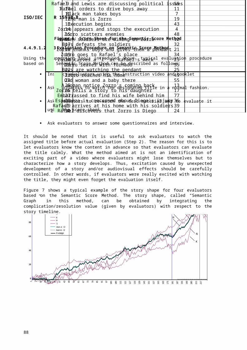
ISO/IEC PDTR 15938-8
<Title xml:lang="es">Telediario (segunda edición)</Title>
<Title xml:lang="en" type="popular">Afternoon news</Title>
<Title xml:lang="es" type="popular">Noticias de la tarde</Title>
<Abstract><FreeTextAnnotation>
The trial about the kidnapping of Segundo Marey started this morning. Short interview with Segundo Marey after the end of the first session.
</FreeTextAnnotation><StructuredAnnotation>
<Who><Name>Segundo Marey</Name>
</Who></StructuredAnnotation>
</Abstract><Creator>
<Role href="urn:mpeg:mpeg7:cs:RoleCS:2001:ANCHOR"><Name xml:lang="en">Anchorman</Name>
</Role><Agent xsi:type="PersonType">
<Name><GivenName>Ana</GivenName><FamilyName>Blanco</FamilyName>
</Name></Agent>
</Creator><CreationCoordinates>
<Location><Name xml:lang="es">Piruli</Name><Region>es</Region><AdministrativeUnit>Madrid</AdministrativeUnit>
</Location><Date>
<TimePoint>1998-10-03T14:13+01:00</TimePoint></Date>
</CreationCoordinates><CreationTool>
<Tool><Name>Video Camera</Name>
</Tool><Setting name="zoom" value="1.5"/><Setting name="aperture" value="35"/>
</CreationTool></Creation><Classification>
<Form href="urn:mpeg:mpeg7:cs:FormatCS:2001:1.1"><Name xml:lang="en">Bulletin</Name>
</Form><Genre href="urn:mpeg:mpeg7:cs:ContentCS:2001:1.3.1">
<Name xml:lang="en">Daily news</Name></Genre><Purpose href="urn:mpeg:mpeg7:cs:IntentionCS:2001:2.1">
<Name xml:lang="en">Pure information</Name></Purpose><Language type="original">es</Language><Release date="1998-06-16T21:30+01:00">
<Region>es</Region>
90

ISO/IEC PDTR 15938-8
</Release><ParentalGuidance>
<ParentalRating
href="urn:mpeg:mpeg7:cs:MPAAParentalRatingCS:2001:G"/><Region>es</Region>
</ParentalGuidance><MediaReview>
<Rating><RatingValue>10</RatingValue><RatingScheme best="10" worst="1"
style="higherBetter"><Name>Overall</Name>
</RatingScheme></Rating>
</MediaReview><MediaReview>
<FreeTextReview xml:lang="en">Interesting News today.
</FreeTextReview><FreeTextReview xml:lang="es">Interesantes noticias
hoy.</FreeTextReview><ReviewReference>
<DisseminationFormat
href="urn:mpeg:mpeg7:cs:DisseminationFormatCS:2001:4"><Name xml:lang="en">Internet</Name>
</DisseminationFormat><MediaLocator>
<MediaUri>http://tvmagazine.com</MediaUri></MediaLocator>
</ReviewReference></MediaReview>
</Classification><RelatedMaterial>
<DisseminationFormat
href="urn:mpeg:mpeg7:cs:DisseminationFormatCS:2001:4"/><MaterialType>
<Name xml:lang="en">Broadcaster Web Page</Name></MaterialType><MediaLocator>
<MediaUri>http://www.rtve.es</MediaUri></MediaLocator>
</RelatedMaterial></CreationInformation>
</Video></MultimediaContent>
</Description></Mpeg7>
4.6.2.5.2 Additional language description examples
In the following example, the original spoken audio of the multimedia content is in English; however, the content includes dubbed audio tracks in French and Spanish.
<CreationInformation><!-- more elements here -->
91

ISO/IEC PDTR 15938-8
<Classification><Language type="original">en</Language><Language type="dubbed">es</Language><Language type="dubbed">fr</Language>
</Classification></CreationInformation>
The following example is a description of a program broadcasted by a French TV station. The interview was originally done in Spanish and dubbed to English for a program produced and broadcasted in England. After dubbing, the Spanish can still be heard in the background. The interview was bought by the French TV station, which added subtitles in French for its broadcast.
<CreationInformation><!-- more elements here -->
<Classification><Language type="dubbed">en</Language><Language type="background">es</Language><CaptionLangauge closed="false">fr</CaptionLanguage>
</Classification></CreationInformation>
92
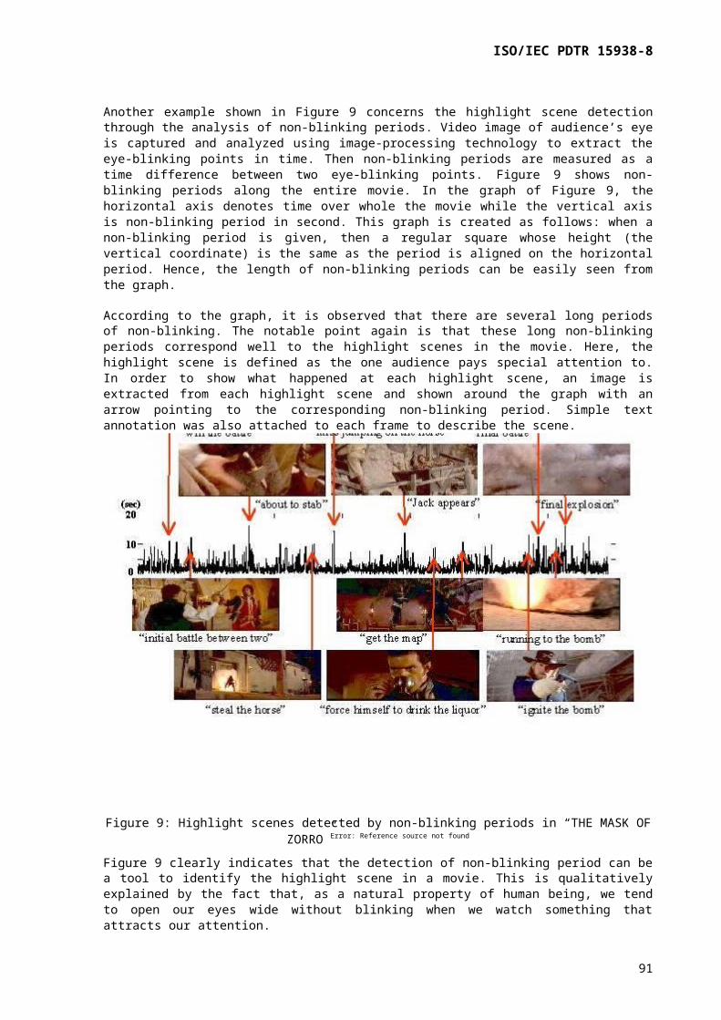
ISO/IEC PDTR 15938-8
4.7 Usage description tools
4.7.1 Introduction
This clause specifies tools describing information about the usage of the multimedia content. The following tools are specified in this clause:
Table 9: Overview of Usage Information Tools.Tool Functionality
Usage Tools These tools describe the information about the usage of the multimedia content. The UsageInformation DS include a Rights D, zero or one FinancialResults D, and several Availability DSs and associated UsageRecord DSs.
The Rights D contains references to rights holders in order to obtain rights information. The FinancialResults D contains the description of costs and incomes generated by the multimedia content. The Availability DS describes the details about the availability of the multimedia content for usage. The UsageRecord DS describes the details pertaining to the usage of the multimedia content.
It is important to note that the UsageInformation DS description will incorporated new descriptions each time the multimedia content is used (e.g, UsageRecord DS, Income in FinancialResults D), or when there are new ways to access to the multimedia content (Availability DS).
4.7.2 Usage information tools
4.7.2.1 UsageInformation DS
Information on extraction and use is not provided.
4.7.2.2 Rights datatype
Information on extraction and use is not provided.
4.7.2.3 Financial datatype
Information on extraction and use is not provided.
4.7.2.4 Availability DS
Information on extraction and use is not provided.
4.7.2.5 UsageRecord DS
Information on extraction and use is not provided.
4.7.2.6 Usage information examples
<Mpeg7><Description xsi:type="ContentEntityType">
<MultimediaContent xsi:type="VideoType">
93

ISO/IEC PDTR 15938-8
<Video><UsageInformation id="news1_usage">
<Rights><RightsID organization="TVE" type="TVECopyRightsID">
tve:19980618:td2</RightsID>
</Rights><FinancialResults>
<AccountItem currency="EUR" value="423.46"><CostType>
<Name>Total for production</Name></CostType>
</AccountItem><AccountItem currency="EUR" value="200">
<CostType><Name>Broadcast</Name>
</CostType></AccountItem><AccountItem currency="EUR" value="600">
<IncomeType><Name>Advertisment</Name>
</IncomeType></AccountItem>
</FinancialResults><Availability id="live_news1">
<InstanceRef idref="onlinemp7cs17news1"/><Dissemination>
<Format
href="urn:mpeg:mpeg7:cs:DisseminationFormatCS:2001:4"><Name xml:lang="en">Internet</Name>
</Format><Location>
<Region>es</Region></Location>
</Dissemination><Financial>
<AccountItem currency="EUR" value="1"><CostType>
<Name>Pay-per-view price</Name></CostType>
</AccountItem></Financial><AvailabilityPeriod type="payPerUse">
<TimePoint>1998-06-16T21:00+01:00</TimePoint><Duration>PT30M</Duration>
</AvailabilityPeriod></Availability><Availability id="repeated_news1">
<InstanceRef href="http://www.rtve.es/19980616/td2.mpeg"/>
<Dissemination><Format
href="urn:mpeg:mpeg7:cs:DisseminationFormatCS:2001:1"><Name>Terrestrial</Name>
</Format><Disseminator>
<Role href="urn:mpeg:mpeg7:cs:RoleCS:2001:PUBLISHER"/>
<Agent xsi:type="OrganizationType">
94
ISO/IEC PDTR 15938-8
<Name>Discovery Channel</Name></Agent>
</Disseminator><Location>
<Region>es</Region></Location>
</Dissemination> <AvailabilityPeriod type="repeat">
<TimePoint>1998-06-16T21:30+01:00</TimePoint></AvailabilityPeriod>
</Availability><UsageRecord>
<AvailabilityRef idref="live_news1"/><Audience>245747</Audience><Financial>
<AccountItem currency="EUR" value="1"><EffectiveDate>1998-06-16</EffectiveDate><IncomeType>
<Name>Income for pay-per-view live access</Name>
</IncomeType></AccountItem>
</Financial></UsageRecord>
</UsageInformation></Video>
</MultimediaContent></Description>
</Mpeg7>
95

ISO/IEC PDTR 15938-8
4.8 Structure description tools
4.8.1 Introduction
This clause specifies tools for describing the structure of multimedia content. These tools describe the following:
Images and spatial regions of images and video frames;
Video, temporal segments, and spatio-temporal segments of video;
Audio and temporal segments of audio;
Audio-visual content and spatio-temporal segments of AV content;
Multimedia content and segments of multimedia content;
Visual text in images or video;
Video mosaics;
Edited video and segments of edited video;
4.8.1.1 Structure description example
Figure 12 shows an example of the use of the structure description tools for describing a video. In this example, the video is described using the VideoSegment DS (top). The temporal decomposition of the video into two video segments is described using the VideoSegmentTemporalDecomposition DS. The specific attributes of the different video segments are described using the segment attribute description tools. The following tools are used to describe the attributes of the whole video (top): CreationInformation DS, MediaInformation DS, UsageInformation DS, and Semantic DS. The following tools are used to describe the attributes of the video segment on the left: TextAnnotation datatype, MediaTime datatype, MotionActivity D, and other visual Ds. The following tools are used to describe the video segment on the right: TextAnnotation datatype, SpatioTemporalMask D, and other visual Ds.
96

ISO/IEC PDTR 15938-8
Figure 12: Illustration of the description of a video segment using tools for describing the structure of multimedia content.
4.8.2 Base segment description tools
4.8.2.1 Segment DS
Information on extraction and use is not provided.
4.8.2.2 Base segment decomposition tools
Information on extraction and use is not provided.
4.8.3 Segment attribute description tools
4.8.3.1.1 Mask D
Information on extraction and use is not provided.
4.8.3.1.2 SpatialMask D
4.8.3.1.2.1 SpatialMask D examples
The following example illustrates the use of the SpatialMask D for describing the spatial mask that consists of three spatially connected sub-regions. Each sub-region is described using a polygon that denotes its boundary.
<SpatialMask>
97

ISO/IEC PDTR 15938-8
<SubRegion><Polygon>
<Coords mpeg7:dim="2 5"> 5 25 10 20 15 15 10 10 5 15 </Coords></Polygon>
</SubRegion><SubRegion>
<Polygon><Coords mpeg7:dim="2 6"> 7 24 15 24 20 27 18 25 15 22 7 22
</Coords></Polygon>
</SubRegion><SubRegion>
<Polygon><Coords mpeg7:dim="2 4"> 7 30 15 30 15 25 7 25</Coords>
</Polygon></SubRegion>
</SpatialMask>
4.8.3.1.3 TemporalMask D
4.8.3.1.3.1 TemporalMask D examples
The following example illustrates the use of the TemporalMask D for describing the temporal mask that consists of two temporally connected sub-intervals. Each sub-interval is described using a media time description (time point and duration) that denotes its boundaries in time.
<TemporalMask><SubInterval>
<MediaTimePoint>T00:00:00</MediaTimePoint><MediaDuration>PT6M</MediaDuration>
</SubInterval><SubInterval>
<MediaTimePoint>T00:07:00</MediaTimePoint><MediaDuration>PT3M</MediaDuration>
</SubInterval></TemporalMask>
4.8.3.1.4 SpatioTemporalMask D
4.8.3.1.4.1 SpatioTemporalMask D examples
The following example illustrates the use of the SpatioTemporalMask D for describing a spatio-temporal mask comprised of two spatio-temporal sub-regions. Each sub-region is described by trajectories of the representative points of a reference region using a spatio-temporal locator description.
<SpatioTemporalMask><SubRegion>
<FigureTrajectory type="rectangle"><MediaTime>
<MediaTimePoint>T00:00:15</MediaTimePoint><MediaDuration>PT1M15S</MediaDuration>
</MediaTime><Vertex><!-- more elements here --></Vertex><Vertex><!-- more elements here --></Vertex><Vertex><!-- more elements here --></Vertex><!-- more elements here -->
98

ISO/IEC PDTR 15938-8
</FigureTrajectory></SubRegion><SubRegion>
<FigureTrajectory type="ellipse"><MediaTime>
<MediaTimePoint>T00:14:00</MediaTimePoint><MediaDuration>PT1M7S</MediaDuration>
</MediaTime><Vertex><!-- more elements here --></Vertex><Vertex><!-- more elements here --></Vertex><Vertex><!-- more elements here --></Vertex><!-- more elements here -->
</FigureTrajectory></SubRegion>
</SpatioTemporalMask>
4.8.3.1.5 MediaSpaceMask D
4.8.3.1.5.1 MediaSpaceMask D examples
The following example illustrates the use of the MediaSpaceMask D for describing a media space mask consisting of two sub-intervals from the media stream shown in Figure 13.
<MediaSpaceMask><SubInterval offset="105" length="34"/><SubInterval offset="167" length="50"/>
</MediaSpaceMask>
Figure 13: Example of a media space mask.
4.8.3.1.6 SceneGraphMask D
4.8.3.1.6.1 SceneGraphMask D examples
The following example illustrates the use of the SceneGraphMask D for describing a scene graph mask comprised of two sub-graphs (#1 and #21) from the scene graph shown in Figure 14.
<SceneGraphMask><SubGraphNum>1</SubGraphNum><SubGraphNum>21</SubGraphNum>
</SceneGraphMask>
99

ISO/IEC PDTR 15938-8
Figure 14: Example of a scene graph mask.
4.8.3.1.7 OrderedGroupDataSetMask D
4.8.3.1.7.1 OrderedGroupDataSetMask D example
The following example illustrates the use of the OrderedGroupDataSetMask D for describing an ordered group data set mask consisting of two sub-intervals as shown in Figure 15. This example organizes ink content by grouping ink strokes into ordered group data sets. Each ordered group data set consists of ink strokes to form the component layer, and each stroke consists of ink data points to form the unit layer.
<OrderedGroupDataSetMask><SubInterval setRef="http://www…/demo.stk#1" startComponent="0"
startUnit="0"endComponent="0" endUnit="U"/>
<SubInterval setRef="http://www…/demo.stk#Set_N" startComponent="1" startUnit="0"
endComponent="1" endUnit="V"/></OrderedGroupDataSetMask>
Figure 15: Example of an ordered group mask.
4.8.3.2 MatchingHint D
4.8.3.2.1 MatchingHint D examples
The following example illustrates the use of the MatchingHint D for describing relative importance values to the several instances of visual description tools in a StillRegion DS description.
100

ISO/IEC PDTR 15938-8
<StillRegion id="IMG0001"><MatchingHint reliability="0.900000">
<Hint value="0.455" xpath="../../../ColorStructure"/><Hint value="0.265" xpath="../../../DominantColor"/><Hint value="0.280" xpath="../../../HomogeneousTexture"/>
</MatchingHint>
<VisualDescriptor xsi:type="DominantColorType"><!-- more elements here -->
</VisualDescriptor><VisualDescriptor xsi:type="ColorStructureType">
<!-- more elements here --></VisualDescriptor><VisualDescriptor xsi:type="HomegeneousTextureType">
<!-- more elements here --></VisualDescriptor><!-- more elements here -->
</StillRegion>
MatchingHint D descriptions can be generated and updated continuously by user’s feedback. The reliability of the importance values may vary depending on how the values have been updated. For example, matching hint values learned from a large number of feedback sessions from reliable experts will have higher reliability.
4.8.3.2.2 MatchingHint D extraction
There is no limitation in the extraction methods for the MatchingHint D. But the automatic extraction method by relevance feedback can work well on extracting the values of the DS. Relevance feedback is a feedback from a user regarding what is relevant and/or irrelevant results from a given retrieval output. In this subclause, the automatic extraction method for MatchingHints is described.
The MatchingHints can be automatically extracted using the learning algorithm based on the clustering information where similar data are grouped together. This clustering information can be given by a service provider or can be built-up by user’s relevance feedback. By using the extracted MatchingHints, the retrieval system can retrieve similar data even which is not used in the MatchignHint training. The descriptor that classifies the data in the same cluster better has the higher hint value and the descriptor which misclassifies the data in different clusters into the same cluster has the lower hint value. The hint value can be learned continuously if there are more feedbacks. To prevent wrong learning from the wrong feedback, the reliability factor describing how reliable the hint values are is used. In other words, the reliability describes how stable the current hint values are. The reliability becomes high when there are frequent feedbacks from the known experts. The higher the reliability is, the less a feedback affects the current hint value.
The equation of the learning MatchingHint D value follows as:
101

ISO/IEC PDTR 15938-8
The system calculates matching hints with the feedback, and updates and stores matching hints of an image (or a part of a video). Updating matching hints (Wnew) are based on the matching hints (Wt) currently stored in the image (or the part of a video) and the matching hints (Wc) derived from feedback, as shown in the above equation. In the equation, updated matching hint (Wnew) is affected by Wt and Wc in proportion to the current reliability and the effect value. In other words, the updated matching hint (Wnew) is more affected by Wt when the reliability is higher, and more affected by Wc
when the effect value is higher. The effect value, ec is high when the user giving feedback is the expert authorized, but generally, it is fixed as a constant.
The matching hints Wc can be calculated by the following equation from the feedback. If feedback is a relevant image, then a matching hint of a descriptor becomes higher when the similarity calculated using this descriptor is high. On the contrary, in the case of an irrelevant image, a matching hint of a descriptor becomes higher when the distance calculated using this descriptor is high.
Reliability is updated by the following equation. The reliability becomes high when there is frequent feedback and continuous increase of performance by learning
Rnew=f(Rold+e(IncreaseTerm+a))
IncreaseTerm=(Precision(t)-Precision(t-1))
Rnew : new updated reliability
Rold : current reliability
e :effect coefficient
a : constant value
Precision(t) : the precision calculated from feedback at the time t
Precision(t-1) : the precision calculated from feedback at the time t-1
f(): normalizing function
4.8.3.3 PointOfView D
4.8.3.3.1 PointOfView D examples
The following examples illustrate the use of the PointOfView D for describing the relative importance of AV segments given a specific viewpoint. In these examples, the AV segments belong to the video of a football game between Team A and Team B. The PointOfView D describes the viewpoints of "Team A" and "Team B". In this example, it is assumed that the content creator assigned the relative importance values to the AV segments manually using an authoring tool. The
102
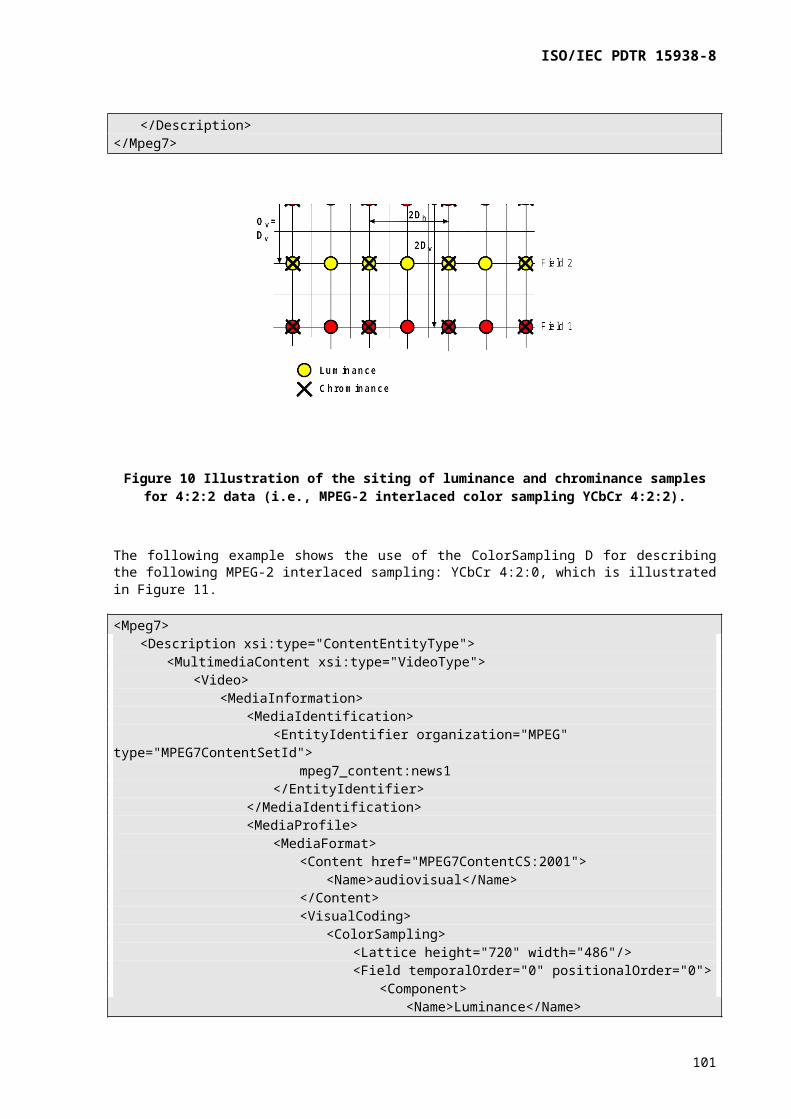
ISO/IEC PDTR 15938-8
examples show the description of the PointOfView D in the nested form and in the separated form, respectively.
In the first example, the description contains several PointOfView D descriptions with the same viewpoint "Team A". The importance values of the PointOfView D descriptions with viewpoint "Team A" included within the AudioVisualSegment DS descriptions with ids "seg1", "seg2", ..., "seg20", ... can be compared; the same is true within the AudioVisualSegment DS descriptions with ids of "seg1_2", "seg2_2", ..., "seg20_2", .... However, the importance values of PointOfView D descriptions across the two sets of AudioVisualSegment DS descriptions cannot be compared because they are of different scope.
<!-- Description of PointOfView D: nested form --><Mpeg7>
<Description xsi:type="ContentEntityType"><MultimediaContent xsi:type="AudioVisualType">
<AudioVisual><TemporalDecomposition>
<AudioVisualSegment id="FootBallGame"><TemporalDecomposition>
<AudioVisualSegment id="seg1"><PointOfView viewpoint="Team A">
<Importance><Value>0.3</Value>
</Importance></PointOfView><PointOfView viewpoint="Team B">
<Importance><Value>0.7</Value>
</Importance></PointOfView>
</AudioVisualSegment><AudioVisualSegment id="seg2">
<PointOfView viewpoint="Team A"><Importance>
<Value>0.5</Value></Importance>
</PointOfView></AudioVisualSegment><!-- more elements here --><AudioVisualSegment id="seg20">
<PointOfView viewpoint="Team A"><Importance>
<Value>0.8</Value></Importance>
</PointOfView><PointOfView viewpoint="Team B">
<Importance><Value>0.2</Value>
</Importance></PointOfView>
</AudioVisualSegment><!-- more elements here -->
</TemporalDecomposition><TemporalDecomposition>
<AudioVisualSegment id="seg1_2"><PointOfView viewpoint="Team A">
<Importance><Value>0.3</Value>
</Importance></PointOfView>
</AudioVisualSegment>
103

ISO/IEC PDTR 15938-8
<AudioVisualSegment id="seg2_2"><PointOfView viewpoint="Team A">
<Importance><Value>0.5</Value>
</Importance></PointOfView>
</AudioVisualSegment><!-- more elements here --><AudioVisualSegment id="seg20_2">
<PointOfView viewpoint="Team A"><Importance>
<Value>0.8</Value></Importance>
</PointOfView></AudioVisualSegment><!-- more elements here -->
</TemporalDecomposition></AudioVisualSegment>
</TemporalDecomposition></AudioVisual>
</MultimediaContent></Description>
</Mpeg7>
In the second example, the scope of each PointOfView D description is each description itself.
<Mpeg7><Description xsi:type="ContentEntityType">
<MultimediaContent xsi:type="AudioVisualType"><AudioVisual>
<TemporalDecomposition><AudioVisualSegment id="FootBallGame">
<!-- Description of PointOfView D: separated form --><PointOfView viewpoint="Team A">
<Importance><Value>0.3</Value><SegmentRef href="#seg1"/>
</Importance><Importance>
<Value>0.5</Value><SegmentRef href="#seg2"/>
</Importance><!-- more elements here --><Importance>
<Value>0.8</Value><SegmentRef href="#seg20"/>
</Importance><!-- more elements here -->
</PointOfView><PointOfView viewpoint="Team B">
<Importance><Value>0.7</Value><SegmentRef href="#seg1"/>
</Importance><!-- more elements here --><Importance>
<Value>0.2</Value><SegmentRef href="#seg20"/>
</Importance><!-- more elements here -->
104

ISO/IEC PDTR 15938-8
</PointOfView><!-- Description of AV segment tree --><TemporalDecomposition>
<AudioVisualSegment id="seg1"><!-- more elements here -->
</AudioVisualSegment><AudioVisualSegment id="seg2">
<!-- more elements here --></AudioVisualSegment><!-- more elements here --><AudioVisualSegment id="seg20">
<!-- more elements here --></AudioVisualSegment><!-- more elements here -->
</TemporalDecomposition></AudioVisualSegment>
</TemporalDecomposition></AudioVisual>
</MultimediaContent></Description>
</Mpeg7>
4.8.3.3.2 PointOfView D use
The PointOfView D is a tool that allows generating a scalable summary dynamically. A scalable summary consists of the segments that have user’s preferred viewpoints. To achieve scalability of summary, the relative importance value and corresponding viewpoint is attached to each segment, and the segment filtering engine of the PointOfView D descriptions selects segments in order of high importance value for each viewpoint until the total time of summary becomes user’s demanding time period. The PointOfView D consists of the relative importance of segments and a specific viewpoint that is the axis of the relative importance.
The PointOfView D can be used to summarize multimedia content dynamically from the combination of the viewpoint(s) and the duration which user or agent or system required. The functionality of segment filtering, which can be enabled by PointOfView D, can be used as a preprocessor for the Summarization DS to make summary descriptions. The PointOfView D can also be used for scalable multimedia distribution by generating different multimedia presentations that consist of the filtered (preferred) segments, which can be adapted to the different capabilities of the client terminals, network conditions or user preferences, and so on.
A generic usage model is depicted in Figure 16 below, where a segment filter takes media description including PointOfView descriptions embedded in (or associated with) Segments as input and user preferences and generates a filtered output containing media or summary description that consists of preferred segments that fit personal preference.
105

ISO/IEC PDTR 15938-8
Figure 16: A generic usage model for PointOfView D descriptions.
4.8.4 Visual segment description tools
4.8.4.1 StillRegion DS
4.8.4.1.1 StillRegion DS examples
The following example illustrates the use of the StillRegion DS for describing the image shown in Figure 17. Various attributes of the image such as the location, annotation, and color are described using the following tools, respectively: MediaLocator datatype, the TextAnnotation datatype, and the ScalableColor D (defined in ISO/IEC 15938-3).
Figure 17: Example of an image showing two people shaking hands. The image is described using the StillRegion DS.
<StillRegion><MediaLocator>
<MediaUri>image.jpg</MediaUri></MediaLocator><TextAnnotation>
<FreeTextAnnotation> Alex shakes hands with Ana </FreeTextAnnotation>
</TextAnnotation><VisualDescriptor xsi:type="ScalableColorType" numOfCoeff="16"
numOfBitplanesDiscarded="0"><Coeff> 1 2 3 4 5 6 7 8 9 0 1 2 3 4 5 6 </Coeff>
</VisualDescriptor></StillRegion>
4.8.4.1.2 StillRegion DS extraction
Still regions cab be the result of a spatial segmentation or a spatial decomposition methods. This may be done automatically or by hand, based on semantics criteria or not. Several techniques are reported in , . Note that this kind of analysis tools have been extensively studied in the framework of the MPEG-4 standard. Some examples are described in , , . This subclause describes one example proposed in .
The extraction of individual spatial or temporal regions and their organization within a tree structure can be viewed as a hierarchical segmentation problem also known as a partition tree creation. The strategy presented here involves three steps illustrated in Figure 18: the first step is a conventional segmentation. Its goal is to produce an initial partition with a rather high level of details. Depending on the nature of the segment tree, this initial segmentation can be a shot detection algorithm (for VideoSegment DS) or a spatial segmentation following a color homogeneity criterion (for StillRegion DS). The second step is the creation of a Binary Partition Tree. Combining the segments (VideoSegment or StillRegion DSs) created in the first step, the Binary Partition Tree defines the set of segments to be indexed and encodes their similarity with the help of a binary tree. Finally, the third
106

ISO/IEC PDTR 15938-8
step restructures the binary tree into an arbitrary tree. Although the approach can be used for many types of segments, the following description assumes still regions.
Figure 18: Outline of segment tree creation.The first step is rather classical (see and the reference herein for example). The second step of the Segment tree creation is the computation of a Binary Partition Tree. Each node of the tree represents connected components in space (regions). The leaves of the tree represent the regions defined by the initial segmentation step. The remaining nodes represent segments that are obtained by merging segments represented by the children. This representation should be considered as a compromise between representation accuracy and processing efficiency. Indeed, all possible merging of initial segments are not represented in the tree. Only the most "useful'' merging steps are represented. However, the main advantage of the binary tree representation is that efficient techniques are available for its creation and it conveys enough information about segment similarity to construct the final tree. The Binary Partition Tree should be created in such a way that the most "useful'' segments are represented. This issue can be application dependent. However, a possible solution, suitable for a large number of cases, is to create the tree by keeping track of the merging steps performed by a segmentation algorithm based on merging. This information is called the merging sequence. The process is illustrated in Figure 19. The original partition involves four regions. The regions are indicated by a letter and the number indicates the mean gray level value. The algorithm merges the four regions in three steps.
Figure 19: Example of Binary Partition Tree creation with a region merging algorithm.To create the Binary Partition Tree, the merging algorithm may use several homogeneity criteria based on low-level features. For example, if the image belongs to a sequence of images, motion information can be used to generate the tree: in a first stage, regions are merged using a color homogeneity criterion, whereas a motion homogeneity criterion is used in the second stage. Figure 20 presents an example of a Binary Partition Tree created with color and motion criteria for the Foreman sequence. The nodes appearing in the lower part of the tree as white circles correspond to the color criterion, whereas the dark squares correspond to the motion criterion. As can be seen, the process starts with a color criterion and then, when a given Peak Signal to Noise Ratio (PSNR) is reached, it changes to the motion criterion. Regions that are homogeneous in motion as the face and helmet are represented by a single node (B) in the tree.
107

ISO/IEC PDTR 15938-8
Figure 20: Examples of creation of the Binary Partition Tree with color and motion homogeneity criteria.
Furthermore, additional information about previous processing or detection algorithms can also be used to generate the tree in a more robust way. For instance, an object mask can be used to impose constraints on the merging algorithm in such a way that the object itself is represented as a single node in the tree. Typical examples of such algorithms are face, skin, character or foreground object detection. An example is illustrated in Figure 21. Assume for example that the original Children sequence has been analyzed so that masks of the two foreground objects are available. If the merging algorithm is constrained to merge regions within each mask before dealing with remaining regions, the region of support of each mask will be represented as a single node in the resulting tree. In Figure 21 the nodes corresponding to the background and the two foreground objects are represented by squares. The three sub-trees further decompose each object into elementary regions.
Figure 21: Example of partition tree creation with restriction imposed with object masks.The purpose of the third and last step of the algorithm is to restructure the Binary Partition Tree into an arbitrary tree that shall reflect more clearly the image structure. To this end, nodes that have been created by the binary merging process but do not convey any relevant information should be removed. The criterion used to decide if a node must appear in the final tree can be based on the variation of segments homogeneity. A segment is kept in the final tree if the homogeneity variation between itself and its parent is low. Furthermore, techniques pruning the tree can be used since not all regions may have to be described. Finally, a specific GUI can also be designed to manually modify the tree to keep the useful sets of segments. An example of simplified and restructured tree is shown in Figure 22.
Figure 22: Example of restructured tree.
108

ISO/IEC PDTR 15938-8
4.8.4.2 Still region decomposition tools
4.8.4.2.1 Still region decomposition tools examples
The following example illustrates the use of the StillRegionSpatialDecomposition DS in the StillRegion DS for describing the spatial decomposition of the image in Figure 17 into two still regions shown in Figure 23. In this example, the still region with id = "AlexAnaSR" corresponds to the full image from which two still regions, id = "AlexSR" and id = "AnaSR" are generated by spatial segmentation. In this example, each still region segment, id = "AlexSR", and id = "AnaSR", correspond to a person in the image. In this example, the segment decomposition has gaps (gaps = true) but no overlaps (overlap = false). The two still regions are spatially connected. The TextAnnnotation describes an annotation of each still region. The ScalableColor D (defined in ISO/IEC 15938-3) describes the contour shape of each still region.
Figure 23: Example of the spatial decomposition of an image into two still regions.
<Mpeg7><Description xsi:type="ContentEntityType">
<MultimediaContent xsi:type="ImageType"><Image>
<SpatialDecomposition gap="true" overlap="false"><StillRegion id="AlexSR">
<TextAnnotation><FreeTextAnnotation> Alex </FreeTextAnnotation>
</TextAnnotation><VisualDescriptor xsi:type="ScalableColorType"
numOfCoeff="16" numOfBitplanesDiscarded="0"><Coeff> 1 2 3 4 5 6 7 8 9 0 1 2 3 4 5 6 </Coeff>
</VisualDescriptor></StillRegion><StillRegion id="AnaSR">
<TextAnnotation><FreeTextAnnotation> Ana </FreeTextAnnotation>
</TextAnnotation><VisualDescriptor xsi:type="ScalableColorType"
numOfCoeff="16" numOfBitplanesDiscarded="0"><Coeff> 1 2 3 4 5 6 7 8 9 0 1 2 3 4 5 6 </Coeff>
</VisualDescriptor></StillRegion>
</SpatialDecomposition>
Sti llR egi on
S ti llR egi onS t ill Reg ion
S t ill Reg ionSpat ia lDe com po sit ion
109

ISO/IEC PDTR 15938-8
</Image></MultimediaContent>
</Description></Mpeg7>
4.8.4.3 ImageText DS
4.8.4.3.1 ImageText DS examples
The following example illustrates the use of the ImageText DS for describing the image text of the image shown in Figure 24. The image contains one instance of scene image text ("Cherie, je suis la") and two instances of superimposed image text ("En direct du stade DE-KUIP Rotterdam Jean-Francois DEVELEY" and "Nous allons assister a un match fantastique").
Figure 24: Example of an image that contains image text.
<Mpeg7><Description xsi:type="ContentEntityType">
<MultimediaContent xsi:type="ImageType"><Image>
<SpatialDecomposition gap="true" overlap="false"><StillRegion xsi:type="ImageTextType" textType="scene">
<SpatialLocator><!-- more elements here -->
</SpatialLocator><Text xml:lang="fr"> Cherie, je suis la </Text>
</StillRegion><StillRegion xsi:type="ImageTextType"
textType="superimposed" fontSize="40" fontType="Arial"><SpatialLocator>
<!-- more elements here --></SpatialLocator><Text xml:lang="fr">
En direct du state DE-KUIP Rotterdam Jean-Francois DEVELEY </Text>
</StillRegion><StillRegion xsi:type="ImageTextType"
textType="superimposed" fontSize="30" fontType="Times New Roman"><SpatialLocator>
<!-- more elements here -->
CH E RIEJE S U IS L A
Nous al lons assister a un match fan tastique
En direct dustade DE -KUIPRo tter dam J ean -Francois DEVELEY
sce ne text
supe rim po sed text
supe rim po sed text
(cap ti ons)
110

ISO/IEC PDTR 15938-8
</SpatialLocator><Text xml:lang="fr">
Nous allons assister a un match fantastique </Text></StillRegion>
</SpatialDecomposition></Image>
</MultimediaContent></Description>
</Mpeg7>
4.8.4.4 Mosaic DS
4.8.4.4.1 Mosaic DS examples
The following example illustrates the use of the Mosaic DS for describing the mosaic of a video segment.
<Mosaic><!-- Affine model, Center of Source --><WarpingParam modelType="6"
sourceSequenceWidth="352"sourceSequenceHeight="288"xOffset="2" yOffset="7"xOrigin="176" yOrigin="144">
<MediaTimePoint> <!-- more elements here --> </MediaTimePoint><MotionParam> 0.0 0.0 0.0 0.0 0.0 0.0 </MotionParam><MediaTimePoint> <!-- more elements here --> </MediaTimePoint><MotionParam> -3.60 0.73 0.03 0.01 0.01 0.51 </MotionParam><!—- more elements here -->
</WarpingParam></Mosaic>
A mosaic allows the representation and visualization of a video segment using a single image. This functionality can also be provided by key frames. However, a mosaic contains more visual information than a key frame (e.g., motion warping parameters), but is not suitable for all kinds of shots (e.g., shots with rapidly changing background). Thus, mosaics and key frames serve complementary functions. Mosaics can also be useful for performing searching of video segments. Image features can be extracted from the mosaic image to describe the features of the video segment. Moreover, since the Mosaic DS extends the StillRegion DS, the StillRegionSpatialDecomposition DS can be used to describe the decomposition of a mosaic into still regions, each of which can be described individually. The warping information an also be used for summarizing the video segment since it describes the global motion in the segment. The mosaics may also be useful for video editing since the mosaics can be easily manipulated, using common image processing tools, and then resconstructing the video segment from the manipulated mosaic image.
4.8.4.4.2 Mosaic DS extraction
It is very important to be able to construct good mosaics even from video shots that are not pre-segmented, videos with lots of free moving objects and videos where motion is large and subsequent frames therefore are largely disaligned. Thus a very stable and robust algorithm is important for handling these situations. The algorithm described below is described in detail in . Below a brief description is given.
As input to a mosaic algorithm is a set of video frames and as the final output there is the resulting mosaic image of these frames. Generally, the mosaicing procedure can be divided into two main parts. First the set of frames have to be aligned with each other, and then follows the construction of the mosaic where the data is merged into one single image.
111

ISO/IEC PDTR 15938-8
The merging can be done with several criteria, for instance averaging of the frame data or pasting with the latest frame. But before the merging can be done, alignment of the frames has to be performed, and the method of alignment is critical for the quality and robustness of the algorithm.
The aim when developing a mosaic construction method has been to make an algorithm that is robust and reliable, well prepared to deal with unsegmented video containing free-moving objects and large frame disalignment. In order to achieve this, the algorithm is based on minimization of an error measure for the alignment of the frames.
This alignment process between frames is described in detail in the Visual XM in the context of the Parametric Motion Descriptor. When all frames have been aligned, the mosaic can be constructed by merging the data from all frames into the same reference system. Generally in the entire algorithm, if masks are present, only data that are not masked out is used in the calculations.
4.8.4.5 StillRegion3D DS
Information on extraction and use is not provided.
4.8.4.6 3D still region decomposition tools
Information on extraction and use is not provided.
4.8.4.7 VideoSegment DS
4.8.4.7.1 VideoSegment DS examples
The following examples illustrate the use of the VideoSegment DS for describing the video shown in Figure 12. In this example, the video segment id ="RootVS" represents the full video. The MediaTime describes the time information for the segment. The GoFGoPColor D (defined in ISO/IEC 15938-3) describes the color information of the video segment.
<VideoSegment id="RootVS"><MediaTime>
<MediaTimePoint>T00:00:00</MediaTimePoint><MediaDuration>PT1M30S</MediaDuration>
</MediaTime><VisualDescriptor xsi:type="GoFGoPColorType" aggregation="Average">
<ScalableColor numOfCoeff="16" numOfBitplanesDiscarded="0"><Coeff> 1 2 3 4 5 6 7 8 9 0 1 2 3 4 5 6 </Coeff>
</ScalableColor></VisualDescriptor>
</VideoSegment>
4.8.4.7.2 VideoSegment DS extraction
Video segments can be the result of a temporal segmentation methods. This may be done automatically or by hand, based on semantics or other criteria. An overview of temporal segmentation can be found in , and . This subclause describes an automatic method for detecting scene changes in MPEG-2 streams, which results in the temporal segmentation of video sequences into scenes.
This scene change detection algorithm is formed based on the statistical characteristics of the DCT DC coefficient values and motion vectors in the MPEG-2 bitstream. First, the algorithm detects candidate scene change on I, P, and B-frames separately, and dissolved editing effects. Then, a final decision is made to select the true scene changes. The overall scene change detection algorithm has five stages: minimal decoding, parsing, statistical detection, and decision stages; these five stages are described below. Figure 25 shows the block diagram of each stage.
112

ISO/IEC PDTR 15938-8
Figure 25: The Block diagram of the scene change detection algorithm.
Minimal Decoding Stage: The MPEG bitstream is partially decoded to obtain motion vectors and the DCT DCs.
Parsing Stage: The motion vectors in B, and P frames are counted; the DCT DC coefficients in P frames are reconstructed.
Statistical Stage:
1. Compute R p, the ratio of intra coded blocks and forward motion vectors in P-frames.
2. Compute R b, the ratio of backward and forward motion vectors in B-frames.
3. Compute R f, the ratio of forward and backward motion vectors in B-frames.
4. Compute the variance of DCT DC coefficients of the luminance in I and P frames.
Detection Stage:
1. Detect R p peaks in P frames and mark them as candidate scene change frames.
2. Detect R b peaks in B frames and mark them as candidate scene change frames.
3. Detect R f peaks in B frames. Detect all |Ds2|, absolute value of the frame intensity variance difference, in I, P frames. Mark I-frames as candidate scene change frames if they have |Ds2| peaks and if the immediate B-frames have R f peaks.
4. Detect the parabolic variance curve for dissolve effects.
Decision Stage:
1. All candidate frames that fall in the dissolve region are unmarked.
2. Search through all marked frames from the lowest frame number
if (current marked frame number - last scene change number) > T rejection,
then current marked frame is a true scene change
else unmark current frame
(where T rejection is the rejection threshold, default one GOP.)
113

ISO/IEC PDTR 15938-8
The criterion in step 2 of the Decision Stage is used to eliminate situations when a scene change happens on a B frame, then the immediately subsequent P-frame and/or I-frame (of display order) will likely be marked as candidate scene change as well. But since they don’t satisfy the criterion of "the minimum distance between two scene changes has to be greater than T rejection", these candidate frames will be unmarked. Situations where multiple scene changes occur on one GOP are very rare.
For P frames, the marked frame decision can be obtained both from step 1 (R p peaks) and step 3 (|Ds2| peaks) in the Detection Stage. The outcome from step 1 is usually more reliable. The outcome from step 3 can be used as reference if they are conflicting with the outcome of step 1.
The following subclauses describe a technique for detecting the peak ratios R b , R p and R f, and a method to detect dissolves.
4.8.4.7.2.1Adaptive Local Window Threshold Setting Technique for Detecting Peak Ratios
Different scenes have very different motion vector ratios. But within the same scene, they tend to be similar. Setting several levels of global thresholds will not only complicate the process but will also cause false alarms and false dismissals. A local adaptive threshold technique is used to overcome this problem.
The peak ratios R b , R p and R f are detected separately. All ratios are first clipped to a constant upper limit, usually 10 to 20. Then ratio samples are segmented into time windows. Each window is 2 to 4 times the Group of Picture (GOP)’s size. For typical movie sequences, scene change distances are mostly greater than 24 frames, so a window size of 2 GOP is sufficient. If the GOP is 12 frames, and window size is 2 frames, there will be 6 ratio samples for P-frames and 12 samples for B-frame. These samples are enough to detect the peaks.
Within the window, a histogram of the samples with a bin size of 256 is calculated. If the peak-to-average ratio is greater than the threshold, Td , then the peak frame is declared as a candidate scene change. The peak values are not included in calculating the average. A typical Td value is 3 for R b , R p and R f . Figure 26b. shows the histogram of a local window corresponding to P-frames (from frames 24 to 47) in Figure 26a. where there is a peak at frame 29. For B-frames, if a scene change happens at a B-frame (frame 10, in Figure 26a.), then the ratio of the immediately subsequent B frame (frame 11) will be also high. Both of them will be considered as peaks and will not be considered into the average, only the first B-frame will be marked as a candidate scene change.
Figure 26: Motion Vector Ratio In B and P Frames.
4.8.4.7.2.2 Detection of Dissolves
Dissolve is the most frequently used editing effect to connect two scenes together. A dissolve zone is created by linearly mixing two scenes sequences: one gradually decreasing in intensity and another gradually increasing. Dissolves can be detected by taking the pixel domain intensity variance of each frame and then detecting a parabolic curve. Given an MPEG-2 bitstream, the variance of the DCT DC coefficients in I and P frames is calculated instead of the spatial domain variance. Experiments have shown that this approximation is accurate enough to detect dissolves.
114

ISO/IEC PDTR 15938-8
4.8.4.7.2.2.1 Calculation of DCT DC Coefficient Values
The I-frames in MPEG are all intra coded, so the DCT DC coefficient values can be obtained directly (without temporal prediction). The P-frames consist of backward motion compensated (MC) macroblocks and the intra coded macroblocks. An MC macroblock has a motion vector and a DCT coded MC prediction error. Each macroblock consists of 4 luminance blocks (8x8 pixels each) and some chrominance blocks (2, 6 or 8 depending on the chrominance subsampling format). To ensure maximum performance, only the DCT DC coefficients of the luminance macroblock are used for dissolve detection. The DCT DC coefficient values of B pictures could also be reconstructed applying the same technique.
To get the DCT DC coefficient values for a P frame, inverse motion compensation is applied on the luminance blocks and the DCT DC coefficient value of the prediction error is added to the DCT DC coefficient prediction. Assume that the variance within each block is small enough, then b, the DCT DC coefficient of a MC block in a P frame can be approximated by taking the area-weighted average of the four blocks in the previous frame pointed by the motion vector.
b = [b 0 *(8-x)*(8-y) + b 1 *x*(8-y) + b 2 *(8-x)*y + b 3 *x*y]/64 + b error_DCT_DC
where x, y are the horizontal and vertical motion vector modulo block size 8; b 0 , b 1 , b 2 and b 3 are the DCT DC coefficients of the four neighboring blocks pointed by the motion vector; b error_DCT_DC is the DCT DC coefficient of the motion compensation error of the block to be reconstructed (see Figure 27).
Figure 27: Inverse Motion Compensation of DCT DC coefficient.
4.8.4.7.2.2.2 Dissolve Detection
Two criteria are used for dissolved detection --first, the depth of the variance valley must be large enough and second, the MediaDuration of the candidate dissolve region must be long enough (otherwise it is more likely an abrupt scene change). A typical dissolve would last from 30 to 60 frames. The specific procedure is as following.
All the positive-peaks, p + are detected by using the local window method on Ds2, the frame variance difference; all the negative-peaks p - are found by detecting the minimum value between two positive-peaks; the peak-to-peak difference Dp = current peak - previous peak, is calculated and thresholded using the pro-posed local window method; finally potential matches with MediaDuration length (positive peak to current negative peak) long enough ( > T f frames, e.g. 1/3 of the minimum allowed dissolve MediaDuration) are declared as candidate dissolves.
The starting point of the candidate dissolve is the previous positive peak. If the next positive peak is at least T f frames from the current negative peak, then a dissolve is declared and the ending point is set to the next positive peak. Frames whose peak-to-peak distance meets the magnitude threshold, but fail to meet the MediaDuration threshold are usually the direct scene changes. Similarly, if the frame MediaDuration from the current negative peak to the next positive peak fails to meet T f , the candidate dissolve will be unmarked also.
115

ISO/IEC PDTR 15938-8
4.8.4.8 Video segment decomposition tools
4.8.4.8.1 Video segment decomposition tools examples
The following examples illustrate the use of the VideoSegmentTemporalDecomposition DS and VideoSegmentSpatioTemporalDecomposition DS for describing the temporal and spatio-temporal decomposition of a video segment.
The first example describes the segment decompositon shown in Figure 12. In this example, the video segment has two scenes, "Chase" and "Capture". The video segment id = "RootVS" is decomposed in two video segments, id = "ChaseVS" and id = "CaptureVS". The video segment id = "ChaseVS" corresponds to the scene "Chase", and video segment id = "CaptureVS" corresponds to the scene "Capture". The segment decomposition has neither gaps (gap = false) nor overlaps (overlap = false). The video segments are temporally connected. At the same time, the video segment "CaptureVS" is decomposed into two moving regions: id = "ManMR" and id = "WomanMR". The moving region id = "ManMR" corresponds to the object "Man" and moving region id = "WomanMR" corresponds to the object "Woman". This segment decomposition has gaps and overlaps (gap = true) nor overlaps (overlap = true). Each of the moving regions is connected. The GoFGoPColor D (defined in ISO/IEC 15938-3) describes the color information of the video segment.
<Mpeg7><Description xsi:type="ContentEntityType">
<MultimediaContent xsi:type="VideoType"><Video id="RootVS">
<MediaTime><MediaTimePoint>T00:00:00</MediaTimePoint><MediaDuration>PT1M30S</MediaDuration>
</MediaTime><VisualDescriptor xsi:type="GoFGoPColorType"
aggregation="Average"><ScalableColor numOfCoeff="16"
numOfBitplanesDiscarded="0"><Coeff> 1 2 3 4 5 6 7 8 9 0 1 2 3 4 5 6 </Coeff>
</ScalableColor></VisualDescriptor><TemporalDecomposition gap="false" overlap="false">
<VideoSegment id="ChaseVS"><TextAnnotation>
<FreeTextAnnotation> Chase </FreeTextAnnotation></TextAnnotation><MediaTime>
<MediaTimePoint>T00:00:00</MediaTimePoint><MediaDuration>PT0M15S</MediaDuration>
</MediaTime><VisualDescriptor xsi:type="GoFGoPColorType"
aggregation="Average"><ScalableColor numOfCoeff="16"
numOfBitplanesDiscarded="0"><Coeff> 1 2 3 4 5 6 7 8 9 0 1 2 3 4 5 6 </Coeff>
</ScalableColor></VisualDescriptor>
</VideoSegment><VideoSegment id="CaptureVS">
<TextAnnotation><FreeTextAnnotation> Capture </FreeTextAnnotation>
</TextAnnotation><MediaTime>
<MediaTimePoint>T00:00:15</MediaTimePoint><MediaDuration>PT1M15S</MediaDuration>
</MediaTime>
116

ISO/IEC PDTR 15938-8
<VisualDescriptor xsi:type="GoFGoPColorType" aggregation="Average"><ScalableColor numOfCoeff="16"
numOfBitplanesDiscarded="0"><Coeff> 1 2 3 4 5 6 7 8 9 0 1 2 3 4 5 6 </Coeff>
</ScalableColor></VisualDescriptor><SpatioTemporalDecomposition gap="true" overlap="true">
<MovingRegion id="ManMR"><TextAnnotation>
<FreeTextAnnotation> Man </FreeTextAnnotation>
</TextAnnotation></MovingRegion><MovingRegion id="WomanMR">
<TextAnnotation><FreeTextAnnotation> Woman
</FreeTextAnnotation></TextAnnotation>
</MovingRegion></SpatioTemporalDecomposition>
</VideoSegment></TemporalDecomposition>
</Video></MultimediaContent>
</Description></Mpeg7>
The second example describes the video segment decomposition. In this example, video segment id = "VS1" represents a video consisting of four segments: " id = VS2", id = "VS3", id = "VS4", and id = "VS5". The segment decomposition has neither gaps nor overlaps (gap = false) nor overlaps (overlap = false). The video segment id = "VS1" is not connected in time; it is composed of two temporal intervals of duration six and three minutes, respectively. Each video segment id = "VS2", id = "VS3", id = "VS4", and id = "VS5" is temporally connected.
<Mpeg7><Description xsi:type="ContentEntityType">
<MultimediaContent xsi:type="VideoType"><Video id="VS1">
<TemporalMask><SubInterval>
<MediaTimePoint>T00:00:00</MediaTimePoint><MediaDuration>PT6M</MediaDuration>
</SubInterval><SubInterval>
<MediaTimePoint>T00:07:00</MediaTimePoint><MediaDuration>PT3M</MediaDuration>
</SubInterval></TemporalMask><TemporalDecomposition gap="false" overlap="false">
<VideoSegment id="VS2"><MediaTime>
<MediaTimePoint>T00:00:00</MediaTimePoint><MediaDuration>PT5M</MediaDuration>
</MediaTime><VisualDescriptor xsi:type="GoFGoPColorType"
aggregation="Average"><ScalableColor numOfCoeff="16"
numOfBitplanesDiscarded="0">
117

ISO/IEC PDTR 15938-8
<Coeff> 1 2 3 4 5 6 7 8 9 0 1 2 3 4 5 6 </Coeff></ScalableColor>
</VisualDescriptor></VideoSegment><VideoSegment id="VS3">
<MediaTime><MediaTimePoint>T00:05:00</MediaTimePoint><MediaDuration>PT1M</MediaDuration>
</MediaTime><VisualDescriptor xsi:type="GoFGoPColorType"
aggregation="Average"><ScalableColor numOfCoeff="16"
numOfBitplanesDiscarded="0"><Coeff> 1 2 3 4 5 6 7 8 9 0 1 2 3 4 5 6 </Coeff>
</ScalableColor></VisualDescriptor>
</VideoSegment><VideoSegment id="VS4">
<MediaTime><MediaTimePoint>T00:07:00</MediaTimePoint><MediaDuration>PT2M</MediaDuration>
</MediaTime><VisualDescriptor xsi:type="GoFGoPColorType"
aggregation="Average"><ScalableColor numOfCoeff="16"
numOfBitplanesDiscarded="0"><Coeff> 1 2 3 4 5 6 7 8 9 0 1 2 3 4 5 6 </Coeff>
</ScalableColor></VisualDescriptor>
</VideoSegment><VideoSegment id="VS5">
<MediaTime><MediaTimePoint>T00:09:00</MediaTimePoint><MediaDuration>PT1M</MediaDuration>
</MediaTime><VisualDescriptor xsi:type="GoFGoPColorType"
aggregation="Average"><ScalableColor numOfCoeff="16"
numOfBitplanesDiscarded="0"><Coeff> 1 2 3 4 5 6 7 8 9 0 1 2 3 4 5 6 </Coeff>
</ScalableColor></VisualDescriptor>
</VideoSegment></TemporalDecomposition>
</Video></MultimediaContent>
</Description></Mpeg7>
4.8.4.9 MovingRegion DS
4.8.4.9.1 MovingRegion DS examples
The following example illustrates the use of the MovingRegion DS for describing the spatio-temporal region corresponding to the object "Man" in the video shown in Figure 12. In this example, the moving region id = "ManMR" corresponds to the object "Man".
<Mpeg7><Description xsi:type="ContentEntityType">
118

ISO/IEC PDTR 15938-8
<MultimediaContent xsi:type="VideoType"><Video>
<SpatioTemporalDecomposition><MovingRegion id="ManMR">
<TextAnnotation><FreeTextAnnotation> Man </FreeTextAnnotation>
</TextAnnotation><SpatioTemporalLocator>
<FigureTrajectory type="rectangle"><MediaTime>
<MediaTimePoint>T00:00:15</MediaTimePoint><MediaDuration>PT1M15S</MediaDuration>
</MediaTime><Vertex>
<WholeInterval><MediaDuration>PT0S</MediaDuration>
</WholeInterval><InterpolationFunctions>
<KeyValue type="startPoint"><!-- more elements here -->
</KeyValue><KeyValue type="startPoint">
<!-- more elements here --></KeyValue>
</InterpolationFunctions></Vertex><Vertex>
<WholeInterval><MediaDuration>PT1S</MediaDuration>
</WholeInterval><InterpolationFunctions>
<KeyValue type="startPoint"><!-- more elements here -->
</KeyValue><KeyValue type="startPoint">
<!-- more elements here --></KeyValue>
</InterpolationFunctions></Vertex><Vertex>
<WholeInterval><MediaDuration>PT2S</MediaDuration>
</WholeInterval><InterpolationFunctions>
<KeyValue type="startPoint"><!-- more elements here -->
</KeyValue><KeyValue type="startPoint">
<!-- more elements here --></KeyValue>
</InterpolationFunctions></Vertex><!-- more elements here -->
</FigureTrajectory></SpatioTemporalLocator>
</MovingRegion></SpatioTemporalDecomposition>
</Video></MultimediaContent>
</Description></Mpeg7>
119
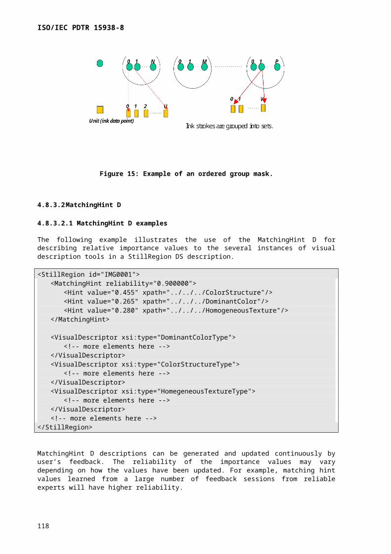
ISO/IEC PDTR 15938-8
4.8.4.9.2 MovingRegion DS extraction
Moving regions can be the result of spatio-temporal segmentation methods. This may be done automatically or by hand, based on semantics or other criteria. . An overview of spatio-temporal segmentation can be found in . This subclause describes the semi-automatic method used in the AMOS system to segment and track semantic objects in video sequences.
AMOS is a system that combines low level automatic region segmentation with an active method for defining and tracking high-level semantic video objects. A semantic object is represented as a set of underlying homogeneous regions. The system considers two stages (see Figure 28): an initial object segmentation stage where user input in the starting frame is used to create a semantic object, and an object tracking stage where underlying regions of the semantic object are automatically tracked and grouped through successive frames.1
Object Definition (user input)
Region Segmentation
Region Tracking
Motion Projection
Homogeneous Regions
Region Aggregation
Video Objects
starting frame
succeeding frame
2
Figure 28: General Structure of AMOS.
4.8.4.9.2.1 Initial Semantic Object Segmentation
Semantic object segmentation at the starting frame consists of several major processes as shown in Figure 29. First, users identify a semantic object by using tracing interfaces (e.g. mouse). The input is a polygon whose vertices and edges are roughly along the desired object boundary. To tolerate user-input error, a snake algorithm may be used to align the user-specified polygon to the actual object boundary. The snake algorithm is based on minimizing a specific energy function associated with edge pixels. Users may also choose to skip the snake module if a relatively accurate outline is already provided.
After the object definition, users can start the tracking process by specifying a set of thresholds. These thresholds include a color merging threshold, weights on three color channels (i.e. L*u*v*), a motion merging threshold and a tracking buffer size (see following subclauses for their usage). These thresholds can be chosen based on the characteristic of a given video shot and experimental results. For example, for a video shot where foreground objects and background regions have similar luminance, users may choose a lower weight on the luminance channel. Users can start the tracking process for a few frames with the default thresholds, which are automatically generated by the system, and then adjust the thresholds based on the segmentation and tracking results. This system also allows a user to stop the tracking process at any frame, modify the object boundary that is being tracked and then restart the tracking process from the modified frame.
120

ISO/IEC PDTR 15938-8
Figure 29: Object segmentation at starting frame.
Given the initial object boundary from users (or the snake module), a slightly extended (~15 pixels) bounding box surrounding the arbitrarily shaped object is computed. Within the bounding box, three feature maps, edge map, color map, and motion field, are created from the original images. Color map is the major feature map in the following segmentation module. It is generated by first converting the original image into the CIE L*u*v* color space and then quantizing pixels to a limited number of colors (e.g. 32 or 16 bins) using a clustering based (e.g. K-Means) method. The edge map is a binary mask where edge pixels are set to 1 and non-edge-pixels are set to 0. It is generated by applying the Canny edge detection algorithm. The motion field is generated by a hierarchical block matching algorithm . A 3-level hierarchy is used as suggested in .
The spatial intra-frame segmentation module is based on an automatic region segmentation algorithm using color and edge information ,. As stated in ,, color-based region segmentation can be greatly improved by fusion with edge information. Color based region merging works well on quantized and smoothed images. On the contrary, edge detection captures high-frequency details in an image. In AMOS, to further improve the accuracy, a motion-based segmentation process using the optical flow is applied to segmented color regions to check the uniformity of the motion distribution. Although the complete process utilizing color, edge, and motion is not trivial, the computational complexity is greatly reduced by applying the above region segmentation process only inside the bounding box of the snake object instead of the whole frame.
The region aggregation module takes homogeneous regions from the segmentation and the initial object boundary from the snake (or user input directly). Aggregation at the starting frame is relatively simple compared with that for the subsequent frames, as all regions are newly generated (not tracked) and the initial outline is usually not far from the real object boundary. A region is classified as foreground if more than a certain percentage (e.g. 90%) of the region is included in the initial object. On the other hand, if less than a certain percentage (e.g. 30%) of a region is covered, it is considered as background. Regions between the low and high thresholds are split into foreground and background regions according to the intersection with the initial object mask.
Finally, Affine motion parameters of all regions, including both foreground and background, are estimated by a multivariate linear regression process over the dense optical flow inside each region. In our system, a 2-D Affine model with 6 parameters is used. These Affine models will be used to help track the regions and object in the future frames, as will be discussed in the next subclause.
4.8.4.9.2.2 Semantic Object Tracking
Given the object with homogeneous regions constructed at the starting frame, tracking in the successive frames is achieved by motion projection and an inter-frame segmentation process. The main objectives of the tracking process are to avoid losing foreground regions and to avoid including false background regions. It contains the following steps (see Figure 30).
121

ISO/IEC PDTR 15938-8
Figure 30: Automatic semantic object tracking.
First, segmented regions from the previous frame, including both foreground and background, are projected onto the current frame (virtually) using their individual Affine motion models. Projected regions keep their labels and original classifications. For video shots with static or homogeneous background (i.e. only one moving object), users can choose not to project the background regions to save time.
Generation of the three feature maps (color, edge and motion) utilizes the same methods as described in the previous subclause. The only difference is that in the quantization step, the existing color palette computed at the starting frame is directly used to quantize the current frame. Using a consistent quantization palette enhances the color consistency of segmented regions between successive frames, and thus improves the performance of region based tracking. As object tracking is limited to single video shots, in which there is no abrupt scene change, using one color palette is generally valid. Certainly, a new quantization palette can be generated automatically when a large quantization error is found.
In the tracking module (i.e. inter-frame segmentation), regions are classified into foreground, background and new regions. Foreground or background regions tracked from the previous frame are allowed to be merged with regions of the same class, but merging across different classes is forbidden. New regions can be merged with each other or merged with foreground/background regions. When a new region is merged with a tracked region, the merging result inherits its label and classification from the tracked region. In motion segmentation, split regions remain in their original classes. After this inter-frame tracking process, a list of regions temporarily tagged as either foreground, background, or new is obtained. They are then passed to an iterative region aggregation process.
The region aggregation module takes two inputs: the homogeneous region and the estimated object boundary. The object boundary is estimated from projected foreground regions. Foreground regions from the previous frame are projected independently and the combination of projected regions forms the mask of the estimated object. The mask is refined with a morphological closing operation (i.e. dilation followed by erosion) with a size of several pixels in order to close tiny holes and smooth boundaries. To tolerate motion estimation error that may cause the loss of foreground regions around object boundary, the mask is further dilated with the tracking buffer size, which is specified by users at the beginning of the tracking.
The region aggregation module implements a region grouping and boundary alignment algorithm based on the estimated object boundary as well as the edge and motion features of the region. Background regions are first excluded from the semantic object. For every foreground or new region, intersection ratio of the region with the object mask is computed. Then if:
1) the region is foreground
If it is covered by the object mask by more than 80%, it belongs to the semantic object. Otherwise, the region is intersected with the object mask and split :
122

ISO/IEC PDTR 15938-8
a) split regions inside the object mask are kept as foreground
b) split regions outside the object mask are tagged as new
2) the region is new
If it is covered by the object mask by less than 30%, keep it as new; else if the region is covered by the object mask by more than 80%, classify it as foreground.
Otherwise:
a) Compute the numbers of edge pixels (using the edge map) between this region and the current background and foreground regions. Compute the differences between the mean motion vector of this region with those of its neighboring regions and find the neighbor with the most similar motion.
b) If the region is separated from background regions by more edge pixels than foreground regions (or if this region is not connected to any background regions) and its closest motion neighbor is a foreground region, intersect it with the object mask and split :
- split regions inside the object mask are classified as foreground
- split regions outside the object mask are tagged as new
c) Otherwise, keep the region as new.
Compared with the aggregation process in the previous subclause, a relatively lower ratio (80%) is used to include a foreground or new region. This is to handle motion projection errors. As it is possible to have multiple layers of new regions emerging between the foreground and the background, the above aggregation and boundary alignment process is iterated multiple times. This step is useful in correcting errors caused by rapid motions. At the end of the last iteration, all remaining new regions are classified into background regions. Finally, Affine models of all regions, including both foreground and background, are estimated. As described before, these Affine models are used to project regions onto the future frame in the motion projection module.
4.8.4.9.3 MovingRegion DS use
Moving region descriptions can be used for retrieval, browsing, and visualization applications. This subclause describes a query model for similarity searching of video objects based on localized visual features of the objects and the objects’ regions, and spatio-temporal relations among the objects’ regions . In moving region descriptions, the video objects will correspond to the first level of moving regions (InterviewerMR in MovingRegion DS on Informative Examples subclause of the MovingRegion DS of the MDS CD); the objects’ regions to the second level of moving regions (MR1 and MR2 MovingRegion DS on the Informative Examples of the MovingRegion DS of the MDS CD); the visual features to visual descriptors; and the spatio-temporal relations to segment relations in segment graphs.
Each video object has a unique ObjectID. Similarly each region also has a unique RegionID. Several visual descriptors (e.g. GoFColor) are associated with ObjectID and RegionID. In addition, ObjectID is associated with spatio-temporal descriptors as described on the Extraction subclause of the MovingRegion DS. These ID’s are used as indexes in the description of the object matching and retrieval processes described below.
Given a query object with N regions, the searching approach in consists of two stages:
(1) Region Search: to find a candidate region list for each query region based on visual features and spatio-temporal relations
(2) Joint & Validation: to join these candidate region lists to produce the best matched video objects by combining visual and structure similarity metrics and to compute the final global distance measure.
123

ISO/IEC PDTR 15938-8
The video object query model is shown in Figure 31.
Region Matching :for each query region, find candidate region list based on visual feature distance (i.e. color, texture, etc)
Join & Validation :join candidate region lists and compute total object distance (visual features + spatio-temporal relations)
Query Object
Retrieved Objects
Figure 31: The video object query model.
The detailed procedure follows:
1) For every query region, find a candidate region list based on the weighted sum (according to the weights given by users) of distance measures of different visual features (e.g., shape or trajectory). All individual feature distances are normalized to [0,1]. Only regions with distances smaller than a threshold are added to a candidate list. Here the threshold is a pre-set value used to empirically control the number or percentage of objects that the query system will return. For example, a threshold 0.3 indicates that users want to retrieve around 30 percent of video objects in the database (assuming the descriptors of the video objects in the database have normal distribution in feature spaces). The threshold can be set to a large value to ensure completeness, or a small value to improve speed.
2) Sort regions in each candidate region list by their ObjectID’s.
3) Perform join (outer join) of the region lists on ObjectID to create a candidate object list. Each candidate object, in turn, contains a list of regions. A "NULL" region is used when: (1) a region list does not contain regions with the ObjectID of a being-joined object and (2) a region appears (i.e. matched) more than once in a being-joined object.
4) Compute the distance between the query object and each object in the candidate object list as follows:
D = w 0 FD (q i, r i) + w 1 SD (sog q, sog o) +
w 2 SD (topo q, topo o) +w 3 SD (temp q, temp o)
where q i is the ith query region. r i is the ith region in a candidate object. FD(.) is the feature distance between a region and its corresponding query region. If r i is NULL, maximum distance (i.e., 1) is assigned. sog q (spatial orientation), topo q (topological relation) and temp q (temporal relation) are structure features of the query object sog o, topo o, and temp o are retrieved from database based on ObjectID, RegionID and temporal positions. When there is a NULL region (due to the above join process), the corresponding dimension of the retrieved descriptorwill have a NULL value. SD(.) is the L1-distance and a penalty of maximum difference is assigned to any dimension with a NULL value.
Sort the candidate object list according to the above distance measure D and return the result.
124

ISO/IEC PDTR 15938-8
4.8.4.10 Moving region decomposition tools
4.8.4.10.1 Moving region decomposition tools examples
The following example illustrates the use of the MovingRegionTemporalDecomposition DS for describing a video object plane or key still region of the moving region id = "ManMR" in 4.8.3.1.4.1. In this example, the still region id = "ManKeySR" represents the still region of the object "Man" in a video frame. The segment decomposition has gaps but no overlaps. The spatial localization of the still region id = "ManKeySR" is described using the SpatialLocator datatype.
<Mpeg7><Description xsi:type="ContentEntityType">
<MultimediaContent xsi:type="VideoType"><Video id="VS1">
<SpatioTemporalDecomposition><MovingRegion id="ManMR">
<TextAnnotation><FreeTextAnnotation> Man (moving
region)</FreeTextAnnotation></TextAnnotation><TemporalDecomposition gap="true" overlap="false">
<StillRegion id="ManKeySR"><MediaLocator>
<MediaUri>image.jpg</MediaUri></MediaLocator><TextAnnotation>
<FreeTextAnnotation> Man (still region)</FreeTextAnnotation>
</TextAnnotation><VisualDescriptor xsi:type="ScalableColorType"
numOfCoeff="16" numOfBitplanesDiscarded="0"><Coeff> 1 2 3 4 5 6 7 8 9 0 1 2 3 4 5 6
</Coeff></VisualDescriptor>
</StillRegion></TemporalDecomposition>
</MovingRegion></SpatioTemporalDecomposition>
</Video></MultimediaContent>
</Description></Mpeg7>
4.8.4.11 VideoText DS
4.8.4.11.1 VideoText DS examples
The following example illustrates the use of the VideoText DS for describing a superimposed video text with text string "Victory".
<Mpeg7><Description xsi:type="ContentEntityType">
<MultimediaContent xsi:type="VideoType"><Video id="VS1">
<SpatioTemporalDecomposition><MovingRegion xsi:type="VideoTextType" id="VideoText1"
textType="superimposed" fontSize="40" fontType="Courier New">
<Text> Victory </Text>
125

ISO/IEC PDTR 15938-8
</MovingRegion></SpatioTemporalDecomposition>
</Video></MultimediaContent>
</Description></Mpeg7>
4.8.4.11.2 VideoText DS extraction
Extraction of videotext in a frame is the result of image analysis involving text character segmentation and location. This may be done automatically or by hand, based on semantics or other criteria. This subclause discusses how videotext can be extracted automatically from digital videos. Text can appear in a video anywhere in the frame and in different contexts. The algorithms presented here are designed to extract superimposed text and scene text, which possesses typical (superimposed) text attributes. No prior knowledge about frame resolution, text location, font styles, and text appearance modes such as normal and inverse video are assumed. Some common characteristics of text are exploited in the algorithms including monochromaticity of individual characters, size restrictions (characters cannot be too small to be read by humans or too big to occupy a large portion of the frame), and horizontal alignment of text (preferred for ease of reading).
Approaches to extracting text from videos can be broadly classified into three categories: (i) methods that use region analysis, (ii) methods that perform edge analysis, and (iii) methods that use texture information. The following subclause describes a region-based algorithm , which is followed by a subclause containing an edge-based algorithm .
4.8.4.11.2.1 Videotext Extraction Using Region Analysis
The region analysis algorithm for videotext extraction works by extracting and analyzing regions in a video frame. The goals of this system are (i) isolating regions that may contain text characters, (ii) separating each character region from its surroundings and (iii) verifying the presence of text by consistency analysis across multiple text blocks.
4.8.4.11.2.1.1 Candidate Text Region Extraction
The first step in the region analysis system is to remove non-text background from an input gray scale image generated by scanning a paper document, or from downloading a Web image, or by decompressing an encoded (for example, in MPEG-1, 2) video stream. The generalized region labeling (GRL) algorithm is used to extract homogenous regions from this image. The GRL algorithm labels pixels in an image based on a given criterion (e.g., gray scale homogeneity) using contour traversal, thus partitioning the image into multiple regions, then groups pixels belonging to a region by determining its interior and boundaries, and extracts region features such as its MBR (minimum bounding rectangle), area, etc. The criterion used to group pixels into regions is that the gray level difference between any pair of pixels within the region cannot exceed ±10.
The GRL algorithm thus, segments the image into nonoverlapping homogenous regions. It also results in complete region information such as its label, outer and inner boundaries, number of holes within the regions, area, average gray level, gray level variance, centroid and the MBR. Next, non-text background regions among the detected regions are removed based on their size. A region is removed if the width and height of its MBR are greater than 24 and 32, respectively (can be adaptively modified depending on the image size). By employing a spatial proportion constraint, rather than area constraint, large homogeneous regions which are unlikely to be text are removed. Within the remaining candidate regions, candidate regions may be fragmented into multiple regions because of varying contrast in the regions surrounding the candidate regions. To group multiple touching regions into a single coherent region, a binary image from the labeled region image where all the regions which do not satisfy the size constraint are marked "0" and the remaining regions are marked "1" is generated. This binary image is processed using the GRL algorithm to obtain new connected regions. With the creation of a binary image, followed by a relabeling step, many small connected fragments of a candidate text region are merged together.
126

ISO/IEC PDTR 15938-8
4.8.4.11.2.1.2 Text Region Refinement
Here the basic idea is to apply appropriate criteria to extract character segments within the candidate regions. Within a region, characters with holes can be present embedded in a complex background and since OCR systems require text to be printed against a clean background for processing, the second stage attempts to remove the background within the regions while preserving the candidate character outline. Since character outlines in these regions can be degraded and merged with the background, an iterative local thresholding operation is performed in each candidate region to separate the region from its surroundings and from other extraneous background contained within its interior. Once thresholds are determined automatically for all candidate regions, positive and negative images are computed. The positive image contains region pixels whose gray levels are above their respective local thresholds and the negative image contains region pixels whose gray levels fall below their respective thresholds. Observe that the negative image will contain candidate text regions if that text appears in inverse video mode. All the remaining processing steps are performed on both positive and negative images and their results are combined. Thus the region analysis system can handle normal and inverse video appearances of text.
The character region boundaries are further sharpened and separated by performing a region boundary analysis. This is necessary especially when characters within a text string appear connected with each other and they need to be separated for accurate text identification. This is achieved by examining the gray level contrast between the character region boundaries and the regions themselves. For each candidate region R, a threshold T is computed:
where Icbk is the gray level of the pixel k on the circumscribing boundaries of the region and I il is the gray level of the pixel l belonging to R (including interior and region boundary), Ncb is the number of pixels on the circumscribing boundaries of the region, and N i is the number of pixels in the region. A pixel is defined to be on the circumscribing boundary of a region if it does not belong to the region but at least one of its four neighbors (using 4-connectivity) does. Those pixels in R whose gray level is less than T are marked as belonging to the background and discarded, while the others are retained in the region. Note that this condition is reversed for the negative image. This step is repeated until the value of T does not change over two consecutive iterations.
4.8.4.11.2.1.3 Text Characteristics Verification
The few candidate character regions are now tested for exhibiting typical text font characteristics. A candidate region is removed if its area is less than 12 or its height is less than 4 pixels because small fonts are difficult to be recognized by OCR systems. It is also removed if the ratio of the area of its MBR to the region area (fill factor) is greater than 4. Finally it may be removed if the gray level contrast with the background is low, i.e., if
where Icbk is the gray level of the pixel k on the circumscribing boundaries of the region and I bl is the gray level of the pixel l on the boundaries of the region. Since region boundary information is easily available owing to our GRL algorithm, this new boundary-based test can be easily performed to handle the removal of noisy non-text regions. Note also that the parameters used were determined with a study of a large number of SIF-resolution videos and were kept stable during our experimentation.
4.8.4.11.2.1.4 Text Consistency Analysis
Consistency between neighboring text regions is verified to eliminate false positive regions. The system attempts to ensure that the adjacent regions in a line exhibit the characteristics of a text string, thus locally verifying the global structure of the line. This text consistency test includes:
1. position analysis that checks inter-region spacing. The width between the centroids of the MBRs of a pair of neighboring regions that are retained is less than 50 pixels;
127

ISO/IEC PDTR 15938-8
2. horizontal alignment analysis of regions. The vertical centers of neighboring MBRs is within 6 pixels of one another;
3. vertical proportions analysis of adjacent regions. The height of the larger of the two regions is less than twice the height of the smaller region.
Given a candidate text string, a final series of tests involving their MBRs are also performed. The MBRs of the regions (characters) are first verified to be present along a line within a given tolerance of 2 pixels. Observe that characters present along a diagonal line can be therefore easily identified as a string in the region analysis system. The inter-region distance in the string is verified to be less than 16 pixel. The MBRs of adjacent regions are ensured not to overlap by more than 2 pixels. If all three conditions are satisfied, the candidate word region is retained as a text string. The final output is a clean binary image containing only the detected text characters (appearing as black on white background) that can be directly used as input to an OCR system in order to be recognized.
4.8.4.11.2.1.5 Interframe Analysis For Text Refinement
Optionally, if consecutive frames in videos are being processed together in a batch job, then text regions determined from say, five consecutive frames can be analyzed together to add missing characters in frames and to delete incorrect regions posing as text. This interframe analysis used by the region analysis system to handle videos exploits the temporal persistence of videotext, and it involves examination of the similarity of text regions in terms of their positions, intensities and shape features and aids in omitting false positive regions.
4.8.4.11.2.2 Text Detection Based on Edge Characterization
The edge characterization algorithm for text detection exploits the text properties namely, the height, width and area on the connected components (CC) of the edges detected in frames. Furthermore, horizontal alignment is used to merge multiple CC's into a single line of text. The purpose is to output a thresholded image of the detected text lines with text as foreground in black on a white background. This can be the input to an OCR to recognize the text characters.
Text extraction is performed on individual video frames. The steps involved in text extraction are given below. The origin (0,0) of the frame is the top-left corner. Any pixel is referenced by (x, y) location where x, is the position in columns and y, in rows.
4.8.4.11.2.2.1 Channel Separation
The red frame of the RGB color space is used to make it easy to differentiate the colors white, yellow and black, which dominate videotext. By using the red frame, sharp high-contrast edges for these frequent text colors are obtained. However, other color spaces such as HSB or YUV could be used.
4.8.4.11.2.2.2 Image Enhancement
The frame’s edges are enhanced using a 3 ´ 3-mask. Noise is further removed using a median filter.
4.8.4.11.2.2.3 Edge Detection
On the enhanced image, edge detection is performed using the following 3 ´ 3 filter.
-1 -1 -1
-1 12 -1
-1 -1 -1
128

ISO/IEC PDTR 15938-8
Excluding the image borders, edges are found when the output is smaller than EdgeThreshold. Currently, the threshold is fixed; however, a variable threshold could be used. The fixed threshold results in a lot of salt and pepper noise; also, the edges around the text may be broken and not connected. Hence, further processing is needed.
4.8.4.11.2.2.4 Edge Filtering
A preliminary edge filtering is performed to remove areas that possibly do not contain text or, even if they do, they cannot be reliably detected. Edge filtering can be performed at different levels. One is at a frame level and the other is at a sub-frame level. On the frame level, if more than a reasonable portion of the frame contains edge pixels, probably due to the number of scene objects, the frame is disregarded and the next one is taken. This can lead to the loss of text in some clean areas and result in false negatives. To overcome this problem, edge filtering is performed at a sub-frame level. To find text in an "over croCDed" frame, six counters are maintained with the count of the subdivided frame. Three counters are used for three vertical portions of the frame (one third of the area of the frame). Similarly, three counters are used for three horizontal stripes. Text lines found in high-density edge areas (stripes) are rejected in a subsequent step. This filtering could be done using smaller areas, to retain areas that are clean and contain text in a region smaller than one-third of an image.
4.8.4.11.2.2.5 Character Detection
Next a Connected Component (CC) analysis is performed on leftover edges. Text characters are assumed to give rise to connected components or a part thereof. All the edge pixels that are located within a certain distance from each other (an eight-pixel neighborhood is used) are merged in CCs. Each of the CCs is tested for size, height, width and area criteria before passing to the next stage.
4.8.4.11.2.2.6 Text Box Detection
The connected components that pass the criteria in the previous step are sorted in ascending order based on the location of the bottom left pixel. The sorting is done in raster scan. This list is traversed and the CCs are merged together to form boxes of text. The first connected component, CC1 is assigned to the first box. Each subsequent CC i is tested to see if the bottom most pixel lies within a preset acceptable "row" threshold from the bottom most pixel of the current text box. If the CC i lies within a few rows (in this case 2 rows) of the current box, there is a good chance that they belong to the same line of text. The row difference threshold currently used, is a fixed one, but a variable one could also be used. It could be made a fraction of the height of the current text box. In order to avoid merging CCs that are too far away in the image, a second test is performed to see if the column distance between CCi and the text boxes is less than a column threshold. This threshold is variable and is a multiple of the width of CCi. CCi is merged to the current text box if the above is true. If CC i
does not merge into the current text box, then a new text box is started with CC i as its first component and the traversing is continued.
The above process could result in multiple text boxes for a single line of text in the image. Now for each of the text boxes formed by the character merging, a second level of merging is performed. This is to merge the text boxes that might have been mistakenly taken as separate lines of text, either due to strict CC merging criteria or due to poor edge detection process resulting in multiple CCs for the same character.
Each box is compared to the text boxes following it for a set of conditions. If two boxes are merged, the second box is deleted from the list of text boxes and merged into the first box. The multiple test conditions for two text boxes are:
1. The bottom of one box is within the row difference threshold of the other. Also the distance between the two boxes in the horizontal direction is less than a variable threshold depending on the average width of characters in the first box.
2. The center of either of the boxes lies within the area of the other text box
3. The text boxes overlap.
129

ISO/IEC PDTR 15938-8
If any of the above conditions is satisfied, the two text boxes are merged until all text boxes are tested against each other.
4.8.4.11.2.2.7 Text Line Detection and Enhancement
The leftover boxes are accepted as text lines if they conform to the constraints of area, width and height. For each of the boxes, the corresponding original sub-image is thresholded to obtain the text as foreground in black and everything else in white. This is required so that the binary image can be inputted to an OCR. The average grayscale value of the pixels in the box is calculated. The average grayscale, AvgBG, value of a region (5 pixels in our case) around the box is calculated. Within the box, anything above the average is marked as white and anything below it is marked as black. The grayscale average for the pixels being marked as white, Avg1, is calculated along the average of the black pixels, Avg2. Once, the box is converted to a black and white image (binary image), the average of the "white region"(Avg1) and the average of the "black region"(Avg2) are compared to the AvgBG (as shown in Figure 32). The region that has its average closer to the AvgBG is assigned to be the background and the other region is assigned to be the foreground. In other words, if the "black region" has its average closer to the other average, it is converted to white and vice versa. This assures that the text is always in black.
1.1.1.1.1.1.1Avg1Avg2
5 pixels
Figure 32: Separation of text foreground from background.
4.8.4.11.3 VideoText DS use
The applications described here highlight video browsing scenarios in which interesting events (i.e., the presence of videotext as an indicator of information pertaining to persons, locations, product advertisements, sports scores, etc) in the video are detected automatically and the video content is browsed based on these events, and video classification scenarios.
The application with an event-based video browsing capability shows that frames containing videotext can be automatically determined from a digital video stream. The stream can be marked as those segments containing videotext and those who do not by automatically determining the contiguous groups of time intervals of frames that contain text and which do not. Consequently, the video can be browsed in a nonlinear and random-access fashion based on the occurrence of a specific event. The event in this case is the presence or absence of videotext. A graphical summary of the video shows where videotext annotation is present along the video timeline.
With an application demonstrating video classification, the use of videotext in conjunction with other video features (annotations) for classification can be shown. Videotext annotation in news programs along with the detection of talking heads results in automatically labeled anchor shots.
4.8.5 Audio segment description tools
4.8.5.1 AudioSegment DS
4.8.5.1.1 AudioSegment DS examples
The following examples illustrate the use of the AudioSegment DS for describing audio content. The MediaTime describes the time information for the audio segment.
<AudioSegment><MediaTime>
<MediaTimePoint>T00:00:00</MediaTimePoint><MediaDuration>PT1M30S</MediaDuration>
</MediaTime>
130
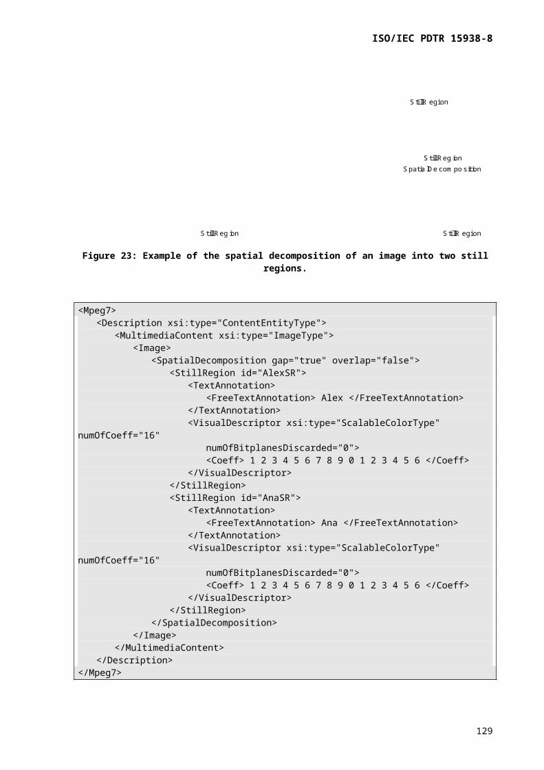
ISO/IEC PDTR 15938-8
</AudioSegment>
4.8.5.2 Audio segment decomposition tools
4.8.5.2.1 Audio segment decomposition tools examples
The following example illustrates the use of the AudioSegmentTemporalDecomposition DS for describing the temporal decomposition of audio content.
<Mpeg7><Description xsi:type="ContentEntityType">
<MultimediaContent xsi:type="AudioType"><Audio>
<MediaTime><MediaTimePoint>T00:00:00</MediaTimePoint><MediaDuration>PT1M30S</MediaDuration>
</MediaTime><TemporalDecomposition gap="false" overlap="false">
<AudioSegment><TextAnnotation>
<FreeTextAnnotation> Chase </FreeTextAnnotation></TextAnnotation><MediaTime>
<MediaTimePoint>T00:00:00</MediaTimePoint><MediaDuration>PT0M15S</MediaDuration>
</MediaTime></AudioSegment><AudioSegment>
<TextAnnotation><FreeTextAnnotation> Capture </FreeTextAnnotation>
</TextAnnotation><MediaTime>
<MediaTimePoint>T00:00:15</MediaTimePoint><MediaDuration>PT1M15S</MediaDuration>
</MediaTime></AudioSegment>
</TemporalDecomposition></Audio>
</MultimediaContent></Description>
</Mpeg7>
4.8.6 Audio-visual segment description tools
4.8.6.1 AudioVisualSegment DS
4.8.6.1.1 AudioVisualSegment DS examples
The following example illustrates the use of the AudioVisualSegment DS for describing an AV segment.
<AudioVisualSegment id="DocumentaryAVS"><MediaLocator>
<MediaUri>movie.mpg</MediaUri></MediaLocator><TextAnnotation>
<FreeTextAnnotation> Documentary about eagles </FreeTextAnnotation>
131

ISO/IEC PDTR 15938-8
</TextAnnotation><MediaTime>
<MediaTimePoint>T00:00:00</MediaTimePoint><MediaDuration>PT1M30S</MediaDuration>
</MediaTime></AudioVisualSegment>
4.8.6.2 Audio-visual segment decomposition tools
4.8.6.2.1 Audio-visual segment decomposition tools examples
The following example illustrates the use of the AudioVisualSegmentMediaSourceDecomposition DS in the AudioVisualSegment DS for describing the audio and video constituents of the AV segment "EagleDocumentaryAVS" in 4.8.6.1.1. In this example, the AV segment "EagleDocumentaryAVS" represents the full video sequence that is decomposed into one audio segment, "EagleDocumentaryAS" and one video segment, "EagleDocumentaryVS", corresponding to the audio and video tracks, respectively. Each segment is connected in space and/or time, as applicable.
<Mpeg7><Description xsi:type="ContentEntityType">
<MultimediaContent xsi:type="AudioVisualType"><AudioVisual>
<MediaLocator><MediaUri>movie.mpg</MediaUri>
</MediaLocator><TextAnnotation>
<FreeTextAnnotation> Eagle Documentary </FreeTextAnnotation>
</TextAnnotation><MediaTime>
<MediaTimePoint>T00:00:00</MediaTimePoint><MediaDuration>PT1M30S</MediaDuration>
</MediaTime><TemporalDecomposition>
<AudioVisualSegment id="EagleDocumentaryAVS"><TextAnnotation>
<FreeTextAnnotation> Eagle Documentary </FreeTextAnnotation>
</TextAnnotation><MediaTime>
<MediaTimePoint>T00:00:00</MediaTimePoint><MediaDuration>PT1M30S</MediaDuration>
</MediaTime><MediaSourceDecomposition gap="false" overlap="false">
<VideoSegment id="EagleDocumentaryVS"><MediaTime>
<MediaTimePoint>T00:00:00</MediaTimePoint><MediaDuration>PT1M30S</MediaDuration>
</MediaTime><VisualDescriptor xsi:type="GoFGoPColorType"
aggregation="Average"><ScalableColor numOfCoeff="16"
numOfBitplanesDiscarded="0"><Coeff> 1 2 3 4 5 6 7 8 9 0 1 2 3 4 5 6
</Coeff></ScalableColor>
</VisualDescriptor></VideoSegment>
132

ISO/IEC PDTR 15938-8
<AudioSegment id="EagleDocumentaryAS"><MediaTime>
<MediaTimePoint>T00:00:00</MediaTimePoint><MediaDuration>PT1M30S</MediaDuration>
</MediaTime></AudioSegment>
</MediaSourceDecomposition></AudioVisualSegment>
</TemporalDecomposition></AudioVisual>
</MultimediaContent></Description>
</Mpeg7>
4.8.6.3 AudioVisualRegion DS
4.8.6.3.1 AudioVisualRegion DS examples
The following example illustrates the use of the AudioVisualRegion DS for describing an AV Region. In this example, the AV region id = "NarratorAVR" represents the spatio-temporal region of the video and the temporal segment of the audio corresponding to the object "Narrator". The VisualSpatioTemporalLocator and the AudioMediaTime locate the AV region in the video and the audio, respectively.
<Mpeg7><Description xsi:type="ContentEntityType">
<MultimediaContent xsi:type="AudioVisualType"><AudioVisual>
<MediaLocator><MediaUri>movie.mpg</MediaUri>
</MediaLocator><TextAnnotation>
<FreeTextAnnotation> Eagle Documentary </FreeTextAnnotation>
</TextAnnotation><MediaTime>
<MediaTimePoint>T00:00:00</MediaTimePoint><MediaDuration>PT1M30S</MediaDuration>
</MediaTime><SpatioTemporalDecomposition>
<AudioVisualRegion id="NarratorAVR"><TextAnnotation>
<FreeTextAnnotation> Video and audio of narrator </FreeTextAnnotation>
</TextAnnotation><VisualSpatioTemporalLocator>
<FigureTrajectory type="rectangle"><MediaTime>
<MediaTimePoint>T00:00:15</MediaTimePoint><MediaDuration>PT1M15S</MediaDuration>
</MediaTime><Vertex>
<WholeInterval><MediaDuration>PT0S</MediaDuration>
</WholeInterval><InterpolationFunctions>
<KeyValue type="startPoint"><!-- more elements here -->
</KeyValue>
133

ISO/IEC PDTR 15938-8
<KeyValue type="startPoint"><!-- more elements here -->
</KeyValue></InterpolationFunctions>
</Vertex><Vertex>
<WholeInterval><MediaDuration>PT1S</MediaDuration>
</WholeInterval><InterpolationFunctions>
<KeyValue type="startPoint"><!-- more elements here -->
</KeyValue><KeyValue type="startPoint">
<!-- more elements here --></KeyValue>
</InterpolationFunctions></Vertex><Vertex>
<WholeInterval><MediaDuration>PT2S</MediaDuration>
</WholeInterval><InterpolationFunctions>
<KeyValue type="startPoint"><!-- more elements here -->
</KeyValue><KeyValue type="startPoint">
<!-- more elements here --></KeyValue>
</InterpolationFunctions></Vertex><!-- more elements here -->
</FigureTrajectory></VisualSpatioTemporalLocator><AudioMediaTime>
<MediaTimePoint>T00:00:00</MediaTimePoint><MediaDuration>PT1M30S</MediaDuration>
</AudioMediaTime></AudioVisualRegion>
</SpatioTemporalDecomposition></AudioVisual>
</MultimediaContent></Description>
</Mpeg7>
4.8.6.4 Audio-visual region decomposition tools
4.8.6.4.1 Audio-visual region decomposition tools examples
The following example illustrates the use of the AudioVisualRegionMediaSourceDecomposition DS in the AudioVisualRegion DS for describing the video and audio constituents of the AV region "NarratorAVR" in 4.8.6.3.1. In this example, the AV region "NarratorAVR" is decomposed into the moving region "NarratorMR" and the audio segment "Narrator AS" corresponding to the video and audio data of the object "Narrator", respectively. Each segment is connected in space and/or time, as applicable.
<Mpeg7><Description xsi:type="ContentEntityType">
<MultimediaContent xsi:type="AudioVisualType">
134

ISO/IEC PDTR 15938-8
<AudioVisual><MediaLocator>
<MediaUri>movie.mpg</MediaUri></MediaLocator><TextAnnotation>
<FreeTextAnnotation> Eagle Documentary </FreeTextAnnotation>
</TextAnnotation><MediaTime>
<MediaTimePoint>T00:00:00</MediaTimePoint><MediaDuration>PT1M30S</MediaDuration>
</MediaTime><SpatioTemporalDecomposition>
<AudioVisualRegion id="NarratorAVR"><TextAnnotation>
<FreeTextAnnotation> Video and audio of narrator </FreeTextAnnotation>
</TextAnnotation><MediaSourceDecomposition gap="false" overlap="false">
<MovingRegion id="NarratorMR"><TextAnnotation>
<FreeTextAnnotation> Moving region of narrator
</FreeTextAnnotation></TextAnnotation>
</MovingRegion><AudioSegment id="NarratorAS">
<MediaTime><MediaTimePoint>T00:00:00</MediaTimePoint><MediaDuration>PT01M30S</MediaDuration>
</MediaTime></AudioSegment>
</MediaSourceDecomposition></AudioVisualRegion>
</SpatioTemporalDecomposition></AudioVisual>
</MultimediaContent></Description>
</Mpeg7>
4.8.7 Multimedia segment description tools
4.8.7.1 MultimediaSegment DS
4.8.7.1.1 MultimediaSegment DS examples
The following examples illustrate the use of the MultimediaSegment DS for describing multimedia content.
<MultimediaSegment><TextAnnotation>
<FreeTextAnnotation> Multimedia content </FreeTextAnnotation></TextAnnotation>
</MultimediaSegment>
135

ISO/IEC PDTR 15938-8
4.8.7.2 Multimedia segment decomposition tools
4.8.7.2.1 Multimedia segment decomposition tools examples
The following examples illustrate the use of the MultimediaSegmentMediaSourceDecomposition DS for describing the decomposition of multimedia content into its video, audio, and image components.
<Mpeg7><Description xsi:type="ContentEntityType">
<MultimediaContent xsi:type="MultimediaType"><Multimedia>
<MediaSourceDecomposition gap="false" overlap="false"><Segment xsi:type="VideoSegmentType">
<TextAnnotation><FreeTextAnnotation> Chase video
</FreeTextAnnotation></TextAnnotation><MediaTime>
<MediaTimePoint>T00:00:00</MediaTimePoint><MediaDuration>PT0M15S</MediaDuration>
</MediaTime><VisualDescriptor xsi:type="GoFGoPColorType"
aggregation="Average"><ScalableColor numOfCoeff="16"
numOfBitplanesDiscarded="0"><Coeff> 1 2 3 4 5 6 7 8 9 0 1 2 3 4 5 6 </Coeff>
</ScalableColor></VisualDescriptor>
</Segment><Segment xsi:type="AudioSegmentType">
<TextAnnotation><FreeTextAnnotation> Chase audio
</FreeTextAnnotation></TextAnnotation>
</Segment><Segment xsi:type="StillRegionType">
<TextAnnotation><FreeTextAnnotation> Chase image
</FreeTextAnnotation></TextAnnotation>
</Segment></MediaSourceDecomposition>
</Multimedia></MultimediaContent>
</Description></Mpeg7>
4.8.8 Ink segment description tools
4.8.8.1 InkSegment DS
4.8.8.1.1 InkSegment DS examples
The following example illustrates the use of the InkSegment DS for describing the ink document, which consists of the word "Ana" surrounded by a circle keyword gesture. The strokes corresponding to the word "Ana" are a content ink segment; the strokes corresponding to the keyword gesture are a meta ink segment; finally, the full ink document is a mixed ink segment. In this example, the ink segments "ElecDoc1", "WordAna", and "KeywordGesture" represent the mixed ink segment, the
136

ISO/IEC PDTR 15938-8
content ink segment, and the meta ink segment, respectively. The ink segments "WordAna" and "KeywordGesture" are the result of the temporal decomposition of ink segment "ElecDoc1" because they have different temporal information.
In this example, the ink capture device records the temporal information of the ink data points with very low frequency so all the ink data points of ink segment "WordAna" carry the same temporal information and the ink segment "WordAna" can be spatially decomposed into ink segments that represent the different letters of the word, e.g., ink segment "LetterA".
<Mpeg7 xmlns="urn:mpeg:mpeg7:schema:2001" xmlns:mpeg7="urn:mpeg:mpeg7:schema:2001" xmlns:xsi="http://www.w3.org/2001/XMLSchema-instance" xsi:schemaLocation="urn:mpeg:mpeg7:schema:2001 .\mdsfdisver3.3.xsd">
<Description xsi:type="ContentEntityType"><MultimediaContent xsi:type="InkContentType">
<InkContent id="ElecDoc1" type="mixed"><MediaLocator>
<MediaUri>ink.mpg</MediaUri></MediaLocator><InkMediaInformation>
<InputDevice resolutionS="133"><Device>
<Name xml:lang="en">PenDevice</Name></Device>
</InputDevice><Handedness>right</Handedness><Style>mixed</Style>
</InkMediaInformation><TemporalDecomposition>
<InkSegment id="WordAna" type="content"><MediaTime>
<MediaRelTimePoint
mediaTimeBase="../../../../MediaLocator[1]">PT0S</MediaRelTimePoint><MediaDuration>PT3S</MediaDuration>
</MediaTime><HandWritingRecogResult>
<Quality>0.6</Quality><Result score="0.7">
<Text> Ana </Text></Result><Result score="0.54">
<Text> Ann </Text></Result>
</HandWritingRecogResult><SpatialDecomposition>
<InkSegment id="LetterA" type="content"><OrderedGroupDataSetMask>
<SubInterval setRef="#WordAna" startComponent="1731"
startUnit="36" endComponent="1742" endUnit="47"/>
</OrderedGroupDataSetMask><HandWritingRecogResult>
<Quality>0.4</Quality><Result score="0.54">
<Text> A </Text></Result>
</HandWritingRecogResult></InkSegment>
</SpatialDecomposition>
137
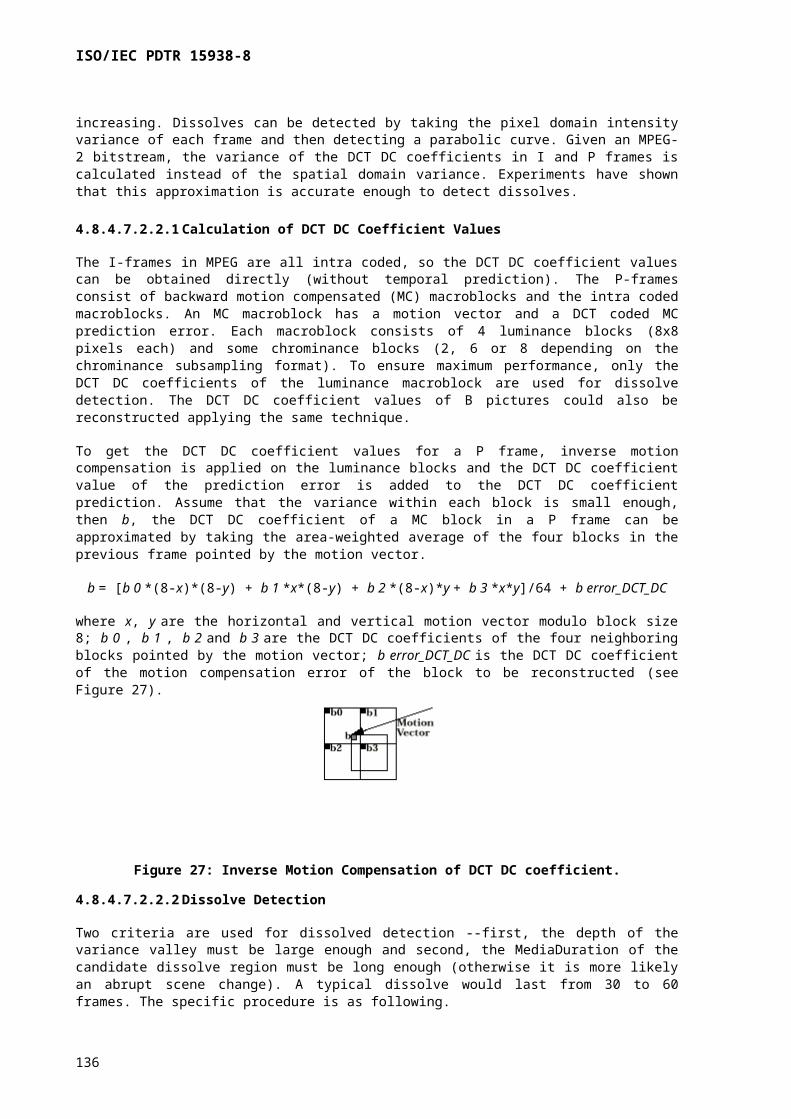
ISO/IEC PDTR 15938-8
</InkSegment><InkSegment id="KeywordGesture" type="meta">
<MediaTime><MediaRelTimePoint
mediaTimeBase="../../../../MediaLocator[1]">PT3S</MediaRelTimePoint><MediaDuration>PT2S</MediaDuration>
</MediaTime></InkSegment>
</TemporalDecomposition></InkContent>
</MultimediaContent></Description>
</Mpeg7>
The following example illustrates the use of the InkSegment DS to describe the ink document shown in Figure 33. The last four lines in Figure 33 are part of the ink data file and describe the structure of the ink data points in segments. For example, the third to last line describes a line in the ink data file that consists of the ink data points from stroke number 1699 point 43 to stroke number 1748 point 90 with the following recognized text "cause. In 1988 it was …".
Figure 33: Example of an ink document.
<Mpeg7><Description xsi:type="ContentEntityType">
<MultimediaContent xsi:type="InkContentType"><InkContent id="Paragraph-1">
<MediaLocator><MediaUri>http://www.mpeg7.org/demo.stk</MediaUri>
</MediaLocator><SpatialDecomposition gap="true" overlap="false">
138

ISO/IEC PDTR 15938-8
<InkSegment id="Line-7"><InkMediaInformation>
<InputDevice resolutionS="120"><Device>
<Name xml:lang="en">PenDevice</Name></Device>
</InputDevice></InkMediaInformation><OrderedGroupDataSetMask>
<SubInterval setRef="#Paragraph-1" startComponent="1699"
startUnit="43" endComponent="1748" endUnit="90"/>
</OrderedGroupDataSetMask><HandWritingRecogResult>
<Quality>0.9</Quality><Result score="1.0">
<Text> causes. In 1988 it was determined that the </Text>
</Result></HandWritingRecogResult><SpatialDecomposition gap="true" overlap="false">
<InkSegment id="WORD-6"><OrderedGroupDataSetMask>
<SubInterval setRef="#Paragraph-1" startComponent="1731" startUnit="36" endComponent="1742" endUnit="47"/>
</OrderedGroupDataSetMask><HandWritingRecogResult>
<Quality>0.9</Quality><Result score="1.0">
<Text> determined </Text></Result>
</HandWritingRecogResult></InkSegment>
</SpatialDecomposition></InkSegment>
</SpatialDecomposition></InkContent>
</MultimediaContent></Description>
</Mpeg7>
The following example illustrates the use of the StructuralUnit element in the InkSegment DS for describing the grouping of ink data points into pages, paragraph and commands, as defined by the creator. The root ink segment contains one content ink segment and one meta ink segment. The content ink segment is a page and is composed of two other content ink segments that are paragraphs. This example also illustrate the use of the Param element and the OverlaidMedia element in InkMediaInformation DS for describing the two parameters and the operand of the command, respectively. The command mails the ink segment "data" from [email protected] to [email protected].
<Mpeg7><Description xsi:type="ContentEntityType">
<MultimediaContent xsi:type="InkContentType"><InkContent type="mixed">
<TemporalDecomposition><InkSegment id="data" type="content">
<StructuralUnit href="urn:example:acs"><Name>Page</Name>
139

ISO/IEC PDTR 15938-8
</StructuralUnit><TemporalDecomposition>
<InkSegment><StructuralUnit href="urn:example:acs">
<Name>Paragraph</Name></StructuralUnit><MediaTime>
<MediaTimePoint>T00:00:00</MediaTimePoint><MediaDuration>PT1M30S</MediaDuration>
</MediaTime></InkSegment><InkSegment>
<StructuralUnit href="urn:example:acs"><Name>Paragraph</Name>
</StructuralUnit><MediaTime>
<MediaTimePoint>T00:01:30</MediaTimePoint><MediaDuration>PT1M04S</MediaDuration>
</MediaTime></InkSegment>
</TemporalDecomposition></InkSegment><InkSegment type="meta">
<StructuralUnit href="urn:example:acs"><Name>MAIL command</Name><Definition>
MAIL command is used to mail the content specified by theOverlaidMedia element in the InkMediaInformation DS.
There are twoAssociated parameterName "From" and "To". The associated parameterValues are to specify the sender
and receiver email address respectively.
</Definition></StructuralUnit><InkMediaInformation>
<OverlaidMedia><OverlaidMediaRef href="#data"/>
</OverlaidMedia><Param name="From" value="[email protected]"/><Param name="To" value="[email protected]"/>
</InkMediaInformation></InkSegment>
</TemporalDecomposition></InkContent>
</MultimediaContent></Description>
</Mpeg7>
An example scenario to show the usage of the InkSegment DS is the following. At the end of the ink content creation, ink content is captured into an ink data file, and the metastrokes are described as a meta ink segment. At the same time, the scene graph, the media space, and the ordered group dataset masks locate the ink strokes stored in the ink document. A hand-writing recognition engine, described using HandWritingRecogInformation DS, can make use of the ink media and creation information and/or the stroke data to recognize words in ink strokes. If it suceeds, it reports the results using the HandWritingRecogResult DS in the InkSegment DS. As a result, a text keyword search can be used. However, if the hand-writing recognition engine fails to recognize the ink strokes, the time sequences of meta ink segments can be used for matching. Although the masks are designed for the ink documents, they are general enough to be used for other media.
140

ISO/IEC PDTR 15938-8
4.8.8.2 InkMediaInformation DS
4.8.8.2.1 InkMediaInformation DS examples
The following example illustrates the use of the InkMediaInformation DS for describing the input device and handedness information for an ink segment.
<InkMediaInformation><InputDevice resolutionS="133">
<Device><Name xml:lang="en">PenDevice</Name>
</Device></InputDevice><Handedness>right</Handedness><Style>mixed</Style>
</InkMediaInformation>
The following example illustrates the use of the InkSegment DS and the OverlaidMedia element in the InkMediaInfo DS, among others, for describing ink content overlaying on a text medical form as shown in Figure 34. An example of application scenario for these kind of descriptions is the automatic collection of patient medical records for which the medical paper form stays on top of the writing surface of the ink input device. When the patient fills in the information on the paper form with a electronic pen, the information is simultaneously available as ink content.
In this example, the content ink segment is composed of three ink segments, each representing one word in the ink content. The WritingFieldLayout element describes the three rectangular regions shown in Figure 34, the overlaying media. The OverlaidMedia element in the InkSegment DS uses each region to map each region of the ink segment with the overlaid media, in this case, the medical paper form. The WritingFieldLayout element is useful for a handwriting recognizer or any other application that processes the ink content. It also provides the references for the ink content grouping (and segmentation). These guidelines may be visible in the input device writing surface depending on the application.
This example also illustrates the use of transformation and region mapping of the OverlaidMedia element for describing the overlaying of the ink content on the text medical paper form. The visual regions and the ink segment fragments are defined in two different coordinate systems but their sizes are proportional for the first two writing field layouts, such that a linearly mapping between two regions does not distort the shape of ink strokes. For the first two writing field layouts, the ink data points are also well aligned within the ink region, and there is no need for and ink data translation. For the last writing field layout, the width of ink region "HealthCondition" is only one third of the width of visual region but there is not data translation either. The linear mapping of the third ink segment fragment results in the distortion (in the width direction) of the ink data. Display applications may decide to scale down the width of the third ink segment mapping by one third to maintain the shape of ink strokes.
Medical Record Form Family Name
First Name
Health Condition
141

ISO/IEC PDTR 15938-8
Figure 34: Example of ink overlaid on a text medical form.
<Mpeg7><Description xsi:type="ContentEntityType">
<MultimediaContent xsi:type="InkContentType"><InkContent>
<SpatialDecomposition><InkSegment>
<InkMediaInformation><WritingFieldLayout fieldIDList="LastName">
<Polygon><Coords mpeg7:dim="8"> 15 75 0 -6 45 0 0 6
</Coords></Polygon>
</WritingFieldLayout><OverlaidMedia fieldIDRef="LastName">
<OverlaidMediaLocator>
<MediaUri>http://www.mpeg7.org/demo.txt</MediaUri></OverlaidMediaLocator><MediaRegionLocator>
<Polygon><Coords mpeg7:dim="8"> 5 25 0 -2 15 0 0 2
</Coords></Polygon>
</MediaRegionLocator></OverlaidMedia>
</InkMediaInformation><SceneGraphMask>
<SubGraphNum>0</SubGraphNum></SceneGraphMask>
</InkSegment><InkSegment>
<InkMediaInformation><WritingFieldLayout fieldIDList="FirstName">
<Polygon><Coords mpeg7:dim="8"> 15 150 -6 45 0 0 6
</Coords></Polygon>
</WritingFieldLayout><OverlaidMedia fieldIDRef="FirstName">
<OverlaidMediaLocator>
<MediaUri>http://www.mpeg7.org/demo.txt</MediaUri></OverlaidMediaLocator><MediaRegionLocator>
<Polygon><Coords mpeg7:dim="8"> 5 50 0 -2 15 0 0 2
</Coords></Polygon>
</MediaRegionLocator></OverlaidMedia>
</InkMediaInformation><SceneGraphMask>
<SubGraphNum>1</SubGraphNum></SceneGraphMask>
</InkSegment>
142
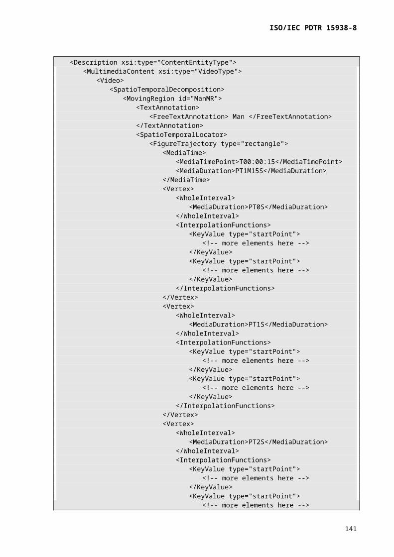
ISO/IEC PDTR 15938-8
<InkSegment><InkMediaInformation>
<WritingFieldLayout fieldIDList="HealthCondition"><Polygon>
<Coords mpeg7:dim="8"> 15 225 -6 45 0 0 6 </Coords>
</Polygon></WritingFieldLayout><OverlaidMedia fieldIDRef="HealthCondition"
scaleX="0.3333"><OverlaidMediaLocator>
<MediaUri>http://www.mpeg7.org/demo.txt</MediaUri></OverlaidMediaLocator><MediaRegionLocator>
<Polygon><Coords mpeg7:dim="8"> 5 75 0 -2 15 0 0 2
</Coords></Polygon>
</MediaRegionLocator></OverlaidMedia>
</InkMediaInformation><SceneGraphMask>
<SubGraphNum>2</SubGraphNum></SceneGraphMask>
</InkSegment></SpatialDecomposition>
</InkContent></MultimediaContent>
</Description></Mpeg7>
4.8.8.3 HandWritingRecogInformation DS
4.8.8.3.1 HandWritingRecogInformation DS examples
The following example illustrates the use of the HandWritingRecogInformation DS for describing information about a hand-writing recognizer named "Super Recog 1", which uses a lexicon with 20 entries representing names of people.
<Mpeg7><Description xsi:type="ContentEntityType">
<MultimediaContent xsi:type="InkContentType"><InkContent>
<HandWritingRecogInformation><Recognizer>
<Name><Name> Super Recog 1 </Name>
</Name></Recognizer><InkLexicon>
<Entry index="item0"><Text>
<Name> Ann </Name></Text><InkSegmentRef href="#Electro0"/>
</Entry><Entry index="item1">
<Text>
143

ISO/IEC PDTR 15938-8
<Name> Juan </Name></Text><InkSegmentRef href="#Electro1"/>
</Entry><!-- more elements here --><Entry index="item20">
<Text><Name> Beatriz </Name>
</Text><InkSegmentRef href="#Electro20"/>
</Entry></InkLexicon>
</HandWritingRecogInformation></InkContent>
</MultimediaContent></Description>
</Mpeg7>
4.8.8.4 HandWritingRecogResult DS
4.8.8.4.1 HandWritingRecogResult DS examples
The following example illustrates the use of the HandWritingRecogResult DS for describing the hand-writing recognition results for the word "Ana". The recognizer returns two results one of which corresponds to a lexicon entry in the HandWritingRecogInformation DS example in 4.8.8.3.1.
<Mpeg7><Description xsi:type="ContentEntityType">
<MultimediaContent xsi:type="InkContentType"><InkContent>
<HandWritingRecogResult><Quality>0.6</Quality><Result score="0.7">
<Text> Ana </Text></Result><Result score="0.54">
<LexiconIndexRef idref="#item0"/></Result>
</HandWritingRecogResult></InkContent>
</MultimediaContent></Description>
</Mpeg7>
4.8.8.5 Ink segment decomposition tools
Information on extraction and use is not provided.
4.8.9 Video editing segment description tools
4.8.9.1 AnalyticEditedVideoSegment DS
Information on extraction and use is not provided.
144

ISO/IEC PDTR 15938-8
4.8.9.2 Analytic edited video segment decomposition tools
4.8.9.3 EditedVideo DS
4.8.9.4 Edited video decomposition tools
4.8.9.5 AnalyticClip DS
4.8.9.6 Shot DS
Information on extraction and use is not provided.
4.8.9.7 Shot decomposition tools
Information on extraction and use is not provided.
4.8.9.8 CompositionShot DS
Information on extraction and use is not provided.
4.8.9.9 Composition shot decomposition tools
Information on extraction and use is not provided.
4.8.9.10 IntraCompositionShot DS
Information on extraction and use is not provided.
4.8.9.11 Intra-composition shot decomposition tools
Information on extraction and use is not provided.
4.8.9.12 AnalyticTransition DS
Information on extraction and use is not provided.
4.8.9.13 CompositionTransition DS
Information on extraction and use is not provided.
4.8.9.14 InternalTransition DS
Information on extraction and use is not provided.
4.8.9.15 EditedMovingRegion DS
Information on extraction and use is not provided.
4.8.9.16 Video editing segment description tools examples
4.8.9.16.1 Description of a sequence of composition shots and internal transitions
The following example illustrates the use of the AnalyticClip DS and the AnalyticTransition DS for describing a video content that contains a single shot with two composition shots and an internal transition.
145

ISO/IEC PDTR 15938-8
<Mpeg7><Description xsi:type="ContentEntityType">
<MultimediaContent xsi:type="AnalyticEditedVideoType"><AnalyticEditedVideo xsi:type="EditedVideoType">
<MediaLocator><MediaUri>video.mpg</MediaUri>
</MediaLocator><!-- more elements here --><AnalyticEditingTemporalDecomposition gap="false"
overlap="false"><!-- Description of Eyexam --><Shot id="ClipS_3" locationReliability="0.9"
editingLevelReliability="0.5"><MediaTime>
<MediaRelIncrTimePoint mediaTimeUnit="PT1N25F"
mediaTimeBase="../../../../MediaLocator[1]">35</MediaRelIncrTimePoint><MediaIncrDuration
mediaTimeUnit="PT1N25F">413</MediaIncrDuration></MediaTime><AnalyticEditingTemporalDecomposition gap="false"
overlap="false"><CompositionShot id="ClipCS_1"
locationReliability="0.9" editingLevelReliability="0.5" type="simple"><MediaTime>
<MediaRelIncrTimePoint mediaTimeUnit="PT1N25F"
mediaTimeBase="../../../../../../MediaLocator[1]">35</MediaRelIncrTimePoint>
<MediaIncrDuration
mediaTimeUnit="PT1N25F">55</MediaIncrDuration></MediaTime>
</CompositionShot><CompositionTransition id="CT_1"
locationReliability="0.9" editingLevelReliability="0.5"
evolutionReliability="0.5"><MediaTime>
<MediaRelIncrTimePoint mediaTimeUnit="PT1N25F"
mediaTimeBase="../../../../../../MediaLocator[1]">90</MediaRelIncrTimePoint>
<MediaIncrDuration
mediaTimeUnit="PT1N25F">10</MediaIncrDuration></MediaTime><EvolutionType href="...">
<Name>IrisOpen</Name></EvolutionType>
</CompositionTransition><CompositionShot id="ClipCS_2"
locationReliability="0.9" editingLevelReliability="0.5"><MediaTime>
146

ISO/IEC PDTR 15938-8
<MediaRelIncrTimePoint mediaTimeUnit="PT1N25F"
mediaTimeBase="../../../../../../MediaLocator[1]">100</MediaRelIncrTimePoint>
<MediaIncrDuration
mediaTimeUnit="PT1N25F">348</MediaIncrDuration></MediaTime><AnalyticEditingTemporalDecomposition
gap="false" overlap="false"><IntraCompositionShot id="ClipICS_1"
locationReliability="0.9" editingLevelReliability="0.5"
type="simple"><MediaTime>
<MediaRelIncrTimePoint mediaTimeUnit="PT1N25F" mediaTimeBase="../../../../../../../../MediaLocator[1]">100</MediaRelIncrTimePoint>
<MediaIncrDuration
mediaTimeUnit="PT1N25F">75</MediaIncrDuration></MediaTime>
</IntraCompositionShot><InternalTransition id="IT_1"
locationReliability="0.9" editingLevelReliability="0.5" evolutionReliability="0.5"><MediaTime>
<MediaRelIncrTimePoint mediaTimeUnit="PT1N25F" mediaTimeBase="../../../../../../../../MediaLocator[1]">175</MediaRelIncrTimePoint>
<MediaIncrDuration
mediaTimeUnit="PT1N25F">8</MediaIncrDuration></MediaTime><EvolutionType href="...">
<Name xml:lang="en">crossdissolve</Name>
</EvolutionType></InternalTransition><IntraCompositionShot id="ClipICS_2"
locationReliability="0.9" editingLevelReliability="0.5"
type="simple"><MediaTime>
<MediaRelIncrTimePoint mediaTimeUnit="PT1N25F" mediaTimeBase="../../../../../../../../MediaLocator[1]">183</MediaRelIncrTimePoint>
<MediaIncrDuration
mediaTimeUnit="PT1N25F">265</MediaIncrDuration></MediaTime>
</IntraCompositionShot></AnalyticEditingTemporalDecomposition>
</CompositionShot>
147

ISO/IEC PDTR 15938-8
</AnalyticEditingTemporalDecomposition></Shot>
</AnalyticEditingTemporalDecomposition></AnalyticEditedVideo>
</MultimediaContent></Description>
</Mpeg7>
4.8.9.16.2 Description of a shot associated to a composite clip
The following examples illustrate the use of the AnalyticClip DS, the AnalyticTransition DS, and the EditedMovingRegion DS for describing a shot that is a composite clip. In the first example, there are no internal transitions: the analytic clip is a composite clip and a shot.
<Mpeg7><Description xsi:type="ContentEntityType">
<MultimediaContent xsi:type="AnalyticEditedVideoType"><AnalyticEditedVideo xsi:type="EditedVideoType">
<MediaLocator><MediaUri>video.mpg</MediaUri>
</MediaLocator><AnalyticEditingTemporalDecomposition gap="false"
overlap="false"><Shot id="ClipS_3" locationReliability="0.9"
editingLevelReliability="0.5" type="composite"><MediaTime>
<MediaRelIncrTimePoint mediaTimeUnit="PT1N25F"
mediaTimeBase="../../../../MediaLocator[1]">35</MediaRelIncrTimePoint><MediaIncrDuration
mediaTimeUnit="PT1N25F">413</MediaIncrDuration></MediaTime>
</Shot></AnalyticEditingTemporalDecomposition>
</AnalyticEditedVideo></MultimediaContent>
</Description></Mpeg7>
In the second example, the shot is temporally decomposed into several composition shots; and the composition shots are temporally decomposed into intra-composition shots. The edition areas in the shot, composition shots and intra-composition shots are described using the EditedMovingRegion DS as the result of the spatio-temporal decomposition of the analytic edited video segments, i.e., using the AnalyticEditedVideoSegmentSpatioTemporalDecomposition DS. In composition and internal transition descriptions, the edited moving regions introduced or affected by the transitions are referenced by using the EditedMovingRegionRef element in the AnalyticTransition DS.
<Mpeg7><Description xsi:type="ContentEntityType">
<MultimediaContent xsi:type="AnalyticEditedVideoType"><AnalyticEditedVideo xsi:type="EditedVideoType">
<MediaLocator><MediaUri>video.mpg</MediaUri>
</MediaLocator><AnalyticEditingTemporalDecomposition gap="false"
overlap="false"><!-- Description of Eyexam --><Shot id="ClipS_3" locationReliability="0.9"
148

ISO/IEC PDTR 15938-8
editingLevelReliability="0.5" type="composite"><MediaTime>
<MediaRelIncrTimePoint mediaTimeUnit="PT1N25F"
mediaTimeBase="../../../../MediaLocator[1]">35</MediaRelIncrTimePoint><MediaIncrDuration
mediaTimeUnit="PT1N25F">413</MediaIncrDuration></MediaTime><AnalyticEditionAreaDecomposition gap="false"
overlap="true" criteria="edition area"><EditedMovingRegion id="editArea_1">
<TextAnnotation><FreeTextAnnotation> Frame area
</FreeTextAnnotation></TextAnnotation><SpatioTemporalLocator>
<FigureTrajectory type="rectangle"><MediaTime>
<MediaRelIncrTimePoint mediaTimeUnit="PT1N25F" mediaTimeBase="../../../../../../../../MediaLocator[1]">35</MediaRelIncrTimePoint>
<MediaIncrDuration
mediaTimeUnit="PT1N25F">413</MediaIncrDuration></MediaTime><Vertex>
<WholeInterval><MediaDuration>PT0S</MediaDuration>
</WholeInterval><InterpolationFunctions>
<KeyValue type="startPoint"><!-- more elements here -->
</KeyValue><KeyValue type="startPoint">
<!-- more elements here --></KeyValue>
</InterpolationFunctions></Vertex><Vertex>
<WholeInterval><MediaDuration>PT1S</MediaDuration>
</WholeInterval><InterpolationFunctions>
<KeyValue type="startPoint"><!-- more elements here -->
</KeyValue><KeyValue type="startPoint">
<!-- more elements here --></KeyValue>
</InterpolationFunctions></Vertex><Vertex>
<WholeInterval><MediaDuration>PT2S</MediaDuration>
</WholeInterval><InterpolationFunctions>
<KeyValue type="startPoint"><!-- more elements here -->
</KeyValue>
149

ISO/IEC PDTR 15938-8
<KeyValue type="startPoint"><!-- more elements here -->
</KeyValue></InterpolationFunctions>
</Vertex><!-- more elements here -->
</FigureTrajectory></SpatioTemporalLocator><RegionDepthType href="...">
<Name xml:lang="en">background</Name></RegionDepthType>
</EditedMovingRegion><EditedMovingRegion id="editArea_2">
<TextAnnotation>
<FreeTextAnnotation>CenteredCercle</FreeTextAnnotation></TextAnnotation><SpatioTemporalLocator>
<FigureTrajectory type="rectangle"><MediaTime>
<MediaRelIncrTimePoint mediaTimeUnit="PT1N25F" mediaTimeBase="../../../../../../../../MediaLocator[1]">175</MediaRelIncrTimePoint>
<MediaIncrDuration
mediaTimeUnit="PT1N25F">273</MediaIncrDuration></MediaTime><Vertex>
<WholeInterval><MediaDuration>PT0S</MediaDuration>
</WholeInterval><InterpolationFunctions>
<KeyValue type="startPoint"><!-- more elements here -->
</KeyValue><KeyValue type="startPoint">
<!-- more elements here --></KeyValue>
</InterpolationFunctions></Vertex><Vertex>
<WholeInterval><MediaDuration>PT1S</MediaDuration>
</WholeInterval><InterpolationFunctions>
<KeyValue type="startPoint"><!-- more elements here -->
</KeyValue><KeyValue type="startPoint">
<!-- more elements here --></KeyValue>
</InterpolationFunctions></Vertex><Vertex>
<WholeInterval><MediaDuration>PT2S</MediaDuration>
</WholeInterval><InterpolationFunctions>
<KeyValue type="startPoint"><!-- more elements here -->
150
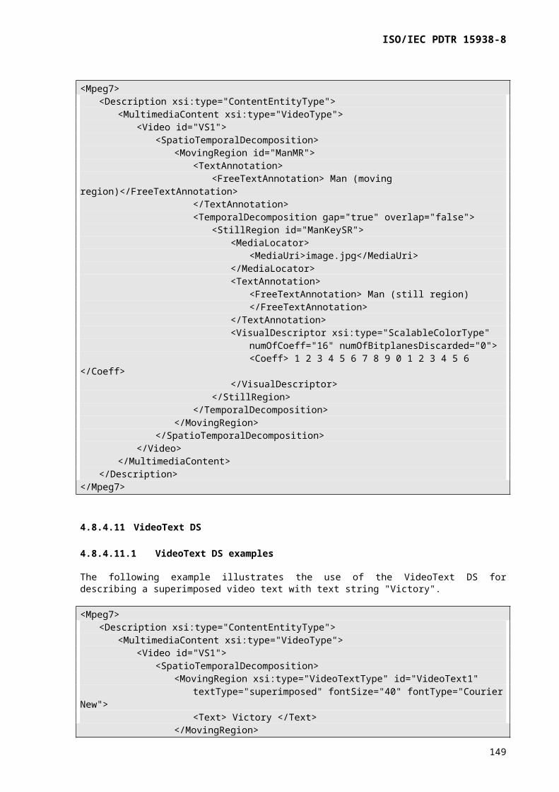
ISO/IEC PDTR 15938-8
</KeyValue><KeyValue type="startPoint">
<!-- more elements here --></KeyValue>
</InterpolationFunctions></Vertex><!-- more elements here -->
</FigureTrajectory></SpatioTemporalLocator><RegionDepthType href="...">
<Name xml:lang="en">foreground</Name></RegionDepthType>
</EditedMovingRegion></AnalyticEditionAreaDecomposition><AnalyticEditingTemporalDecomposition gap="false"
overlap="false"><CompositionShot id="ClipCS_1"
locationReliability="0.9" editingLevelReliability="0.5" type="simple"><MediaTime>
<MediaRelIncrTimePoint mediaTimeUnit="PT1N25F"
mediaTimeBase="../../../../../../MediaLocator[1]">35</MediaRelIncrTimePoint>
<MediaIncrDuration
mediaTimeUnit="PT1N25F">55</MediaIncrDuration></MediaTime>
</CompositionShot><CompositionTransition id="CT_1"
locationReliability="0.9" editingLevelReliability="0.5"
evolutionReliability="0.5"><MediaTime>
<MediaRelIncrTimePoint mediaTimeUnit="PT1N25F"
mediaTimeBase="../../../../../../MediaLocator[1]">90</MediaRelIncrTimePoint>
<MediaIncrDuration
mediaTimeUnit="PT1N25F">10</MediaIncrDuration></MediaTime><EvolutionType href="...">
<Name xml:lang="en">IrisOpen</Name></EvolutionType><!--Edition area introduced by composition
transition --><EditedMovingRegionRef href="#editArea_2"/>
</CompositionTransition><CompositionShot id="ClipCS_2"
locationReliability="0.9" editingLevelReliability="0.5" type="composite"><MediaTime>
<MediaRelIncrTimePoint mediaTimeUnit="PT1N25F"
151

ISO/IEC PDTR 15938-8
mediaTimeBase="../../../../../../MediaLocator[1]">100</MediaRelIncrTimePoint>
<MediaIncrDuration
mediaTimeUnit="PT1N25F">348</MediaIncrDuration></MediaTime><AnalyticEditingTemporalDecomposition
gap="false" overlap="true"><IntraCompositionShot id="ClipICS_1"
locationReliability="0.9" editingLevelReliability="0.5"
type="simple"><MediaTime>
<MediaRelIncrTimePoint mediaTimeUnit="PT1N25F" mediaTimeBase="../../../../../../../../MediaLocator[1]">100</MediaRelIncrTimePoint>
<MediaIncrDuration
mediaTimeUnit="PT1N25F">75</MediaIncrDuration></MediaTime>
</IntraCompositionShot><InternalTransition id="IT_1"
locationReliability="0.9" editingLevelReliability="0.5" evolutionReliability="0.5"><MediaTime>
<MediaRelIncrTimePoint mediaTimeUnit="PT1N25F" mediaTimeBase="../../../../../../../../MediaLocator[1]">175</MediaRelIncrTimePoint>
<MediaIncrDuration
mediaTimeUnit="PT1N25F">1</MediaIncrDuration></MediaTime><EvolutionType href="...">
<Name xml:lang="en">cut</Name></EvolutionType><!--Edition area affected by inter.
transition --><EditedMovingRegionRef
href="#editArea_2"/></InternalTransition><IntraCompositionShot id="ClipICS_2"
locationReliability="0.9" editingLevelReliability="0.5"
type="simple"><MediaTime>
<MediaRelIncrTimePoint mediaTimeUnit="PT1N25F" mediaTimeBase="../../../../../../../../MediaLocator[1]">175</MediaRelIncrTimePoint>
<MediaIncrDuration
mediaTimeUnit="PT1N25F">273</MediaIncrDuration></MediaTime>
</IntraCompositionShot></AnalyticEditingTemporalDecomposition>
</CompositionShot></AnalyticEditingTemporalDecomposition>
152

ISO/IEC PDTR 15938-8
</Shot></AnalyticEditingTemporalDecomposition>
</AnalyticEditedVideo></MultimediaContent>
</Description></Mpeg7>
4.8.10 Structural relation classification schemes
4.8.10.1.1 TemporalRelation CS examples
The following example illustrates the use of the TemporalRelation CS and the Graph DS for describing the relation that video segment A is before video segment B.
<VideoSegment id="segmentA"> <!-- more elements here --> </VideoSegment><VideoSegment id="segmentB"> <!-- more elements here --> </VideoSegment><Graph>
<Node id="nodeA" href="#segmentA"/><Node id="nodeB" href="#segmentB"/><!-- Edge a->b --><Relation type="urn:mpeg:mpeg7:cs:TemporalRelationCS:2001:before"
source="#nodeB" target="#nodeA"/></Graph>
The following example illustrates the use of the TemporalRelation CS and the Relation DS for describing the relation that video segment C is before video segment D.
<VideoSegment id="segmentD"><Relation type="urn:mpeg:mpeg7:cs:TemporalRelationCS:2001:before"
target="#segmentD"/><MediaTime> <!-- more elements here --> </MediaTime>
</VideoSegment>
<VideoSegment id="segmentC"><MediaTime> <!-- more elements here --> </MediaTime>
</VideoSegment>
The following example illustrates the use of the TemporalRelation CS and the Graph DS for describing temporal relations between the narrator moving region ("narrator-movreg"), the rabbit moving region ("rabbit-movreg"), and the sun moving region ("sun-movreg") of a documentary video on the subject of nature. It is assumed that the segments have been described using the Segment DSs with the specified id attributes. There are two variations shown below: the first uses Relation and Node in the Graph DS, while the second uses only Relation.
<MovingRegion id="sun-movreg"><SpatioTemporalLocator> <!-- more elements here -->
</SpatioTemporalLocator></MovingRegion><MovingRegion id="narrator-movreg">
<SpatioTemporalLocator> <!-- more elements here --> </SpatioTemporalLocator></MovingRegion><MovingRegion id="rabbit-movreg">
<SpatioTemporalLocator> <!-- more elements here --> </SpatioTemporalLocator></MovingRegion>
153

ISO/IEC PDTR 15938-8
<!-- First variation of the temporal graph --><Graph type="temporal">
<Node id="node1" href="#sun-movreg"/><Node id="node2" href="#rabbit-movreg"/><Node id="node3" href="#narrator-movreg"/><Node id="node4" href="#sun-movreg"/><Relation type="urn:mpeg:mpeg7:cs:TemporalRelationCS:2001:starts"
source="#node2" target="#node1"/><Relation type="urn:mpeg:mpeg7:cs:TemporalRelationCS:2001:before"
source="#node4" target="#node3"/></Graph>
<!-- Second variation of the temporal graph --><Graph type="temporal">
<Relation type="urn:mpeg:mpeg7:cs:TemporalRelationCS:2001:starts"source="#rabbit-movreg" target="#sun-movreg"/>
<Relation type="urn:mpeg:mpeg7:cs:TemporalRelationCS:2001:before"source="#sun-movreg" target="#narrator-movreg"/>
</Graph>
4.8.10.2 SpatialRelation CS
4.8.10.2.1 SpatialRelation CS examples
The following example illustrates the use of the SpatialRelation CS for describing spatial relations among segments. The 2D-String is a data structure for spatial reasoning. In the following example, the 2D-string describes the spatial relations between the regions. In Figure 35, the regions correspond to the rabbit ("rabbit-rg"), cloud ("cloud-rg"), airplane ("airplane-rg"), and car ("car-rg"). The 2D-String is given as follows: (rabbit < cloud < car = airplane, rabbit = car < airplane < cloud), where the symbol "=" denotes the spatial relations "at the same x as" and "at the same y as", the symbol "<" denotes the spatial relations "left/right" and "below/above", and the symbol ":" denotes the spatial relation "in the same set as". The description of the associated 2D-String for the example in Figure 35 is included below. All the relations in this example are standard relations except for "sameX" and "sameY".
Figure 35: Example description of spatial relations in an image using 2D string.
<!-- 2D String rabbit<cloud<car=airplane, rabbit=car<airplane<cloud --><Graph>
<Relation type="urn:mpeg:mpeg7:cs:SpatialRelationCS:2001:left"source="#cloud-rg" target="#rabbit-rg"/>
<Relation type="urn:mpeg:mpeg7:cs:SpatialRelationCS:2001:left"source="#car-rg" target="#cloud-rg"/>
<Relation name=" urn:example:arelationcs:sameX"
154

ISO/IEC PDTR 15938-8
source="#airplane-rg" target="#car-rg"/><Relation name=" urn:example:arelationcs:sameY"
source="#car-rg" target="#rabbit-rg"/><Relation type="urn:mpeg:mpeg7:cs:SpatialRelationCS:2001:below"
source="#airplane-rg" target="#car-rg"/><Relation type="urn:mpeg:mpeg7:cs:SpatialRelationCS:2001:below"
source="#cloud-rg" target="#airplane-rg"/></Graph>
4.8.10.2.2 SpatialRelation CS extraction
The extraction of relations among segment can be done automatically or by hand based on different criteria (e.g. semantic and temporal information). This subclause describes the spatio-temporal structure (relation) features extracted for segmented video objects’ regions in the AMOS system and latter used for retrieval. In this subclause, spatio-temporal structure of an object is understood as the spatio-temporal relations among its composing regions.
In AMOS, given a set of regions of a semantic video object, the structure descriptors are derived from their spatial and temporal positions and boundaries. These features are pre-computed and properly stored to allow quick access and examination in the similarity matching process. AMOS uses two spatial and one temporal structure features (Figure36).
a) Spatial Orientation Graph
At1 t2
Relation vector: [t1,t2,t3]
b) Spatial Topological Graph
Relation vector: [-1,0,1]
A is contained by B
B contains C
BCt3
A-1 0
BC1
A, C not contain other
A-1 0
BC1
c) Directional TemporalGraph
Relation vector: [-1,0,1]
A starts after B
B starts before CA,C start at same time
t1 is angle of AB
t3 is angle of BCt2 is angle of AC
Ordered Region List : (A, B, C)
Figure 36: Examples of spatio-temporal relation graphs. There are several different ways to compare spatial structure, such as 2D-Strings and spatio-temporal logics . AMOS uses a relatively fast and simple method, the spatial-orientation graph, to represent spatial relations as edges in a weighted graph . This graph can be easily constructed by computing the orientation of each edge between the centroids of a pair of query regions, and stored as a n*(n-1)/2-dimension descriptor, where n is the number of query regions (Figure 36.a). The spatial-orientation graph cannot handle the "contain" relation. AMOS complements it with a topological graph (Figure 36.b), which defines the contain relation between each pair of regions with three possible values: contains (1), is-contained (-1) or not containing each other (0).
In a similarly way, the temporal graph (Figure 36.c) defines whether one region starts before (1), after (-1) or at the same time (0) with another region. Note that, for simplicity, the temporal order according to the first appearing time (or starting time) of each region is only defined. By taking the ending time, a more complicated temporal relation graph can also be generated.
155

ISO/IEC PDTR 15938-8
4.8.10.3 Structural relation classification schemes examples
The following example illustrates the use of the TemporalRelation CS and the SpatialRelation CS for describing structural relations among segments of a video segment capturing a goal in a soccer game. The video segment corresponds to id = "Goal-sg". The kick and not-catch events in the video shot are represented by video segments id = "Kick-sg" and id = "Not-Catch-sg", respectively. The spatio-temporal regions corresponding to the goal, the ball, the forward, and the goalkeeper are described by moving regions id = "Goal-rg", id = "Ball-rg", "Forward-rg", and id = "Goalkeeper-rg", respectively.
Figure 37: Examples of relationships among video segments and moving regions.
Figure 38: Examples of relationships among video segments and moving regions.
The Graph DS describes the relations between the video segments and moving regions. Examples of relations between the segments are shown in Figure 37 and Figure 38. In Figure 37 (Graph 1), the
156

ISO/IEC PDTR 15938-8
region id = "Goal-rg", the video segment id = "Kick-sg", and the video segment id = "Not-Catch-sg" are described as being temporally contained in the segment id = "Goal-sg". The video segment id = "Kick-sg" is also described as happening before the video segment id = "Not-Catch-sg".
In Figure 38 (Graph 2), the video segment id = "Kick-sg" is described as temporally containing the moving regions id = "Forward-rg" and the id = "Ball-rg". Similarly, the video segment id = "Not-Catch-sg" is described as temporally containing the moving regions id = "Ball-rg" and the id = "Goalkeeper-rg". The region id = "Goalkeeper-rg" is related to the moving region id = "Forward-rg" by a spatial relation, "Northeast". The moving region id = "Ball-rg" is related to the moving region id = "Goal-rg" by a visual, global relation, "Moves towards".
The description of the segment graphs shown in Figure 37 and Figure 38 is included below.
<!-- Description of Graph 1 --><Graph>
<Relation type="urn:mpeg:mpeg7:cs:TemporalRelationCS:2001:contains"source="#Goal-rg" target="#Goal-sg"/>
<Relation type="urn:mpeg:mpeg7:cs:TemporalRelationCS:2001:contains"source="#Kick-sg" target="#Goal-sg"/>
<Relation type="urn:mpeg:mpeg7:cs:TemporalRelationCS:2001:contains"source="#Not-Catch-sg" target="#Goal-sg"/>
<Relation type="urn:mpeg:mpeg7:cs:TemporalRelationCS:2001:before"source="#Not-Catch-sg" target="#Kick-sg"/>
</Graph>
<!-- Description of Graph 2 --><Graph>
<Relation type="urn:mpeg:mpeg7:cs:TemporalRelationCS:2001:contains"source="#Forward-rg" target="#Kick-sg"/>
<Relation type="urn:mpeg:mpeg7:cs:TemporalRelationCS:2001:contains"source="#Ball-rg" target="#kick-sg"/>
<Relation type="urn:mpeg:mpeg7:cs:TemporalRelationCS:2001:contains"source="#Ball-rg" target="#Not-Catch-sg"/>
<Relation type="urn:mpeg:mpeg7:cs:TemporalRelationCS:2001:before"source="#Goalkeeper-rg" target="#Not-Catch-sg"/>
<Relation type="urn:mpeg:mpeg7:cs:SpatialRelationCS:2001:northeast"source="#Goalkeeper-rg" target="#Forward-rg"/>
<Relation name="urn:example:arelationcs:movesToward"source="#Goal-rg" target="#Ball-rg"/>
</Graph>
157

ISO/IEC PDTR 15938-8
4.9 Semantics description tools
4.9.1 Introduction.
4.9.1.1 Overview
The tools specified in this clause include the following:
Table 10: Overview of the semantics description tools.Tool Functionality
Semantic entity description tools
These tools describe semantic entities such as objects, agent objects, events, concepts, states, places, times, and narrative worlds.
Semantic attribute description tools
These tools describe attributes of semantic entities related to abstraction in semantic descriptions and semantic measurements in time and space.
Semantic relation classification schemes
These classification schemes define semantic relations.
Figure 39 illustrates the organization of the tools for describing the semantics of multimedia content.
Figure 39: Illustration of the relationships of the tools for describing the semantics of multimedia content.
4.9.1.2 Semantics description example
Figure 40 shows an informative example of how the semantic description tools describe the semantics of an image. The boxes in Figure 40 represent descriptions of different semantic entity description tools and semantic relation classification schemes.
158

ISO/IEC PDTR 15938-8
Figure 40: Illustration of the description of a narrative world captured by an image using tools for describing the semantics of multimedia content.
The semantic description of the image is the following: "Alex is shaking hands with Ana in New York on the 9th of September. The event is showing "comradeship". In this example, the AgentObject DS, the Event DS, the SemanticPlace DS, the SemanticTime DS, and the Concept DS describe people, event, place, time and concept of the image, respectively. A Label element describes each semantic entity; the Property, Time, Place and Agent elements are also used to describe the attributes of people, event, place, time and concept of the image. The SemanticRelation CS describes the relations among semantic entities and possibly other non-semantic entities.
4.9.2 Abstraction model
Information on extraction and use is not provided.
4.9.3 Semantic entity description tools
4.9.3.1 SemanticBase DS
Information on extraction and use is not provided.
4.9.3.2 SemanticBag DS
Information on extraction and use is not provided.
4.9.3.3 Semantic DS
4.9.3.3.1 Semantic DS examples
The following example illustrates the use of the Semantic DS for describing the semantic entity "apple". The Label elements can be used as keywords or index terms for accessing this semantic description.
<Mpeg7><Description xsi:type="SemanticDescriptionType">
<Semantics id="apple"><Label>
<Name> Apple </Name>
159

ISO/IEC PDTR 15938-8
</Label><Label>
<Name> Fruit </Name></Label><Label>
<Name> Pome </Name></Label><Definition>
<FreeTextAnnotation>The fleshy usually rounded and red, yellow, or green
edible pome fruit of a tree (genus Malus) of the rose family
</FreeTextAnnotation></Definition><Property>
<Name> Juicy </Name></Property><MediaOccurrence>
<MediaLocator><MediaUri> image.jpg </MediaUri>
</MediaLocator></MediaOccurrence>
</Semantics></Description>
</Mpeg7>
4.9.3.4 Object DS
4.9.3.4.1 Object DS examples
The following example illustrates the use of the Object DS for describing a table shown in an image. In this example, the table object is decomposed into one object "tabletop" and four objects "leg", i.e., a component type of decomposition. The MediaOccurrence element is used for locating the object within the media and describing the visual features of the image.
<Mpeg7><Description xsi:type="SemanticDescriptionType">
<Semantics><Label>
<Name> Description of table </Name></Label><SemanticBase xsi:type="ObjectType">
<Label><Name> Table </Name>
</Label><Definition>
<FreeTextAnnotation>Piece of furniture consisting of a smooth flat slab fixed on legs
</FreeTextAnnotation></Definition><MediaOccurrence>
<MediaLocator><MediaUri>image.jpg</MediaUri>
</MediaLocator><VisualDescriptor xsi:type="ScalableColorType"
numOfCoeff="16" numOfBitplanesDiscarded="0"><Coeff> 1 2 3 4 5 6 7 8 9 0 1 2 3 4 5 6 </Coeff>
160

ISO/IEC PDTR 15938-8
</VisualDescriptor></MediaOccurrence><Object id="tabletop-object">
<Label><Name> Table top </Name>
</Label><MediaOccurrence>
<MediaLocator><MediaUri>image.jpg</MediaUri>
</MediaLocator><Mask xsi:type="SpatialMaskType">
<SubRegion><Polygon>
<Coords mpeg7:dim="2 5"> 5 25 10 20 15 15 10 10 5 15
</Coords></Polygon>
</SubRegion></Mask><VisualDescriptor xsi:type="ScalableColorType"
numOfCoeff="16" numOfBitplanesDiscarded="0"><Coeff> 1 2 3 4 5 6 7 8 9 0 1 2 3 4 5 6 </Coeff>
</VisualDescriptor></MediaOccurrence>
</Object><Object id="Leg1-object">
<Label><Name> Leg </Name>
</Label><MediaOccurrence>
<MediaLocator><MediaUri>image.jpg</MediaUri>
</MediaLocator><Mask xsi:type="SpatialMaskType">
<SubRegion><Polygon>
<Coords mpeg7:dim="2 5"> 5 25 10 20 15 15 10 10 5 15
</Coords></Polygon>
</SubRegion></Mask><VisualDescriptor xsi:type="ScalableColorType"
numOfCoeff="16" numOfBitplanesDiscarded="0"><Coeff> 1 2 3 4 5 6 7 8 9 0 1 2 3 4 5 6 </Coeff>
</VisualDescriptor></MediaOccurrence>
</Object><Object id="Leg2-object">
<Label><Name> Leg </Name>
</Label><MediaOccurrence>
<MediaLocator><MediaUri>image.jpg</MediaUri>
</MediaLocator><Mask xsi:type="SpatialMaskType">
<SubRegion><Polygon>
161

ISO/IEC PDTR 15938-8
<Coords mpeg7:dim="2 5"> 5 25 10 20 15 15 10 10 5 15
</Coords></Polygon>
</SubRegion></Mask><VisualDescriptor xsi:type="ScalableColorType"
numOfCoeff="16" numOfBitplanesDiscarded="0"><Coeff> 1 2 3 4 5 6 7 8 9 0 1 2 3 4 5 6 </Coeff>
</VisualDescriptor></MediaOccurrence>
</Object><Object id="Leg3-object">
<Label><Name> Leg </Name>
</Label><MediaOccurrence>
<MediaLocator><MediaUri>image.jpg</MediaUri>
</MediaLocator><Mask xsi:type="SpatialMaskType">
<SubRegion><Polygon>
<Coords mpeg7:dim="2 5"> 5 25 10 20 15 15 10 10 5 15
</Coords></Polygon>
</SubRegion></Mask><VisualDescriptor xsi:type="ScalableColorType"
numOfCoeff="16" numOfBitplanesDiscarded="0"><Coeff> 1 2 3 4 5 6 7 8 9 0 1 2 3 4 5 6 </Coeff>
</VisualDescriptor></MediaOccurrence>
</Object><Object id="Leg4-object">
<Label><Name> Leg </Name>
</Label><MediaOccurrence>
<MediaLocator><MediaUri>image.jpg</MediaUri>
</MediaLocator><Mask xsi:type="SpatialMaskType">
<SubRegion><Polygon>
<Coords mpeg7:dim="2 5"> 5 25 10 20 15 15 10 10 5 15
</Coords></Polygon>
</SubRegion></Mask><VisualDescriptor xsi:type="ScalableColorType"
numOfCoeff="16" numOfBitplanesDiscarded="0"><Coeff> 1 2 3 4 5 6 7 8 9 0 1 2 3 4 5 6 </Coeff>
</VisualDescriptor></MediaOccurrence>
</Object>
162

ISO/IEC PDTR 15938-8
</SemanticBase></Semantics>
</Description></Mpeg7>
4.9.3.5 AgentObject DS
4.9.3.5.1 AgentObject DS examples
The following example illustrates the use of the AgentObject DS for describing a person named Alexander (Alex) Green.
<Mpeg7><Description xsi:type="SemanticDescriptionType">
<Semantics><Label>
<Name> Description of person </Name></Label><SemanticBase xsi:type="AgentObjectType">
<Label><Name> Student </Name>
</Label><Definition>
<FreeTextAnnotation> Student named Alexander Green</FreeTextAnnotation>
</Definition><Agent xsi:type="PersonType">
<Name><GivenName abbrev="Alex"> Alexander </GivenName><FamilyName> Green </FamilyName>
</Name></Agent>
</SemanticBase></Semantics>
</Description></Mpeg7>
The following example illustrates the use of the AgentObject DS for describing members of a baeball team. In this example, the agent object (Baseball team) is composed of three agent objects (players – pitcher, catcher, and third base).
<Mpeg7><Description xsi:type="SemanticDescriptionType">
<Semantics><Label>
<Name> Baseball team </Name></Label><SemanticBase xsi:type="AgentObjectType">
<Label><Name> NY Mets </Name>
</Label><Object xsi:type="AgentObjectType" id="player1-agent">
<Label href="urn:example:baseball"><Name> Pitcher </Name>
</Label><Agent xsi:type="PersonType">
<Name><GivenName> Al </GivenName>
163

ISO/IEC PDTR 15938-8
<FamilyName> Leiter </FamilyName></Name>
</Agent></Object><Object xsi:type="AgentObjectType" id="player1-agent">
<Label href="urn:example:baseball"><Name> Catcher </Name>
</Label><Agent xsi:type="PersonType">
<Name><GivenName> Mike </GivenName><FamilyName> Piazza </FamilyName>
</Name></Agent>
</Object><Object xsi:type="AgentObjectType" id="player1-agent"><Label href="urn:example:baseball">
<Name> Third base </Name></Label><Agent xsi:type="PersonType">
<Name><GivenName> Robin </GivenName><FamilyName> Ventura </FamilyName>
</Name></Agent>
</Object></SemanticBase>
</Semantics></Description>
</Mpeg7>
4.9.3.6 Event DS
4.9.3.6.1 Event DS examples
The following example illustrates the use of the Event DS for describing the event of a "handshake between two colleagues". In this example, the Relation DS uses the SemanticRelation CS to describe the agentOf and accompanierOf of the action, respectively.
<Mpeg7><Description xsi:type="SemanticDescriptionType">
<Semantics><Label>
<Name> Shake hands </Name></Label><SemanticBase xsi:type="AgentObjectType" id="AOa">
<Label href="urn:example:acs"><Name> Person A </Name>
</Label></SemanticBase><SemanticBase xsi:type="AgentObjectType" id="AOb">
<Label href="urn:example:acs"><Name> Person B </Name>
</Label></SemanticBase><SemanticBase xsi:type="EventType" id="EV1">
<Label href="urn:example:acs"><Name> Shake hands </Name>
</Label>
164

ISO/IEC PDTR 15938-8
<Definition><FreeTextAnnotation>
Clasping of right hands by two people.</FreeTextAnnotation>
</Definition><Relation
type="urn:mpeg:mpeg7:cs:SemanticRelationCS:2001:agentOf" source="#AOa" target="#AOb"/>
<Relation
type="urn:mpeg:mpeg7:cs:SemanticRelationCS:2001:accompanierOf" source="#AOb" target="#AOa"/>
</SemanticBase></Semantics>
</Description></Mpeg7>
4.9.3.7 Concept DS
4.9.3.7.1 Concept DS examples
The following example illustrates the use of the Concept DS for describing the concept "freedom" as as having properties of "open", "outspoken", and "frank". In this example, the description identifies an image of the Statue of Liberty that symbolizes "freedom".
<Mpeg7><Description xsi:type="SemanticDescriptionType">
<Semantics><Label>
<Name> Concept of freedom </Name></Label><SemanticBase xsi:type="ConceptType" id="freedom">
<Label><Name> Freedom </Name>
</Label><Property>
<Name> Open </Name></Property><Property>
<Name> Outspoken </Name></Property><Property>
<Name> Frank </Name></Property><MediaOccurrence type="symbol">
<MediaLocator><MediaUri> liberty.gif</MediaUri>
</MediaLocator></MediaOccurrence>
</SemanticBase></Semantics>
</Description></Mpeg7>
165

ISO/IEC PDTR 15938-8
4.9.3.8 SemanticState DS
4.9.3.8.1 SemanticState DS examples
The following example illustrates the use of the SemanticState DS for describing semantic attributes of a sunset. In this example, the event "sunset-event" represents the event "sunset" and the semantic state "sunset-state" describes the semantic attributes of the event "sunset". A graph relates the event "sunset-event" and the semantic state "sunset-state". A sunset is considered as an event because it can be nominalized: "The sunset is beautiful".
<Mpeg7><Description xsi:type="SemanticDescriptionType">
<Semantics><Label>
<Name> Sunset </Name></Label><SemanticBase xsi:type="EventType" id="sunset-event">
<Label><Name> Sunset </Name>
</Label></SemanticBase><SemanticBase xsi:type="SemanticStateType" id="sunset-state">
<Label><Name> State of sunset </Name>
</Label><AttributeValuePair>
<Attribute><Name> Blue </Name>
</Attribute><IntegerValue>90</IntegerValue>
</AttributeValuePair><AttributeValuePair>
<Attribute><Name> Pink </Name>
</Attribute><IntegerValue>9</IntegerValue>
</AttributeValuePair><AttributeValuePair>
<Attribute><Name> Orange </Name>
</Attribute><IntegerValue>50</IntegerValue>
</AttributeValuePair><AttributeValuePair>
<Attribute><Name> Yellow </Name>
</Attribute><IntegerValue>45</IntegerValue>
</AttributeValuePair></SemanticBase><Graph>
<!-- Relate event sunset-event and state sunset-state --><Relation
type="urn:mpeg:mpeg7:cs:SemanticRelationCS:2001:hasStateOf" source="#sunset-state" target="#sunset-event"/>
</Graph></Semantics>
</Description></Mpeg7>
166

ISO/IEC PDTR 15938-8
The following example illustrates the use of the SemanticState DS for describing the place and event for a person. In this example, "John is in Singapore today" is described by linking the AgentObject DS description corresponding to "John", the SemanticPlace DS description of "Singapore", and the SemanticTime DS description of "today" using the state "position-state". This description may be represented by an event "Being" taking place during semantic time "today" in semantic place "Singapore".
<Mpeg7><Description xsi:type="SemanticDescriptionType">
<Semantics><Label>
<Name> Place and time for a person </Name></Label><SemanticBase xsi:type="AgentObjectType" id="agent-person">
<Label><Name> John </Name>
</Label><Relation
type="urn:mpeg:mpeg7:cs:SemanticRelationCS:2001:stateOf" target="#position-state"/>
</SemanticBase><SemanticBase xsi:type="SemanticStateType" id="position-state">
<Label><Name> Position </Name>
</Label><AttributeValuePair>
<Attribute><Name> Position </Name>
</Attribute><IntegerValue>1</IntegerValue>
</AttributeValuePair><SemanticTime>
<Label><Name> today </Name>
</Label></SemanticTime><SemanticPlace>
<Label><Name> Singapore </Name>
</Label></SemanticPlace>
</SemanticBase></Semantics>
</Description></Mpeg7>
4.9.3.9 SemanticPlace DS
4.9.3.9.1 SemanticPlace DS examples
The following example illustrates the use of the SemanticPlace DS for describing the location "Columbia University in the City of New York".
<Mpeg7><Description xsi:type="SemanticDescriptionType">
<Semantics><Label>
<Name> Semantic place for Columbia University </Name></Label>
167
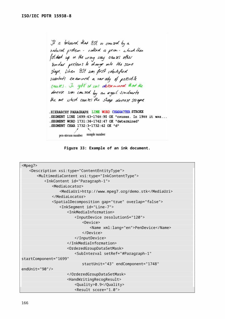
ISO/IEC PDTR 15938-8
<SemanticBase xsi:type="SemanticPlaceType" id="columbia-location">
<Label><Name> Columbia University </Name>
</Label><Place>
<Name xml:lang="en"> Columbia University in the City of New York </Name>
<Region> us </Region><PostalAddress>
<AddressLine> 600 West 116th Street, New York, NY</AddressLine>
<PostingIdentifier> U-10027 </PostingIdentifier></PostalAddress>
</Place></SemanticBase>
</Semantics></Description>
</Mpeg7>
The following example illustrates the use of the SemanticPlaceInterval element in SemanticPlace DS for describing the location "4 miles".
<Mpeg7><Description xsi:type="SemanticDescriptionType">
<Semantics><Label>
<Name> Semantic place for location four miles </Name></Label><SemanticBase xsi:type="SemanticPlaceType" id="miles4-place">
<Label><Name> 4 miles </Name>
</Label><SemanticPlaceInterval>
<Extent measurementType="length" unit="mile" value="4"/></SemanticPlaceInterval>
</SemanticBase></Semantics>
</Description></Mpeg7>
The following example illustrates the use of the SemanticPlaceInterval element in SemanticPlace DS for describing the location "Within 4 miles radius of New York City".
<Mpeg7><Description xsi:type="SemanticDescriptionType">
<Semantics><Label>
<Name> Semantic place for four mile radius of NYC </Name></Label><SemanticBase xsi:type="SemanticPlaceType" id="miles4NYC-place">
<Label><Name> Within 4 miles radius of New York City </Name>
</Label><SemanticPlaceInterval>
<Position origin="New York City"/><Extent measurementType="area" unit="square miles"
value="16*pi"/>
168

ISO/IEC PDTR 15938-8
</SemanticPlaceInterval></SemanticBase>
</Semantics></Description>
</Mpeg7>
The following example illustrates the use of the SemanticPlaceInterval element in SemanticPlace DS for describing the location "5 kilometers north of New York City and 40 kilometers east of Boston".
<Mpeg7><Description xsi:type="SemanticDescriptionType">
<Semantics><Label>
<Name> Semantic place for location near NYC and Boston </Name></Label><SemanticBase xsi:type="SemanticPlaceType" id="NYCBoston-place">
<Label><Name>
5 kilometers north of New York City and 40 kilometers east of Boston
</Name></Label><SemanticPlaceInterval>
<Position origin="New York City"><Displacement measurementType="length"
unit="kilometers" value="5"/>
<Direction measurementType="direction" unit="direction" value="north"/>
</Position></SemanticPlaceInterval><SemanticPlaceInterval>
<Position origin="Boston"><Displacement measurementType="length"
unit="kilometers" value="40"/>
<Direction measurementType="direction" unit="direction" value="east"/>
</Position></SemanticPlaceInterval>
</SemanticBase></Semantics>
</Description></Mpeg7>
If a semantic place is complex, relations may relate the location to the other semantic entities such as objects and events needed to fully describe it. The following example illustrates the use of the SemanticPlace DS for describing the location "the place where Cri and Ale got engaged."
In this example, the location "at the Eiffel Tower in the same spot where Cri and Ale were engaged last year" and the event "Spot at the Eiffel Tower" are described in the semantic entities "sem2-loc" and "engagement-event", respectively. The new semantic place ("sem2-loc") can be defined as the same as the SemanticPlace DS description of the event "engagement-event" – relation identifiedWith to semantic place "Eiffel-loc" (possibility one) - or as being the location where that event took place– relation hasLocationOf to the event "engagement-event" (possibility two). In general, if the same semantic entity is described by multiple semantic descriptions, the relationship of the descriptions can be described using the semantic relation identifiedWith.
169

ISO/IEC PDTR 15938-8
<Mpeg7><Description xsi:type="SemanticDescriptionType">
<Semantics><Label>
<Name> The place where Cri and Ale got engaged </Name></Label><SemanticBase xsi:type="SemanticPlaceType" id="sem2-loc">
<Label><Name> Eiffel Tower </Name>
</Label><Relation
type="urn:mpeg:mpeg7:cs:SemanticRelationCS:2001:identifiedWith" target="#Eiffel-loc"/>
<Relation
type="urn:mpeg:mpeg7:cs:SemanticRelationCS:2001:hasLocationOf" target="#engagement-event"/>
</SemanticBase><SemanticBase xsi:type="EventType" id="engagement-event">
<Label><Name> Engagement </Name>
</Label><Definition>
<FreeTextAnnotation>Engagement of Cri and Ale, at the Eiffel Tower in Paris
</FreeTextAnnotation></Definition><Relation
type="urn:mpeg:mpeg7:cs:SemanticRelationCS:2001:locationOf" target="#Eiffel-loc"/>
<Relation type="urn:mpeg:mpeg7:cs:SemanticRelationCS:2001:timeOf"
target="#lastyear-time"/></SemanticBase><SemanticBase xsi:type="SemanticPlaceType" id="Eiffel-loc">
<Label><Name> Spot at the Eiffel Tower </Name>
</Label></SemanticBase><SemanticBase xsi:type="SemanticTimeType" id="lastyear-time">
<Label><Name> Last year </Name>
</Label><SemanticTimeInterval>
<TimePoint origin="now"><Displacement measurementType="length" unit="year"
value="1"/><Direction measurementType="direction" unit="direction"
value="before"/></TimePoint>
</SemanticTimeInterval></SemanticBase>
</Semantics></Description>
</Mpeg7>
170

ISO/IEC PDTR 15938-8
4.9.3.10 SemanticTime DS
4.9.3.10.1 SemanticTime DS examples
The following example illustrates the use of the Time DS in SemanticTime DS for describing the time "10 days starting at 14:13:00 hours, 12 November, 2001".
<Mpeg7><Description xsi:type="SemanticDescriptionType">
<Semantics><Label>
<Name> 10 days </Name></Label><SemanticBase xsi:type="SemanticTimeType">
<Label><Name>
10 days starting at 14:13:00 hours, 12 November, 2001</Name>
</Label><Time>
<TimePoint>2001-11-12T14:13+01:00</TimePoint><Duration>P10D</Duration>
</Time></SemanticBase>
</Semantics></Description>
</Mpeg7>
The following example illustrates the use of the SemanticTimeInterval element in SemanticTime DS for describing the time "4 weeks".
<Mpeg7><Description xsi:type="SemanticDescriptionType">
<Semantics><Label>
<Name> Description of 4 weeks </Name></Label><SemanticBase xsi:type="SemanticTimeType">
<Label><Name> 4 weeks </Name>
</Label><SemanticTimeInterval>
<Duration measurementType="length" unit="week" value="4"/></SemanticTimeInterval>
</SemanticBase></Semantics>
</Description></Mpeg7>
The following example illustrates the use of the SemanticTimeInterval element in SemanticTime DS for describing the time "during 1997".
<Mpeg7><Description xsi:type="SemanticDescriptionType">
<Semantics><Label>
<Name> Description of 1997 </Name></Label>
171
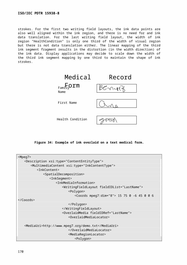
ISO/IEC PDTR 15938-8
<SemanticBase xsi:type="SemanticTimeType"><Label>
<Name> During 1997 </Name></Label><SemanticTimeInterval>
<TimePoint origin="January 1, 1997"><Displacement measurementType="length" unit="year"
value="1"/><Direction measurementType="during" unit="direction"
value="after"/></TimePoint>
</SemanticTimeInterval></SemanticBase>
</Semantics></Description>
</Mpeg7>
The following example illustrates the use of the SemanticTimeInterval element in SemanticTime DS for describing the time "last year".
<Mpeg7><Description xsi:type="SemanticDescriptionType">
<Semantics><Label>
<Name> Description of last year </Name></Label><SemanticBase xsi:type="SemanticTimeType">
<Label><Name> Last year </Name>
</Label><SemanticTimeInterval>
<TimePoint origin="now"><Displacement measurementType="length" unit="year"
value="1"/><Direction measurementType="direction" unit="direction"
value="before"/></TimePoint>
</SemanticTimeInterval></SemanticBase>
</Semantics></Description>
</Mpeg7>
The following example illustrates the use of the SemanticTimeInterval element in SemanticTime DS for describing the time "the third and fourth day in April".
<Mpeg7><Description xsi:type="SemanticDescriptionType">
<Semantics><Label>
<Name> Description of April 3 to 4 </Name></Label><SemanticBase xsi:type="SemanticTimeType">
<Label><Name> The third and fourth day in April </Name>
</Label><SemanticTimeInterval>
<TimePoint origin="April">
172

ISO/IEC PDTR 15938-8
<Displacement measurementType="length" unit="day" value="3"/>
<Direction measurementType="direction" unit="direction" value="after"/>
</TimePoint><Duration measurementType="length" unit="day" value="2"/>
</SemanticTimeInterval></SemanticBase>
</Semantics></Description>
</Mpeg7>
The following example illustrates the use of the SemanticTimeInterval element in SemanticTime DS for describing the time "Monday and Friday from 9am to 5pm".
<Mpeg7><Description xsi:type="SemanticDescriptionType">
<Semantics><Label>
<Name> Description of the time Monday and Friday 9-5 </Name></Label><SemanticBase xsi:type="SemanticTimeType">
<Label><Name> Monday and Friday from 9am to 5pm </Name>
</Label><SemanticTimeInterval>
<TimePoint origin="Monday"><Displacement measurementType="length" unit="hour"
value="9"/><Direction measurementType="direction" unit="direction"
value="after"/></TimePoint><Duration measurementType="length" unit="hour" value="8"/>
</SemanticTimeInterval><SemanticTimeInterval>
<TimePoint origin="Friday"><Displacement measurementType="length" unit="hour"
value="9"/><Direction measurementType="direction" unit="direction"
value="after"/></TimePoint><Duration measurementType="length" unit="hour" value="8"/>
</SemanticTimeInterval></SemanticBase>
</Semantics></Description>
</Mpeg7>
If a semantic time is complex, relations may relate the time to the semantic entities such as objects and events needed to fully describe it. The following example illustrates the use of the SemanticTime DS for describing the time "in the year 1899 at the same time when the earthquake happened in San Francisco".
In this example, the time "in the year 1899 at the same time when the earthquake happened in San Francisco" and the event "Earthquake in San Francisco in 1899" are described in the semantic entities "sem3-time" and "earthquake-event", respectively. The new semantic time ("sem3-time") can be defined as the same as the SemanticTime DS description of the event "earthquake-event" –
173

ISO/IEC PDTR 15938-8
relation identifiedWith to semantic time "m3_1899-time" (possibility one) - or as being the time when that event happened –relation hasTimeOf to the event "earthquake-event" (possibility two).
<Mpeg7><Description xsi:type="SemanticDescriptionType">
<Semantics><Label>
<Name> Description of time of the earthquake </Name></Label><SemanticBase xsi:type="SemanticTimeType" id="sem3-time">
<Label><Name> Time </Name>
</Label><Relation
type="urn:mpeg:mpeg7:cs:SemanticRelationCS:2001:identifiedWith" target="#m3_1899-time"/>
<Relation type="urn:mpeg:mpeg7:cs:SemanticRelationCS:2001:hasTimeOf"
target="#earthquake-event"/></SemanticBase><SemanticBase xsi:type="EventType" id="earthquake-event">
<Label><Name> Earthquake </Name>
</Label><Relation
type="urn:mpeg:mpeg7:cs:SemanticRelationCS:2001:timeOf" target="#m3_1899-time"/>
<Relation type="urn:mpeg:mpeg7:cs:SemanticRelationCS:2001:locationOf"
target="#sanfran-loc"/></SemanticBase><SemanticBase xsi:type="SemanticTimeType" id="m3_1899-time">
<Label><Name> 12 November, 1899 </Name>
</Label><Time>
<TimePoint>1899-11-12T14:13:00</TimePoint><Duration>PT3M</Duration>
</Time></SemanticBase><SemanticBase xsi:type="SemanticPlaceType" id="sanfran-loc">
<Label><Name> San Francisco </Name>
</Label></SemanticBase>
</Semantics></Description>
</Mpeg7>
4.9.3.11 Semantic entity description tools examples
The following example illustrates the use of the Semantic DS and other SemanticBase DSs for describing the narrative world of an image as shown in Figure 40. In this example, the AgentObject DS, the Event DS, the SemanticPlace DS, the SemanticTime DS, and the Concept DS describe the people, the event, the place, the time and a concept depicted or symbolized in the image. The semantic description of the image is the following: "Alex is shaking hands with Ana in New York during 1997. The event is showing as comradeship". The example assumes the image and the
174
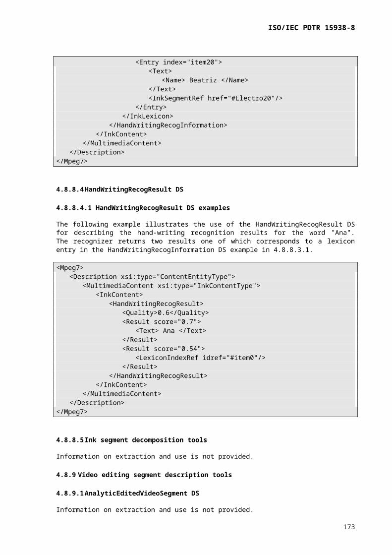
ISO/IEC PDTR 15938-8
regions of the two persons have been described using the StillRegion DS and the StillRegionSpatialDecomposition DS.
<Mpeg7 xmlns="urn:mpeg:mpeg7:schema:2001" xmlns:mpeg7="urn:mpeg:mpeg7:schema:2001" xmlns:xsi="http://www.w3.org/2001/XMLSchema-instance" xsi:schemaLocation="urn:mpeg:mpeg7:schema:2001 .\mdsfdisver3.3.xsd">
<Description xsi:type="ContentEntityType"><MultimediaContent xsi:type="ImageType">
<Image id="SR1"><SpatialDecomposition gap="true" overlap="false">
<StillRegion id="SR2"><TextAnnotation>
<FreeTextAnnotation> Alex </FreeTextAnnotation></TextAnnotation><VisualDescriptor xsi:type="ScalableColorType"
numOfCoeff="16" numOfBitplanesDiscarded="0"><Coeff> 1 2 3 4 5 6 7 8 9 0 1 2 3 4 5 6 </Coeff>
</VisualDescriptor></StillRegion><StillRegion id="SR3">
<TextAnnotation><FreeTextAnnotation> Ana </FreeTextAnnotation>
</TextAnnotation><VisualDescriptor xsi:type="ScalableColorType"
numOfCoeff="16" numOfBitplanesDiscarded="0"><Coeff> 1 2 3 4 5 6 7 8 9 0 1 2 3 4 5 6 </Coeff>
</VisualDescriptor></StillRegion>
</SpatialDecomposition></Image>
</MultimediaContent></Description><Description xsi:type="SemanticDescriptionType">
<Semantics><Label>
<Name>Semantic description of the handshake </Name></Label><SemanticBase xsi:type="EventType" id="EV1">
<Label><Name>Shake hands</Name>
</Label><Relation
type="urn:mpeg:mpeg7:cs:SemanticRelationCS:2001:agentOf" target="#AO1"/>
<Relation
type="urn:mpeg:mpeg7:cs:SemanticRelationCS:2001:accompanierOf" target="#AO2"/>
<Relation type="urn:mpeg:mpeg7:cs:SemanticRelationCS:2001:propertyOf"
target="#C1"/><Relation
type="urn:mpeg:mpeg7:cs:SemanticRelationCS:2001:mediaPerceptionOf" target="#SR1"/>
<Relation type="urn:mpeg:mpeg7:cs:SemanticRelationCS:2001:locationOf"
target="#SP1"/>
175

ISO/IEC PDTR 15938-8
<Relation type="urn:mpeg:mpeg7:cs:SemanticRelationCS:2001:timeOf"
target="#ST1"/></SemanticBase><SemanticBase xsi:type="AgentObjectType" id="AO1">
<Label><Name>Alex</Name>
</Label><Relation
type="urn:mpeg:mpeg7:cs:SemanticRelationCS:2001:mediaPerceptionOf" target="#SR2"/><Agent xsi:type="PersonType">
<Name><GivenName>Alex</GivenName>
</Name></Agent>
</SemanticBase><SemanticBase xsi:type="AgentObjectType" id="AO2">
<Label><Name>Ana</Name>
</Label><Relation
type="urn:mpeg:mpeg7:cs:SemanticRelationCS:2001:mediaPerceptionOf" target="#SR3"/>
<Agent xsi:type="PersonType"><Name>
<GivenName>Ana</GivenName></Name>
</Agent></SemanticBase><SemanticBase xsi:type="ConceptType" id="C1">
<Label><Name> Comradeship</Name>
</Label><Property>
<Name> Partnership</Name></Property><Property>
<Name> Friendship</Name></Property><Relation
type="urn:mpeg:mpeg7:cs:SemanticRelationCS:2001:symbolPerceptionOf" target="#SR1"/>
</SemanticBase><SemanticBase xsi:type="SemanticPlaceType" id="SP1">
<Label><Name>New York</Name>
</Label><Place>
<!-- more elements here --></Place>
</SemanticBase><SemanticBase xsi:type="SemanticTimeType" id="ST1">
<Label><Name> During 1997 </Name>
</Label><SemanticTimeInterval>
<TimePoint origin="January 1, 1997">
176

ISO/IEC PDTR 15938-8
<Displacement measurementType="length" unit="year" value="1"/>
<Direction measurementType="during" unit="direction" value="after"/>
</TimePoint></SemanticTimeInterval>
</SemanticBase></Semantics>
</Description></Mpeg7>
4.9.4 Semantic attribute description tools
4.9.4.1.1 AbstractionLevel datatype examples
The following example illustrates the use of the AbstractionLevel datatype in the SemanticBase DS for describing a media abstraction of the concrete semantic description shown in Figure 40. In this example, the media abstraction is the description "Alex is shaking hands with Ana in NewYork on the 9th of September" with no links to the image; this description is, therefore, applicable to any image or video depicting the event.
<!-- Media abstraction: AbstractionLevel dimension = 0 --><Mpeg7>
<Description xsi:type="SemanticDescriptionType"><Semantics>
<AbstractionLevel dimension="0"/><Label>
<Name>Alex shakes hands with Ana </Name></Label><SemanticBase xsi:type="EventType" id="EV1-MA">
<Label><Name>Shake hands</Name>
</Label><Relation
type="urn:mpeg:mpeg7:cs:SemanticRelationCS:2001:agentOf" target="#AO1-MA"/>
<Relation
type="urn:mpeg:mpeg7:cs:SemanticRelationCS:2001:acccompanierOf" target="#AO2-MA"/>
<Relation type="urn:mpeg:mpeg7:cs:SemanticRelationCS:2001:propertyOf"
target="#C1-MA"/><Relation
type="urn:mpeg:mpeg7:cs:SemanticRelationCS:2001:locationOf" target="#SP1-MA"/>
<Relation type="urn:mpeg:mpeg7:cs:SemanticRelationCS:2001:timeOf"
target="#ST1-MA"/></SemanticBase><SemanticBase xsi:type="AgentObjectType" id="AO1-MA">
<Label><Name>Alex</Name>
</Label><Agent xsi:type="PersonType">
<Name><GivenName>Alex</GivenName>
</Name></Agent>
177

ISO/IEC PDTR 15938-8
</SemanticBase><SemanticBase xsi:type="AgentObjectType" id="AO2-MA">
<Label><Name>Ana</Name>
</Label><Agent xsi:type="PersonType">
<Name><GivenName>Ana</GivenName>
</Name></Agent>
</SemanticBase><SemanticBase xsi:type="ConceptType" id="C1-MA">
<Label><Name> Comradeship</Name>
</Label><Property>
<Name> Friendship</Name></Property>
</SemanticBase><SemanticBase xsi:type="SemanticPlaceType" id="SP1-MA">
<Label><Name>Columbia University</Name>
</Label></SemanticBase><SemanticBase xsi:type="SemanticTimeType" id="ST1-MA">
<Label><Name>September 9</Name>
</Label></SemanticBase>
</Semantics></Description>
</Mpeg7>
The following example illustrates the use of the AbstractionLevel datatype in the SemanticBase DS for describing a formal abstraction of the concrete semantic description. In this example, the formal abstraction is the description "Alex is shaking hands with any woman in NewYork on the 9 th of September", where "any woman" is the variable of the formal abstraction.
<Mpeg7><Description xsi:type="SemanticDescriptionType">
<Semantics><AbstractionLevel dimension="1"/><Label>
<Name>Alex shakes hands with any woman </Name></Label><SemanticBase xsi:type="EventType" id="EV1-FA">
<Label><Name>Shake hands</Name>
</Label><Relation
type="urn:mpeg:mpeg7:cs:SemanticRelationCS:2001:agentOf" target="#AO1-FA"/>
<Relation
type="urn:mpeg:mpeg7:cs:SemanticRelationCS:2001:accompanierOf" target="#AO2-FA"/>
<Relation type="urn:mpeg:mpeg7:cs:SemanticRelationCS:2001:propertyOf"
target="#C1-FA"/>
178

ISO/IEC PDTR 15938-8
<Relation type="urn:mpeg:mpeg7:cs:SemanticRelationCS:2001:locationOf"
target="#SP1-FA"/><Relation
type="urn:mpeg:mpeg7:cs:SemanticRelationCS:2001:timeOf" target="#ST1-FA"/>
</SemanticBase><SemanticBase xsi:type="AgentObjectType" id="AO1-FA">
<Label><Name>Alex</Name>
</Label><Agent xsi:type="PersonType">
<Name><GivenName>Alex</GivenName>
</Name></Agent>
</SemanticBase><SemanticBase xsi:type="AgentObjectType" id="AO2-FA">
<AbstractionLevel dimension="1"/><Label>
<Name>Any woman</Name></Label>
</SemanticBase><SemanticBase xsi:type="AgentObjectType" id="AO1-MA">
<Label><Name>Alex</Name>
</Label><Agent xsi:type="PersonType">
<Name><GivenName>Alex</GivenName>
</Name></Agent>
</SemanticBase><SemanticBase xsi:type="AgentObjectType" id="AO2-MA">
<Label><Name>Ana</Name>
</Label><Agent xsi:type="PersonType">
<Name><GivenName>Ana</GivenName>
</Name></Agent>
</SemanticBase><SemanticBase xsi:type="ConceptType" id="C1-MA">
<Label><Name> Comradeship</Name>
</Label><Property>
<Name> Friendship</Name></Property>
</SemanticBase><SemanticBase xsi:type="SemanticPlaceType" id="SP1-MA">
<Label><Name>Columbia University</Name>
</Label></SemanticBase><SemanticBase xsi:type="SemanticTimeType" id="ST1-MA">
<Label><Name>September 9</Name>
</Label></SemanticBase>
179

ISO/IEC PDTR 15938-8
</Semantics></Description>
</Mpeg7>
The following example illustrates the use of the SemanticRelation CS for creating a concrete semantic description from the formal abstraction above. In this example, the variable "any woman" in the formal abstraction is filled in with the concrete instance "Joana" using the semantic relation exampleOf.
<Mpeg7><Description xsi:type="SemanticDescriptionType">
<Semantics><Label>
<Name> Alex shaking hands with Joana </Name></Label><MediaOccurrence>
<MediaLocator><MediaUri>content.mpg</MediaUri>
</MediaLocator></MediaOccurrence><Relation
type="urn:mpeg:mpeg7:cs:SemanticRelationCS:2001:hasExampleOf" target="#SM1-FA"/>
<SemanticBase xsi:type="AgentObjectType" id="AO3"><Label>
<Name> Joana </Name></Label><Relation
type="urn:mpeg:mpeg7:cs:SemanticRelationCS:2001:hasExampleOf" target="#AO2-FA"/>
<Agent xsi:type="PersonType"><Name>
<GivenName>Joana</GivenName></Name>
</Agent></SemanticBase>
</Semantics></Description>
</Mpeg7>
4.9.4.2 Extent datatype
Information on extraction and use is not provided.
4.9.4.3 Position datatype
Information on extraction and use is not provided.
4.9.5 Semantic relation classification schemes
4.9.5.1.1 SemanticRelation CS examples
The following example illustrates the use of the SemanticRelations CS and the Graph DS for describing the relation that object A is an agent of event B.
<Mpeg7><Description xsi:type="SemanticDescriptionType">
180

ISO/IEC PDTR 15938-8
<Semantics><Label>
<Name> Example 1 </Name></Label><SemanticBase xsi:type="ObjectType" id="objectA">
<Label><Name> Object A </Name>
</Label></SemanticBase><SemanticBase xsi:type="EventType" id="eventB">
<Label><Name> Event B </Name>
</Label></SemanticBase><Graph>
<Node id="nodeA" href="#objectA"/><Node id="nodeB" href="#eventB"/><!-- Edge from a->b --><Relation
type="urn:mpeg:mpeg7:cs:SemanticRelationCS:2001:agentOf" source="#nodeB" target="#nodeA"/>
</Graph></Semantics>
</Description></Mpeg7>
The following example illustrates the use of the SemanticRelation CS and the SemanticBase DS for describing the relation that object C is an agent of event D.
<Mpeg7><Description xsi:type="SemanticDescriptionType">
<Semantics><Label>
<Name> Example 2 </Name></Label><SemanticBase xsi:type="ObjectType" id="objectC">
<Label><Name> Object C </Name>
</Label></SemanticBase><SemanticBase xsi:type="EventType" id="eventD">
<Label><Name> Event D </Name>
</Label><Relation
type="urn:mpeg:mpeg7:cs:SemanticRelationCS:2001:agentOf" target="#objectC"/>
</SemanticBase></Semantics>
</Description></Mpeg7>
The following example illustrates the use of the Relation DS and several semantic relations for describing the semantics of an image showing a Mayan vessel as follows: "The vessel is an example of Maya art created in Guatemala in the 8th Century. The vessel’s height is 14 cm and it has several paintings. The paintings show the realm of the lords of death with a death figure that dances and another figure that holds an axe and a handstone. The paintings represent sacrifice". The semantic description uses several semantic entities described using DSs derived from the SemanticBase DS as indicated within parenthesis in Figure 41 related by several semantic relations.
181

ISO/IEC PDTR 15938-8
Figure 41: Example semantic description of a Mayan vessel.
<Mpeg7><Description xsi:type="SemanticDescriptionType">
<Semantics><Label>
<Name>Maya vessel</Name></Label><!-- Semantic entities --><SemanticBase xsi:type="EventType" id="Create">
<Label><Name>Create</Name>
</Label></SemanticBase><SemanticBase xsi:type="SemanticPlaceType" id="Guatemala">
<Label><Name>Guatemala</Name>
</Label></SemanticBase><SemanticBase xsi:type="SemanticTimeType" id="Century8">
<Label><Name>8th Century</Name>
</Label></SemanticBase><SemanticBase xsi:type="ObjectType" id="Vessel">
<Label><Name>Vessel</Name>
</Label></SemanticBase><SemanticBase xsi:type="ObjectType" id="MayaArt">
<Label><Name>Maya art</Name>
</Label></SemanticBase><SemanticBase xsi:type="ObjectType" id="Paintings">
<Label><Name>Paintings</Name>
</Label>
182

ISO/IEC PDTR 15938-8
</SemanticBase><SemanticBase xsi:type="SemanticStateType" id="Height">
<Label><Name> Height </Name>
</Label><AttributeValuePair>
<Attribute><Name> Height </Name>
</Attribute><Unit>
<Name> cm </Name></Unit><IntegerValue>14</IntegerValue>
</AttributeValuePair></SemanticBase><SemanticBase xsi:type="SemanticType" id="PaintingWorld">
<Label><Name> World in the paintings </Name>
</Label><SemanticBase xsi:type="SemanticPlaceType" id="Realm">
<Label><Name>Realm</Name>
</Label></SemanticBase><SemanticBase xsi:type="AgentObjectType" id="DeathLords">
<Label><Name>Lords of Death</Name>
</Label></SemanticBase><SemanticBase xsi:type="EventType" id="Sacrifice">
<Label><Name>Sacrifice</Name>
</Label></SemanticBase><SemanticBase xsi:type="EventType" id="Dance">
<Label><Name>Dance</Name>
</Label></SemanticBase><SemanticBase xsi:type="EventType" id="Hold">
<Label><Name>Hold</Name>
</Label></SemanticBase><SemanticBase xsi:type="AgentObjectType" id="DeathFigure">
<Label><Name>Death figure</Name>
</Label></SemanticBase><SemanticBase xsi:type="AgentObjectType" id="Figure">
<Label><Name>Figure</Name>
</Label></SemanticBase><SemanticBase xsi:type="ObjectType" id="Axe">
<Label><Name>Axe</Name>
</Label></SemanticBase><SemanticBase xsi:type="ObjectType" id="Handstone">
<Label>
183

ISO/IEC PDTR 15938-8
<Name>Handstone</Name></Label>
</SemanticBase><!-- Semantic relation graph within "PaintingWorld" --><Graph>
<Relation
type="urn:mpeg:mpeg7:cs:SemanticRelationCS:2001:hasLocationOf" source="#Realm" target="#PaintingWorld"/>
<Relation
type="urn:mpeg:mpeg7:cs:SemanticRelationCS:2001:hasLocationOf" source="#Realm" target="#DeathLords"/>
<Relation
type="urn:mpeg:mpeg7:cs:SemanticRelationCS:2001:represents" source="#Sacrifice" target="#PaintingWorld"/>
<Relation
type="urn:mpeg:mpeg7:cs:SemanticRelationCS:2001:hasAgentOf" source="#DeathFigure" target="#Dance"/>
<Relation
type="urn:mpeg:mpeg7:cs:SemanticRelationCS:2001:hasAgentOf" source="#Figure" target="#Hold"/>
<Relation
type="urn:mpeg:mpeg7:cs:SemanticRelationCS:2001:hasPatientOf" source="#Axe" target="#Hold"/>
<Relation
type="urn:mpeg:mpeg7:cs:SemanticRelationCS:2001:hasPatientOf" source="#Handstone" target="#Hold"/>
</Graph></SemanticBase><!-- Semantic relation graph --><Graph>
<Relation
type="urn:mpeg:mpeg7:cs:SemanticRelationCS:2001:hasLocationOf" source="#Guatemala" target="#Create"/>
<Relation type="urn:mpeg:mpeg7:cs:SemanticRelationCS:2001:hasTimeOf"
source="#Century8" target="#Create"/><Relation
type="urn:mpeg:mpeg7:cs:SemanticRelationCS:2001:hasExampleOf" source="#Vessel" target="#MayaArt"/>
<Relation
type="urn:mpeg:mpeg7:cs:SemanticRelationCS:2001:hasComponentOf" source="#Paintings" target="#Vessel"/>
<Relation type="urn:mpeg:mpeg7:cs:SemanticRelationCS:2001:hasStateOf"
source="#Height" target="#Vessel"/><Relation
type="urn:mpeg:mpeg7:cs:SemanticRelationCS:2001:depictedBy" source="#Paintings" target="#PaintingWorld"/>
</Graph></Semantics>
</Description></Mpeg7>
184

ISO/IEC PDTR 15938-8
185

ISO/IEC PDTR 15938-8
4.10 Navigation and access tools
4.10.1 Introduction
Clause 4.10 specifies description tools for navigation and access of multimedia content.
Table 11: Overview of Navigation and Access Tools.Tool Functionality
Summarization Tools for describing multimedia summaries and abstracts for efficient browsing and navigation of multimedia content (e.g. based on key video clips, key frames etc). See 4.10.2.
Partitions, Views and View Decompositions
Tools for describing partitions, views and decompositions of image, video, and audio signals in space, time and frequency (e.g. low-resolution views or sub-regions of images). See 4.10.3.
Variations Tools for describing the relationships between different variations of multimedia content (e.g. conversion, revisions, summaries, etc). See 4.10.4.
4.10.2 Summarization
4.10.2.1 Summarization DS
4.10.2.1.1 Summarization DS examples
The following example describes a set of two summaries: the first summary is a HierarchicalSummary, and the second summary is a SequentialSummary. Subelements of the HierarchicalSummary and SequentialSummary are introduced in later subclauses. Note that XML comments are used to replace description details.
<Summarization><Summary xsi:type="HierarchicalSummaryType">
<HierarchicalSummary components="keyVideoClips" hierarchy="independent">
<SummarySegmentGroup><SummarySegment> <!-- video clip #1 --> </SummarySegment><SummarySegment> <!-- video clip #2 --> </SummarySegment>
</SummarySegmentGroup></HierarchicalSummary>
</Summary><Summary xsi:type="SequentialSummaryType" components="audio">
<AudioSummaryComponent> <!-- audio clip #1 --> </AudioSummaryComponent>
<AudioSummaryComponent> <!-- audio clip #2 --> </AudioSummaryComponent>
</Summary></Summarization>
4.10.2.2 Summary DS
Information on extraction and use is not provided.
186

ISO/IEC PDTR 15938-8
4.10.2.3 HierarchicalSummary DS
4.10.2.3.1 HierarchicalSummary DS examples
The HierarchicalSummary DS is built from temporal segments of audio, video or AV data, each of which is described by a SummarySegment. Each SummarySegment contains locators to the audio, video or AV data, to provide access to the associated key video clip or key audio clip, to key frames and to key sounds and may also contain textual annotation referring to key themes. SummarySegments are grouped into a single summary using the SummarySegmentGroup DS. For example, in Figure 42, the HierarchicalSummary contains two summaries, where the first summary consists of four SummarySegments and the second summary consists of three SummarySegments. Such summaries may correspond to two different themes and may provide alternative views of the source content, grouped together using the HierarchicalSummary DS. The description of this example is provided in subclause 4.10.2.5.
Figure 42: Illustration of HierarchicalSummary DS containing two summaries, each described by a SummarySegmentGroup. In this example, each SummarySegment refers to a key
audiovisual clip.The HierarchicalSummary DS can be used to summarize content at different levels of detail. The following is an example of a HierarchicalSummary description, which contains a summary with key video clips that are structured in multi-level fashion. The type of components in this summary is indicated using the components attribute, enabling applications to quickly identify the type of summary and the data contained therein. Since the value of the hierarchy attribute of this HierarchicalSummary is "dependent", elements of a hierarchical summary at level 1 add more video clips to the summary at level 0. Thus, each level in the hierarchy accumulates more information to provide a longer and more extensive video summary. The SourceLocator element refers to the original (source) video that is being summarized. The SourceInformation element refers to another description of the original (source) video. The actual summary components are specified using SummarySegment elements in the SummarySegmentGroup DS, specified in subclause 4.10.2.5.
<HierarchicalSummary components="keyVideoClips" hierarchy="dependent"><SourceLocator> <!-- source video -->
<MediaUri>file://disk/video001.mpg</MediaUri></SourceLocator><SourceInformation idref="videosegment001"/><SummarySegmentGroup level="0">
<SummarySegment> <!-- segment #1 at level 0 --> </SummarySegment><SummarySegment> <!-- segment #2 at level 0 --> </SummarySegment><SummarySegment> <!-- segment #3 at level 0 --> </SummarySegment><SummarySegmentGroup level="1">
<SummarySegment> <!-- segment #1 at level 1 --> </SummarySegment>
187

ISO/IEC PDTR 15938-8
</SummarySegmentGroup></SummarySegmentGroup>
</HierarchicalSummary>
4.10.2.3.2 HierarchicalSummary DS extraction
In general, HierarchicalSummary descriptions can be constructed manually or automatically. To construct a HierarchicalSummary description, key audio- or video-clips and key-frames are extracted, selected and composed into a summary. In addition, textual annotation may be added to the HierarchicalSummary description.
Key-frames
In the following, an algorithm is described for automatic hierarchical key-frame extraction. Note that parts of this algorithm may also be used to create other types of summary descriptions. This algorithm uses measures of scene action to detect shot boundaries and to determine the number and position of key-frames allocated to each shot, as follows. Each video frame si within shot s is represented by its
color histogram vector , where q is the color index. Define a measure of action between two
frames by the difference of their histograms and , i.e., .
Shot boundaries are determined by thresholding the action measure as follows. Assume that the first frames (e.g., ) of the sequence do not correspond to shot boundaries. Compute the
mean action measure across the first frames. Set the threshold for shot boundary detection to
, where is the standard variation of the action measure and is a predetermined parameter (e.g., ). Once a boundary is detected, a new threshold is determined in the same manner using the first frames of the next shot.
Define a cumulative action measure for the first frames in a shot as .
Given a total number of key-frames to be allocated to the entire video, allocate each shot a number
of key-frames, , proportional to the total cumulative action in that shot.
For each shot, approximate the area under the cumulative action curve with rectangles with variable width, where the density of the rectangles increases with the slope of this curve. Along the temporal axis, the rectangles partition a shot into contiguous shot segments separated by breakpoints. The frame that is situated at the midpoint of a shot segment is defined as the key-frame representing
that shot. The following iterative algorithm determines the breakpoints and the time
instances of associated key-frames .
Let the time instance of the first break-point be ;
Let the location of the first key-frame be ;
FOR through DO {
Compute the next break-point as ;
IF exceeds the shot boundary THEN STOP;
ELSE Let be the first frame past for which
188
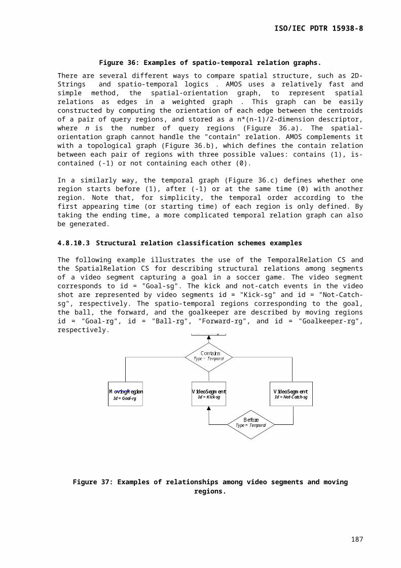
ISO/IEC PDTR 15938-8
;
}
Optimize the time instances of key-frames starting from the second key-frame positioned at as
follows. Determine ( ) by choosing that frame between and that produces the largest
value of the action measure with respect to the previous key-frame . This criterion can be referred to as the "largest successive difference" criterion.
A hierarchical key-frame summary is generated by clustering the key-frames extracted by the algorithm described above. Clustering is performed using the histogram vectors of key-frames. The clustering algorithm considers pairs of clusters of key-frames, where key-frames belonging to the
same cluster are consecutive in time. Let be the number of key-frames in the most detailed
summary of a particular shot. The next coarser level has key-frames, where is an arbitrary but predetermined compaction ratio. Start with an equally spaced partitioning of the key-frame histograms where each of the resulting partitions contains histogram vectors of consecutive key-frames (see Figure 43). Then, starting with the first partition, adjust each partition boundary between two adjacent partitions so as to minimize the l2 norm for the two adjacent partitions on either side of the partition boundary, as follows.
Assign the centroid histogram vector as the representative vector for each partition;
If is the representative vector for the vectors in the partition and is
the representative vector of the adjacent partition , adjust such that the total sum of squared distances of vectors in each cluster to the corresponding representative vector is minimized (see Figure 43).
If , then delete from the representative set of vectors. If , then
delete from the set of representative vectors.
Continue with the next pair of partitions, until all partition boundaries are processed.
Apply steps 1-4 for 10 iterations (or until the decrease in total distortion is insignificant). After stopping, the frame in the first cluster whose histogram vector is closest to the representative vector is selected as the first key-frame. Key-frames for subsequent clusters are determined according to the "largest successive difference" criterion expressed in terms of the action measure. Coarser level summaries can be obtained by recursive application of the above procedure.
(a) (b) (c)
Figure 43: Pairwise clustering for hierarchical key-frames summarization. In this example, the compaction ratio is 3. First T1 is adjusted in (a) considering only the two consecutive partitions
at either side of T1. Then T2 and T3 are adjusted as depicted in (b) and (c), respectively.
189

ISO/IEC PDTR 15938-8
Fidelity
The following algorithm describes computation of fidelity values associated with key-frames in a hierarchical key-frame summary. Assume that a feature descriptor such as a color histogram is available for each key-frame. Define a distance metric on the color histograms such as the l1 norm. Consider a hierarchical summary with key-frames as shown in Figure 44. The key-frame in each node is identified by A, B, etc., while fidelity values are denoted by e1, e2, etc. Consider, for example, the fidelity value e1, which indicates how well the key-frames in the subtree with root at node B is represented by the key-frame at node A. The fidelity value e1 can be obtained as follows.
Compute the maximum distance between the histogram of A and those of its children B, E, F and G;
Take the reciprocal of this maximum distance.
After all fidelity values in the hierarchy are computed, normalize them so that the fidelity values lie between 0.0 and 1.0.
Figure 44: An example of a key-frame hierarchy.
4.10.2.3.3 HierarchicalSummary DS use
In general, HierarchicalSummary descriptions can be used for navigation and browsing (e.g. visual table of contents or visual index of events), for viewing summarized content (e.g. visual highlights), and for scalable content viewing (e.g. adaptive to client or terminal capabilities and user preferences).
In the following, a method is described for utilizing the fidelity attribute of a HierarchicalSummary description. The notion of fidelity allows a variety of practically useful functionalities such as fidelity-based summary, scalable hierarchical summary and quick search. For example, if a user specifies a preferred number of key-frames to preview the whole video, then the system utilizes the fidelity attributes in the summary to select a given number of key-frames which best represent the original video in a sense defined by the encoder used to automatically generate the key-frame hierarchy. A set of key-frames are then sent to the terminal device for display.
Consider a key-frame hierarchy in Figure 44. In this example, key-frame B has three fidelity values e4, e5 and e6 associated with each of its three subtrees. The value e4 indicates the degree of representativeness of key-frame B over its subtree rooted at E. Thus, key-frame B represents its children contained in the subtree rooted at E with fidelity e4. As one goes down to finer levels, the fidelity values generally become larger, indicating that a key-frame at a finer level represents its subtree better than those at coarse levels. The following algorithm automatically selects a given number of key-frames from a key-frame hierarchy, based on the fidelity values. Denote the desired number of key-frames to be selected by N. Denote the set of key-frames with maximum fidelity by K.
initialize K to the empty set;
add the root node to K;
190

ISO/IEC PDTR 15938-8
WHILE ( card(K) < N ) {
consider nodes with a parent node such that ÎK and ÏK;
let be the node among these nodes with lowest fidelity value;
add to K;
}
The algorithm above yields the set K that contains the N key frames selected. For example, Figure 44, assume that N=2. If e3 is the minimum among e1, e2 and e3, the key frames A and D are selected. This decomposes the original tree in Figure 44 into the two subtrees shown in Figure 45.
Figure 45: An example of the key-frame selection algorithm based on fidelity values.
4.10.2.4 SummaryThemeList DS
4.10.2.4.1 SummaryThemeList DS examples
The following is an example of a SummaryThemeList, which contains a set of themes (e.g., certain kinds of events) for a sports news program. Note that this example describes a tree-structured representation of summary themes, as indicated by the parentID attributes. This structure is similar to an index and captures the themes in the multimedia content, allowing users to navigate the content accordingly. As shown in the last theme of the example ("John's favorite scenes"), a theme can be user-specific.
<SummaryThemeList><SummaryTheme xml:lang="en" id="item0"> baseball </SummaryTheme><SummaryTheme xml:lang="en" id="item01" parentID="item0">
home run </SummaryTheme><SummaryTheme xml:lang="en" id="item1"> basketball </SummaryTheme><SummaryTheme xml:lang="en" id="item11" parentID="item1">
three-pointer </SummaryTheme><SummaryTheme xml:lang="en" id="item12" parentID="item1">
slam dunk </SummaryTheme><SummaryTheme xml:lang="en" id="item2"> soccer </SummaryTheme><SummaryTheme xml:lang="en" id="item3"> John's favorite scenes
</SummaryTheme></SummaryThemeList>
191

ISO/IEC PDTR 15938-8
4.10.2.5 SummarySegmentGroup DS
4.10.2.5.1 SummarySegmentGroup DS examples
The following is an example of a set of two video summaries referring to particular events in a program, in particular "slam dunks" and "three-point shots" in a basketball game video. This description corresponds to the diagram shown in Figure 42. The first summary contains four video clips, each showing a slam dunk; the second summary contains three video clips, each showing a three-point shot. By grouping the clips into summaries of events, a user may choose to view only the clips of slam dunks; alternatively, the user may view all three-point shots. Note that in this case, there is no notion of hierarchy in the underlying real-world events.
<HierarchicalSummary components="keyVideoClips keyThemes" hierarchy="independent">
<SourceInformation idref="mediainstance1"/><SummaryThemeList>
<SummaryTheme xml:lang="en" id="E0"> slam dunk </SummaryTheme><SummaryTheme xml:lang="en" id="E1"> 3-point shot </SummaryTheme>
</SummaryThemeList><SummarySegmentGroup id="summary001" themeIDs="E0">
<Name>Slam dunks</Name><Caption>The L.A. Lakers scored four slam dunks in the second
half.</Caption><SummarySegment> <!-- segment #1 with slam dunk -->
</SummarySegment><SummarySegment> <!-- segment #2 with slam dunk -->
</SummarySegment><SummarySegment> <!-- segment #3 with slam dunk -->
</SummarySegment><SummarySegment> <!-- segment #4 with slam dunk -->
</SummarySegment></SummarySegmentGroup><SummarySegmentGroup id="summary002" themeIDs="E1">
<Name>3-Point shots</Name><Caption>The L.A. Lakers scored three 3-point shots in this
game.</Caption><SummarySegment> <!-- segment #1 with 3-pt shot -->
</SummarySegment><SummarySegment> <!-- segment #2 with 3-pt shot -->
</SummarySegment><SummarySegment> <!-- segment #3 with 3-pt shot -->
</SummarySegment></SummarySegmentGroup>
</HierarchicalSummary>
The following is an example of a hierarchical video summary consisting of a set of video clips organized into two levels. At the top level (i.e., level 0), the summary has a duration of 40 seconds and consists of only two video clips. At the second level (i.e., level 1), the summary has a duration of 100 seconds and consists of five video clips. Note that the coarse and the fine summary share two video clips, but these common clips are specified only once, by utilizing a dependent hierarchical structure (hierarchy is "dependent").
<HierarchicalSummary components="keyVideoClips" hierarchy="dependent"><SourceInformation idref="program001"/><SummarySegmentGroup id="highlight001" level="0" duration="PT40S">
<SummarySegment> <!-- segment #1 at level 0 --> </SummarySegment><SummarySegment> <!-- segment #2 at level 0 --> </SummarySegment><SummarySegmentGroup id="highlight002" level="1" duration="PT1M40S">
<SummarySegment> <!-- segment #1 at level 1 --> </SummarySegment>
192

ISO/IEC PDTR 15938-8
<SummarySegment> <!-- segment #2 at level 1 --> </SummarySegment>
<SummarySegment> <!-- segment #3 at level 1 --> </SummarySegment>
</SummarySegmentGroup></SummarySegmentGroup>
</HierarchicalSummary>
4.10.2.6 SummarySegment DS
4.10.2.6.1 SummarySegment DS examples
The HierarchicalSummary DS structures information in multimedia content into groups of video clips, audio clips, key frames and key sounds, possibly using a hierarchical set of levels. The resulting description allows navigating content by "zooming in" and "zooming out" to various levels of detail.
Figure 46 shows an example of a hierarchical key frame summary containing three levels. The key frame in each node is identified by A, B, and so forth, while fidelity values are denoted by e1, e2, and so forth. For example, the fidelity value e1 indicates how well the key frames in the subtree with root at node B is represented by the key frame at node A.
Figure 46: An example of a key-frame hierarchy.The following is a description of the key-frame hierarchy in Figure 46 using the HierarchicalSummary DS. Note that children SummarySegmentGroup elements are specified after SummarySegment elements at each node in the hierarchy. The fidelity values refer to Figure46 and should be understood as example values. Note that a summary consisting of key frames at a particular level of detail shall be constructed by combining information from all SummarySegmentGroup nodes at the same depth in a single tree. In this example, the most detailed summary is constructed by combining the key frames from all leaf (level 2) SummarySegmentGroup nodes.
<HierarchicalSummary components="keyFrames" hierarchy="independent"><SourceInformation idref="segment001"/><SummarySegmentGroup level="0" numOfKeyFrames="1">
<SummarySegment id="key_frame_A"><KeyFrame><MediaTimePoint>T00:06:45</MediaTimePoint></KeyFrame>
</SummarySegment>
<SummarySegmentGroup level="1"numOfKeyFrames="1" fidelity="0.4"> <!-- e1 --><SummarySegment id="key_frame_B">
<KeyFrame><MediaTimePoint>T00:03:45</MediaTimePoint></KeyFrame>
193

ISO/IEC PDTR 15938-8
</SummarySegment><SummarySegmentGroup level="2"
numOfKeyFrames="1" fidelity="0.4"> <!-- e4 --><SummarySegment id="key_frame_E">
<KeyFrame><MediaTimePoint>T00:02:00</MediaTimePoint> </KeyFrame>
</SummarySegment></SummarySegmentGroup><SummarySegmentGroup level="2"
numOfKeyFrames="1" fidelity="0.2"> <!-- e5 --><SummarySegment id="key_frame_F">
<KeyFrame><MediaTimePoint>T00:03:00</MediaTimePoint></KeyFrame>
</SummarySegment></SummarySegmentGroup><SummarySegmentGroup level="2"
numOfKeyFrames="1" fidelity="0.6"> <!-- e6 --><SummarySegment id="key_frame_G">
<KeyFrame><MediaTimePoint>T00:04:00</MediaTimePoint> </KeyFrame>
</SummarySegment></SummarySegmentGroup>
</SummarySegmentGroup>
<SummarySegmentGroup level="1" numOfKeyFrames="1" fidelity="0.5"> <!-- e2 --><SummarySegment id="key_frame_C">
<KeyFrame><MediaTimePoint>T00:07:15</MediaTimePoint></KeyFrame></SummarySegment><SummarySegmentGroup level="2"
numOfKeyFrames="1" fidelity="0.3"> <!-- e7 --><SummarySegment id="key_frame_H">
<KeyFrame><MediaTimePoint>T00:06:00</MediaTimePoint></KeyFrame>
</SummarySegment></SummarySegmentGroup><SummarySegmentGroup level="2"
numOfKeyFrames="1" fidelity="0.3"> <!-- e8 --><SummarySegment id="key_frame_I">
<KeyFrame><MediaTimePoint>T00:07:00</MediaTimePoint> </KeyFrame>
</SummarySegment></SummarySegmentGroup><SummarySegmentGroup level="2"
numOfKeyFrames="1" fidelity="0.8"> <!-- e9 --><SummarySegment id="key_frame_J">
<KeyFrame><MediaTimePoint>T00:08:00</MediaTimePoint></KeyFrame>
</SummarySegment></SummarySegmentGroup>
</SummarySegmentGroup>
<SummarySegmentGroup level="1" numOfKeyFrames="1" fidelity="0.2"> <!-- e3 --><SummarySegment id="key_frame_D">
<KeyFrame><MediaTimePoint>T00:10:40</MediaTimePoint></KeyFrame></SummarySegment><SummarySegmentGroup level="2"
numOfKeyFrames="1" fidelity="0.3"> <!-- e10 -->
194

ISO/IEC PDTR 15938-8
<SummarySegment id="key_frame_K"><KeyFrame><MediaTimePoint>T00:10:00</MediaTimePoint></KeyFrame>
</SummarySegment></SummarySegmentGroup><SummarySegmentGroup level="2"
numOfKeyFrames="1" fidelity="0.4"> <!-- e11 --><SummarySegment id="key_frame_L">
<KeyFrame><MediaTimePoint>T00:11:00</MediaTimePoint></KeyFrame>
</SummarySegment></SummarySegmentGroup><SummarySegmentGroup level="2"
numOfKeyFrames="1" fidelity="0.1"> <!-- e12 --><SummarySegment id="key_frame_M">
<KeyFrame><MediaTimePoint>T00:12:00</MediaTimePoint> </KeyFrame>
</SummarySegment></SummarySegmentGroup>
</SummarySegmentGroup></SummarySegmentGroup>
</HierarchicalSummary>
The fidelity values of the SummarySegmentGroup elements in a hierarchical summary may be used by an application to adaptively select SummarySegmentGroup elements. For instance, a variable number of key frames can be extracted from the HierarchicalSummary in a scalable manner, given fidelity values for all elements with key frames in the hierarchy.
4.10.2.7 SequentialSummary DS
4.10.2.7.1 SequentialSummary DS examples
Using the SequentialSummary DS, a sequence of images, or frames from a video program can be shown sequentially in time - for example, as an animated slide show. The SequentialSummary DS also supports fast playback of parts of a video program, by referring to a separately stored composite summary of video frames. The following example of a video summary illustrates the SequentialSummary DS. The first locator specifies the location of the original (source) video, while the second locator specifies the location of a composite video summary. Then, each VisualSummaryComponent element describes the properties of a particular frame in the original video.
<SequentialSummary id="SoccerSummary001" components="visual"><SourceLocator> <!-- source video -->
<MediaUri>file://disk/soccer/source/soccer001.mpg</MediaUri></SourceLocator><VideoSummaryLocator> <!-- summary video -->
<MediaUri>file://disk/soccer/summary/soccer001-summary.mpg</MediaUri></VideoSummaryLocator><VisualSummaryComponent> <!-- video frame #1 -->
</VisualSummaryComponent><VisualSummaryComponent> <!-- video frame #2 -->
</VisualSummaryComponent><VisualSummaryComponent> <!-- video frame #3 -->
</VisualSummaryComponent><VisualSummaryComponent> <!-- video frame #4 -->
</VisualSummaryComponent></SequentialSummary>
195

ISO/IEC PDTR 15938-8
Another example is illustrated in Figure 47, containing three tracks of elements associated with the multimedia content: image frames, textual annotation and audio clips. Each image frame is described by the VisualSummaryComponent D, each annotation is described by the TextualSummaryComponent D and each audio clip is described by the AudioSummaryComponent D.
Figure 47: Illustration of SequentialSummary DS.The following description corresponds to the diagram shown in Figure 47. Note that the components attribute enables applications to quickly identify the type of summary and the data contained therein.
<SequentialSummary id="SoccerSummary005" components="visual audio textual"><SourceLocator> <!-- source video -->
<MediaUri>file://disk/soccer/source/soccer001.mpg</MediaUri></SourceLocator><VisualSummaryComponent> <!-- video frame #1 -->
</VisualSummaryComponent><VisualSummaryComponent> <!-- video frame #2 -->
</VisualSummaryComponent><VisualSummaryComponent> <!-- video frame #3 -->
</VisualSummaryComponent><AudioSummaryComponent> <!-- video frame #4 -->
</AudioSummaryComponent><AudioSummaryComponent> <!-- audio clip #1 -->
</AudioSummaryComponent><AudioSummaryComponent> <!-- audio clip #2 -->
</AudioSummaryComponent><TextualSummaryComponent> <!-- text annotation #1 -->
</TextualSummaryComponent><TextualSummaryComponent> <!-- text annotation #2 -->
</TextualSummaryComponent></SequentialSummary>
196

ISO/IEC PDTR 15938-8
4.10.2.7.2 SequentialSummary DS extraction
In general, SequentialSummary descriptions can be constructed manually or automatically. To construct a SequentialSummary description, key-frames and sound-clips are extracted, selected and composed into a summary. In addition, textual annotation may be added to the SequentialSummary description.
Key-frames
In the following, an algorithm is described for automatic key-frame extraction. Note that parts of this algorithm may also be used to create other types of summary descriptions. This algorithm consists of the following steps, illustrated in Figure 48 (see also and ).
Feature points are extracted from each frame and then Kalman filtering is used to track the feature points in the next frame. Feature points correspond to points which contain a significant amount of texture, such as corner points. Such points are good candidates for tracking. The algorithm used for the feature points extraction step has been developed by Kanade et al. The KLT software library, which is publicly available at http://vision.stanford.edu/~birch/klt/index.html, can be used to implement the feature points extraction step. Other feature point extraction algorithms can be used also. Since many feature points have to be tracked, a data association filter is required. The nearest neighbor filter is used within this algorithm. In order to validate the association, a texture descriptor, characterizing the neighborhood of the feature point, is used. A track at time k is defined as a sequence of feature points up to time k which have been associated with the same target. See Figure 49 for an illustration.
Shot boundaries are detected using an activity measure based on the rate of change in tracks. This activity measure depends on the number of terminated or initiated tracks, and is defined as the maximum between terminated and initiated tracks calculated as a percentage. The percentage of initiated tracks is the number of new tracks divided by the total number of tracks in the current frame, while the percentage of terminated tracks is the number of removed tracks divided by the total number of tracks in the previous frame.
For shot boundary detection, a video sequence is modeled as a set of successive stationary and nonstationary states of the activity measure. Significant events correspond to the stationary states, which are characterized by a constant or slowly time-varying activity change. On the other hand, shot boundaries correspond to an abrupt change (cut) or fast change (dissolve). Accordingly, the temporal segmentation algorithm should fulfill the following requirements: a) detection of abrupt changes or fast changes; b) detection of stationary segments.
For this purpose, a recursive temporal segmentation algorithm is used, which models the data as a succession of states represented as a Gaussian process. A change in the state corresponds to a change in the parameters of the process (mean m and variance s2). The following equations are used in order to update the process parameters:
where is the current activity change and is a coefficient acting as an attenuation factor. If
then a new Gaussian process is initialized, with mean equal to the current activity change and standard deviation set as a large value. Figure 50 shows the activity change and its representation as a model of succession of Gaussian processes. Short impulses correspond to short processes with high activity change (shot boundaries), while longer segments correspond to Gaussian processes representing significant events.
A representative key-frame is extracted from the stationary or weakly non-stationary states (flat or oblique parts of the activity measure). The frame in the middle of the flat or oblique part is selected as a key-frame. Such a choice would allow representing the state in a compact way. For instance, in the case of a state that is part of a
197
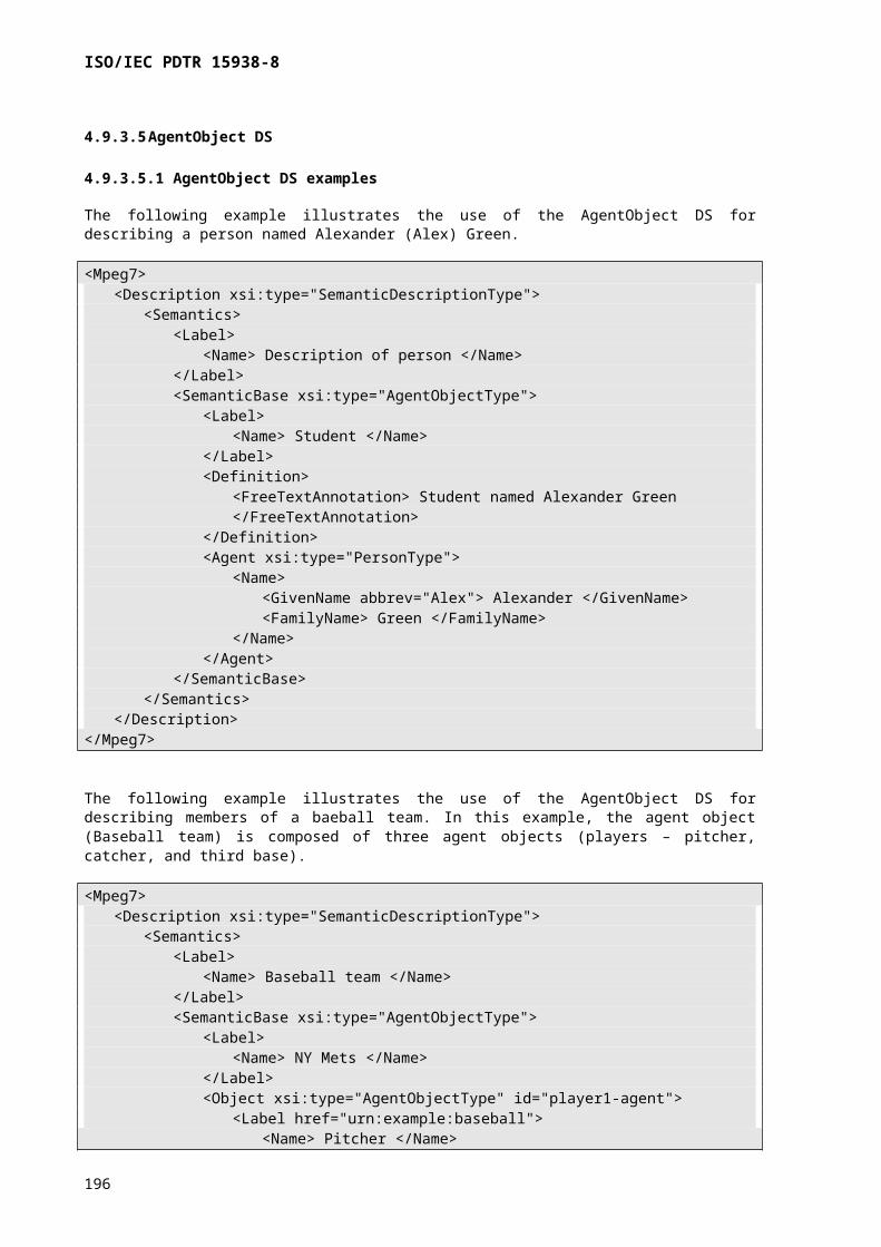
ISO/IEC PDTR 15938-8
zooming camera operation, the frame in the middle of this state is a good compromise between the wide and focused view.
A significant state corresponds to a state with a long duration or a high activity change value. The introduction of a significance value, computed as the product of the activity change value (activity change mean) and the duration of the corresponding state, allows us to have a scalable summary. The significance value, which is assigned to each key frame, could be interpreted as the surface of the rectangle built by the duration of the state and the activity change mean.
Once the key frames have been ordered according to their significance value, the number of key frames can be adapted according to the user’s preferences or the client device capabilities.
Figure 48: Shot boundary detection and key-frame selection.
Figure 49: Example tracking result (frame numbers 620, 621, 625). Note that many feature points disappear during the dissolve, while new feature points appear.
198

ISO/IEC PDTR 15938-8
Figure 50: Activity change (top). Segmented signal (bottom).
Frame-activity
In the following, a method is described for computing frame-activity values. Frame activity values are easily calculated from MPEG video streams because P-frames include information of motion vectors in macroblocks, from which frame-change-values can be computed, as follows.
Extract motion vectors from the inter coded macroblocks in a P-frame and sum up their absolute values.
Normalize the values with respect to the image size, by dividing the sum by the number of macroblocks in the frame.
Normalize the values based with respect to the time interval, by dividing the result of Step 2 by the duration between the P-frame and its reference picture.
The following are two special cases: the first is the case of intra coded macroblocks, and the second is the case of field predicted macroblocks. If a macroblock is intra coded, it is ignored. For the field-predicted macroblocks, multiply the absolute values of the motion vectors by 1/2 (because there are two motion vectors in the macroblock).
Note that a frame-change-value cannot be calculated from I- and B-frames. In order to calculate a frame-change-value for each frame, a linear approximation is used to interpolate missing values temporally. This procedure can be performed in a viewer application to decrease the size of the description. On the other hand, it is possible to calculate frame-change-values for all frames and include them in the description. In this case, viewer applications need no interpolation operation.
If the source video is not coded in MPEG-format, e.g. block-based template matching can be used to extract motion vectors. Another method for calculating frame-change-values is by applying pixel-wise
199
ISO/IEC PDTR 15938-8
subtraction of color values between one frame and the next frame. Using this method, almost the same effect can be obtained to implement smart quick view.
Thumbnails
Note that the video skim or smart quick view may consist of thumbnail-sizes images, to save data size. Thumbnails can be extracted from I-frames in an MPEG bitstream, by decoding only the DC DCT-coefficients of macroblocks. The size of the extracted images is 1/64th of the original. Each frame can be coded individually (such as a sequence of bitmaps, JPEG-images, etc.) or packed into one composite file (such as a Motion-JPEG file, QuickTime movie-file, etc.). When the thumbnails are saved in separate files, each ImageLocator element will contain a URL. On the other hand, when the thumbnails are packed into a single file, the location of the file is described by a URL in the VideoSummaryLocator element and each ImageLocator element contains only frame-numbers or time-stamps.
Thumbnail-sized images can also be obtained by selecting and decoding (if necessary) frames at some regular interval in a video stream, and down-sampling them into small size images. Note that smart quick view may require high-speed playback (without audio), in which case ready-made thumbnail-sized images are useful. However, in the case that frames from the original video stream are used, ready-made thumbnails are not required.
Regions-of-interest
In some applications, it is useful to indicate regions-of-interest in video images with varying sizes and from varying locations. For instance, the video content may contain frames with text or faces, which should be visualized at a higher resolution to highlight such areas or to improve readability of the video text, while other video data may be visualized at a lower resolution. In this case, the Region element may be used to specify such regions-of-interest in the original video frames. Also, the images in the video skim can be clipped from the corresponding original frames and stored separately as still images, which can be referred to using the ImageLocator element in the FrameProperty DS. The selection of such regions can be done manually, and should generally be adapted to the content. For instance, region-of-interests can be image regions with text, such as the score in a sports game, or regions with faces of persons that the user may be interested in. Note that there may be multiple regions-of-interest corresponding to the same video frame; this can be specified using multiple FrameProperty elements referring to the same frame (using the MediaTime element).
Audio-clips
In order to extract audio summary clips such as the main theme of popular song, the spectral characteristics of audio streams are analyzed. Analysis of time samples in the frequency domain is accompanied by time to frequency mapping, and many algorithms for this mapping exist. One of the flexible methods is that the input PCM samples are converted into subband samples by a filterbank, which is, for example, the method used in MPEG-1/-2 audio compression (Layers I and II). In case that the input audio format is MPEG audio, time to frequency mapping is not necessary, and the audio summary extraction algorithm described here can be directly applied to the subband data of the MPEG audio stream.
The audio clips corresponding to the main themes or clips including title phrases of popular songs can be regarded as audio summary clips. In general, these clips are emphasized and include relatively high level of music and/or vocal. This results in large subband energies for both music and vocal bands, or either. Consequently, a certain audio clip, which includes the maximum of sum of subband energy for music band and that for vocal band, can be extracted as the audio summary clip.
Then, the following steps are adopted in order to extract the audio summary.
Convert time samples into subband samples using the filterbank.
After the subband filtering, calculate the subband energy of each subband which is summed up for each second.
Calculate the summed subband energy for music band and that for vocal band at time T [second], according to the predefined band partition.
200

ISO/IEC PDTR 15938-8
Determine the start time of audio summary clip Tsummary according to the following criterion.
In this expression, denotes subband energy of base subband (subband zero), which
greatly relates to both music and vocal. , , and denote weighting factors for subband energies of music, vocal, and base respectively.
Once the start time of audio summary Tsummary is determined, assign the fixed time duration (according to the given duration constraint) or the time duration determined by another criterion, to each clip in order to compose audio summaries.
Composition of summaries with key-frames, audio-clips and textual annotation
To compose "slide-show" or "moving storyboard" summaries with key-frames, audio-clips and textual annotation, the following algorithms may be used.
Shot boundary and key-frame detection. Shot boundary detection is applied to the original video track, and the duration of every shot is recorded. Extract one key-frame per shot and use a FrameProperty element to describe each key-frame. Use the SyncTime element of each FrameProperty element to specify that the duration (intended display time) of the key-frame is that of the corresponding shot.
Time scale modification. A time scale modification algorithm can be used to speed up or slow down the audio by a factor, say N, preserving pitch and timbre. Hence the duration of the modified audio is N*d0, where d0 = duration of original audio. Modify the display time of each key-frame accordingly.
Speech recognition and information retrieval. Speech recognition can be used to detect terms. Key terms can be matched to a speech transcript for automatic labeling of the summary with key topics. Use TextProperty elements to specify and synchronize this textual annotation with the key-frames and audio-clips.
4.10.2.7.3 SequentialSummary DS use
In general, SequentialSummary descriptions can be used for rendering audio skims, video skims, or audio-visual slideshows.
In the following, a method is described for utilizing the FrameActivity element of FrameProperty elements in a SequentialSummary description. The SequentialSummary DS can be used to specify a video skim, similar to a fast forward video playback. The SequentialSummary DS also allows video playback with variable speed, also called "smart quick view". In conventional fast forward mode, video is played back at constant speed, independent of the amount of activity in the scene or scene motion, which can make it difficult to understand the video content. In smart quick view mode, video playback speed is adjusted so as to stabilize the amount of scene change. This requires computation of the amount of scene change for frames of the video. In this case, one of the frame-properties consists of the "frame-change-value", which is a measure of change from one frame to the next. Consequently, a viewer can dynamically adjust the playback frame rate. That is, playback speed is decreased if the frame-change-value is high and increased if it is low.
The following notation is used to describe normal quick view and smart quick view.
Frame rate of the original video: R frames/sec
Frame number of original video: i (0, 1, 2, …, K)
Frame-change-value for frame i: f(i)
Playback speed factor with respect to the original video frame rate: m
201

ISO/IEC PDTR 15938-8
Display frame rate (playback frame rate): r frames/sec
Display cycle number: j (0, 1, 2, …, N)
In the case of normal quick view, for each display cycle j (j=0,1,2,…,N), the frame number in the original video i is given by: (m*R/r)*j. The total number of displayed frames N is calculated by K/(m*R/r). Frame i can be extracted from the original video or a thumbnail-sized image may be used. In the case where a viewer application can only use I-frames of the original video, the I-frame nearest to the computed frame i can be used for display.
In the case of smart quick view, the frame-change-values are used to adjust playback speed automatically. Assume that frame-change-values f(i) are available for each frame i of the original video. If f(i) is not available for each frame, linear interpolation should be applied to compute the missing values. The frame-change-values f(i) are normalized such that their summation equals 1. Denote the normalized values by w(i), ( i=0,…, K-1). In order to stabilize playback in smart quick view mode and achieve the display frame rate r on average at the same time, the frame i to be displayed is controlled by the viewer based on w(i). Figure 51 shows a plot of the normalized frame-change-values w(i). The temporal axis can be partitioned into N segments, such that the sum of the frame-change-values w(i) inside each segment (approximately the area under the curve) equals 1/N. The boundaries between these segments are used as decision points to calculate the frame number i of the original video to be displayed, as follows. For display cycle j (the display frame rate is r), find the first i for
which . That is, accumulate the values of w(i) until their sum exceeds j/N. This determines the frame number i of the original video to be displayed at time j. Again, the nearest I-frame can be used if other frames are not available.
Figure 51: Illustration of smart quick view.
Another functionality of the SequentialSummary DS is to visualize a video containing various regions-of-interest. Such regions-of-interest may be zoomed into or highlighted by the viewer application. Or, such regions-of-interest may be used to synthesize images composed of thumbnails with different resolutions. In the latter case, the thumbnail images are given by a sequence of still images with arbitrary size. The size of the thumbnail image and its location in the original frame is chosen according to the video content. Note that more than one thumbnail image can correspond to the same original video frame. Thumbnail images corresponding to different regions in the same frame are layered to synthesize a single frame for visualization (see Figure 52).
Figure 5: Flowchart of "smart quick view"202

ISO/IEC PDTR 15938-8
Figure 52: Synthesizing frames in a video skim from multiple regions-of-interest.
4.10.2.8 VisualSummaryComponent D
4.10.2.8.1 VisualSummaryComponent D examples
The following is an example of a SequentialSummary, enabling a smart quick view, which is a variable speed presentation of the video content that uses the scene activity within parts of the original content to control the speed of summary presentation. In this instance, I-frames from the source video are included in the summary. However, scene activity is computed for P-frames from the source video. Each VisualSummaryComponent element in this summary contains a ComponentSourceTime element that refers to a frame in the original video with a number expressed in units of 1/30th of a second. Some VisualSummaryComponent elements also refer to the corresponding frame in the composite video summary using an ImageLocator element. Finally, some frames have a FrameActivity value associated with it, indicating the relative amount of activity in the original video. In this example, a single piece of original (source) data is being summarized; therefore, a single SourceLocator element in the SequentialSummary is sufficient.
<SequentialSummary id="SoccerSummary006" components="visual"><SourceLocator> <!-- Location of the source content -->
<MediaUri>file://disk/soccer/source/soccer001.mpg</MediaUri></SourceLocator><VideoSummaryLocator> <!-- Location of a composite video skim
summary -->
<MediaUri>file://disk/soccer/summary/soccer001-summary.mpg</MediaUri></VideoSummaryLocator>
<VisualSummaryComponent> <!-- Properties of video I-frame--><ComponentSourceTime> <!-- Frame number in the original video
--><MediaRelIncrTimePoint mediaTimeUnit="PT1N30F"
mediaTimeBase="../../../SourceLocator[1]">2</MediaRelIncrTimePoint>
</ComponentSourceTime><ImageLocator> <!-- Locates summary frame (in video
skim) --><MediaRelIncrTimePoint mediaTimeUnit="PT1N30F"
mediaTimeBase="../../../VideoSummaryLocator[1]">0</MediaRelIncrTimePoint>
</ImageLocator></VisualSummaryComponent>
<VisualSummaryComponent> <!-- Properties of video P-frame--><ComponentSourceTime> <!-- Frame number in the original video
--><MediaRelIncrTimePoint mediaTimeUnit="PT1N30F"
203
ISO/IEC PDTR 15938-8
mediaTimeBase="../../../SourceLocator[1]">5</MediaRelIncrTimePoint>
</ComponentSourceTime><FrameActivity>1.0</FrameActivity> <!-- Frame activity value -->
</VisualSummaryComponent>
<VisualSummaryComponent> <!-- Properties of video P-frame--><ComponentSourceTime> <!-- Frame number in the original video
--><MediaRelIncrTimePoint mediaTimeUnit="PT1N30F"
mediaTimeBase="../../../SourceLocator[1]">8</MediaRelIncrTimePoint>
</ComponentSourceTime><FrameActivity>0.9</FrameActivity> <!-- Frame activity value -->
</VisualSummaryComponent>
<VisualSummaryComponent> <!-- Properties of video I-frame--><ComponentSourceTime> <!-- Frame number in the original video
--><MediaRelIncrTimePoint mediaTimeUnit="PT1N30F"
mediaTimeBase="../../../SourceLocator[1]">11</MediaRelIncrTimePoint>
</ComponentSourceTime><ImageLocator> <!-- Locates summary frame (in video
skim) --><MediaRelIncrTimePoint mediaTimeUnit="PT1N30F"
mediaTimeBase="../../../VideoSummaryLocator[1]">1</MediaRelIncrTimePoint>
</ImageLocator></VisualSummaryComponent>
<VisualSummaryComponent> <!-- Properties of video P-frame--><ComponentSourceTime> <!-- Frame number in the original video
--><MediaRelIncrTimePoint mediaTimeUnit="PT1N30F"
mediaTimeBase="../../../SourceLocator[1]">14</MediaRelIncrTimePoint>
</ComponentSourceTime><FrameActivity>0.8</FrameActivity> <!-- Frame activity value -->
</VisualSummaryComponent>
<VisualSummaryComponent> <!-- Properties of video P-frame--><ComponentSourceTime> <!-- Frame number in the original video
--><MediaRelIncrTimePoint mediaTimeUnit="PT1N30F"
mediaTimeBase="../../../SourceLocator[1]">17</MediaRelIncrTimePoint>
</ComponentSourceTime><FrameActivity>0.5</FrameActivity> <!-- Frame activity value -->
</VisualSummaryComponent>
<VisualSummaryComponent> <!-- Properties of video I-frame--><ComponentSourceTime> <!-- Frame number in the original video
--><MediaRelIncrTimePoint mediaTimeUnit="PT1N30F"
mediaTimeBase="../../../SourceLocator[1]">20</MediaRelIncrTimePoint>
</ComponentSourceTime><ImageLocator> <!-- Locates summary frame (in video
skim) --><MediaRelIncrTimePoint mediaTimeUnit="PT1N30F"
204

ISO/IEC PDTR 15938-8
mediaTimeBase="../../../VideoSummaryLocator[1]">2</MediaRelIncrTimePoint>
</ImageLocator></VisualSummaryComponent>
</SequentialSummary>
4.10.2.9 AudioSummaryComponent D
4.10.2.9.1 AudioSummaryComponent D examples
The AudioSummaryComponent D can be used to provide an audio slide show (a succession of audio clips) and supports summarization of multiple pieces of content, such as a summary of multiple songs recorded on one CD album. In addition to playing audio slides (i.e., clips) one by one, applications can use the AudioSourceLocator element in order to switch playback between an audio slide component and its original. For example, one can listen to pieces of songs in the form of an audio slide show described by AudioSummaryComponent elements; and if one encounters some audio piece of his/her favorite song at a certain location in the song, one can listen to its original from that point forward.
There may be several types of audio summaries, depending on whether the original content is stored in a single stream of file, or in multiple streams or files. Also, each audio slide in the summary may be either: a) part of the original content, b) part of a composite summary, or c) in a separate stream or file.
The following figure illustrates the case when there is a single source, but each audio summary component (audio clip) is located in a separate audio clip file.
Figure 53: Example of an audio summary with a single source.In this case, the top-level SourceLocator associated with the entire summary indicates the location of a single source ("moz-req.aif"). AudioSourceLocator elements associated with each slide specify the location of audio clips (e.g. a song, a movement) using MediaTime elements (00m 00s to 05m 01s for the first part, and 05m 01s to 07m 41s for the second part). ComponentSourceTime elements indicate the start time and duration of audio summary components in the source, and SoundLocator elements each locate a separate audio clip using a MediaUri element ("Requiem.aif" and "Kyrie.aif" respectively).
<SequentialSummary id="classics004" components="audio"><Name>Mozart's Requiem KV 626</Name> <!-- Summary name --><SourceLocator> <!-- Location of the source content -->
<MediaUri>file://Mozart/moz-req.aif</MediaUri></SourceLocator>
<AudioSummaryComponent> <!-- Component #1 --><Title xml:lang="de">INTROITUS: Requiem</Title><AudioSourceLocator> <!-- Location of movement #1 within the
source --><MediaTime>
<MediaRelTimePoint mediaTimeBase="../../../../SourceLocator[1]">PT0S
205

ISO/IEC PDTR 15938-8
</MediaRelTimePoint><MediaDuration>PT05M01S</MediaDuration>
</MediaTime></AudioSourceLocator><ComponentSourceTime> <!-- Location of component #1 within the
source --><MediaRelTimePoint
mediaTimeBase="../../../SourceLocator[1]">PT0S</MediaRelTimePoint><MediaDuration>PT47S</MediaDuration>
</ComponentSourceTime><SoundLocator> <!-- File location of slide component #1 -->
<MediaUri>file://Mozart/Requiem.aif</MediaUri></SoundLocator>
</AudioSummaryComponent>
<AudioSummaryComponent> <!-- Component #2 --><Title xml:lang="de">KYRIE</Title><AudioSourceLocator> <!-- Location of movement #2 within the
source --><MediaTime>
<MediaRelTimePoint mediaTimeBase="../../../../SourceLocator[1]">PT05M01S
</MediaRelTimePoint><MediaDuration>PT02M40S</MediaDuration>
</MediaTime></AudioSourceLocator><ComponentSourceTime> <!-- Location of component #2 within the
source --><MediaRelTimePoint
mediaTimeBase="../../../SourceLocator[1]">PT05M01S</MediaRelTimePoint><MediaDuration>PT30S</MediaDuration>
</ComponentSourceTime><SoundLocator> <!-- File location of slide component #2 -->
<MediaUri>file://Mozart/Kyrie.aif</MediaUri></SoundLocator>
</AudioSummaryComponent>
<!-- More AudioSummaryComponent elements ... --></SequentialSummary>
The following figure illustrates the case when there are multiple sources, and the audio summary components (audio clips) are all part of a composite audio summary.
Figure 54: Example of an audio summary with multiple sources.In this case, the AudioSummaryLocator element locates the composite audio summary ("TWOTON.aif"). The AudioSourceLocator elements in each AudioSummaryComponent element
206

ISO/IEC PDTR 15938-8
specify the location of each source using MediaUri ("TWOTON-1.aif" and "TWOTON-2.aif", respectively). ComponentSourceTime elements refer to the location of the audio clips within the source, and SoundLocator elements indicate the start time and duration of the audio clips within the composite audio summary using MediaTime (00s to 09s, and 10s to 18s, respectively). The Title element indicates the song title.
<SequentialSummary id="rock007" components="audio"><Name>Two Ton Shoe Rock Album</Name> <!-- Summary name --><AudioSummaryLocator> <!-- Location of the composite audio summary
--><MediaUri>file://TwoTonShoe/Summary/TWOTON.aif</MediaUri>
</AudioSummaryLocator>
<AudioSummaryComponent> <!-- Component #1 --><Title xml:lang="en">Brothers</Title><AudioSourceLocator> <!-- Location of source #1 -->
<MediaUri>file://TwoTonShoe/TWOTON-1.aif</MediaUri></AudioSourceLocator><ComponentSourceTime> <!-- Location of component #1 within the
source --><MediaRelTimePoint
mediaTimeBase="../../AudioSourceLocator[1]">PT01M06S</MediaRelTimePoint><MediaDuration>PT09S</MediaDuration>
</ComponentSourceTime><SoundLocator> <!-- Location of component #1 within audio
summary --><MediaTime>
<MediaRelTimePointmediaTimeBase="../../../../AudioSummaryLocator[1]">PT0S
</MediaRelTimePoint><MediaDuration>PT09S</MediaDuration>
</MediaTime></SoundLocator>
</AudioSummaryComponent>
<AudioSummaryComponent> <!-- Component #2 --><Title xml:lang="en">Georgie</Title><AudioSourceLocator> <!-- Location of source #2 -->
<MediaUri>file://TwoTonShoe/TWOTON-2.aif</MediaUri></AudioSourceLocator><ComponentSourceTime> <!-- Location of component #2 within the
source --><MediaRelTimePoint
mediaTimeBase="../../AudioSourceLocator[1]">PT17S</MediaRelTimePoint><MediaDuration>PT08S</MediaDuration>
</ComponentSourceTime><SoundLocator> <!-- Location of component #2 within audio
summary --><MediaTime>
<MediaRelTimePoint mediaTimeBase="../../../../AudioSummaryLocator[1]">PT10S
</MediaRelTimePoint><MediaDuration>PT08S</MediaDuration>
</MediaTime></SoundLocator>
</AudioSummaryComponent>
<!-- More AudioSummaryComponent elements ... --></SequentialSummary>
207

ISO/IEC PDTR 15938-8
4.10.2.10 TextualSummaryComponent D
4.10.2.10.1TextualSummaryComponent D examples
The TextualSummaryComponent D can be used to synchronize text data with audio, video or audiovisual summaries. The following example shows the use of text to describe a table of contents of a presentation. The summary itself contains video frames, each associated with a particular video segment in the presentation, synchronized with a composite audio summary. Each video frame is stored in a separate (JPEG) file. For this example, start and end time of the video segments and their associated textual information in the summary video are as follows.
Topic Start Time End Time Duration
"Introduction" 00:00:00 00:01:00 1 min
"Business Model" 00:01:01 00:03:00 2 min
"Stock Options" 00:03:01 00:05:00 2 min
"Get Rich Quick" 00:05:01 00:06:00 1 min
<SequentialSummary id="MSB4" components="visual audio textual"><AudioSummaryLocator> <!-- Composite audio summary -->
<MediaUri>http://www.mywebsite.com/CueVideo/audio_summary001.mp3</MediaUri>
<MediaTime><MediaTimePoint>T00:00:00</MediaTimePoint><MediaDuration>PT6M</MediaDuration>
</MediaTime></AudioSummaryLocator>
<VisualSummaryComponent><ImageLocator> <!-- Locates summary frame #1 -->
<MediaUri>http://www.mywebsite.com/CueVideo/speaker1.jpg</MediaUri></ImageLocator> <!-- Duration of frame #1 in summary video: 1 min
--><SyncTime>
<MediaTimePoint>T00:00:00</MediaTimePoint><MediaDuration>PT01M</MediaDuration>
</SyncTime></VisualSummaryComponent><VisualSummaryComponent>
<ImageLocator> <!-- Locates summary frame #2 -->
<MediaUri>http://www.mywebsite.com/CueVideo/speaker2.jpg</MediaUri></ImageLocator> <!-- Duration of frame #2 in summary video: 4 min
--><SyncTime>
<MediaTimePoint>T00:01:00</MediaTimePoint><MediaDuration>PT04M</MediaDuration>
</SyncTime></VisualSummaryComponent><VisualSummaryComponent>
<ImageLocator> <!-- Locates summary frame #3 -->
208
ISO/IEC PDTR 15938-8
<MediaUri>http://www.mywebsite.com/CueVideo/speaker3.jpg</MediaUri></ImageLocator> <!-- Duration of frame #3 in summary video: 1 min
--><SyncTime>
<MediaTimePoint>T00:05:00</MediaTimePoint><MediaDuration>PT01M</MediaDuration>
</SyncTime></VisualSummaryComponent>
<TextualSummaryComponent><FreeText xml:lang="en"> Introduction </FreeText><SyncTime> <!-- Synchronizes text information with summary -->
<MediaTimePoint>T00:00:00</MediaTimePoint><MediaDuration>PT01M</MediaDuration>
</SyncTime></TextualSummaryComponent><TextualSummaryComponent>
<FreeText xml:lang="en"> Business Model </FreeText><SyncTime> <!-- Synchronizes text information with summary -->
<MediaTimePoint>T00:01:00</MediaTimePoint><MediaDuration>PT02M</MediaDuration>
</SyncTime></TextualSummaryComponent><TextualSummaryComponent>
<FreeText xml:lang="en"> Stock Options </FreeText><SyncTime> <!-- Synchronizes text information with summary -->
<MediaTimePoint>T00:03:00</MediaTimePoint><MediaDuration>PT02M</MediaDuration>
</SyncTime></TextualSummaryComponent><TextualSummaryComponent>
<FreeText xml:lang="en"> Get Rich Quick </FreeText><SyncTime> <!-- Synchronizes text information with summary -->
<MediaTimePoint>T00:05:00</MediaTimePoint><MediaDuration>PT01M</MediaDuration>
</SyncTime></TextualSummaryComponent>
</SequentialSummary>
4.10.3 Views, partitions and decompositions
4.10.3.1 Partition datatype
4.10.3.1.1 Partition datatype examples
The following examples illustrate descriptions of two-dimensional Partitions measured in samples and fractions. The first example specifies a two-dimensional partition, such as a partition of an image, which starts at sample or pixel (20, 40) and ends at sample (100, 100). This gives the Partition a size of (80 x 60) samples or pixels. The second example specifies a two-dimensional partition, which starts at position (0.0, 0.0) and has size (0.5, 0.5) relative to the size of the space. For example, in describing a Partition of a (512 x 512) image, the Partition would start at pixel position (0, 0) and have size (256, 256) samples or pixels.
<Partition><Origin xOrigin="left" yOrigin="top" /><Start xsi:type="SignalPlaneSampleType" x="20" y="40" /><End xsi:type="SignalPlaneSampleType" x="100" y="100" />
</Partition>
209

ISO/IEC PDTR 15938-8
<Partition dim="2"><Origin xOrigin="left" yOrigin="bottom" /><Start xsi:type="SignalPlaneFractionType" x="0.0" y="0.0" /><Extent xsi:type="SignalPlaneFractionType" x="0.5" y="0.5" />
</Partition>
4.10.3.2 Filter datatype
4.10.3.2.1 Filter datatype examples
The following example describes a 1-D discrete filter. The terms of the filter have values 0.5 and 0.5. The example defines a two-tap averaging filter, which when applied to audio takes the average of neighboring samples.
<Filter1D><Terms mpeg7:dim="2"> 0.5 0.5 </Terms>
</Filter1D>
The following example describes a 2-D discrete filter. The filter corresponds to a 3 x 3 Laplacian filter, which when applied to an image takes the difference of pixel values vertically and horizontally in the neighborhood around each pixel. The Laplacian filter is commonly used for edge detection.
<Filter2D><Terms mpeg7:dim="3 3">
0.0 -1.0 0.0 -1.0 4.0 -1.0 0.0 -1.0 0.0
</Terms></Filter2D>
The following example describes a discrete multi-dimensional separable filter. The individual filters that make up the separable filter are specified as two three-tap one-dimensional filters. The terms of the 2-D separable filter are derived from the direct product of the 1-D filters to produce the 2-D separable filter. The derived terms of the 2-D separable filter (top) are equivalent to those of the 2-D filter specified below it (bottom). The example defines a low-pass filter, which when applied to an image takes the average of neighboring samples.
<FilterSeparable><Filter1D><Terms mpeg7:dim="3"> 1.0 2.0 1.0 </Terms></Filter1D><Filter1D><Terms mpeg7:dim="3"> 1.0 2.0 1.0 </Terms></Filter1D>
</FilterSeparable>
<Filter2D><Terms mpeg7:dim="3 3">
1.0 2.0 1.0 2.0 4.0 2.0 1.0 2.0 1.0
</Terms></Filter2D>
210

ISO/IEC PDTR 15938-8
4.10.3.3 Filtering datatype
4.10.3.3.1 Filtering datatype examples
The following example describes the filtering of an image using a discrete 2-D filter. The description specifies the padding of the image by one pixel on each dimension using symmetric extension. The description also specifies the shifting of the filter kernel by one sample or pixel in both the horizontal and vertical direction before taking the convolution sum. The description also specifies the output image should be cropped by one pixel at all borders (left, top, right and bottom). The example uses a 2-D filter of size 3 x 3.
<Filtering xPad="symmetric" yPad="symmetric" ><Filter xsi:type="Filter2DType">
<Terms mpeg7:dim="3 3"> 1.0 2.0 1.0 2.0 4.0 2.0 1.0 2.0 1.0
</Terms></Filter><PadSize x="1" y="1" /><Shift x="1" y="1" /><CropStart x="1" y="1" /><CropEnd x="1" y="1" />
</Filtering>
4.10.3.4 View DS
4.10.3.4.1.1 View DS Use
Space and frequency views can be used in applications that involve the access and navigation of large images and video at multiple resolutions. For example, browsing applications of large aerial images and maps involve the interactive zooming-in, zooming-out and panning around the 2-D image data. Typically, each operation requires the extraction, delivery and/or synthesis, and display of a space and frequency view of the large image. A similar framework applies to the progressive delivery of video at multiple spatial and temporal resolutions.
4.10.3.5 SpaceView DS
4.10.3.5.1 SpaceView DS examples
The following examples describe different SpaceViews. The first example describes a SpaceView which corresponds to the upper-left quadrant of an image.
<Mpeg7><Description xsi:type="ViewDescriptionType">
<View xsi:type="SpaceViewType"><Target>
<ImageSignal><MediaLocator>
<MediaUri>file://Aerial-upperleft.jpg</MediaUri></MediaLocator>
</ImageSignal></Target><Source>
<ImageSignal><MediaLocator>
<MediaUri>file://Aerial.jpg</MediaUri></MediaLocator>
211

ISO/IEC PDTR 15938-8
</ImageSignal></Source><SpacePartition>
<Origin xOrigin="left" yOrigin="top"/><Start xsi:type="SignalPlaneFractionType" x="0" y="0"/><End xsi:type="SignalPlaneFractionType" x="0.5" y="0.5"/>
</SpacePartition></View>
</Description></Mpeg7>
The second example describes a SpaceView which corresponds to the first 16000 samples of an audio signal.
<Mpeg7><Description xsi:type="ViewDescriptionType">
<View xsi:type="SpaceViewType"><Target>
<AudioSignal><MediaLocator>
<MediaUri>music-intro.mp3</MediaUri></MediaLocator>
</AudioSignal></Target><Source>
<AudioSignal><MediaLocator>
<MediaUri>music.mp3</MediaUri></MediaLocator>
</AudioSignal></Source><SpacePartition>
<Start xsi:type="SignalPlaneSampleType" t="0"/><End xsi:type="SignalPlaneSampleType" t="16384"/>
</SpacePartition></View>
</Description></Mpeg7>
Examples of Space Views include regions of still images, temporal segments of video and temporal segments of audio. Figure 55.a) shows a large aerial image of which only a small subset depicting a rocky area is of interest to the user, see Figure 55.b). The Space View DS is used to describe this spatial view of the large 2-D image.
212

ISO/IEC PDTR 15938-8
(a) (b)
Figure 55: Aerial image (a) source: Aerial image LB_120.tif, and (b) a part of image a) based on a spatial view DS.
4.10.3.6 FrequencyView DS
4.10.3.6.1 FrequencyView DS examples
The following example describes a FrequencyView that corresponds to a twice-iterated, low-pass, low-pass wavelet subband of an audio signal. The FrequencyView corresponds to the first one-quarter of the frequency plane. Furthermore, the filtered signal is down-sampled by a factor of four to produce a Target FrequencyView audio signal that has one-quarter the number of samples as the Source audio signal. In practice, the example below specifies a coarse version of the audio signal.
<Mpeg7><Description xsi:type="ViewDescriptionType">
<View xsi:type="FrequencyViewType"><Target>
<AudioSignal><MediaLocator>
<MediaUri>file://audio-ll.mp3</MediaUri></MediaLocator>
</AudioSignal></Target><Source>
<AudioSignal><MediaLocator>
<MediaUri>file://audio.mp3</MediaUri></MediaLocator>
</AudioSignal></Source><FrequencyPartition>
<Start xsi:type="SignalPlaneFractionType" t="0"/><End xsi:type="SignalPlaneFractionType" t="0.25"/>
</FrequencyPartition><DownSamplingFactor t="4"/>
</View></Description>
</Mpeg7>
213

ISO/IEC PDTR 15938-8
In general, examples of Frequency Views include spatial-frequency subbands of still images, 3-D wavelet subbands of video and temporal-frequency subbands of audio. The sample below illustrates a frequency view of an aerial image, which corresponds to a spatial-frequency subband of the image.
Figure 56: Frequency View of an Aerial image – spatial-frequency subband.
4.10.3.7 SpaceFrequencyView DS
4.10.3.7.1 SpaceFrequencyView DS examples
The following example describes a SpaceFrequencyView that corresponds to a wavelet subband of a region of an image. The SpaceFrequencyView corresponds to the lower one-quarter of the spatial-frequency plane of the upper-left corner region of the image. Furthermore, the filtered region is down-sampled by a factor of two on each dimension to produce a Target SpaceFrequencyView image that has one-sixteenth the number of samples as the Source image. In this example, the order of the space and frequency analysis operations to extract the view is specified as space first then frequency. In practice, the example below specifies a coarse version of the upper-left region of the image.
<Mpeg7><Description xsi:type="ViewDescriptionType">
<View xsi:type="SpaceFrequencyViewType" order="spaceFrequency"><Target>
<ImageSignal><MediaLocator>
<MediaUri>file://soccer-ul-ll.jpg</MediaUri></MediaLocator>
</ImageSignal></Target><Source>
<ImageSignal><MediaLocator>
<MediaUri>file://soccer.jpg</MediaUri></MediaLocator>
</ImageSignal></Source><SpacePartition>
<Start xsi:type="SignalPlaneFractionType" x="0" y="0"/><End xsi:type="SignalPlaneFractionType" x="0.5" y="0.5"/>
</SpacePartition><FrequencyPartition>
<Start xsi:type="SignalPlaneFractionType" x="0" y="0"/><End xsi:type="SignalPlaneFractionType" x="0.5" y="0.5"/>
</FrequencyPartition><DownSamplingFactor x="2" y="2"/>
</View></Description>
214

ISO/IEC PDTR 15938-8
</Mpeg7>
4.10.3.7.1.1 SpaceFrequencyView DS Examples
Examples of Space Frequency Views include spatial-frequency subbands of regions of still images, 3-D wavelet subbands of temporal segments of video and temporal-frequency subbands of temporal segments of audio. An example of a Space Frequency View is given in Figure 57. The data of an aerial image is shown in some spatial region with all frequency components, in others only the lowband components are transmitted to provide some context information.
Figure 57: Example SpaceFrequency view of Figure 55 using a high resolution for the region of interest and a reduced resolution for the context
4.10.3.8 ResolutionView DS
4.10.3.8.1 ResolutionView DS examples
The following example describes a ResolutionView that corresponds a one-sixteenth size thumbnail view of an image (downsampled by a factor of four along both dimensions).
<Mpeg7><Description xsi:type="ViewDescriptionType">
<View xsi:type="ResolutionViewType"><Target>
<ImageSignal><MediaLocator>
<MediaUri>file://soccer-coarse.jpg</MediaUri></MediaLocator>
</ImageSignal></Target><Source>
<ImageSignal><MediaLocator>
<MediaUri>file://soccer.jpg</MediaUri></MediaLocator>
</ImageSignal></Source><DownSamplingFactor x="4" y="4"/>
</View>
215

ISO/IEC PDTR 15938-8
</Description></Mpeg7>
Examples of Space Resolution Views include subsampled spatial-frequency subbands of regions of still images, 3-D wavelet subbands of temporal segments of video and temporal-frequency subbands of temporal segments of audio. Often it is only necessary to access an overview or low-resolution version of a large image. In this case, it is sufficient to look at the representation of an image generated by the low frequency components of the image. For this purpose the view can be described by a ResolutionView DS or, more generally by a FrequencyView DS. The ResolutionView DS describes the reduction of the image using low pass filtering. For example, Figure 58shows a low-resolution view of a large aerial image.
Figure 58: Example view of image with reduced resolution.
4.10.3.8.2 ResolutionView DS extraction
A Resolution View can be extracted from an image, video, or audio signal by sub-setting the data and by using a low-pass filter that in the Fourier domain corresponds to a low-frequency partition of the sub-set in the frequency plane.
4.10.3.9 SpaceResolutionView DS
4.10.3.9.1 SpaceResolutionView DS examples
The following example describes a SpaceResolutionView that corresponds to a coarse or thumbnail view of a region of an image. The SpaceResolutionView corresponds to the lower one-quarter resolution view of the upper-left corner region of the image. In this example, the order of the space and frequency (resolution) analysis operations to extract the view is specified as space first then frequency (resolution).
<Mpeg7><Description xsi:type="ViewDescriptionType">
<View xsi:type="SpaceResolutionViewType" order="spaceFrequency"><Target>
<ImageSignal><MediaLocator>
<MediaUri>file://soccer-ul-ll.jpg</MediaUri></MediaLocator>
</ImageSignal></Target><Source>
<ImageSignal><MediaLocator>
<MediaUri>file://soccer.jpg</MediaUri></MediaLocator>
</ImageSignal></Source><SpacePartition>
<Start xsi:type="SignalPlaneFractionType" x="0" y="0"/><End xsi:type="SignalPlaneFractionType" x="0.5" y="0.5"/>
</SpacePartition><DownSamplingFactor x="2" y="2"/>
216
ISO/IEC PDTR 15938-8
</View></Description>
</Mpeg7>
Figure 59.a) shows a large aerial image of which only a small subset depicting a rocky area is of interest to the user, see Figure 59.b). The SpaceResolution View DS is used to describe this view of the large 2-D image.
(a) (b)
Figure 59: Aerial image (a) source: Aerial image LB_120.tif, and (b) a part of image a) based on a spatial view DS.
4.10.3.10 ViewDecomposition DS
4.10.3.11 ViewSet DS
4.10.3.11.1ViewSet DS examples
The following example describes a ViewSet that contains two SpaceViews. The ViewSet is specified to be nonredundant and not complete. In this example, the two views correspond to the upper-left and upper-right quadrants, respectively, of the source image specified as the source of the view set. In both cases, the specification of the SpacePartition is given in relation to the source image of the view set.
<Mpeg7><Description xsi:type="ViewDescriptionType">
<ViewSet complete="false" nonRedundant="true" setProperty="space"><Source>
<ImageSignal><MediaLocator>
<MediaUri>file://soccer.jpg</MediaUri></MediaLocator>
</ImageSignal></Source><View xsi:type="SpaceViewType">
<Target><ImageSignal>
<MediaLocator><MediaUri>file://soccer-upper-left.jpg</MediaUri>
</MediaLocator></ImageSignal>
</Target>
217
ISO/IEC PDTR 15938-8
<SpacePartition><Start xsi:type="SignalPlaneFractionType" x="0" y="0"/><End xsi:type="SignalPlaneFractionType" x="0.5" y="0.5"/>
</SpacePartition></View><View xsi:type="SpaceViewType">
<Target><ImageSignal>
<MediaLocator><MediaUri>file://soccer-upper-right.jpg </MediaUri>
</MediaLocator></ImageSignal>
</Target><SpacePartition>
<Start xsi:type="SignalPlaneFractionType" x="0.5" y="0"/><End xsi:type="SignalPlaneFractionType" x="1.0" y="0.5"/>
</SpacePartition></View>
</ViewSet></Description>
</Mpeg7>
Examples of View Sets include a set of spatial-frequency subbands of an image and a set of layers of scalable video data.
Figure 60: Example View Set with a set of Frequency Views that are image subbands. This View Set is complete and nonredundant.
4.10.3.12 SpaceTree DS
4.10.3.12.1SpaceTree DS examples
The following example describes a SpaceTree with branching factor of two at the root node, which corresponds to the splitting of the source image into two child space views. The specification of the SpacePartitions of the Child views is given in relation to the Source image of the SpaceTree.
<Mpeg7><Description xsi:type="ViewDescriptionType">
<ViewDecomposition xsi:type="SpaceTreeType" complete="false" nonRedundant="true" branching="2">
218

ISO/IEC PDTR 15938-8
<Source><ImageSignal>
<MediaLocator><MediaUri>soccer.jpg</MediaUri>
</MediaLocator></ImageSignal>
</Source><Child branching="0">
<View><Target>
<ImageSignal><MediaLocator>
<MediaUri>soccer-00.jpg</MediaUri></MediaLocator>
</ImageSignal></Target><SpacePartition>
<Start xsi:type="SignalPlaneFractionType" x="0.0" y="0"/>
<End xsi:type="SignalPlaneFractionType" x="0.5" y="0.5"/>
</SpacePartition></View>
</Child><Child branching="0">
<View><Target>
<ImageSignal><MediaLocator>
<MediaUri>soccer-01.jpg</MediaUri></MediaLocator>
</ImageSignal></Target><SpacePartition>
<Start xsi:type="SignalPlaneFractionType" x="0.5" y="0"/>
<End xsi:type="SignalPlaneFractionType" x="1.0" y="0.5"/>
</SpacePartition></View>
</Child></ViewDecomposition>
</Description></Mpeg7>
4.10.3.13 FrequencyTree DS
4.10.3.13.1FrequencyTree DS examples
The following example describes a FrequencyTree with branching factor of two at the root node. The FrequencyTree specifies one FrequencyView at the first level of the tree and two FrequencyView at the second level of the tree.
<Mpeg7><Description xsi:type="ViewDescriptionType">
<ViewDecomposition xsi:type="FrequencyTreeType" complete="false" nonRedundant="true" branching="2"><Source>
<ImageSignal>
219

ISO/IEC PDTR 15938-8
<MediaLocator><MediaUri>soccer.jpg</MediaUri>
</MediaLocator></ImageSignal>
</Source><Child branching="0">
<View><Target>
<ImageSignal><MediaLocator>
<MediaUri>soccer-ll.jpg</MediaUri></MediaLocator>
</ImageSignal></Target><FrequencyPartition>
<Start xsi:type="SignalPlaneFractionType" x="0" y="0"/><End xsi:type="SignalPlaneFractionType" x="0.5"
y="0.5"/></FrequencyPartition>
</View></Child><Child branching="0">
<View><Target>
<ImageSignal><MediaLocator>
<MediaUri>soccer-lh.jpg</MediaUri></MediaLocator>
</ImageSignal></Target><FrequencyPartition>
<Start xsi:type="SignalPlaneFractionType" x="0" y="0.5"/>
<End xsi:type="SignalPlaneFractionType" x="0.5" y="1"/></FrequencyPartition>
</View></Child>
</ViewDecomposition></Description>
</Mpeg7>
4.10.3.14 SpaceFrequencyGraph DS
4.10.3.14.1SpaceFrequencyGraph DS examples
The following example describes a SpaceFrequencyGraph with branching factor of two on each space and frequency dimension at the root node. The SpaceFrequencyGraph specifies one SpaceFrequencyView at the first level of the directed acyclic graph and four SpaceFrequencyViews at the second level of the graph.
<Mpeg7><Description xsi:type="ViewDescriptionType">
<ViewDecomposition xsi:type="SpaceFrequencyGraphType" complete="false"
nonRedundant="false" branching="2"><Source>
<ImageSignal><MediaLocator>
<MediaUri>soccer.jpg</MediaUri>
220

ISO/IEC PDTR 15938-8
</MediaLocator></ImageSignal>
</Source><SpaceChild branching="0">
<View><Target>
<ImageSignal><MediaLocator>
<MediaUri>soccer-0.jpg</MediaUri></MediaLocator>
</ImageSignal></Target><SpacePartition>
<Start xsi:type="SignalPlaneFractionType" x="0" y="0"/><End xsi:type="SignalPlaneFractionType" x="0.5" y="1"/>
</SpacePartition><FrequencyPartition>
<Start xsi:type="SignalPlaneFractionType" x="0" y="0"/><End xsi:type="SignalPlaneFractionType" x="1" y="1"/>
</FrequencyPartition></View>
</SpaceChild><SpaceChild branching="0">
<View><Target>
<ImageSignal><MediaLocator>
<MediaUri>soccer-1.jpg</MediaUri></MediaLocator>
</ImageSignal></Target><SpacePartition>
<Start xsi:type="SignalPlaneFractionType" x="0" y="0"/><End xsi:type="SignalPlaneFractionType" x="1" y="0.5"/>
</SpacePartition><FrequencyPartition>
<Start xsi:type="SignalPlaneFractionType" x="0" y="0"/><End xsi:type="SignalPlaneFractionType" x="1" y="1"/>
</FrequencyPartition></View>
</SpaceChild><FrequencyChild branching="0">
<View><Target>
<ImageSignal><MediaLocator>
<MediaUri>soccer-ll.jpg</MediaUri></MediaLocator>
</ImageSignal></Target><SpacePartition>
<Start xsi:type="SignalPlaneFractionType" x="0" y="0"/><End xsi:type="SignalPlaneFractionType" x="1" y="1"/>
</SpacePartition><FrequencyPartition>
<Start xsi:type="SignalPlaneFractionType" x="0" y="0"/><End xsi:type="SignalPlaneFractionType" x="0.5"
y="0.5"/></FrequencyPartition>
</View></FrequencyChild>
221

ISO/IEC PDTR 15938-8
<FrequencyChild branching="0"><View>
<Target><ImageSignal>
<MediaLocator><MediaUri>soccer-lh.jpg</MediaUri>
</MediaLocator></ImageSignal>
</Target><SpacePartition>
<Start xsi:type="SignalPlaneFractionType" x="0" y="0"/><End xsi:type="SignalPlaneFractionType" x="1" y="1"/>
</SpacePartition><FrequencyPartition>
<Start xsi:type="SignalPlaneFractionType" x="0" y="0.5"/>
<End xsi:type="SignalPlaneFractionType" x="0.5" y="1"/></FrequencyPartition>
</View></FrequencyChild>
</ViewDecomposition></Description>
</Mpeg7>
Examples of Space Frequency Graphs include graph structures that combine wavelet-packet and spatial-tree decompositions of image, video and audio data. The Space and Frequency Graph decomposes images or audio signals in space (time) and frequency. The decomposition of images using the Space and Frequency Graph illustrated above enables efficient multi-resolution access and progressive retrieval of the image data.
222

ISO/IEC PDTR 15938-8
Figure 61: shows an example Space and Frequency Graph decomposition of an image. The Space and Frequency Graph structure includes node elements that correspond to the different space and frequency views of the image, which consist of views in space (spatial segments),
frequency (wavelet subbands), and space and frequency (wavelet subbands of spatial segments). The Space and Frequency Graph structure includes also transition elements that
indicate the analysis and synthesis dependencies among the views. For example, in the figure, the "S" transitions indicate spatial decomposition while the "F" transitions indicate frequency
or subband decomposition.
4.10.3.15 VideoViewGraph DS
4.10.3.15.1VideoViewGraph DS examples
The following example describes a VideoViewGraph with branching factor of two on each spatial- and/or temporal-frequency dimension at the root node. The VideoViewGraph specifies one FrequencyView at the first level of the directed acyclic graph and four FrequencyViews at the second level of the graph.
<Mpeg7><Description xsi:type="ViewDescriptionType">
<ViewDecomposition xsi:type="VideoViewGraphType" complete="true" nonRedundant="false" branching="2"><Source>
<VideoSignal><MediaLocator>
<MediaUri>file://soccer.mpg</MediaUri></MediaLocator>
</VideoSignal></Source><SpaceFrequencyChild complete="false" nonRedundant="true"
branching="0"><View>
<Target><VideoSignal>
<MediaLocator><MediaUri>soccer-s0.mpg</MediaUri>
</MediaLocator></VideoSignal>
</Target><FrequencyPartition>
<Start xsi:type="SignalPlaneFractionType" x="0" y="0" t="0"/>
<End xsi:type="SignalPlaneFractionType" x="0.5" y="0.5" t="0.5"/>
</FrequencyPartition></View>
</SpaceFrequencyChild><SpaceFrequencyChild complete="false" nonRedundant="true"
branching="0"><View>
<Target><VideoSignal>
<MediaLocator><MediaUri>soccer-s1.mpg</MediaUri>
</MediaLocator></VideoSignal>
</Target><FrequencyPartition>
223

ISO/IEC PDTR 15938-8
<Start xsi:type="SignalPlaneFractionType" x="0.5" y="0.5" t="0"/>
<End xsi:type="SignalPlaneFractionType" x="1" y="1" t="1"/>
</FrequencyPartition></View>
</SpaceFrequencyChild><TimeFrequencyChild complete="false" nonRedundant="true"
branching="0"><View>
<Target><VideoSignal>
<MediaLocator><MediaUri>soccer-t0.mpg</MediaUri>
</MediaLocator></VideoSignal>
</Target><FrequencyPartition>
<Start xsi:type="SignalPlaneFractionType" x="0" y="0" t="0"/>
<End xsi:type="SignalPlaneFractionType" x="1" y="1" t="0.5"/>
</FrequencyPartition></View>
</TimeFrequencyChild><TimeFrequencyChild complete="false" nonRedundant="true"
branching="0"><View>
<Target><VideoSignal>
<MediaLocator><MediaUri>soccer-t1.mpg</MediaUri>
</MediaLocator></VideoSignal>
</Target><FrequencyPartition>
<Start xsi:type="SignalPlaneFractionType" x="0" y="0" t="0.5"/>
<End xsi:type="SignalPlaneFractionType" x="1" y="1" t="1"/>
</FrequencyPartition></View>
</TimeFrequencyChild></ViewDecomposition>
</Description></Mpeg7>
An example of a Video View Graph includes the set of views generated using a 3-D wavelet decomposition of video.
224

ISO/IEC PDTR 15938-8
TIME
SPACE
d t=1 dt=2 dt=3
ds=1
ds=2
ds=3T
T
T
T
T
T
T
T
T
T
T
T
S S S S
S S S S
S S S S
64x64x1
512x512x64
Figure 62: Example of Video View Graph. (a) Basic spatial- and temporal-frequency decomposition building block, (b) Example video view graph of depth three in spatial- and
temporal-frequency.
4.10.3.16 MultiResolutionPyramid DS
4.10.3.16.1MultiResolutionPyramid DS examples
The following example describes a two-level MultiResolutionPyramid consisting of a Gaussian pyramid of image views.
<Mpeg7><Description xsi:type="ViewDescriptionType">
<ViewDecomposition xsi:type="MultiResolutionPyramidType" level="1"><Source>
<ImageSignal><MediaLocator>
<MediaUri>soccer.jpg</MediaUri></MediaLocator>
</ImageSignal></Source><Child level="1">
<View><Target>
<ImageSignal><MediaLocator>
<MediaUri>soccer-1.jpg</MediaUri></MediaLocator>
</ImageSignal></Target><DownSamplingFactor x="2" y="2"/>
</View><Child level="2">
<View><Target>
<ImageSignal><MediaLocator>
225

ISO/IEC PDTR 15938-8
<MediaUri>soccer-2.jpg</MediaUri></MediaLocator>
</ImageSignal></Target><DownSamplingFactor x="4" y="4"/>
</View></Child>
</Child></ViewDecomposition>
</Description></Mpeg7>
4.10.4 Variations of the content
4.10.4.1 VariationSet DS
4.10.4.1.1 VariationSet DS examples
Figure 63 illustrates a set of variations of multimedia content. The example shows the source video content in the lower left corner and shows eight variations: two variations are video content, three variations are images, two variations are text, and one variation is audio. Each variation has a fidelity value that indicates how close or faithful the variation content is to the source content.
VIDEO IMAGE TEXT AUDIO
Modality
Fidelity
Source
Variation
A
IH
GFE
DCB
Figure 63: Illustration of different variations of a source content. The eight variation contents have different modalities (video, image, text, audio) and fidelities with respect to the source
content.The following example of the VariationSet DS describes a subset of the variation contents illustrated above,namely B, C and E. The source content is described first, using a Video element and a MediaLocator element. Following in the description is a set of three variations, described using an Image, Audio and Video element, respectively. Each Variation contains the fidelity, priority and VariationRelationship. The example shows that in some cases multiple VariationRelationships can be specified, such as the fact that variation E is derived from the source content via both SpatialReduction and Compression. Also, the timeOffset and timeScale attributes in the last Variation element relate the time-line of this variation content to the time-line of the source content.
<Mpeg7><Description xsi:type="VariationDescriptionType">
<VariationSet><Source xsi:type="mpeg7:VideoType">
<Video><MediaLocator>
<MediaUri>file://soccer-A.mpg</MediaUri>
226

ISO/IEC PDTR 15938-8
</MediaLocator></Video>
</Source><Variation fidelity="0.85" priority="1">
<Content xsi:type="ImageType"><Image>
<MediaLocator><MediaUri>file://soccer-B.jpg</MediaUri>
</MediaLocator></Image>
</Content><VariationRelationship>extraction</VariationRelationship>
</Variation><Variation fidelity="0.75" priority="3">
<Content xsi:type="AudioType"><Audio>
<MediaLocator><MediaUri>file://soccer-C.mp3</MediaUri>
</MediaLocator></Audio>
</Content><VariationRelationship>extraction</VariationRelationship>
<VariationRelationship>languageTranslation</VariationRelationship></Variation><Variation fidelity="0.5" priority="2" timeOffset="PT10S"
timeScale="0.5"><Content xsi:type="VideoType">
<Video><MediaLocator>
<MediaUri>file://soccer-E.mpg</MediaUri></MediaLocator>
</Video></Content>
<VariationRelationship>spatialReduction</VariationRelationship><VariationRelationship>compression</VariationRelationship>
<VariationRelationship>alternativeMediaProfile</VariationRelationship></Variation>
</VariationSet></Description>
</Mpeg7>
4.10.4.1.2 VariationSet DS Extraction
In some cases the variations are derived from the original multimedia content by processing. For example, in the cases of the variation type of "summary", the variation may be computed from the source multimedia program. The variation fidelity attribute gives the quality of the variation for replacing the original for purposes of delivery under different network condition, user or publisher preferences, or capabilities of the client devices.
One procedure for computing the fidelity is based on the media attributes of the variation and source multimedia content, as follows: consider A = original data, and B = variation of data, then
227

ISO/IEC PDTR 15938-8
A second procedure for computing fidelity when the variation of a video uses only images, such as for a storyboard is based on the number of key-frames from video used in the summary of the video.
.
4.10.4.1.3 VariationSet DS Use
The Variation DS represents the associations or relationships between different variations of multimedia programs. The Variation DS serves important content management functionalities by tracking the variations of multimedia content that result from various types of multimedia processing such as summarization, translation, reduction, revision and so forth. As illustrated in Figure 64, the Variation DS also serves an important role in applications such as Universal Multimedia Access by allowing the selection among the different variations of the multimedia programs in order to select the most appropriate one in adapting to the specific capabilities of the terminal devices, network conditions or user preferences.
MULTIMEDIA
VIDEO IMAGE TEXT AUDIO
MODALITY
FIDELITY
CONTENT ADAPTATIONCONTENT
MPEG-7MPEG-7MPEG-7TranscodingVariationsA / V Content
Figure 64: Illustration of an example application of Universal Multimedia Access (UMA) in which the appropriate variations of the multimedia programs are selected according to the
capabilities of the terminal devices. The MPEG-7 transcoding hints may be used in addition to further adapt the programs to the devices.
The Variation DS can be used applications such as Universal Multimedia Access (UMA). In UMA, the variations of a source multimedia program can replace the source, if necessary, to adapt to the capabilities of the client terminals, network conditions or user preferences. Figure 65 illustrates an example use of the Variation DS in which two different variations of an multimedia program are selected under different terminal device and network conditions. Figure 66 shows how the selection of different combinations of variations of programs within a multimedia presentation can be made together to trade-off the total content value and data size.
228

ISO/IEC PDTR 15938-8
Figure 65: Shows a selection screen (left) which allows the user to specify the terminal device and network characteristics in terms of screen size, screen color, supported frame rate,
bandwidth and supported modalities (image, video, audio). Center and right show the selection of Variations of a video news program under different terminal and network conditions. The
high-rate color variation program is selected for high-end terminals (center). The low-resolution grayscale variation program is selected for low-end terminals (right).
datasize
contentvalue
Figure 66: Shows the trade-off in content value (summed fidelity) vs. data size when different combinations of variations of programs are selected within a multimedia presentation
229

ISO/IEC PDTR 15938-8
4.11 Content organization tools
4.11.1 Introduction
This clause specifies tools for describing the organization and modeling of multimedia content. The tools are used for describing collections and models as follows:
Table 12: Overview of Content Organization Tools.Tools Functionality
Collection These tools describe unordered collections. Examples include collections of multimedia content, segments, descriptors, concepts, or mixed collections.
Model These tools describe parameterized models of multimedia content, descriptors, or collections (abstract).
ProbabilityModel These tools describe the association of statistics or probabilities with the attributes of multimedia content, descriptors or collections.
AnalyticModel These tools describe the association of labels or semantics with multimedia content or collections.
Cluster Model These tools describe the association of labels or semantics, and statistics or probabilities with multimedia content collections.
Classification Model
These tools describe information about collections of multimedia content in terms of labels, semantics, and models, which allows classification of unknown multimedia content.
4.11.2 Collections
4.11.2.1 Collection DS
Information on extraction and use is not provided.
4.11.2.2 ContentCollection DS
4.11.2.2.1 ContentCollection DS examples
The following example shows the use of the ContentCollection DS to describe a collection of two images.
<Mpeg7><Description xsi:type="ContentEntityType">
<MultimediaContent xsi:type="MultimediaCollectionType"><Collection xsi:type="ContentCollectionType">
<Content xsi:type="ImageType"><Image>
<MediaLocator xsi:type="ImageLocatorType"><MediaUri>soccer1.jpg</MediaUri>
</MediaLocator></Image>
</Content><Content xsi:type="ImageType">
<Image>
230

ISO/IEC PDTR 15938-8
<MediaLocator xsi:type="ImageLocatorType"><MediaUri>soccer2.jpg</MediaUri>
</MediaLocator></Image>
</Content></Collection>
</MultimediaContent></Description>
</Mpeg7>
The following example shows the use of the ContentCollection DS to describe a collection or album of musical songs. The title of the collection is called "Live from Pisa." The collection consists of six songs, which are organized into two individual collections or album sides (side "A" and side "B"). The creation information for the collection describes the name of the artist. The creation information for each individual song describes the title of the song.
<Mpeg7><Description xsi:type="ContentEntityType">
<MultimediaContent xsi:type="MultimediaCollectionType"><Collection xsi:type="ContentCollectionType" name="Album - Live
from Pisa"><CreationInformation>
<Creation><Title type="popular"> Live from Pisa </Title><Creator>
<Role href="RoleCS"><Name> Artist </Name>
</Role><Agent xsi:type="PersonType">
<Name><GivenName> John </GivenName><FamilyName> Smith </FamilyName>
</Name></Agent>
</Creator><CopyrightString> Copyright 1997, All rights reserved. </CopyrightString>
</Creation></CreationInformation><TextAnnotation>
<FreeTextAnnotation> Collection of musical songs.</FreeTextAnnotation>
</TextAnnotation><ContentCollection name="Side A">
<Content xsi:type="AudioType"><Audio>
<MediaLocator><MediaUri>pompodor.mid</MediaUri>
</MediaLocator><CreationInformation>
<Creation><Title> Pompodor </Title>
</Creation></CreationInformation>
</Audio></Content><Content xsi:type="AudioType">
<Audio><MediaLocator>
<MediaUri>wheel.mid</MediaUri>
231

ISO/IEC PDTR 15938-8
</MediaLocator><CreationInformation>
<Creation><Title> Wheel of Misfortune</Title>
</Creation></CreationInformation>
</Audio></Content><Content xsi:type="AudioType">
<Audio><MediaLocator>
<MediaUri>berreta.mid</MediaUri></MediaLocator><CreationInformation>
<Creation><Title> Red Berreta </Title>
</Creation></CreationInformation>
</Audio></Content>
</ContentCollection><ContentCollection name="Side B">
<Content xsi:type="AudioType"><Audio>
<MediaLocator><MediaUri>brow.mid</MediaUri>
</MediaLocator><CreationInformation>
<Creation><Title> Browbeater </Title>
</Creation></CreationInformation>
</Audio></Content><Content xsi:type="AudioType">
<Audio><MediaLocator>
<MediaUri>sunshine.mid</MediaUri></MediaLocator><CreationInformation>
<Creation><Title> Sunshine </Title>
</Creation></CreationInformation>
</Audio></Content><Content xsi:type="AudioType">
<Audio><MediaLocator>
<MediaUri>corner.mid</MediaUri></MediaLocator><CreationInformation>
<Creation><Title> Down on the Corner </Title>
</Creation></CreationInformation>
</Audio></Content>
</ContentCollection></Collection>
</MultimediaContent>
232

ISO/IEC PDTR 15938-8
</Description></Mpeg7>
4.11.2.3 SegmentCollection DS
4.11.2.3.1 SegmentCollection DS examples
The following example illustrates the use of the SegmentCollection DS for describing a collection of two still regions. Each still region from an image corresponds to a region whose boundaries are identified using a spatial mask.
<Mpeg7><Description xsi:type="ContentEntityType">
<MultimediaContent xsi:type="MultimediaCollectionType"><Collection xsi:type="SegmentCollectionType">
<Segment xsi:type="StillRegionType"><MediaLocator xsi:type="ImageLocatorType">
<MediaUri>soccer-upper-left.jpg</MediaUri></MediaLocator><TextAnnotation>
<FreeTextAnnotation> Soccer image (upper left region) </FreeTextAnnotation>
</TextAnnotation><VisualDescriptor xsi:type="ScalableColorType"
numOfCoeff="16" numOfBitplanesDiscarded="0"><Coeff> 1 2 3 4 5 6 7 8 9 0 1 2 3 4 5 6 </Coeff>
</VisualDescriptor></Segment><Segment xsi:type="StillRegionType">
<MediaLocator xsi:type="ImageLocatorType"><MediaUri>soccer-lower-right.jpg</MediaUri>
</MediaLocator><TextAnnotation>
<FreeTextAnnotation> Soccer image (lower right region) </FreeTextAnnotation>
</TextAnnotation><VisualDescriptor xsi:type="ScalableColorType"
numOfCoeff="16" numOfBitplanesDiscarded="0"><Coeff> 1 2 3 4 5 6 7 8 9 0 1 2 3 4 5 6 </Coeff>
</VisualDescriptor></Segment>
</Collection></MultimediaContent>
</Description></Mpeg7>
4.11.2.4 DescriptorCollection DS
4.11.2.4.1 DescriptorCollection DS examples
The following example shows the use of DescriptorCollection DS for describing a collection of instances of color descriptors. In this example, the color descriptors are ScalableColor D (defined in ISO/IEC 15938-3).
<Mpeg7>
233

ISO/IEC PDTR 15938-8
<Description xsi:type="ContentEntityType"><MultimediaContent xsi:type="MultimediaCollectionType">
<Collection xsi:type="DescriptorCollectionType"><Descriptor xsi:type="ScalableColorType" numOfCoeff="16"
numOfBitplanesDiscarded="0"><Coeff> 1 2 3 4 5 6 7 8 9 0 1 2 3 4 5 6 </Coeff>
</Descriptor><Descriptor xsi:type="ScalableColorType" numOfCoeff="16"
numOfBitplanesDiscarded="0"><Coeff> 1 2 3 4 5 6 7 8 9 0 1 2 3 4 5 6 </Coeff>
</Descriptor><Descriptor xsi:type="ScalableColorType" numOfCoeff="16"
numOfBitplanesDiscarded="0"><Coeff> 1 2 3 4 5 6 7 8 9 0 1 2 3 4 5 6 </Coeff>
</Descriptor><Descriptor xsi:type="ScalableColorType" numOfCoeff="16"
numOfBitplanesDiscarded="0"><Coeff> 1 2 3 4 5 6 7 8 9 0 1 2 3 4 5 6 </Coeff>
</Descriptor></Collection>
</MultimediaContent></Description>
</Mpeg7>
4.11.2.5 ConceptCollection DS
4.11.2.5.1 Introduction
4.11.2.5.2 ConceptCollection DS examples
The following example shows the use of the ConceptCollection DS for describing a collection of four semantic objects ("car", "house", "boat", and "tree").
<Mpeg7><Description xsi:type="ContentEntityType">
<MultimediaContent xsi:type="MultimediaCollectionType"><Collection xsi:type="ConceptCollectionType">
<Concept xsi:type="ObjectType"><Label>
<Name> Car </Name></Label>
</Concept><Concept xsi:type="ObjectType">
<Label><Name> House </Name>
</Label></Concept><Concept xsi:type="ObjectType">
<Label><Name> Boat </Name>
</Label></Concept><Concept xsi:type="ObjectType">
<Label><Name> Tree </Name>
</Label></Concept>
</Collection></MultimediaContent>
234

ISO/IEC PDTR 15938-8
</Description></Mpeg7>
4.11.2.6 Mixed Collection DS
4.11.2.6.1 MixedCollection DS examples
The following example shows the use of the MixedCollection DS for describing a collection of two images ("baseball01.jpg" and "baseball02.jpg") and two objects ("ball" and "glove").
<Mpeg7><Description xsi:type="ContentEntityType">
<MultimediaContent xsi:type="MultimediaCollectionType"><Collection xsi:type="MixedCollectionType">
<Content xsi:type="ImageType"><Image>
<MediaLocator xsi:type="ImageLocatorType"><MediaUri>baseball01.jpg</MediaUri>
</MediaLocator></Image>
</Content><Content xsi:type="ImageType">
<Image><MediaLocator xsi:type="ImageLocatorType">
<MediaUri>baseball02.jpg</MediaUri></MediaLocator>
</Image></Content><Concept xsi:type="ObjectType">
<Label><Name> Ball </Name>
</Label></Concept><Concept xsi:type="ObjectType">
<Label><Name> Glove </Name>
</Label></Concept>
</Collection></MultimediaContent>
</Description></Mpeg7>
4.11.2.7 StructuredCollection DS
4.11.2.7.1 StructuredCollection DS examples
The following example shows the use of the StructuredCollection DS for desribing a structured collection consisting of two collections of images, each containing two images. The following relationships are described between the two collections of images using a relationship graph: similarTo and overlaps, which gives that the two collections are similar, and they overlap in some sense.
<Mpeg7><Description xsi:type="ContentEntityType">
<MultimediaContent xsi:type="MultimediaCollectionType"><StructuredCollection>
235

ISO/IEC PDTR 15938-8
<!-- Describes a Collection of two images --><Collection id="collection1" xsi:type="ContentCollectionType">
<Content xsi:type="ImageType"><Image>
<MediaLocator xsi:type="ImageLocatorType"><MediaUri>soccer1.jpg</MediaUri>
</MediaLocator></Image>
</Content><Content xsi:type="ImageType">
<Image><MediaLocator xsi:type="ImageLocatorType">
<MediaUri>soccer2.jpg</MediaUri></MediaLocator>
</Image></Content>
</Collection><!-- Describes a Collection of two images --><Collection id="collection2" xsi:type="ContentCollectionType">
<Content xsi:type="ImageType"><Image>
<MediaLocator xsi:type="ImageLocatorType"><MediaUri>soccer3.jpg</MediaUri>
</MediaLocator></Image>
</Content><Content xsi:type="ImageType">
<Image><MediaLocator xsi:type="ImageLocatorType">
<MediaUri>soccer4.jpg</MediaUri></MediaLocator>
</Image></Content>
</Collection><!-- Describes the relationships among the collections --><Relationships>
<Node id="source" href="#collection1"/><Node id="target1" href="#collection2"/><Relation
type="urn:mpeg:mpeg7:cs:SemanticRelationCS:2001:similarTo" source="#source" target="#target1"/>
<Relation type="urn:mpeg:mpeg7:cs:BaseRelationCS:2001:overlaps" source="#source" target="#target1"/>
</Relationships></StructuredCollection>
</MultimediaContent></Description>
</Mpeg7>
4.11.2.7.2 StructuredCollection DS use
Based on an image collection description, an image collection browsing and searching application could be developed providing the following functionality:
Browse the images in the collection
Browse the classes in the collection
Browse the images belonging to a class
236

ISO/IEC PDTR 15938-8
Browse the classes assigned to each image
Retrieve classes to a query one in terms of mean color histogram
In the class browsing system, the user could view the classes as a simple flat list even though these include classes from two independent classifications of the images in the collection. Another way to show the classes to users would be in a hierarchical fashion. For each class, a semantic label could be displayed together with the representative icon of the class. Users could view the images that belong to each class by clicking with the mouse on the name or the representative icon of the class.
In the image browsing system, users could view the classes to which an image belongs by clicking with the mouse on the icon of the image. Again, by selecting a class, users could browse the images that belong to that class.
When browsing though the collection classes, a text "ch" right below the class representative icon could start a class query based on mean color histogram. Similar classes to the selected one based on the mean color histogram would be returned. Euclidean distance or any other similarity matching functions could be used to compare the mean color histograms of two classes (see Visual XM document).
4.11.3 Models
4.11.3.1 Model DS
Information on extraction and use is not provided.
4.11.4 Probability models
4.11.4.1 ProbabilityModel DS
Information on extraction and use is not provided.
4.11.4.2 ProbabilityDistribution DS
4.11.4.2.1 ProbabilityDistribution DS examples
The following example shows the use of the ProbabilityDistribution DS for describing a probability distribution in terms of its statistics such as mean, variance, min, max, mode, median, and moment.
<Mpeg7><DescriptionUnit xsi:type="ProbabilityDistributionType" confidence="1.0"
dim="2"><Mean mpeg7:dim="2"> 0.25 0.5 </Mean><Variance mpeg7:dim="2"> 0.1 0.9 </Variance><Min mpeg7:dim="2"> 0.0 0.0 </Min><Max mpeg7:dim="2"> 1.0 1.0 </Max><Mode mpeg7:dim="2"> 0.5 0.5 </Mode><Median mpeg7:dim="2"> 0.5 0.5 </Median><Moment>
<Value mpeg7:dim="2" order="3"> 0.2 0.3 </Value></Moment>
</DescriptionUnit></Mpeg7>
237
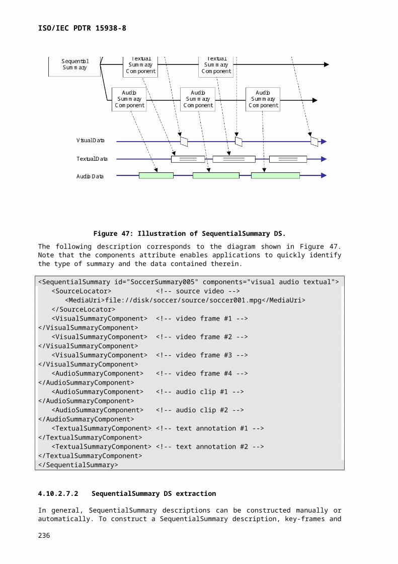
ISO/IEC PDTR 15938-8
4.11.4.3 Discrete distribution description tools
4.11.4.3.1 Discrete distribution description tools examples
The following example illustrates the use of the HistogramProbability DS for describing an eight-dimensional histogram.
<Mpeg7><DescriptionUnit xsi:type="HistogramProbabilityType"
momentNormalized="1" dim="8"><Distribution mpeg7:dim="8"> 0.125 0.0 0.0 0.25 0.125 0.25 0.25 0.0 </Distribution>
</DescriptionUnit></Mpeg7>
The following example illustrates the use of the BinomialDistribution DS for describing a one-dimensional binomial distribution.
<Mpeg7><DescriptionUnit xsi:type="BinomialDistributionType" dim="1">
<SuccessProbability mpeg7:dim="1"> 0.5 </SuccessProbability><NumOfTrials mpeg7:dim="1"> 16 </NumOfTrials>
</DescriptionUnit></Mpeg7>
The following example illustrates the use of the BinomialDistribution DS for describing a two-dimensional hypergeometric distribution.
<Mpeg7><DescriptionUnit xsi:type="HyperGeometricDistributionType" dim="2">
<NumOfSuccesses mpeg7:dim="2"> 5 5 </NumOfSuccesses><NumOfTrials mpeg7:dim="2"> 8 8 </NumOfTrials><PopulationSize mpeg7:dim="2"> 16 16 </PopulationSize>
</DescriptionUnit></Mpeg7>
The following example illustrates the use of the PoissonDistribution DS for describing a three-dimensional Poisson distribution.
<Mpeg7><DescriptionUnit xsi:type="PoissonDistributionType" dim="3">
<Lambda mpeg7:dim="3"> 0.4 0.3 0.75 </Lambda></DescriptionUnit>
</Mpeg7>
The following example illustrates the use of the GeometricDistribution DS for describing a one-dimensional geometric distribution.
<Mpeg7><DescriptionUnit xsi:type="GeometricDistributionType" dim="1">
<SuccessProbability mpeg7:dim="1"> 0.75 </SuccessProbability></DescriptionUnit>
</Mpeg7>
238

ISO/IEC PDTR 15938-8
The following example illustrates the use of the DiscreteUniformDistribution DS for describing a one-dimensional discrete uniform distribution.
<Mpeg7><DescriptionUnit xsi:type="DiscreteUniformDistributionType" dim="1">
<Range mpeg7:dim="1"> 0.125 </Range><Scale mpeg7:dim="1"> 2.0 </Scale><Shift mpeg7:dim="1"> 8.0 </Shift>
</DescriptionUnit></Mpeg7>
4.11.4.4 Continuous distribution description tools
4.11.4.4.1 Continuous distribution description tools examples
The following example illustrates the use of the GaussianDistribution DS for describing a one-dimensional Gaussian distribution.
<Mpeg7><DescriptionUnit xsi:type="GaussianDistributionType" dim="1">
<Mean mpeg7:dim="1"> 0.5 </Mean><Variance mpeg7:dim="1"> 0.25 </Variance>
</DescriptionUnit></Mpeg7>
The following example illustrates the use of the ExponentialDistribution DS for describing a two-dimensional generalized Gaussian distribution.
<Mpeg7><DescriptionUnit xsi:type="GeneralizedGaussianDistributionType" dim="2">
<Mean mpeg7:dim="2"> 0.5 0.35 </Mean><Variance mpeg7:dim="2"> 0.25 0.75 </Variance><Shape mpeg7:dim="2"> 2 2 </Shape>
</DescriptionUnit></Mpeg7>
The following example illustrates the use of the ExponentialDistribution DS for describing a two-dimensional exponential distribution.
<Mpeg7><DescriptionUnit xsi:type="ExponentialDistributionType" dim="2">
<Theta mpeg7:dim="2"> 0.5 0.25 </Theta></DescriptionUnit>
</Mpeg7>
The following example illustrates the use of the GammaDistribution DS for describing a three-dimensional Gamma distribution.
<Mpeg7><DescriptionUnit xsi:type="GammaDistributionType" dim="3">
<Theta mpeg7:dim="3"> 0.4 0.3 0.75 </Theta><Shape mpeg7:dim="3"> 8 4 16 </Shape>
</DescriptionUnit></Mpeg7>
239
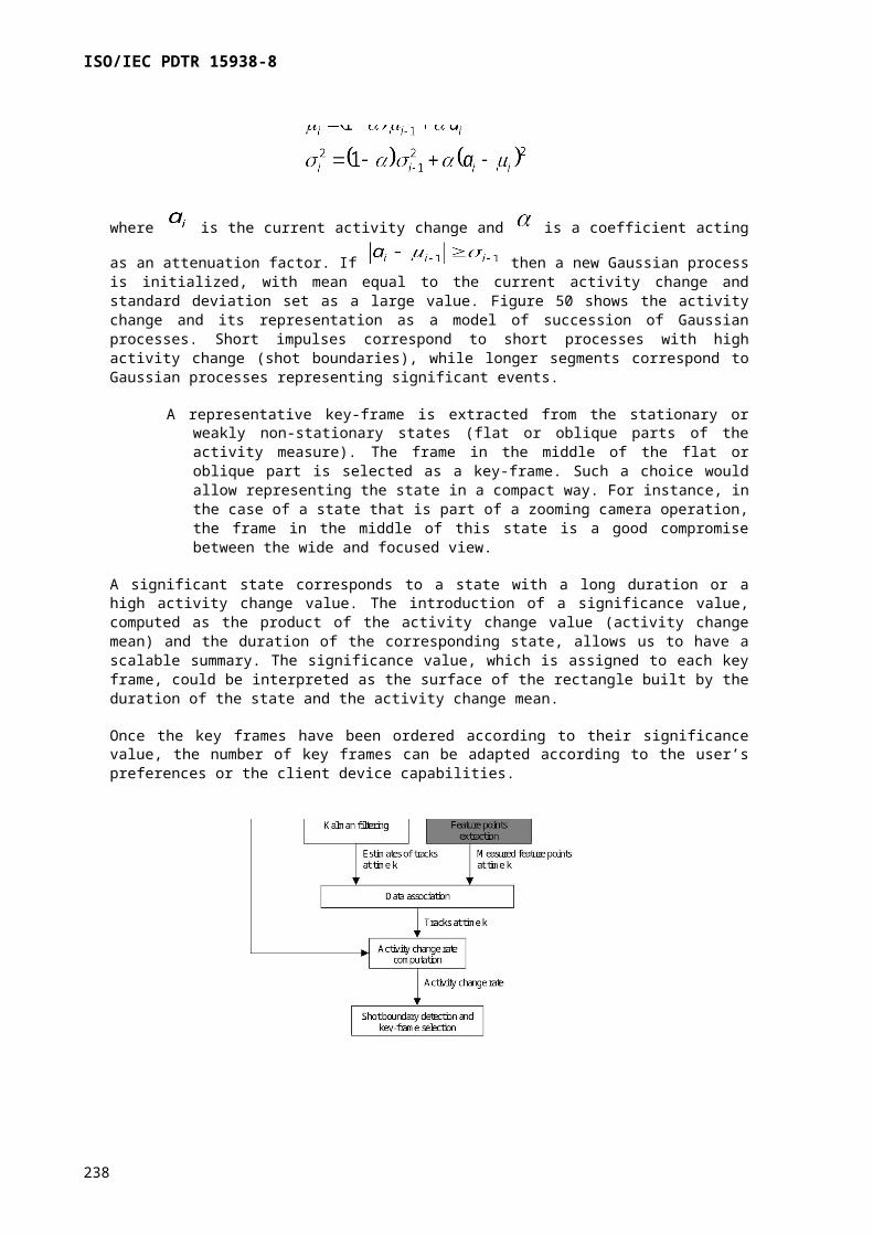
ISO/IEC PDTR 15938-8
The following example illustrates the use of the ContinuousUniformDistribution DS for describing a one-dimensional continuous uniform distribution.
<Mpeg7><DescriptionUnit xsi:type="ContinuousUniformDistributionType" dim="1">
<MaxRange mpeg7:dim="1"> 1.0 </MaxRange><MinRange mpeg7:dim="1"> 0.0 </MinRange>
</DescriptionUnit></Mpeg7>
The following example illustrates the use of the LognormalDistribution DS for describing a one-dimensional lognormal distribution.
<Mpeg7><DescriptionUnit xsi:type="LognormalDistributionType" dim="1">
<NormalMean mpeg7:dim="1"> 0.5 </NormalMean><NormalVariance mpeg7:dim="1"> 0.35 </NormalVariance>
</DescriptionUnit></Mpeg7>
4.11.4.5 Finite state model description tools
4.11.4.5.1 Finite state model description tools examples
The following example shows the use of the StateTransitionModel DS for describing a state-transition model that has three states. In this example, assume that the observed weather has one of the following states: "precipitation", "cloudy", or "sunny". Furthermore, the state-transition probabilities indicate the probability of moving from one state to another. The initial probabilities specify the initial probability of each state. The state-transition model allows questions to be answered such as, what is the probability that the weather for eight consecutive days is "sun-sun-sun-rain-rain-sun-cloudy-sun", or given that the system is in a known state, i.e., "sunny", what is the expected number of consecutive days the system will remain in that state.
<Mpeg7><Description xsi:type="ModelDescriptionType">
<Model xsi:type="StateTransitionModelType" numOfStates="3"><Initial mpeg7:dim="3"> 0.5 0.25 0.25 </Initial><Transitions mpeg7:dim="3 3"> 0.4 0.3 0.3 0.2 0.6 0.2 0.1 0.1 0.8
</Transitions><State>
<Label><Name>Precipitation </Name>
</Label></State><State>
<Label><Name>Cloudy </Name>
</Label></State><State>
<Label><Name>Sunny </Name>
</Label></State>
</Model></Description>
</Mpeg7>
240

ISO/IEC PDTR 15938-8
The following example shows the use of the StateTransitionModel DS for describing a state-transition model of the events depicted a video of a soccer game. The model describes three states: "Pass", "Shot on goal" and "Goal score". The StateTransitionModel DS describes the states, the initial state probabilities, and the transition probabilities between the states.
<Mpeg7><Description xsi:type="ModelDescriptionType">
<Model xsi:type="StateTransitionModelType" numOfStates="3"><Initial mpeg7:dim="3"> 0.25 0.5 0.25 </Initial><Transitions mpeg7:dim="3 3"> 0.2 0.2 0.6 0.1 0.8 0.1 0.3 0.3 0.4
</Transitions><State>
<Label><Name> Pass </Name>
</Label></State><State>
<Label><Name>Shot on goal </Name>
</Label></State><State>
<Label><Name>Goal score </Name>
</Label></State>
</Model></Description>
</Mpeg7>
The following example shows the use of DiscreteHiddenMarkovModelType for describing a discrete hidden markov model of events in a soccer game, such as "passes" and "goal scores".
<Mpeg7><Description xsi:type="ModelDescriptionType">
<Model xsi:type="DiscreteHiddenMarkovModelType" numOfStates="2"><Initial mpeg7:dim="2"> 0.5 0.5 </Initial><Transitions mpeg7:dim="2 2"> 0.4 0.6 0.3 0.7 </Transitions><State>
<Label><Name> Pass </Name>
</Label></State><State>
<Label><Name> Goal score </Name>
</Label></State><NumOfObservationsPerState>2</NumOfObservationsPerState><Observation> Team A pass </Observation><Observation> Team B pass </Observation><ObservationDistribution xsi:type="HistogramProbabilityType"
momentNormalized="1" dim="2"><Distribution mpeg7:dim="2"> 0.2 0.8 </Distribution>
</ObservationDistribution><NumOfObservationsPerState>2</NumOfObservationsPerState><Observation> Team A goal </Observation><Observation> Team B goal </Observation><ObservationDistribution xsi:type="HistogramProbabilityType"
momentNormalized="1" dim="2">
241

ISO/IEC PDTR 15938-8
<Distribution mpeg7:dim="2"> 0.4 0.6 </Distribution></ObservationDistribution>
</Model></Description>
</Mpeg7>
The following example shows the use of the ContinuousHiddenMarkovModel DS for describing a continuous hidden Markov model of audio sound effects. Each continuous hidden Markov model has 5 states and represents a sound effect class. The parameters of the continuous density state model can be estimated via training, for example, using the Baum-Welch algorithm. After training, the continuous HMM model consists of a 5x5 state transition matrix, a 5x1 initial state density matrix, and 5 multi-dimensional Gaussian distributions defined in terms of the mean and variance parameters. Each multi-dimensional Gaussian distribution has six dimensions corresponding to audio features comprised of 5 channels of Independent Component Analysis (ICA) data and 1 channel of spectral envelope data.
<Mpeg7><Description xsi:type="ModelDescriptionType">
<Model xsi:type="ContinuousHiddenMarkovModelType" numOfStates="5"><Initial mpeg7:dim="5"> 0.1 0.2 0.1 0.4 0.2 </Initial><Transitions mpeg7:dim="5 5">
0.2 0.2 0.6 0.0 0.0 0.1 0.2 0.1 0.3 0.3 0.4 0.2 0.1 0.1 0.20.2 0.1 0.4 0.2 0.1 0.0 0.2 0.1 0.3 0.4
</Transitions><State>
<Label><Name> State 1 </Name>
</Label></State><State>
<Label><Name> State 2 </Name>
</Label></State><State>
<Label><Name> State 3 </Name>
</Label></State><State>
<Label><Name> State 4 </Name>
</Label></State><State>
<Label><Name> State 5 </Name>
</Label></State><DescriptorModel>
<Descriptor xsi:type="BeatType"><BeatData> 1 2 3 4 5 6 </BeatData>
</Descriptor><Field xsi:type="xPathFieldType">BeatData</Field>
</DescriptorModel><ObservationDistribution xsi:type="GaussianDistributionType"
dim="6">
242

ISO/IEC PDTR 15938-8
<Mean mpeg7:dim="6"> 0.5 0.5 0.25 0.3 0.5 0.3 </Mean><Variance mpeg7:dim="6"> 0.25 0.75 0.5 0.45 0.75
0.3</Variance></ObservationDistribution><ObservationDistribution xsi:type="GaussianDistributionType"
dim="6"><Mean mpeg7:dim="6"> 0.25 0.4 0.25 0.3 0.2 0.1 </Mean><Variance mpeg7:dim="6"> 0.5 0.25 0.5 0.45 0.5 0.2</Variance>
</ObservationDistribution><ObservationDistribution xsi:type="GaussianDistributionType"
dim="6"><Mean mpeg7:dim="6"> 0.2 0.5 0.35 0.3 0.5 0.5 </Mean><Variance mpeg7:dim="6"> 0.5 0.5 0.5 0.5 0.75 0.5</Variance>
</ObservationDistribution><ObservationDistribution xsi:type="GaussianDistributionType"
dim="6"><Mean mpeg7:dim="6"> 0.5 0.3 0.25 0.2 0.5 0.6 </Mean><Variance mpeg7:dim="6"> 0.5 0.1 0.5 0.25 0.75 0.4</Variance>
</ObservationDistribution><ObservationDistribution xsi:type="GaussianDistributionType"
dim="6"><Mean mpeg7:dim="6"> 0.5 0.15 0.25 0.3 0.5 0.35 </Mean><Variance mpeg7:dim="6"> 0.5 0.75 0.5 0.5 0.75 0.35</Variance>
</ObservationDistribution></Model>
</Description></Mpeg7>
4.11.4.5.2 FiniteStateModel DS use
State-transition models can be extracted from the events along the temporal dimension of a video sequence. For example, a temporal sequence of scenes in video can be characterized by a state-transition model that describes the probabilities of transitions between scenes.
The state-transition models can be matched using the following matching metrics to determine the similarity of the underlying multimedia content being modeled:
Euclidean distance: calculates the sum of squared differences between transition probabilities.
Quadratic distance: calculates the sum of weighted quadratic distance between transition probabilities.
Weighted transition frequency: calculates the weighted sum of ratios of transition probabilities.
243
ISO/IEC PDTR 15938-8
Euclidean distance of aggregated state transitions: calculates the sum of the squared differences of aggregated transitions.
4.11.5 Analytic models
4.11.5.1.1 AnalyticModel DS examples
The example below illustrates the use of the ModelState DS to describe a an analytic model that represents a state in a finite state model. The description gives three labels for the state and gives information about the confidence and reliability of the state analytic model.
<Mpeg7><Description xsi:type="ModelDescriptionType">
<Model xsi:type="ModelStateType" confidence="0.9" reliability="0.75">
<Label relevance="0.5" confidence="0.9" reliability="0.75"><Name> Shot on goal </Name>
</Label><Label relevance="1.0" confidence="0.75" reliability="0.75">
<Name> Ball block </Name></Label><Label relevance="0.25" confidence="0.5" reliability="0.75">
<Name> Shot wide </Name></Label>
</Model></Description>
</Mpeg7>
4.11.5.2 CollectionModel DS
4.11.5.2.1 CollectionModel DS examples
The following example illustrates the use of the CollectionModel DS for describing a collection model consisting of a content collection of four images. In this example, the semantic concept is being described by the collection of images. For example, the collection of images describe the concept of "soccer shots on goal". In this example, the description gives a confidence of 0.75 and a reliability of 0.5.
<Mpeg7><Description xsi:type="ModelDescriptionType">
<Model xsi:type="CollectionModelType" confidence="0.75" reliability="0.5"
function="described"><Label>
<Name>Soccer shots on goal</Name></Label><Collection xsi:type="ContentCollectionType">
<Content xsi:type="ImageType"><Image>
244

ISO/IEC PDTR 15938-8
<MediaLocator xsi:type="ImageLocatorType"><MediaUri>soccer1.jpg</MediaUri>
</MediaLocator></Image>
</Content><Content xsi:type="ImageType">
<Image><MediaLocator xsi:type="ImageLocatorType">
<MediaUri>soccer2.jpg</MediaUri></MediaLocator>
</Image></Content><Content xsi:type="ImageType">
<Image><MediaLocator xsi:type="ImageLocatorType">
<MediaUri>soccer3.jpg</MediaUri></MediaLocator>
</Image></Content><Content xsi:type="ImageType">
<Image><MediaLocator xsi:type="ImageLocatorType">
<MediaUri>soccer4.jpg</MediaUri></MediaLocator>
</Image></Content>
</Collection></Model>
</Description></Mpeg7>
The following example illustrates the use of the CollectionModel DS for describing a model of a collection of two color descriptions. In this example, the semantic concept "Sunsets" has the function of describing the collection of descriptors.
<Mpeg7><Description xsi:type="ModelDescriptionType">
<Model xsi:type="CollectionModelType" confidence="0.75" reliability="0.5"
function="describing"><Label>
<Name> Sunsets </Name></Label><Collection xsi:type="DescriptorCollectionType">
<Descriptor xsi:type="ScalableColorType" numOfCoeff="16" numOfBitplanesDiscarded="0"><Coeff> 1 2 3 4 5 6 7 8 9 0 1 2 3 4 5 6 </Coeff>
</Descriptor><Descriptor xsi:type="ScalableColorType" numOfCoeff="16"
numOfBitplanesDiscarded="0"><Coeff> 1 2 3 4 5 6 7 8 9 0 1 2 3 4 5 6 </Coeff>
</Descriptor></Collection>
</Model></Description>
</Mpeg7>
The following example illustrates the use of the CollectionModel DS for describing a collection of of four concepts. The concept collection has a semantic label: "soccer stadium objects", that is, the
245

ISO/IEC PDTR 15938-8
semantic concept has the function of describing the collection of concepts. In this example, the confidence is 0.75 and reliability is 0.5.
<Mpeg7><Description xsi:type="ModelDescriptionType">
<Model xsi:type="CollectionModelType" confidence="0.75" reliability="0.5"
function="describing"><Label>
<Name>Soccer stadium objects</Name></Label><Collection xsi:type="ConceptCollectionType">
<Concept xsi:type="ObjectType"><Label>
<Name> Ball </Name></Label>
</Concept><Concept xsi:type="ObjectType">
<Label><Name> Goal </Name>
</Label></Concept><Concept xsi:type="ObjectType">
<Label><Name> Seats </Name>
</Label></Concept><Concept xsi:type="ObjectType">
<Label><Name> Water </Name>
</Label></Concept>
</Collection></Model>
</Description></Mpeg7>
4.11.5.3 DescriptorModel DS
4.11.5.3.1 DescriptorModel DS examples
The following example illustrates the use of the DescriptorModel DS for describing a descriptor model of the ScalableColor descriptor. The DescriptorModel DS specifies that the descriptor model is formed from the Coefficients element of the ScalableColor D (defined in ISO/IEC 15938-3). For example, in the DescriptorModel for ScalableColorType, the value of numOfCoefficients="16" is constant in the descriptor model.
<mpeg7><Description xsi:type="ModelDescriptionType">
<Model xsi:type="DescriptorModelType"><Descriptor xsi:type="ScalableColorType" numOfCoeff="16"
numOfBitplanesDiscarded="0"><Coeff> 1 2 3 4 5 6 7 8 9 0 1 2 3 4 5 6 </Coeff>
</Descriptor><Field>Coeff</Field>
</Model></Description>
</Mpeg7>
246

ISO/IEC PDTR 15938-8
The following example illustrates the use of the DescriptorModel DS for describing a descriptor model of the ContourShape descriptor. The DescriptorModel DS specifies that the descriptor model is formed from the concatenation of six elements of the ContourShape D (defined in ISO/IEC 15938-3). All other elements and attributes not mentioned in the field statements are assumed to be constant in the descriptor models, taking the values specified in the example Descriptors.
<Mpeg7><Description xsi:type="ModelDescriptionType">
<Model xsi:type="DescriptorModelType"><Descriptor xsi:type="ContourShapeType">
<GlobalCurvature> 3 5 </GlobalCurvature><PrototypeCurvature> 4 7 </PrototypeCurvature><HighestPeakY>2</HighestPeakY><Peak peakX="4" peakY="2"/><Peak peakX="3" peakY="5"/><Peak peakX="7" peakY="1"/>
</Descriptor><Field>GlobalCurvature</Field><Field>PrototypeCurvature</Field><Field>HighestPeakY</Field><Field>Peak</Field>
</Model></Description>
</Mpeg7>
4.11.5.4 ProbabilityModelClass DS
4.11.5.4.1 ProbabilityModelClass DS examples
The following example illustrates the use of the ProbabilityModelClass DS for describing a probability model class that characterizes a class of "Nature scene" images by representing the statistics associated with the color features of the images of that class. For example, the specification below indicates that the Coefficients element of the ScalableColor D (defined in ISO/IEC 15938-3) for the Nature scene images has a centroid or mean value of (0.5, 0.5, …) and a variance of (0.25, 0.75, …).
<mpeg7><Description xsi:type="ModelDescriptionType">
<Model xsi:type="ProbabilityModelClassType" confidence="0.75" reliability="0.5"><Label>
<Name>Nature scenes</Name></Label><DescriptorModel>
<Descriptor xsi:type="ScalableColorType" numOfCoeff="16" numOfBitplanesDiscarded="0"><Coeff> 1 2 3 4 5 6 7 8 9 0 1 2 3 4 5 6 </Coeff>
</Descriptor><Field>Coeff</Field>
</DescriptorModel><ProbabilityModel xsi:type="ProbabilityDistributionType"
confidence="1.0" dim="16"><Mean mpeg7:dim="16"> 0 1 2 3 4 5 6 7 8 9 0 1 2 3 4 5 </Mean><Variance mpeg7:dim="16"> 2 3 4 5 6 7 8 9 0 1 2 3 4 5 6 5
</Variance></ProbabilityModel>
</Model>
247

ISO/IEC PDTR 15938-8
</Description></Mpeg7>
The following example illustrates the use of the ProbabilityModelClass DS for describing a probability model that characterizes checker patterns using a probability model of EdgeHistogram D (see ISO/IEC 15938-3).
<Mpeg7><Description xsi:type="ModelDescriptionType">
<Model xsi:type="ProbabilityModelClassType" confidence="0.75" reliability="0.5"><Label relevance="0.75">
<Name>Checker patterns</Name></Label><DescriptorModel>
<Descriptor xsi:type="EdgeHistogramType"><BinCounts> 3 5 2 5 . . . 6 </BinCounts>
</Descriptor><Field>BinCounts</Field>
</DescriptorModel><ProbabilityModel xsi:type="ProbabilityDistributionType"
confidence="0.75" dim="80"><Mean mpeg7:dim="80"> 5 3 9 4 . . . 5 </Mean><Variance mpeg7:dim="80"> 4.5 5.0 8.0 7.5 . . . 5.2
</Variance></ProbabilityModel>
</Model></Description>
</Mpeg7>
The following example illustrates the use of the ProbabilityModelClass DS for describing a probability model that characterizes oval shapes using a probability model of RegionShape D (see ISO/IEC 15938-3).
<Mpeg7><Description xsi:type="ModelDescriptionType">
<Model xsi:type="ProbabilityModelClassType" confidence="0.75" reliability="0.5"><Label relevance="0.75">
<Name> Ovals </Name></Label><DescriptorModel>
<Descriptor xsi:type="RegionShapeType"><MagnitudeOfART> 3 5 2 5 . . . 6 </MagnitudeOfART>
</Descriptor><Field>MagnitudeOfART</Field>
</DescriptorModel><ProbabilityModel xsi:type="ProbabilityDistributionType"
confidence="1.0" dim="35"><Mean dim="35"> 4 8 6 9 . . . 5 </Mean><Variance dim="35"> 1.3 2.5 5.0 4.5 . . . 3.2 </Variance>
</ProbabilityModel></Model>
</Description></Mpeg7>
248

ISO/IEC PDTR 15938-8
The following example illustrates the use of the ProbabilityModelClass DS for describing a probability model that characterizes silhouettes using a probability model of ContourShape D (see ISO/IEC 15938-3).
<Mpeg7><Description xsi:type="ModelDescriptionType">
<Model xsi:type="ProbabilityModelClassType" confidence="0.75" reliability="0.5"><Label relevance="0.75">
<Name> Silhouettes </Name></Label><DescriptorModel>
<Descriptor xsi:type="ContourShapeType"><GlobalCurvature> 3 5 </GlobalCurvature><PrototypeCurvature> 4 7 </PrototypeCurvature><HighestPeakY>2</HighestPeakY><Peak peakX="4" peakY="2"/><Peak peakX="3" peakY="5"/><Peak peakX="7" peakY="1"/>
</Descriptor><Field>GlobalCurvature</Field><Field>PrototypeCurvature</Field><Field>HighestPeakY</Field><Field>Peak</Field>
</DescriptorModel><ProbabilityModel xsi:type="ProbabilityDistributionType"
confidence="1.0" dim="11"><Mean mpeg7:dim="11"> 3 9 7 4 6 9 1 2 6 8 9</Mean><Variance mpeg7:dim="11"> 3.4 5.4 9.1 1.8 2.3 6.5 7.9 1.2 3.4
3.3 1.0 </Variance>
</ProbabilityModel></Model>
</Description></Mpeg7>
4.11.6 Cluster models
4.11.6.1.1 ClusterModel DS examples
The following example illustrates the use of the ClusterModel DS for describing a cluster model consisting of a set of examples of two scalable color descriptions. The cluster models have a semantic label: "Nature scenes". The example describes also the probability model of the ScalableColor D (see ISO/IEC 15938-3).
<Mpeg7><Description xsi:type="ModelDescriptionType">
<Model xsi:type="ClusterModelType" confidence="0.75" reliability="0.5">
<Label><Name> Nature scenes </Name>
</Label><Collection xsi:type="DescriptorCollectionType">
<Descriptor xsi:type="ScalableColorType" numOfCoeff="16" numOfBitplanesDiscarded="0"><Coeff> 1 2 3 4 5 6 7 8 9 0 1 2 3 4 5 6 </Coeff>
</Descriptor><Descriptor xsi:type="ScalableColorType" numOfCoeff="16"
249

ISO/IEC PDTR 15938-8
numOfBitplanesDiscarded="0"><Coeff> 1 2 3 4 5 6 7 8 9 0 1 2 3 4 5 6 </Coeff>
</Descriptor></Collection><DescriptorModel>
<Descriptor xsi:type="ScalableColorType" numOfCoeff="16" numOfBitplanesDiscarded="0"><Coeff> 1 2 3 4 5 6 7 8 9 0 1 2 3 4 5 6 </Coeff>
</Descriptor><Field>Coeff</Field>
</DescriptorModel><ProbabilityModel xsi:type="ProbabilityDistributionType"
confidence="1.0" dim="16"><Mean mpeg7:dim="16"> 0 1 2 3 4 5 6 7 8 9 0 1 2 3 4 5 </Mean><Variance mpeg7:dim="16"> 2 3 4 5 6 7 8 9 0 1 2 3 4 5 6 5
</Variance></ProbabilityModel>
</Model></Description>
</Mpeg7>
4.11.7 Classification models
Information on extraction and use is not provided.
4.11.7.1 ClusterClassificationModel DS
4.11.7.1.1 ClusterClassificationModel examples
The following example illustrates the use of the ClusterClassificationModel DS for describing a cluster classification model related to scenes from a soccer game. In this example, the ClusterClassificationModel is comprised of two ClusterModels. The first ClusterModel describes a cluster of two images that form the class with label "Soccer shots on goal". The second ClusterModel describes a cluster of two images that form the class with label "Goal scores".
<Mpeg7><Description xsi:type="ModelDescriptionType">
<Model xsi:type="ClusterClassificationModelType" confidence="0.9" reliability="0.8" complete="true" redundant="false"><ClusterModel confidence="0.75" reliability="0.5">
<Label><Name> Soccer shots on goal </Name>
</Label><Collection xsi:type="ContentCollectionType">
<Content xsi:type="ImageType"><Image>
<MediaLocator xsi:type="ImageLocatorType"><MediaUri>soccer1.jpg</MediaUri>
</MediaLocator></Image>
</Content><Content xsi:type="ImageType">
<Image><MediaLocator xsi:type="ImageLocatorType">
<MediaUri>soccer2.jpg</MediaUri></MediaLocator>
</Image></Content>
250
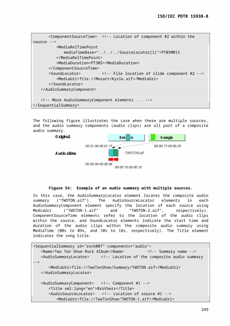
ISO/IEC PDTR 15938-8
</Collection></ClusterModel><ClusterModel confidence="0.9" reliability="0.75">
<Label><Name> Goal scores </Name>
</Label><Collection xsi:type="ContentCollectionType">
<Content xsi:type="ImageType"><Image>
<MediaLocator xsi:type="ImageLocatorType"><MediaUri>soccer3.jpg</MediaUri>
</MediaLocator></Image>
</Content><Content xsi:type="ImageType">
<Image><MediaLocator xsi:type="ImageLocatorType">
<MediaUri>soccer4.jpg</MediaUri></MediaLocator>
</Image></Content>
</Collection></ClusterModel>
</Model></Description>
</Mpeg7>
The following example illustrates the use of the ClusterClassificationModel DS for describing a cluster classification model related to images depicting nature scenes. The ClusterClassificationModel is comprised of two ClusterModels. The first ClusterModel describes a collection of two scalable color descriptions that forms the class with label "Sunsets". The second ClusterModel describes a collection of two scalable color descriptions that forms the class with label "Nature scenes".
<Mpeg7><Description xsi:type="ModelDescriptionType">
<Model xsi:type="ClusterClassificationModelType" confidence="0.95" reliability="0.75" complete="true" redundant="false"><ClusterModel confidence="0.8" reliability="0.75">
<Label relevance="0.75"><Name>Sunsets</Name>
</Label><Collection xsi:type="DescriptorCollectionType">
<Descriptor xsi:type="ScalableColorType" numOfCoeff="16" numOfBitplanesDiscarded="0"><Coeff> 1 2 3 4 5 6 7 8 9 0 1 2 3 4 5 6 </Coeff>
</Descriptor><Descriptor xsi:type="ScalableColorType" numOfCoeff="16"
numOfBitplanesDiscarded="0"><Coeff> 1 2 3 4 5 6 7 8 9 0 1 2 3 4 5 6 </Coeff>
</Descriptor></Collection>
</ClusterModel><ClusterModel confidence="0.75" reliability="0.5">
<Label><Name>Nature scenes</Name>
</Label><Collection xsi:type="DescriptorCollectionType">
<Descriptor xsi:type="ScalableColorType" numOfCoeff="16" numOfBitplanesDiscarded="0">
251

ISO/IEC PDTR 15938-8
<Coeff> 1 2 3 4 5 6 7 8 9 0 1 2 3 4 5 6 </Coeff></Descriptor><Descriptor xsi:type="ScalableColorType" numOfCoeff="16"
numOfBitplanesDiscarded="0"><Coeff> 1 2 3 4 5 6 7 8 9 0 1 2 3 4 5 6 </Coeff>
</Descriptor></Collection>
</ClusterModel></Model>
</Description></Mpeg7>
4.11.7.2 ProbabilityClassificationModel DS
4.11.7.2.1 ProbabilityClassificationModel DS examples
The following example illustrates the use of the ProbabilityClassificationModel DS for describing a probability classification model for sunset and nature images. The ProbabilityClassificationModel DS is comprised of two instances of ProbabilityModelClass DS. The first ProbabilityModelClass DS instance specifies a class of scalable color descriptors that forms with label "Sunsets". The second ProbabilityModelClass DS instance specifies a class scalable color descriptors with label "Nature scenes".
<Mpeg7><Description xsi:type="ModelDescriptionType">
<Model xsi:type="ProbabilityClassificationModelType" confidence="0.95"
reliability="0.75" complete="true" redundant="false"><ProbabilityModelClass confidence="0.9" reliability="0.5">
<Label><Name>Sunsets</Name>
</Label><DescriptorModel>
<Descriptor xsi:type="ScalableColorType" numOfCoeff="16" numOfBitplanesDiscarded="0"><Coeff> 4 5 6 7 8 9 0 1 2 3 4 5 6 1 2 3</Coeff>
</Descriptor><Field>Coeff</Field>
</DescriptorModel><ProbabilityModel xsi:type="ProbabilityDistributionType"
confidence="1.0" dim="16"><Mean mpeg7:dim="16"> 0 1 2 3 4 5 6 7 8 9 0 1 2 3 4 5
</Mean><Variance mpeg7:dim="16"> 5 6 7 8 9 0 1 2 3 4 5 6 5 2 3 4 </Variance>
</ProbabilityModel></ProbabilityModelClass><ProbabilityModelClass confidence="0.9" reliability="0.8">
<Label><Name>Nature scenes</Name>
</Label><DescriptorModel>
<Descriptor xsi:type="ScalableColorType" numOfCoeff="16" numOfBitplanesDiscarded="0"><Coeff> 1 2 3 4 5 6 7 8 9 0 1 2 3 4 5 6 </Coeff>
</Descriptor><Field>Coeff</Field>
</DescriptorModel><ProbabilityModel xsi:type="ProbabilityDistributionType"
252

ISO/IEC PDTR 15938-8
confidence="1.0" dim="16"><Mean mpeg7:dim="16"> 3 4 5 0 1 2 3 4 5 6 7 8 9 0 1 2
</Mean><Variance mpeg7:dim="16"> 5 6 5 2 3 4 5 6 7 8 9 0 1 2 3 4 </Variance>
</ProbabilityModel></ProbabilityModelClass>
</Model></Description>
</Mpeg7>
253
ISO/IEC PDTR 15938-8
4.12 User interaction tools
4.12.1 Introduction
Clause 4.12 specifies the following description tools related to user interaction with multimedia content.
Table 13: Overview of User Interaction Tools.Tool Functionality
User Preferences Tools for describing user preferences pertaining to multimedia content, enabling effective user interaction and personalization of content access and consumption. See clause 4.12.2.
Usage History Tools for describing usage history of users of multimedia content, enabling effective user interaction and personalization of content access and consumption. See clause 4.12.3.
4.12.2 User preferences
4.12.2.1 Basic user preference tools
4.12.2.1.1 Basic user preference tools examples
The PreferenceCondition D is used to describe a time or place or a time and place combination that can be associated with a particular set of browsing, filtering and search preferences. For example, a user may have preferences for different broadcast sports programs during different seasons of the year. Similarly, a user may have preference for programs in English language when the user is traveling in Japan. The following example highlights the case where the user’s stated genre preferences apply every day during primetime hours (8PM to 11PM).
<UserPreferences><FilteringAndSearchPreferences>
<ClassificationPreferences><Genre href="urn:mpeg:mpeg7:cs:GenreCS:2001:2.1.2">
<Name>Comedy</Name></Genre>
</ClassificationPreferences><PreferenceCondition>
<Time recurrence="daily"><TimePoint>T20:00+01:00</TimePoint><Duration>PT3H</Duration>
</Time></PreferenceCondition>
</FilteringAndSearchPreferences></UserPreferences>
In the next example, the preferences of a user who is interested in a yearly recurring basketball tournament (lasting one week) can be given by the following PreferenceCondition instance.
<UserPreferences><FilteringAndSearchPreferences>
<ClassificationPreferences><Genre href="urn:mpeg:mpeg7:cs:GenreCS:2001:1.6.9">
<Name>Basketball</Name>
254

ISO/IEC PDTR 15938-8
</Genre></ClassificationPreferences><PreferenceCondition>
<Time recurrence="annually" numOfRecurrences="5"><TimePoint>2001-03-28T8:00</TimePoint><Duration>P7D</Duration>
</Time></PreferenceCondition>
</FilteringAndSearchPreferences></UserPreferences>
4.12.2.2 UserPreferences DS
4.12.2.2.1 UserPreferences DS examples
The UserPreferences DS is used to specify user's preferences pertaining to filtering, searching and browsing of multimedia content and can be used for personalized viewing and listening. Filtering and search preferences describe, for example, favorite titles, genres, actors and sources of content. This information can be used to find preferred multimedia content by matching it with information in multimedia content descriptions. Browsing preferences, for example, describe preferred views of favorite content, where preferences may be dependent on usage conditions such as available bandwidth or the time the user has to consume the information. This allows the user to navigate and access different views of the content in a personalized manner. An example UserPreferences description is as follows. Subelements of the FilteringAndSearchPreferences and BrowsingPreferences are introduced in later subclauses. Note that XML comments are used to replace description details.
<UserPreferences allowAutomaticUpdate="true"><UserIdentifier>
<!-- User preferences identification elements --></UserIdentifier><FilteringAndSearchPreferences>
<!-- Filtering and search preference elements --></FilteringAndSearchPreferences><BrowsingPreferences>
<!-- Browsing preference elements --></BrowsingPreferences>
</UserPreferences>
4.12.2.2.2 UserPreferences DS extraction
In general, UserPreferences descriptions can be constructed manually or automatically. A UserPreferences description may be entered manually by the multimedia content user. Alternatively, a UserPreferences description may be constructed automatically based on the user's content usage history.
4.12.2.2.3 UserPreferences DS use
In general, the descriptions of the user's preferences can be used to automatically find preferred multimedia content and to present preferred views of the content to the user.
In the following, a method is described for automatic filtering of multimedia content using content descriptions and user preference descriptions. Each individual component of the FilteringAndSearchPreferences DS in the UserPreferences DS corresponds to a test or matching operation against components of descriptions of multimedia content. Examples of individual components are the Role, GivenName, FamilyName, DatePeriod elements and the Genre elements in the partial user preference description shown below.
255

ISO/IEC PDTR 15938-8
<UserPreferences><UsagePreferences>
<FilteringAndSearchPreferences><CreationPreferences>
<Creator><Role><Name>Actor</Name></Role><Agent xsi:type="PersonType">
<Name><GivenName>Harrison</GivenName><FamilyName>Ford</FamilyName>
</Name></Agent>
</Creator><DatePeriod>
<TimePoint>1995-01-01</TimePoint><Duration>P1825D</Duration>
</DatePeriod></CreationPreferences><ClassificationPreferences>
<Genre><Name>News</Name></Genre><Genre><Name>Sports</Name></Genre><Genre><Name>Documentary</Name></Genre>
</ClassificationPreferences></FilteringAndSearchPreferences>
</UsagePreferences></UserPreferences>
For example, the name values of each Genre element in this user preference description can be matched against the name values of the Genre element in the following partial content description. Likewise, the date values of the DatePeriod element can be matched against the date value of the Release element of the content description below.
<MultiMediaContent><AudioVisual>
<CreationInformation><Creation>
<Title xml:lang="en">Afternoon news</Title></Creation><Classification>
<Genre><Name xml:lang="en">News</Name></Genre><Release date="1998-06-16T21:30+01:00">
<Country>es</Country></Release>
</Classification></CreationInformation>
</AudioVisual></MultiMediaContent>
The method for testing individual components is may involve (sub)string matching, boolean value matching, numerical value range tests, counting and other operations. Furthermore, each test may result in an exact or a partial match. For example, textual Genre name values are tested using case-insensitive string matching. Matching date values, on the other hand, requires numerical comparison operations.
After individual preference components are tested, the results of these tests must be combined into a single test result that reflects the user’s overall preferences. The individual test results can be combined according to the hierarchy of the UserPreferences description. Each parent test becomes a combination of its children tests, and this continues up the hierarchy, yielding one composite test result. The combination of children tests within a single parent may depend on the types of the
256

ISO/IEC PDTR 15938-8
elements being tested. For example, the partial user preferences description above specifies a preference for content with an actor having first name "Harrison" and having last name "Ford". Therefore, in this case, an intersection operator can be used to combine the individual test results. As another example, the user preferences description above specifies preferences for multiple genres: "News", "Sports" and "Documentaries". Different multimedia programs, each with a different genre, may each satisfy the individual tests against these genre preferences. Therefore, in this case, a union operator can be used to combine the individual test results.
The combination of the user's preferences and the overall matching result against multimedia content descriptions can be used to rank-order the corresponding multimedia content items and/or to automatically filter the content items.
4.12.2.3 UserIdentifier datatype
4.12.2.3.1 UserIdentifier datatype examples
The UserIdentifier datatype may be used to identify a particular user preference description and distinguish it from other user preference descriptions. The Name element may contain the user's actual name, a nickname, a user's account name or email address, or any other name. The same user may have multiple user preference descriptions, each identified by a different value of Name, for use under different usage conditions. Also, a group of persons can use a single set of user preferences, using a single identifier for the group. The following example illustrates a description owned by user "Jane", who desires to keep the identifier part of this description private.
<UserPreferences><UserIdentifier protected="true">
<Name xml:lang="en">Jane</Name></UserIdentifier><FilteringAndSearchPreferences protected="true">
<!-- Filtering and search preference elements --></FilteringAndSearchPreferences><BrowsingPreferences protected="true">
<!-- Browsing preference elements --></BrowsingPreferences>
</UserPreferences>
4.12.2.4 FilteringAndSearchPreferences DS
4.12.2.4.1 FilteringAndSearchPreferences DS examples
In general, the FilteringAndSearchPreferences DS may be used to search or filter multimedia content by matching the values of components of the filtering and search preferences to the values of parts of descriptions of multimedia content. For instance, the values of CreationPreferences may be matched to instances of the Creation DS as defined in subclause 9.1.2. The values of ClassificationPreferences may be matched to instances of the Classification DS as defined in subclause 9.1.3. The values of SourcePreferences may be matched to instances of the MediaInformation DS, CreationInformation DS or UsageInformation DS as defined in clauses 8, 9 and 10.
Each individual component of the FilteringAndSearchPreferences DS corresponds to a test or matching operation by a content filtering or search application against components of descriptions of multimedia content. The FilteringAndSearchPreferences DS by itself does not imply any specific normative behavior of such an application regarding the combination of individual preference components. The most basic behavior of an application would be consistent with viewing the structure of the FilteringAndSearchPreferences DS as a simple aggregation of individual preference components. However, the structure of the DS strongly suggests restrictions on the behavior expected from such an application by the user, with regard to combinations of preference components. A few examples are discussed in the following.
257

ISO/IEC PDTR 15938-8
For example, when multiple sibling elements of the same type are present in a user preference description, such as the multiple Genre elements in the following description, an application may tend to favor multimedia content matching the first Genre ("Daily news") or the second Genre ("Sports"). Note that the exact behavior may also be made to depend on whether the particular element in the user preference description can be present only once in the content description or not.
<FilteringAndSearchPreferences><ClassificationPreferences>
<Genre href="urn:mpeg:mpeg7:cs:GenreCS:2001:1.3.1"><Name>Daily news</Name>
</Genre><Genre href="urn:mpeg:mpeg7:cs:GenreCS:2001:1.6">
<Name>Sports</Name></Genre>
</ClassificationPreferences></FilteringAndSearchPreferences>
As another example, in the presence of a negative preferenceValue, such as for one Genre element among multiple sibling Genre preference elements, an application may tend to suppress multimedia content matching the first Genre ("Daily news") and favor multimedia content that matches the Genre with a positive preferenceValue ("Sports").
<FilteringAndSearchPreferences><ClassificationPreferences>
<Genre preferenceValue="-10" href="urn:mpeg:mpeg7:cs:GenreCS:2001:1.3.1">
<Name>Daily news</Name></Genre><Genre preferenceValue="10"
href="urn:mpeg:mpeg7:cs:GenreCS:2001:1.6"><Name>Sports</Name>
</Genre></ClassificationPreferences>
</FilteringAndSearchPreferences>
Furthermore, when multiple sibling elements of different types are present in a description, such as the Genre and Language elements in the following description, an application may tend to favor multimedia content matching the Genre ("Daily news") and with the correct Language ("en") over content that satisfies only one (or none) of the tests.
<FilteringAndSearchPreferences><ClassificationPreferences>
<Language>en</Language><Genre href="urn:mpeg:mpeg7:cs:GenreCS:2001:1.3.1">
<Name>Daily news </Name></Genre>
</ClassificationPreferences></FilteringAndSearchPreferences>
The following is an example using the hierarchical structure of the FilteringAndSearchPreferences DS and using multiple preferenceValue attributes. The preferenceValue attributes express the weight of a user preference component (and its content) relative to other components. This example contains three sibling FilteringAndSearchPreferences elements, each of which contains preferences on the genre of multimedia content, indicating that the user prefers content of genre "news" over content of genre "documentary" or "sports". However, within the "news" genre, the user has a preference for a particular presenter over another presenter, as indicated by the child
258

ISO/IEC PDTR 15938-8
FilteringAndSearchPreferences element and the preferenceValue attributes of sibling Creator elements. And within the "sports" genre, the user has a higher preference for "soccer" than for "baseball", as indicated by the child FilteringAndSearchPreferences element and the preferenceValue attributes of sibling Genre elements.
An application may attempt to match this example description against a description of multimedia content by using a bottom-up procedure. That is, the application may attempt to match the leaf Creator and leaf Genre elements first, resulting in individual matching scores. Then, matching scores among sibling children components may be weighed by the preference values, combined, and propagated to their parent component (in this case, CreationPreferences or ClassificationPreferences components). This procedure can be repeated across the hierarchy, finally resulting in a composite matching score for a content description.
<FilteringAndSearchPreferences preferenceValue="90"><SourcePreferences>
<DisseminationSource>KBS1</DisseminationSource></SourcePreferences><FilteringAndSearchPreferences preferenceValue="80">
<ClassificationPreferences><Genre href="urn:mpeg:mpeg7:cs:GenreCS:2001:1.3.1">
<Name>Daily news</Name></Genre>
</ClassificationPreferences><FilteringAndSearchPreferences>
<CreationPreferences><Creator preferenceValue="70">
<Role href="urn:mpeg:mpeg7:cs:RoleCS:2001:ANCHOR"/><Agent xsi:type="PersonType">
<Name><GivenName>Tom Brokite</GivenName></Name></Agent>
</Creator><Creator preferenceValue="90">
<Role href="urn:mpeg:mpeg7:cs:RoleCS:2001:ANCHOR"/><Agent xsi:type="PersonType">
<Name><GivenName>Jerry Pack</GivenName></Name></Agent>
</Creator></CreationPreferences>
</FilteringAndSearchPreferences></FilteringAndSearchPreferences><FilteringAndSearchPreferences preferenceValue="70">
<ClassificationPreferences><Genre href="urn:mpeg:mpeg7:cs:GenreCS:2001:1.13">
<Name>Documentary</Name></Genre>
</ClassificationPreferences></FilteringAndSearchPreferences><FilteringAndSearchPreferences preferenceValue="60">
<ClassificationPreferences><Genre href="urn:mpeg:mpeg7:cs:GenreCS:2001:1.6">
<Name>Sports</Name></Genre>
</ClassificationPreferences><FilteringAndSearchPreferences>
<ClassificationPreferences><Genre preferenceValue="60"
href="urn:mpeg:mpeg7:cs:GenreCS:2001:1.6.65"><Name>Soccer</Name>
</Genre><Genre preferenceValue="50"
href="urn:mpeg:mpeg7:cs:GenreCS:2001:1.6.8">
259

ISO/IEC PDTR 15938-8
<Name>Baseball</Name></Genre>
</ClassificationPreferences></FilteringAndSearchPreferences>
</FilteringAndSearchPreferences></FilteringAndSearchPreferences>
It should be noted that the specific method for testing individual components is not normative and may involve (sub)string matching, numerical comparisons, counting and other operations. Here, it is the syntax and semantics of the individual components that strongly suggest restrictions on the set of useful test operators to be used by a search or filtering application. For example, if the Genre name is represented in textual form, an application may use some form of case-insensitive string matching of the user preference element against the value of the appropriate element of a program description. Matching date values, on the other hand, may require numerical comparison operations.
Note further that a filtering or search application may test a single component of the UserPreferences DS against one or more components of the content description. For example, a Title element of the CreationPreferences DS may naturally be tested against the Title value of the content description. On the other hand, a key phrase specified with the Keyword element in the same DS may be matched with multiple textual components of content descriptions, such as the title, abstract or others. The specific matching methodology is non-normative and depends on the user's search or filtering application; however, not all choices make sense.
4.12.2.5 CreationPreferences DS
4.12.2.5.1 CreationPreferences DS examples
In the following example, the user is expressing preference for content that is created between the years 1995 and 2000 (1825 days) and describes preferred actors or actresses, each with a relative preferenceValue attribute.
<UserPreferences><FilteringAndSearchPreferences>
<CreationPreferences><Creator preferenceValue="18">
<Role href="urn:mpeg:mpeg7:cs:RoleCS:2001:ACTOR"/><Agent xsi:type="PersonType">
<Name><GivenName>Meg</GivenName><FamilyName>Ryan</FamilyName>
</Name></Agent>
</Creator><Creator preferenceValue="19">
<Role href="urn:mpeg:mpeg7:cs:RoleCS:2001:ACTOR"/><Agent xsi:type="PersonType">
<Name><GivenName>Cameron</GivenName><FamilyName>Diaz</FamilyName>
</Name></Agent>
</Creator><Creator preferenceValue="20">
<Role href="urn:mpeg:mpeg7:cs:RoleCS:2001:ACTOR"/><Agent xsi:type="PersonType">
<Name><GivenName>Harrison</GivenName><FamilyName>Ford</FamilyName>
</Name>
260

ISO/IEC PDTR 15938-8
</Agent></Creator><DatePeriod>
<TimePoint>1995-01-01</TimePoint><Duration>P1825D</Duration>
</DatePeriod></CreationPreferences>
</FilteringAndSearchPreferences></UserPreferences>
4.12.2.6 ClassificationPreferences DS
4.12.2.6.1 ClassificationPreferences DS examples
The ClassificationPreferences DS can be used to specify the user's preferred language or a favorite genre (e.g., "science-fiction movies", "business news" or "pop-music") or preferred country of origin (e.g. music from France). In the following example, the user prefers news programs with closed captions in English, when he/she is in Japan. In this example, the user also prefers movies that are spoken in English and have been reviewed by Roger Ebert and rated at 10 (where 10 is the best rating) and have a PG-13 parental rating label according to the MPAA (Motion Picture Association of America) rating scheme. Multiple instantiations of ClassificationPreferences can be ranked by the application according to the values of their individual preferenceValue attributes.
<UserPreferences allowAutomaticUpdate="false"><FilteringAndSearchPreferences>
<ClassificationPreferences preferenceValue="10"><LanguageFormat>closedCaptions</LanguageFormat><CaptionLanguage>en</CaptionLanguage><Genre href="urn:mpeg:mpeg7:cs:GenreCS:2001:1.3.1">
<Name>Daily news</Name></Genre>
</ClassificationPreferences><ClassificationPreferences preferenceValue="12">
<Language>en</Language><Genre href="urn:mpeg:mpeg7:cs:GenreCS:2001:8">
<Name>Movies</Name></Genre><Review>
<Rating><RatingValue>10</RatingValue> <RatingScheme best="10" worst="1" style="higherBetter"/>
</Rating><Reviewer xsi:type="PersonType">
<Name><FamilyName>Ebert</FamilyName><GivenName>Roger</GivenName>
</Name></Reviewer>
</Review><ParentalGuidance>
<ParentalRating href="urn:mpeg:mpeg7:cs:MPAAParentalRatingCS:2001:PG-13"><Name>PG-13</Name>
</ParentalRating><Region>us</Region>
</ParentalGuidance></ClassificationPreferences><PreferenceCondition>
<Place>
261

ISO/IEC PDTR 15938-8
<Name xml:lang="en">Japan</Name><Region>jp</Region>
</Place></PreferenceCondition>
</FilteringAndSearchPreferences></UserPreferences>
4.12.2.7 SourcePreferences DS
4.12.2.7.1 SourcePreferences DS examples
The SourcePreferences DS can be used to specify preference for sources of the content, e.g. terrestrial versus satellite. If the user has access to broadcast only, the user may not be interested in program offerings from the satellite channels. In the following example, the user has a preference for "Star Trek" programs, and content that is available from terrestrial broadcast on the day of May 23, 2000. The user has a particular preference for programs from BBC 1 and prefers content provided by the BBC in general. Such a description is useful in creating personalized electronic program guides.
<UserPreferences><FilteringAndSearchPreferences>
<CreationPreferences><Title xml:lang="en" type="original">Star Trek</Title>
</CreationPreferences><SourcePreferences>
<DisseminationFormat href="urn:mpeg:mpeg7:cs:DisseminationFormatCS:2001:1">
<Name>Terrestrial</Name></DisseminationFormat><DisseminationSource>BBC 1</DisseminationSource><DisseminationDate>
<TimePoint>2000-05-23</TimePoint></DisseminationDate><Disseminator>
<Role href="urn:mpeg:mpeg7:cs:RoleCS:2001:PUBLISHER"/><Agent xsi:type="OrganizationType><Name>BBC</Name></Agent>
</Disseminator></SourcePreferences>
</FilteringAndSearchPreferences></UserPreferences>
The MediaFormat DS can be used to describe user's preference for desired media formats, which may be dictated, in some cases, by the resources available to the user. In the following example, the user has a preference for MPEG format and widescreen aspect ratio (2.35:1) for video, and a preference for DTS, for the audio coding format. The user's second preference is for full screen (1.33:1) aspect ratio for video, and Dolby AC-3 for the audio coding format.
<UserPreferences allowAutomaticUpdate="false"><FilteringAndSearchPreferences>
<SourcePreferences><MediaFormat preferenceValue="15">
<Content href="urn:mpeg:mpeg7:cs:ContentCS:2001:2"><Name>audiovisual</Name>
</Content><FileFormat href="urn:mpeg:mpeg7:cs:FileFormatCS:2001:3">
<Name>mpg</Name></FileFormat><VisualCoding>
<Frame aspectRatio="2.35"/>
262

ISO/IEC PDTR 15938-8
</VisualCoding><AudioCoding>
<Format href="urn:mpeg:mpeg7:cs:AudioCodingFormatCS:2001:2">
<Name>DTS</Name></Format>
</AudioCoding></MediaFormat><MediaFormat preferenceValue="12">
<Content href="urn:mpeg:mpeg7:cs:ContentCS:2001:2"><Name>audiovisual</Name>
</Content><FileFormat href="urn:mpeg:mpeg7:cs:FileFormatCS:2001:3">
<Name>mpg</Name></FileFormat><VisualCoding>
<Frame aspectRatio="1.33"/></VisualCoding><AudioCoding>
<Format href="urn:mpeg:mpeg7:cs:AudioCodingFormatCS:2001:1">
<Name>AC-3</Name></Format>
</AudioCoding></MediaFormat>
</SourcePreferences></FilteringAndSearchPreferences>
</UserPreferences>
4.12.2.8 BrowsingPreferences DS
4.12.2.8.1 BrowsingPreferences DS examples
The following is a simple example of a UserPreferences description with BrowsingPreferences that apply only during a particular period of time, in Seoul, and only for content matching the "Daily news" genre. Also, the user wishes to keep the information in the UserIdentifier and BrowsingPreferences private as indicated by the protected attribute.
<UserPreferences allowAutomaticUpdate="false"><UserIdentifier protected="true">
<Name xml:lang="en">Yoon</Name></UserIdentifier><BrowsingPreferences protected="true">
<SummaryPreferences><!-- Summary preference elements -->
</SummaryPreferences><PreferenceCondition>
<Place><Name xml:lang="en">Seoul</Name></Place><Time recurrence="daily">
<TimePoint>T21:00+09:00</TimePoint><Duration>PT1H</Duration>
</Time><Genre href="urn:mpeg:mpeg7:cs:GenreCS:2001:1.3.1">
<Name>Daily news</Name></Genre>
</PreferenceCondition></BrowsingPreferences>
</UserPreferences>
263

ISO/IEC PDTR 15938-8
4.12.2.9 SummaryPreferences DS
4.12.2.9.1 SummaryPreferences DS examples
A simple example is given as follows, where the user is interested in viewing particular events in sports programs.
<SummaryPreferences><SummaryType>keyThemes</SummaryType><SummaryTheme>Free-kicks</SummaryTheme><SummaryTheme>Goals</SummaryTheme>
</SummaryPreferences>
A user may prefer a key-frame summary containing a limited number of key frames over a video highlight summary during a usage mode with low-bandwidth mobile connection to a media server. Similarly, a user may prefer audio skims of a particular duration as he/she receives the information in his/her car. An example where a user prefers to visualize summaries based on key video clips with a duration between 5 and 10 minutes while in the office, but prefers a visualization based on a limited number of key frames (less than 50) while on the train or in the car, is as follows.
<UserPreferences allowAutomaticUpdate="false"><UserIdentifier protected="true">
<Name xml:lang="en">Mike</Name></UserIdentifier><BrowsingPreferences protected="true">
<SummaryPreferences><SummaryType>keyVideoClips</SummaryType><MinSummaryDuration>PT5M</MinSummaryDuration><MaxSummaryDuration>PT10M</MaxSummaryDuration>
</SummaryPreferences><PreferenceCondition>
<Place><Name xml:lang="en">Office</Name>
</Place><Time recurrence="daily">
<TimePoint>T08:00+01:00</TimePoint><Duration>PT8H</Duration>
</Time></PreferenceCondition>
</BrowsingPreferences><BrowsingPreferences protected="true">
<SummaryPreferences><SummaryType>keyFrames</SummaryType>
<MaxNumOfKeyFrames>50</MaxNumOfKeyFrames></SummaryPreferences><PreferenceCondition>
<Place><Name xml:lang="en">Train</Name>
</Place></PreferenceCondition><PreferenceCondition>
<Place><Name xml:lang="en">Car</Name>
</Place></PreferenceCondition>
</BrowsingPreferences></UserPreferences>
264

ISO/IEC PDTR 15938-8
4.12.3 Usage History
4.12.3.1 UsageHistory DS
4.12.3.1.1 UsageHistory DS examples
The following is an example of a usage history description for user "John Doe," who desires to keep the identifier part of this description private, and allows tracking of his consumption habits.
<UsageHistory id="usage-history-001" allowCollection="true"><UserIdentifier protected="true">
<Name xml:lang="en">John Doe</Name></UserIdentifier><UserActionHistory>
<!-- User action history description --></UserActionHistory>
</UsageHistory>
4.12.3.1.2 UsageHistory DS extraction
In general, UsageHistory descriptions can be constructed automatically, based on the actions that users of multimedia content have carried out over specified periods of time. Such a UsageHistory description can be constructed by simply logging the interaction of a user with a multimedia system and the actions of the user with respect to the multimedia content.
For example, an interactive TV device may keep track of the TV programs that a user watches, and what actions (such as viewing, pausing, rewinding) the user performs at what time. An example of a chronologically ordered log of user actions is illustrated in Table 14. Each program in this log is assigned a unique ProgramIdentifier to enable unambiguous referencing. This identifier, and other information about the program, such as the program title, can be obtained from electronic program guides and/or other sources of content description.
Table 14: Chronologically ordered list of user actions for 10/09/00.Start Time Duration Action Program Title Program Identifier
18:45:55 0:19:07 View Monday Night Football 02-mnf-100900
18:48:01 N/A ClickThrough Monday Night Football 02-mnf-100900
19:05:10 0:02:44 Pause Monday Night Football 02-mnf-100900
19:07:54 0:02:18 View Monday Night Football 02-mnf-100900
19:10:12 0:00:08 FFWD Monday Night Football 02-mnf-100900
19:10:20 0:09:49 View Monday Night Football 02-mnf-100900
19:20:09 0:00:09 Rewind Monday Night Football 02-mnf-100900
19:32:23 0:27:39 View Drew Carey Show 03-dcs-000084
19:55:13 0:05:44 Mute Drew Carey Show 03-dcs-000084
20:01:10 0:11:04 View King of Queens 03-tkoq-000046
20:12:28 0:04:56 View Antiques Roadshow 08-ar-000123
265
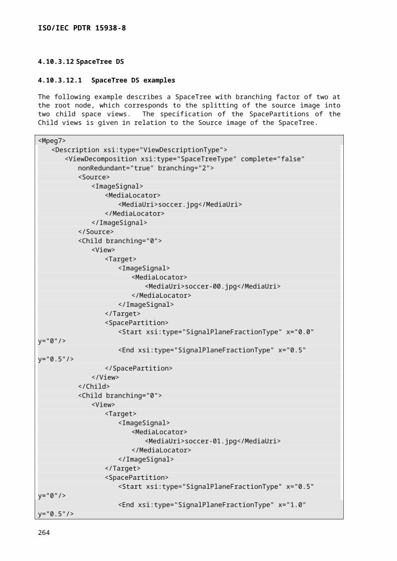
ISO/IEC PDTR 15938-8
20:17:30 0:08:28 View King of Queens 03-tkoq-000046
20:27:02 0:25:49 View Antiques Roadshow 08-ar-000123
20:53:02 0:05:15 View Tucker 03-tkr-000002
21:00:33 0:27:27 View Everybody Loves Raymond 03-elr-000074
21:12:35 0:03:51 Mute Everybody Loves Raymond 03-elr-000074
21:30:10 0:25:14 View Becker 03-bec-000062
21:55:00 1:10:00 Record Family Law 04-flw-000048
21:55:44 N/A Off N/A
23:04:10 N/A On N/A
23:04:27 0:18:14 View Channel 2 News 01-katu-100900:2300
23:24:01 0:08:15 View KOIN 6 News at 11 01-koin-100900:2300
23:34:20 0:25:40 View Late Show 06-lsdl-002321
4.12.3.1.3 UsageHistory DS use
In general, UsageHistory descriptions may be used directly for personalized searching, filtering and browsing, or may be mapped to a description of the user's preferences.
4.12.3.2 UserActionHistory DS
4.12.3.2.1 UserActionHistory DS examples
This example illustrates the use of the ObservationPeriod element to describe the time interval during which the accompanying user action history information was collected. The specified time interval can comprise multiple discrete observation periods. In this case, the user's activities were observed between 6PM-12PM PST on 10/09/2000 and 10/10/2000. The user would like to keep his identity protected, but does not mind distribution of his user action history to other parties.
<UsageHistory id="usage-history-002" allowCollection="true"><UserIdentifier protected="true">
<Name xml:lang="en">John Doe</Name></UserIdentifier><UserActionHistory id="useraction-history-001" protected="false">
<ObservationPeriod><TimePoint>2000-10-09T18:00-08:00</TimePoint><Duration>PT6H</Duration>
</ObservationPeriod><ObservationPeriod>
<TimePoint>2000-10-10T18:00-08:00</TimePoint><Duration>PT6H</Duration>
</ObservationPeriod><UserActionList>
<!-- user action list description (sequence of user actions) --></UserActionList>
</UserActionHistory></UsageHistory>
266

ISO/IEC PDTR 15938-8
4.12.3.3 UserActionList DS
4.12.3.3.1 UserActionList DS examples
The following example depicts two instantiations of the UserActionList DS as part of the UsageHistory, for "Record" and "PlayStream" actions. The example offers alternative representations of user actions by instantiating a subset of the available set of description schemes. Specifically, more comprehensive information is provided for the "Record" action, with each individual UserAction instantiated. For the "PlayStream" action, on the other hand, only the number of instances and the total duration is provided, which reduces the size of the description significantly. The description scheme allows differentiation between various types of actions, and provide the means for implementers to instantiate each action type in a specific way.
<UsageHistory id="usage-history-003" allowCollection="true"><UserIdentifier protected="true">
<Name xml:lang="en">John Doe</Name></UserIdentifier><UserActionHistory id="useraction-history-002" protected="false">
<ObservationPeriod><TimePoint>2000-10-09T18:00-08:00</TimePoint><Duration>PT6H</Duration>
</ObservationPeriod><UserActionList id="ua-list-001" numOfInstances="2"
totalDuration="PT2H30M"><ActionType href="urn:mpeg:mpeg7:cs:ActionTypeCS:2001:1.3">
<Name>Record</Name></ActionType><UserAction> <!-- user action description --> </UserAction><UserAction> <!-- user action description --> </UserAction>
</UserActionList><UserActionList id="ua-list-002" numOfInstances="25"
totalDuration="PT1H2M"><ActionType href="urn:mpeg:mpeg7:cs:ActionTypeCS:2001:1.2">
<Name>PlayStream</Name></ActionType>
</UserActionList></UserActionHistory>
</UsageHistory>
4.12.3.4 UserAction DS
4.12.3.4.1 UserAction DS examples
The following example highlights instantiations of the UserAction DS, and the functionality provided by the ActionTime DS. MediaTime and GeneralTime elements are different for user actions such as "Rewind," "FastForward" and "SlowMotion." For example, as shown in the example, a "FastForward" action that lasts only a few seconds in terms of general time may actually correspond to several minutes in terms of the media time base. Relying only on the general time to represent the time of occurrence and duration of an action may lead to inconsistencies and ambiguity. Thus the proposed syntax supports representation of ActionTime in terms of both media time and general time.
The ActionDataItem element can be used in two main capacities: (i) to refer to a specific part of a content description (such as the description of a segment that the user reviews in slow motion); and (ii) to provide a reference to related content material through the RelatedMaterial DS element of the CreationMetaInformation description scheme. In the first case, a usage history processor may, for example, use these references to keep local copies of the content description relevant to an action.
267

ISO/IEC PDTR 15938-8
An example of the second functionality is illustrated below for the "ClickThrough" action, where a user follows a URL that is defined as part of the RelatedMaterial description instance.
<UsageHistory id="usage-history-004" allowCollection="true"><UserIdentifier protected="true">
<Name xml:lang="en">John Doe</Name></UserIdentifier><UserActionHistory id="useraction-history-003" protected="false">
<ObservationPeriod><TimePoint>2000-10-09T18:00-08:00</TimePoint><Duration>PT6H</Duration>
</ObservationPeriod><ObservationPeriod>
<TimePoint>2000-10-10T18:00-08:00</TimePoint><Duration>PT6H</Duration>
</ObservationPeriod><UserActionList id="ua-list-003"
numOfInstances="2" totalDuration="PT2H30M"><ActionType href="urn:mpeg:mpeg7:cs:ActionTypeCS:2001:1.3">
<Name>Record</Name></ActionType><UserAction> <!-- user action description --> </UserAction><UserAction> <!-- user action description --> </UserAction>
</UserActionList><UserActionList id="ua-list-004"
numOfInstances="25" totalDuration="PT7H02M"><ActionType href="urn:mpeg:mpeg7:cs:ActionTypeCS:2001:1.2">
<Name>PlayStream</Name></ActionType><UserAction>
<ProgramIdentifier organization="MyIDOrg" type="MyIDType">01-mnf-100900
</ProgramIdentifier></UserAction><UserAction>
<ProgramIdentifier organization="MyIDOrg" type="MyIDType">02-mnf-100900
</ProgramIdentifier><ActionDataItem
href="www.abc.com/content/mnf/100900/mnf-stream.xml#segment_145"/>
</UserAction><!-- more user actions . . . -->
</UserActionList><UserActionList id="ua-list-005" numOfInstances="3"
totalDuration="PT4M20S"><ActionType href="urn:mpeg:mpeg7:cs:ActionTypeCS:2001:1.6">
<Name>FastForward</Name></ActionType><UserAction>
<ActionTime><MediaTime>
<MediaTimePoint>2000-10-09T19:10:12</MediaTimePoint><MediaDuration>PT1M45S</MediaDuration>
</MediaTime><GeneralTime>
<TimePoint>2000-10-09T19:10:12-08:00</TimePoint><Duration>PT8S</Duration>
</GeneralTime></ActionTime><ProgramIdentifier organization="MyIDOrg" type="MyIDType">
268

ISO/IEC PDTR 15938-8
02-mnf-100900</ProgramIdentifier><ActionDataItem
href="www.abc.com/content/mnf/100900/mnf-stream.xml#comm_break_17"/>
</UserAction><UserAction>
<ActionTime><MediaTime>
<MediaTimePoint>2000-10-10T18:16:08</MediaTimePoint><MediaDuration>PT1M35S</MediaDuration>
</MediaTime><GeneralTime>
<TimePoint>2000-10-10T18:16:08-08:00</TimePoint><Duration>PT7S</Duration>
</GeneralTime></ActionTime><ProgramIdentifier organization="MyIDOrg" type="MyIDType">
01-wnpj-101000</ProgramIdentifier><ActionDataItem
href="www.abc.com/content/news/101000/wnpj.xml#news-item-8"/>
</UserAction><UserAction>
<ActionTime><MediaTime>
<MediaTimePoint>2000-10-10T20:05:34</MediaTimePoint><MediaDuration>PT1M</MediaDuration>
</MediaTime><GeneralTime>
<TimePoint>2000-10-10T20:05:34-08:00</TimePoint><Duration>PT5S</Duration>
</GeneralTime></ActionTime><ProgramIdentifier organization="MyIDOrg" type="MyIDType">
03-tss-000063</ProgramIdentifier><ActionDataItem
href="www.fox.com/xml/that70sshow/063/tss-063.xml#break_2"/>
</UserAction></UserActionList><UserActionList id="ua-list-006" numOfInstances="1">
<ActionType href="urn:mpeg:mpeg7:cs:ActionTypeCS:2001:3.1"><Name>ClickThrough</Name>
</ActionType><UserAction>
<ActionTime><GeneralTime>
<TimePoint>2000-10-09T18:48:01-08:00</TimePoint></GeneralTime>
</ActionTime><ProgramIdentifier organization="MyIDOrg" type="MyIDType">
02-mnf-100900</ProgramIdentifier><ActionDataItem
href="www.abc.com/content/mnf/100900/mnf-stream.xml#rel_media_12"/>
</UserAction></UserActionList>
269

ISO/IEC PDTR 15938-8
</UserActionHistory></UsageHistory>
5 Visual tools
5.1 Basic visual tools
5.1.1 Grid Layout
The grid layout is a splitting of the image into a set of rectangular regions, so that each region can be described separately. Each region of the grid can be described in terms of other descriptors such as color, texture, or structure.
5.1.1.1 DDL instantiation examples
In the following example, Color Layout are instanciated and assigned at (0,1) and (1, 0).
<Grid Layout numOfPartX=”2” numOfpartY=”2” descriptorMask=”0110”><!--instance at (0 1) --><Descriptor xsi:type=”ColorLayoutType”>
<YDCCoeff>50</YDCCoeff><CbDCCoeff>34</CbDCCoeff><CrDCCoeff>30</CrDCCoeff><YACCoeff5>16 12 15 12 17 11</YACCoeff5><CbACCoeff2>12 17</CbACCoeff2><CrACCoeff2>12 14</CrACCoeff2>
</Descriptor><!--instance at (1 0) --><Descriptor xsi:type=”ColorLayoutType”>
<YDCCoeff>48</YDCCoeff><CbDCCoeff>34</CbDCCoeff><CrDCCoeff>32</CrDCCoeff><YACCoeff5>12 10 13 9 10 15</YACCoeff5><CbACCoeff2>14 15</CbACCoeff2><CrACCoeff2>16 12</CrACCoeff2>
</Descriptor></RegularTimeSeries>
5.1.2 Visual time series
The TimeSeries describes a temporal series of descriptors in a video segment and provides image to video-frame matching and video-frames to video-frames matching functionalities. Two types of TimeSeries are available: RegularTimeSeries and IrregularTimeSeries. These are useful in particular to build descriptors that contain time series of descriptors. Each of them basically consists of a series of descriptors and temporal intervals between them as illustrated in Figure 67. They corresponds the following two cases:
a. Descriptors locate regularly (with constant intervals) within a given time span.b. Descriptors locate irregularly (with various intervals) within a given time span.For the case a, specifying the temporal interval can be saved by means of introducing its default value. For the case b, the temporal interval can be associated with a descriptor by means of describing the series of (descriptor, time info.) pairs. However, it is apparently redundant for the case a. Therefore, separate tools are provided.
270

ISO/IEC PDTR 15938-8
one video segment
....
.D1 D2 D3 DnDn-1
I0 I1 I2 In-1 InI3
Time
Figure 67: Overview of the Time Series(1) RegularTimeSeries
RegularTimeSeries is appropriate to describe the time series in that descriptors locate regularly within a given time span. This enables a simple representation for the application that requires low complexity.
(2) IrregularTimeSeries
IrregularTimeSeries is appropriate to describe the time series in that descriptors locate irregularly within a given time span. This enables an efficient representation for the application that has the requirement of narrow transmission bandwidth or low storage capability.
5.1.2.1 Feature extraction
5.1.2.1.1 Regular visual time series
The extraction method of each descriptor should follows in the one of the assigned descriptor. Descriptors in the TimeSeries are extracted with the specified constant interval by starting on the specified time point offset. The offset is illustrated as “I0” in Figure 67. The constant interval between the descriptors is specified at the TimeIncr field in the RegularTimeSeries.
5.1.2.1.2 Irregular visual time series
The extraction method of each descriptor should follows in the one of the assigned descriptor. The extraction process consists of two steps:
Step 1: Extraction of the descriptor with fixed interval,
Step 2: Adaptive sub-sampling of the derived descriptors
Figure 68 illustrates these processes.
Time
TimeIncr
video segment
derived series ofdescriptors
sub-sampled series of descriptors
offset
271
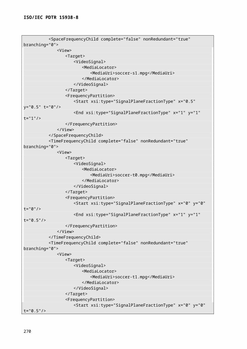
ISO/IEC PDTR 15938-8
Figure 68: Extraction method of a series of descriptorsThe first step is the repetition of the descriptor extraction process. Descriptors in the TimeSeries are extracted with the specified constant interval by starting on the specified time point offset. The offset is illustrate as “I0” in Figure 1. The constant interval between the descriptors is specified at the TimeIncr field in the IrregularTimeSeries. The derived series of descriptors will be sub-sampled as follows. The first descriptor is selected as a reference descriptor, and the following process is applied from the second descriptors. The derived descriptor is compared with its previous reference descriptor. If the difference is larger than threshold Th, the descriptor is set as a new reference descriptor. The time interval is derived as the number of merged descriptors. The collection of the descriptors selected as the reference descriptor form the description of the irregular time series, which is the adaptive sub-sampled series of the descriptor. Figure 69 shows the flow chart of the extraction of the time interval.
Figure 69: Flow chart to extract time intervals.
5.1.2.2 Similarity matching
The similarity of the two descriptor-values should be calculated as following the calculation method of the descriptor assigned in the RegularTimeSeries/IrregularTimeSeries. Here, the distance between two descriptor-values is denoted as Dist.
5.1.2.2.1 Regular visual time series
5.1.2.2.1.1 Image to sequence matching
The descriptor-value of the query image can be compared to each in the series easily. The distance between the image and each in the series is calculated as Dist. The most similar frame to the image can be derived by selecting the video frame whose distance is the minimum of all.5.1.2.2.1.2 Sequence to sequence matching
The similarity calculation method of two RegularTimeSeries, the longer one RTS1 and the shorter one RTS2 are defined as the following two cases:
(1) Two sets of series have the same value of TimeIncr
(2) Two sets of series have different values of TimeIncr
The most similar part of RTS1 to the RTS2 series can be derived by the clipped series whose distance is the minimum of all.
(1) The same TimeIncr value
When two sets of RegularTimeSeries have the same value of TimeIncr, the similarity calculation between them consists of the following two steps: Step 1: Candidate series clipping (clipping the longer RTS1 segment)
272

ISO/IEC PDTR 15938-8
The candidate series whose length is equal to the shorter RTS2 is clipped out of the longer RTS1 so that the number of descriptors in the candidate is as many as the shorter RTS2. Here, n denotes the number of descriptors.
Step 2: Similarity calculation between the RTS2 series and the clipped series
The distance between RTS2 and the clipped one can be defined as:
where Distl denotes the distance between the l-th descriptors in the series.Whole of the RTS1 series are scanned on the first step. The clipping of the candidate series starts from the beginning of the RTS1 series and continues to the end of the series by shifting a TimeIncr step.
(2) Different TimeIncr valuesOn the other hand, when two sets of RegularTimeSeries have different value of TimeIncr, each series should be converted into a new IrregularTimeSeries. The TimeIncr value of new IrregularTimeSeries is derived as the greatest common divisor between two values of the original series. In this case, the similarity calculation method is the same as that presented in Section 5.1.2.2.2 for comparison of two IrregularTimeSeries that have the same TimeIncr value.5.1.2.2.2 Irregular visual time series
5.1.2.2.2.1 Image to sequence matching
The descriptor-value of the query image can be compared to each in the series easily. The distance between the image and each in the series is calculated as Dist. The most similar frame to the image can be derived by selecting the video frame whose distance is the minimum of all.
5.1.2.2.2.2 Sequence to sequence matching
The similarity calculation method of two RegularTimeSeries, the longer one ITS1 and the shorter one ITS2 are defined as the following two cases:
(1) Two sets of series have the same value of TimeIncr
(2) Two sets of series have different values of TimeIncr
The most similar part of ITS1 to the ITS2 series can be derived by the clipped series whose distance is the minimum of all.
(1) The same TimeIncr value
When two sets of IrregularTimeSeries have the same value of TimeIncr, the similarity calculation between them consists of the following two steps: Step 1: Candidate series clipping (clipping the longer ITS1 segment)
The candidate series is clipped from the ITS1 series. Figure 70 shows an overview of this step. Summing up interval values in the stored video from a start position pos until the sum is over L, where L denotes the total intervals of ITS2 series, performs clipping. Then, similarity is calculated between the ITS2 series and the clipped segment in the next step.
273

ISO/IEC PDTR 15938-8
d0, l0 d1, l1 d2, l2
Candidate Series Clipping
Shorter seriesITS2
current first position(pair=0, pos=2)
L
+ (L0 - pos)
+ L1
+L2stop when SUM over L
SUM=0
Di, dj: descriptor valuesLi, lj: intervals
Time
D1, L'1D0, L'0 D2, L'2
.....D1, L1 D3, L3 D4, L4D0, L0 D2, L2
pair0 pair1 pair2 pair3 pair4
TimeIncr
Clipped Segment
Longer seriesITS1
Figure 70: Overview of video segment clipping Step 2: Similarity calculation between the ITS2 series and the clipped seriesIn this step, the ITS2 series and the clipped series are compared and series of distances will be calculated to derive the distance between them. Figure 71 shows an overview of this step. The distance Dist between two descriptors Di and dj should be calculated only on descriptor-value change points (comparison points). Therefore, similarity calculations between two descriptors could be reduced using IrregularTimeSeries. Also intervals in the series of distances are calculated between the change points.
D1, L'1D0, L'0 D2, L'2
d0, l0 d1, l1 d2, l2ITS2
Clipped Segment
Series of distances
Di, dj: descriptor valuesLi, lj: intervals
Dur0 Dur1 Dur2 Dur3 Dur4
Dist0
Dist1
Dist2
Dist3
Dist4
Comparisonpoints
Time
TimeIncr
Figure 71: Overview of similarity calculation between two IrregularTimeSeries.
The distance between two sets of IrregularTimeSeries should be calculated as follows:
Here, Distl denotes the distance between descriptors on the l-th comparison point, Durl denotes the l-th interval following the l-th comparison point, m denote the number of comparison points and L denotes the time length (total intervals) of the ITS2 series.
Whole of the ITS1 series are scanned on the first step. The clipping of the candidate series starts from the beginning of the ITS1 series and continues to the end of the series by shifting a TimeIncr step.
274

ISO/IEC PDTR 15938-8
These two steps explained above are equivalent to the following C-like pseudo codes. Let the ITS2 series be {(d(i), l(i)): i=0,1,…,I-1}}, where d denotes the descriptor value and l denotes the interval value, respectively. The ITS1 series is denoted as {(D(j), L(j)): j=0,1, …, J-1}.
double DistanceofSeries(d, l, I, D, L, J){int i=j=0; double Sum=0; int len=0; int dur;Descriptor des, Des;int interval, Interval;des=d(i), interval=l(i), Des=D(i), Interval=L(i)do {
// Select shorter one to find a change point sequentially in temporal ascending order dur=minimum(interval, Interval) len=len+dur; Sum+=Distance(des, Des); // Distance between two descriptors if( (interval=interval-l)==0 ) { i++;
if(i==I) break; // reached the end of the query des=d(i); interval=l(i); } if( (Interval=Interval-l)==0 ){
j++;if(j==J) break; // reached the end of the clipped segmentDes=Des(j); Run=T(j);
}} while( 1 );return Sum=Sum / len;
}
(2) Different TimeIncr valuesOn the other hand, when two sets of IregularTimeSeries have different values of TimeIncr, each series should be converted into a new IrregularTimeSeries. The TimeIncr value of new two IrregularTimeSeries is derived as the greatest common divisor between two values of the original series. In this case, the similarity calculation method is the same as that presented above for comparison of two IrregularTimeSeries that have the same TimeIncr value.
5.1.2.3 Conditions of usage
Selection of RegularTimeSeries and IrregularTimeSeriesThe usage depends on applications. The IrregularTimeSeries has an advantage in the transmission/storage cost. This is appropriate to the application that has the requirement of narrow transmission bandwidth or low storage capability because it enables an efficient description. On the other hand, the RegularTimeSeries have a different advantage, which is in its easy handling capability. If two temporal series of elemental visual descriptors have the regular structure (with the same constant time intervals), it is easy to calculate the similarity between the temporal series since there are no needs to consider about the difference of temporal positions. This is appropriate for a simple representation to the application that requires low complexity.
Appropriate descriptor assigned to the TimeSeries
The TimeSeries (binary version) assumes that only the descriptor identifier and the descriptor length are the common information of the series. Therefore, it is appropriate for descriptors of which the size is constant.
TimeIncr
The value of TimeIncr should be the same between the query series and the target series, because of the lower complexity of similarity calculation and easy handling capability. For example, in the case of ColorLayout descriptor, each descriptor should be extracted under the condition of:
TimeIncr is equal to 2 frame per second (every 0.5second), Th is equal to 3
275

ISO/IEC PDTR 15938-8
This condition gives the best retrieval performance with efficient transmission/storage cost.
5.1.2.4 DDL instantiation examples
5.1.2.4.1 Regular visual time series
The description of a series of MyDescriptor located at 0.0s, 0.2s, 0.4s, 0.6s, 0.8s within a time span [0.0s,1.0s] becomes:
<RegularTimeSeries><TimeIncr timeUnit="PT2N10F">1</TimeIncr><MyDescriptor> ... </MyDescriptor><MyDescriptor> ... </MyDescriptor><MyDescriptor> ... </MyDescriptor><MyDescriptor> ... </MyDescriptor><MyDescriptor> ... </MyDescriptor>
</RegularTimeSeries>If the locations of MyDescriptor are at 0.1s, 0.4s and 0.7s then the description becomes:
<RegularTimeSeries><offset timeUnit=”PT1N10F”>1</offset><TimeIncr timeUnit="PT3N10F">1</TimeIncr><MyDescriptor> ... </MyDescriptor><MyDescriptor> ... </MyDescriptor><MyDescriptor> ... </MyDescriptor>
</RegularTimeSeries>
5.1.2.4.2 Irregular visual time series
The description of series of MyDescriptor located at 0.0s, 0.4s, 0.5s, 0.8s and 0.9s within a time span [0.0s,1.0s] becomes:
<IrregularTimeSeries><TimeIncr timeUnit="PT1N10F">1</TimeIncr><MyDescriptor> ... </MyDescriptor><Interval>4</Interval><MyDescriptor> ... </MyDescriptor><Interval>1</Interval><MyDescriptor> ... </MyDescriptor><Interval>3</Interval><MyDescriptor> ... </MyDescriptor><Interval>1</Interval><MyDescriptor> ... </MyDescriptor><Interval>1</Interval>
</IrregularTimeSeries>Note that the interval must be always specified for each descriptor in this tool.
5.1.3 2D-3D multiple view
The 2D/3D Descriptor specifies a structure which combines 2D Descriptors representing a visual feature of a 3D object seen from different view angles. The descriptor forms a complete 3D view-based representation of the object. Any 2D visual descriptor, such as for example contour-shape, region-shape, colour or texture can be used. The 2D/3D descriptor suports integration of the 2D descriptors used in the image plane to describe features of the 3D (real world) objects.
5.1.3.1 Feature extraction
The following Figure 72 shows an example of 7 views for the object “Bicycle-1”. The viewing directions, associated with these views, have proven to give good retrieval results, if a Contour
276

ISO/IEC PDTR 15938-8
Descriptor is used, that provides invariance to mirrored shapes, and the extracted features for front and back view are identical.
Figure 72: Different views of model “Bicycle-1.wrl”: Top: pri., sec. and ter. View, Bottom: Intermediate views 4, 5, 6 and 7
For obtaining typical views from the 3D object, the following approach is recommended:
The primary, secondary and tertiary viewing directions are determined by the analysis of the covariance matrix of the 3D object
where
are the coordinates of all volume elements and the mass center of the 3D object, respectively, and N is the number of volume elements. An Eigenvector analysis is now performed, where the Eigenvalues 1-3 are associated with primary, secondary and tertiary views, and the corresponding Eigenvectors p1-p3 indicate the view directions:
with ,
In the case of a Contour-based shape description, another 4 views are added addition to these3 views,with the following directions to obtain object coverage with most spatial distance:
View_4 45° between Primary and Secondary view
View_5 45° between Primary and Tertiary view
View_6 45° between Secondary and Tertiary view
277

ISO/IEC PDTR 15938-8
View_7 45° between Primary, Secondary and Tertiary view
Figure 73 shows the position of all generated views. For the similarity search by shape, only the hemisphere y>0 needs to be considered. Respective views in other octants would only
yield mirrored shapes of the 7 available views.
Figure 73: Viewing directions onto the 3D object in the origin: Left: perspective view and view directions in the first octant, Right: top view and view directions in the hemisphere y>0.
In the case of other underlying descriptor, e.g. color or texture, arbitrary views are recommended, since front and back view of an object may no longer yield identical descriptor values. An example of the arbitrary views is shown on Figure 74. Arbitrary views can be used in the representation of 3D objects contained within photographs and movie sequences, when obtaining views from the fixed directions is impractical or impossible.
Figure 74: The construction of a multi-view descriptor of a real 3D car.
5.1.3.2 Similarity matching
Matching can be achieved by comparing a number of views of one object (A) to the same number of views of the other object (B), using the matching procedure of the underlying Image Descriptor in the following way:
x
z
y
3
2 4
1
z
x
1
6
7
5
4
3
2
278

ISO/IEC PDTR 15938-8
Each view from A is compared to each view from B, giving N2 matching results, if N was the number of used views. The overall matching error is obtained by adding the underlying error measures of all possible view combinations between A and B.
This procedure can also be described by the Error Matrix E between Object A and B, where each matrix element ek,l represents the underlying error measure between the k th view of object A and the lth
view of object B. Finding the overall matching error is similar to calculating the smallest trace of all possible column changes of E.
As an example, the following 6 column changes and resulting traces are possible when using 3 views:
e1,1+e2,2+e3,3 e1,1+e2,3+e3,2 e1,2+e2,1+e3,3 e1,2+e2,3+e3,1 e1,3+e2,1+e3,2 e1,3+e2,2+e3,1
The minimum of the 6 traces (sums) listed below the possible column-arranged error matrix represents the overall matching error.
A second matching approach is to compare an unknown 2D view with the 3D object. Here the descriptor of the unknown 2D view is compared to each view of the 3D object seperately and the minimum error represents the similarity between unknown 2D view and 3D object.
5.1.3.3 Visible views
The multi-view descriptor contains a number of descriptors that represent an object from different views. It is also nessesary to describe which of these views are actually visible from within the image or sequence of images that the multi-view description object relates to. Figure 75 gives an example of a car object within a photo-graph being described using the multi-view descriptor, and a visibility flag for each of the views. Figure 76 shows how the visible flags can affect the search results obtained from a multi-view search. Figure 76 (a) shows a search using a side view of a car without using the visible flags: it finds pictures of cars with a similar side views though they are not nessasarly visible from the photo. If the person performing the search wishes to view only side views of cars it is not possible without the use of the visible view flag. Figure 76 (b) shows the same search but this time the visible flags are being used. The results contain only side views of cars.
279

ISO/IEC PDTR 15938-8
Figure 75: An example of a multi-view descriptor using shape including visible view information
(a) Without the visible view flag the multi-view search finds car from any angle.
(b) Using the visible views flag the search returns only the required side views.
Figure 76: Visible view flag usage
5.1.3.4 Conditions of use
When the multiple-view descriptor is used to describe an object within an image or movie frame it is recomended that the descriptor be inserted into the MPEG 7 framework via the StillRegionDS.
5.1.4 Spatial 2D coordinates
This description defines a 2D spatial coordinate system and a unit to be used by reference in other Ds/DSs when relevant. The coordinate system is defined by a mapping between an image and the coordinate system. One of the advantages using this descriptor is that MPEG-7 descriptions need not to be modified even if the image size is changed or a part of the image is clipped. In this case, only the description of the mapping from the original image to the edited image is required.
It supports two kinds of coordinate systems: “local” and “integrated” (Figure 77). In a “local” coordinate system, the coordinates used for the calculation of the description is mapped to the current coordinate system applicable. In an “integrated” coordinate system, each image (frame) of e.g. a video may be mapped to different areas with respect to the first frame of a shot or video. So, integrated coordinate system can for instance be used to represent coordinates on a mosaic of a video shot.
a) “Local” coordinates b) “Integrated” coordinates
Figure 77: “local” and “integrated” coordinate system In the normative syntax, IntegratedCoordinateSystem allows to specify an integrated coordinate system, and LocalCoordinateSystem allows to specify a local one, when it is different from the default local coordinate system. The default local coordinate system is the pixel based coordinate system whose origin is placed at the top left corner of the image and whose first and the second axis are aligned to the horizontal respectively vertical boarder of the image with increasing indixes to the right respectively bottom of the image. Thus a LocalCoordinateSystem provides the possibility to map a
280

ISO/IEC PDTR 15938-8
default local coordinate system which was used to compute visual descriptors to the coordinate system of the current image or video transmitted or rendered. By referencing this mapping, the visual descriptors have not to be recomputed even though e.g. the format of the current image or video has changed. The specification of the local coordinate system is applicable for images or video. If additionally an Integrated coordinate system is specified, the mapping applies to the coordinate system of the first frame.
5.1.4.1 Conditions of use
As mentioned above, the Spatial2DcoordinateSystem description can be referenced in Ds/DSs instantiating coordinates. This reference is optional, driven by a 1-bit flag in all the relevant Ds/DSs. If the Spatial 2D Coordinate System is not referenced, all relevant Ds/DSs have embedded all the data they need to be used in most usual basic cases. If it is referenced, further advanced functionalities and advantages are possible. We describe below these advantages and functionalities, and the cases in which we recommend to reference the Spatial 2D Coordinates System.
Flexibility with respect to the media format which is describedFor the so called universal multimedia access applications (UMA) the multimedia contentn has to be adapted to the user device or to different bandwidth conditions. In these contexts, resizing and cropping of the visual content are common adaptation mechanisms, beside several others. The resizing is depicted in Figure 78.
Without referencing the Spatial2DcoordinateSystem, two notions of embedded coordinate systems are used in Ds/DSs instantiation coordinates:
- Normalized coordinates: the coordinate specification is normalized to the image size.- Pixel coordinates: the coordinates refer to the pixel position within an image or frame, the origin
lying in the upper left corner.After applying a resize operation, the coordinates in a normalized coordinate system maintain valid while the ones in a pixel-based coordinate system are not correct anymore. In the case of the cropping operation, Ds/DSs making use of any of these coordinate systems have to be recomputed. So in the
Figure 78: Coordinate changes by scaling of an image: original descriptor in the src coordinate system and its mapping into the target coordinate system (in this example
both pixel based)
281

ISO/IEC PDTR 15938-8
majority of the cases the spatial descriptions which are assuming one of these implicit coordinate systems have to be recomputed to stay valid with respect to the transmitted data. If we specify a coordinate system which relates the spatial description to the image or video delivered (e.g. see Figure 78), only the coordinate system has to be changed. The remaining description stays the same, and always uses the original pixel or normalized coordinates (src coordinate system in Figure 78). These coordinates are mapped to the pixel coordinates of the modified image or video (current coordinate system in Figure 78). For retrieval the mapping does not have to be applied. The descriptor with respect to the src coordinate system can be used as it would be the case for the original image without the spatial 2D coordinate system. In the example of Figure 78 the resizing of the image can be described by the following spatial 2D coordinate system.
<Spatial2DCoordinateSystem " xRepr="16" yRepr="16" xSrcSize="384" ySrcSize="256" id="SCSNewImg1">
<LocalCoordinateSystem name="PixelCoords"><CurrentPixel>0 0</CurrentPixel><SrcPixel>0 0</SrcPixel><CurrentPixel>150 100</CurrentPixel><SrcPixel>300 200</SrcPixel>
</LocalCoordinateSystem></Spatial2DCoordinateSystem>
In this example the mapping between the pixels of the src coordinate system and the pixels of the current coordinate system are specify as a downscaling of factor 2.
Generalized approach to global motionWhen there is a global motion in a scene, which has been calculated as a sequence of parametric motion parameters, referencing the Spatial2DCoordinateSystem allows storing this information using the IntegratedCoordinateSystem element. All Ds/DSs referencing the Spatial2DcoordinateSystem can access the global motion information.
Then, a 1-bit flag in each D/DS referencing the Spatial2DcoordinateSystem specifies whether the coordinate values are given with respect to the local coordinate system, or with respect to the integrated one. This bit should be chosen depending on the targeted application. It allows coordinate values to be accessed in a form, which is directly useful for the application.
For instance, let us assume that an IntegratedCoordinateSystem has been defined for a segment of a sport sequence where the camera is moving. Then, if the application wants to offer object hyperlinking, it is useful to directly access the image-local coordinates of the object, as the cursor coordinates are also known in the image. On the contrary, if the application proposes similarity-based retrieval taking into account object motion, it is useful to have direct access to the coordinates in the Integrated CS, as they represent object behaviors independently from the movements of the camera.
5.1.5 Temporal interpolation
5.1.5.1 Feature extraction
The algorithm CALC_INTERPOLATION gives an example of key points extraction method for variable key point intervals. It determines key points sequentially based on the approximation error of interpolation functions.
In the algorithm, the interpolation is initialized with the first two points. The interpolation is then widened to include one point at a time until the approximation error of the interpolation becomes larger than a given threshold. At that point a new key point is added and a new interpolation interval is started with the new key point (starting point) and the immediately following point (ending point). This procedure is interated until all points have been processed. When the interpolation models matches the variable values well, this algorithm results in a small number of long intervals. Conversely, when the match is poor, a large number of short intervals will result.
282

ISO/IEC PDTR 15938-8
To describe the algorithm formally, define the following notation. Let be the number of variables (dimension) and denote the value of the -th variable at time by . A
series of time points is denoted by . For a (candidate) interpolation interval, the starting
time (ending time) is denoted by ( ). Let be a candidate of
the -th variable interpolation function. This can be calculated using least squares. In this case,
is calculated to minimize
.
This calculation is easy because the function is a first or the second order polynomial. To evaluate the derived candidate function, let to be a threshold for the -th variable and define error
as
.
is the maximum approximation error of the -th variable in the range . If
holds for all , is an acceptable candidate. However, another interpolation function in wider interval may be found. To try to test this possibility, the interval is widened by incrementing END and a new function is derived and tested. This procedure is repeated until a newly derived function doesn ’t meet the acceptance condition. Then, the last candidate function is accepted and both edges of the interval are fixed as key points.
The following are the steps of the algorithm.
CALC_INTERPOLATION:
1. (Initialization) Set , .
2. (Interpolation Calculation) Calculate interpolation functions . Least
square estimation can be used under conditions of and
.
3. (Interpolation Evaluation) Compute the maximum approximation error . If there exists which is greater than the corresponding threshold, go to Step 4. Otherwise, go to Step 5.
4. (KeyPoint Insertion) Accept as interpolation functions and set .
5. (Increment and Termination) If is the end of the whole interval, terminate the procedure. Otherwise, set and go to Step 2.
283

ISO/IEC PDTR 15938-8
Figure 79: Sequential key points selection and interpolation calculation method: If the error of is greater than the threshold, let be a key point and accept .
Otherwise, keep the new function as a candidate and discard the old function.
5.1.5.2 Decoding
In the following, the procedure to get a value of a temporal interpolation at a given time is explained. Let NumOfKeyPoints be the number of key points and t0 be the given time, Then, define T[i] (0<=i<NumOfKeyPoints) as the array of the key point time and V[i] (0<=i<NumOfKeyPoints) as the array of the key point values in the description.
1. Find i0 (0<=i0<NumOfKeyPoints-1) such that T[i0]<=t0<=T[i0+1]. If there are two i0 satisfying the condition, choose the smaller one. If there doesn’t exist i0 satisfying the condition, terminate the procedure and return false value.
2. According to the interpolation type of the interval T[i0]<=t<=T[i0+1], calculate the coefficient va
using ta=T[i0], tb=T[i0+1], fa=V[i0], fb=V[i0+1] and aa=param based on the equations in Table 3 inISO/IEC 15938-3.
3. Calculate f(t0) in the table and return the value.
5.1.5.3 DDL instantiation examples
In the following example, the position in 2D (x and y axes) is described by the TemporalInterpolation D, which is used in the MotionTrajectory Descriptor. Since four key points are used in the example, four key point positions and three interpolation functions for each axis are described. All the key points and the interpolation functions are shown in the table. For the y-axis only the default functions (first order polynomials) are used for the interpolation function, so the descriptions of type are omitted.
When TwoDimMotionTrajectory is defined as:
<element name="TwoDimMotionTrajectory" type="mpeg7:TemporalInterpolationType" />
then the description can be given as:
<TwoDimMotionTrajectory><!-- time of 4 key points --><KeyTimePoint>
<MediaTimePoint>T00:00:00:0F10</MediaTimePoint>
284
ISO/IEC PDTR 15938-8
<MediaTimePoint>T00:00:02:0F10</MediaTimePoint><MediaTimePoint>T00:00:10:5F10</MediaTimePoint><MediaTimePoint>T00:00:15:00F10</MediaTimePoint>
</KeyTimePoint>
<!-- X values of 4 key points --><InterpolationFunctions>
<KeyValue type="startPoint>118.9</KeyValue><KeyValue type="secondOrder" param=”2.1”>102.1</KeyValue><KeyValue type="firstOrder">82.35</KeyValue><KeyValue type="secondOrder" param=”0.2”>85.5</KeyValue>
</InterpolationFunctions><!-- Y values of 4 key points --><InterpolationFunctions>
<KeyValue>210.0</KeyValue><KeyValue>220.8</KeyValue><KeyValue>228.9</KeyValue><KeyValue>215.1</KeyValue>
</InterpolationFunctions></TwoDimMotionTrajectory>
Figure 80: Key points and interpolation functions used in this example. Red colored numbers, which are necessary to derive interpolation functions, can be found in the above description.
t
0.0 0.0 <= t <= 2.0 2.0 2.0 <= t <= 10.5 10.5 10.5 <= t <= 15.0 15.0
x 118.9 x=2.1t2-12.6t+118.9 102.1 x=-2.3t+106.73 82.35 x=0.2t2-4.4t+106.5 85.5
y 210.0 y=5.4t+210.0 220.8 y=0.95t+218.89 228.9 y=3.07t+261.13 215.1
Figure 81: The MotionTrajectory described in this example.When the interval between the key points is constant, then we can obtain a description as:
<TwoDimMotionTrajectory><WholeInterval>
<MediaDuration>PT15S</MediaDuration></WholeInterval>
285

ISO/IEC PDTR 15938-8
<!-- X values of 4 key points --><InterpolationFunctions>
<KeyValue type="startPoint>118.9</KeyValue><KeyValue type="secondOrder" param=”2.1”>102.1</KeyValue><KeyValue type="firstOrder">82.35</KeyValue><KeyValue type="secondOrder" param=”0.2”>85.5</KeyValue>
</InterpolationFunctions><!-- Y values of 4 key points --><InterpolationFunctions>
<KeyValue>210.0</KeyValue><KeyValue>220.8</KeyValue><KeyValue>228.9</KeyValue><KeyValue>215.1</KeyValue>
</InterpolationFunctions></TwoDimMotionTrajectory>
5.2 Color description tools
This section describes all the entities that describe visual features related to color.
5.2.1 Color space
The feature is the color space that is to be used in other color based descriptions.
In the current description, the following color spaces are supported:
- RGB
- YCbCr
- HSV
- HMMD
- Linear transformation matrix with reference to R, G, B
- Monochrome
5.2.1.1 DDL instantiation examples
Example 1: HMMD color space is defined by the Color space descriptor.
<ColorSpace type = “HMMD”/>
Example 2: The Color space descriptor describes a linear matrix transformation between the components (C1, C2, and C3) of an arbitrary color space and the components of the RGB color space.
C1 = ColorTransMat[0][0]*R + ColorTransMat[0][1]*G + ColorTransMat[0][2]*B;C2 = ColorTransMat[1][0]*R + ColorTransMat[1][1]*G + ColorTransMat[1][2]*B;C3 = ColorTransMat[2][0]*R + ColorTransMat[2][1]*G + ColorTransMat[2][2]*B.
Suppose the linear matrix (ColorTransMat) is specified as follows:
ColorTransMat[0][0] = 0.299;ColorTransMat[0][1] = 0.587;
286

ISO/IEC PDTR 15938-8
ColorTransMat[0][2] = 0.144;ColorTransMat[1][0] = -0.169;ColorTransMat[1][1] = -0.331;ColorTransMat[1][2] = 0.5;ColorTransMat[2][0] = 0.5;ColorTransMat[2][1] = -0.419;ColorTransMat[2][2] = -0.081;
In this matrix specification, each coefficient of the matrix is expressed a real number between –1 and 1. To convert the real number into a coded value (16 bit unsigned integer), the following equation is used.
Vint = Vfp*2^14.
Therefore, coded values of the coefficients are
ColorTransMat[0][0]_coded = 4898;ColorTransMat[0][1]_coded = 9617;ColorTransMat[0][2]_coded = 2359;ColorTransMat[1][0]_coded = –2769;ColorTransMat[1][1]_coded = –5424;ColorTransMat[1][2]_coded = 8192;ColorTransMat[2][0]_coded = 8192;ColorTransMat[2][1]_coded = –6865;ColorTransMat[2][2]_coded = –1328.
These coeffiecients of the linear matrix are described by the Color space descriptor as follows:
<ColorSpace type = “LinearMatrix”><ColorTransMat>4898 9617 2359 –2769 –5424 8192 8192 –6865 –1328</ColorTransMat>
</ColorSpace>
5.2.2 Color quantization
This descriptor defines the uniform quantization of a color space when the color space is quantized uniformly in all the color components to be quantized.
5.2.2.1 DDL instantiation examples
In the following example, a uniform quantization is described by color quantization descriptor in which each of H, Diff, and Sum component of HMMD color space is uniformly quantized by 256 levels.
<ColorQuantization><Component> H </Component><NumOfBins> 256 </NumOfBins><Component> Diff </Component><NumOfBins> 256 </NumOfBins><Component> Sum </Component><NumOfBins> 256 </NumOfBins>
</ColorQuantization>
5.2.2.2 Conditions of usage
Color quantization descriptor is used for describing a uniform color quantization of a color space specified in the color space descriptor. Non-uniform color quantization is not supported by the current description. If the defined color space is a linear matrix in the color space descriptor, any three arbitrary components are used in the color quantization descriptor to define the number of bins. Each number of bins of the three arbitrary components corresponds to that of C1, C2, and C3, respectively.
287

ISO/IEC PDTR 15938-8
5.2.3 Dominant color
This descriptor specifies a set of dominant colors in any arbitrary shaped region.
It targets content-based retrieval for color, either for the whole image or for any arbitrary shaped region (rectangular or irregular).
5.2.3.1 Feature extraction
The dominant color extraction algorithm takes as input a set of pixel color values (specified in the RGB color space). It quantizes the color vectors in the image based on the Generalized Lloyd Algorithm (GLA).
Note: In this section, several references are made to CIE LUV color space. All informations on this color space can be found in the following references:
C.A. Poynton “A technical introduction to Digital Video”, John Wiley, 1996 (in particular conversion formulas from RGB to CIE XYZ) A.K. Jain “Fundamentals of Digital Image Processing:, Prentice Hall, 1989 (in particular conversion formulas from CIE XYZ to CIE LUV) R.W.G. “The reproduction of Color”, 5th ed., Fountain Press, 1995 (fundamentals on color without conversion formulas)
The dominant colors are extracted as a result of successive divisions of the color clusters with the GLA algorithm in between each division and then merging of the color clusters. The detailed algorithm is explained in the following.
Note on the notation;Each color cluster center will be called the colorBin, and the number of Bins will be denoted as BinNum. So, the initial number of Bins will be denoted by the InitBinNum, the final number of Bins will be denoted by FinalBinNum, etc. Also each color will have an unique index, called IndexOfColor , and this indicate the Bin that the color is associated to..
1. Convert the color in an input image from RGB space to CIE LUV space.
2. Set InitBinNum=1, FinalBinNum=15, and CurrentBinNum = InitBinNum (4 bits)
3. Apply the GLA algorithm to the set of CurrentBinNum color clusters.
assign each color to its cluster for ( i=0; i<NumOfColors; i++ ) {
for ( j=0; j<CurrentBinNum; j++ )
distance[j] = EuclideanDistance (color[i],colorBin[j]);
IndexOfColor[i] = IndexOf (Minimum (distance) );
}
calculate cluster centroid for ( j=0; j<CurrentBinNum; j++ ) {
for ( i=0; i<NumOfColors; i++ )
288

ISO/IEC PDTR 15938-8
if ( IndexOfColor[i] == j ) colorBin[j] = colorBin[j] + color[i];
colorBin[j] = colorBin[j] / NumOfColorInBinJ;
}
4. Calculate the total distortion and split colorBins to increase CurrentBinNum until CurrentBinNum = FinalBinNum.
for ( i=0; i<NumOfColors; i++ )
Distortion = Distortion + SquareofL2Norm (colorBin[IndexOfColor[i]] - color[i]);
if ( Change in Distortion > 5% ) Repeat Step 3;
else {
Split colorBins using Step 5;
CurrentBinNum = CurrentBinNum +1;
if ( CurrentBinNum < FinalBinNum ) Repeat Step 3;
else Out of GLA loop and Goto Step 6;
}
5. One colorBin is split into two colorBins. The old one is discarded.
NewcolorBin1 = OldcolorBin + PerturbanceVector;
NewcolorBin2 = OldcolorBin - PerturbanceVector;
6. Merge colorBins using an agglomerative clustering method.
calculate mutual distances between codevectors for ( i=0; i<FinalBinNum; i++ ) {
for ( j=0; j<FinalBinNum; j++ )
DistanceTable[i][j] = distance (colorBin[i],colorBin[j]);
}
minimumDist = Minimum (DistanceTable);
merge two color bins with the smallest distance and update table; the Threshold is set to 255.0 for CIE LUV space
while ( minimumDist<Threshold ) {
NewColor = PercentOfColorsInI*ColorBin[i] + PercentOfColorsInJ*ColorBin[j];
Update DistanceTable;
289

ISO/IEC PDTR 15938-8
minimumDist = Minimum (DistanceTable);
}
7. Convert colorBins from CIELUV to RGB.
8. Quantize ColorBins to Dominant Colors using the feature descriptor syntax.
9. If the ColorVariances are required, calculate distortion components per dominant color as follows:
for ( i=0; i<NumOfColors; i++ ) { index=IndexOfColor[i]; for ( c=0; c<NumOfColComponents; c++ ) ColorVariance[index][c] += (colorBin[index][c]-color[i][c])*( colorBin[index][c]-color[i][c]);
}
for ( j=0; j<NumOfDominantColors; j++ ) for ( c=0; c<NumOfColComponents; c++ ) ColorVariance[j][c] /= NumberOfPixels[j];
and quantize it using the feature descriptor syntax.
5.2.3.1.1 Spatial coherency extraction:
The SpatialCoherency (SC) can be calculated as follows:
SC = for all i(COH_Ci × COUNT_PELS_Ci / TOTAL_PELS_OF_R)
where COH_Ci is the per-dominant color spatial coherency of Ci, COUNT_PELS_Ci is the number of corresponding pixels of Ci in the region R and TOTAL_PELS_OF_R is the size of the region R calculated by counting pixels in the region R.
Algorithm to calculate SpatialCoherency (SC) is described as follows:
1 Set SC = 0.
2 Set SUM_COUNT_PELS = 0.
3 For all pixels p in R
3.1 VISITED PELp=FALSE;
4 For all Dominant Colors Ci.
4.1 Get COH_Ci and COUNT_PELS_Ci.
4.2 SC = SC + COH_Ci×COUNT_PELS_Ci.
5 SC = SC / TOTAL_PELS_OF_R.
6 Output SC.
290

ISO/IEC PDTR 15938-8
In 3.1, COH_Ci (per-dominant color spatial coherency of Ci) and COUNT_PELS_Ci are calculated as follows:
1 Input the size of the Coherency Checking Mask (CCM) such as CCM_WIDTH (=3) by CCM_HEIGHT (=3).
2 COUNT_PELS_Ci = 0, TOTAL_NUM_COHERENT = 0.3 For all pixels PELj in R,
3.1 If (Ci == COLOR_OF_PELj & VISITED_PELj == FALSE)3.1.1 VISITED_PELj = TRUE;3.1.2 COUNT_PELS_Ci = COUNT_PELS_Ci +1.
// align PELj with center of CCM to check 8-connectedness connectivity as follows
3.1.3 For all masked pixels MASKED_PIXELk (except the center pixel, PELj)3.1.3.1 If (Ci == COLOR_OF_MASKED_PIXELk)
3.1.3.1.1 TOTAL_NUM_COHERENT ++; 4 COH_Ci = TOTAL_NUM_COHERENT / COUNT_PELS_Ci / (CCM_WIDTH * CCM_HEIGHT-1)5 Output COH_Ci and COUNT_PELS_Ci.5.2.3.2 Similarity matching
The following describes a matching method using the dominant color(s) descriptor.
Difference(D1, D2) = W1*SC_Diff *DC_Diff + W2*DC_Diff.
Where SC_Diff = abs(SpatialCoherency_1 – SpatialCoherency_2), SpatialCoherency_1 and SpatialCoherency _2 are normalized from 0 to 1 and non-uniformly quantized in prior to calculate SC_Diff. DC_Diff is the difference between two set of dominant colors, W1 (e.g. set to 0.3) is the weight of the first term and W2 (e.g. set to 0.7) is the weight of the second term. Set W1 to 0 if SpatialCoherency is not available.
DC_Diff, normalized from 0 to 1, can be computed by the following distance function:
For clarity, these notations corresponding to the descriptor syntax (normative parts) are used:
F: Dominant_Color N: DominantColorsNumber c: ColorValue p: Percentage. Percentage values are normalized to 1, i.e., . This means that, if the original sum does not add up to 100%, the rest of the colors are completely ignored.
The similarity between two feature descriptions, F1 and F2, can be measured by the following distance function D(F1, F2)
where the subscripts 1 and 2 in all variables stand for descriptions F1 and F2 respectively, and ak,l is the similarity coefficient between two colors ck and cl,
where dk,l is the Euclidean distance between two colors ck and cl,
291

ISO/IEC PDTR 15938-8
Td is the maximum distance for two colors to be considered similar, and dmax = Td. A normal value for Td is between 10-20 in the CIE LUV color space and for is between 1.0-1.5.
The procedure to calculate D(F1,F2) is as follows:
Step 1: Calculate the 2 positive squared terms in the distance function. Step 2: Take either color feature description, say F1, as the reference. For each color in F1, find all its similar
colors in F2, i.e., the colors that have distance less than Td. Step 3: Calculate the similarity coefficients and the negative term in the distance function.
If color variances are present, the following similarity measure is used:
where
and
In the equations above, cxil and vxil are dominant color values and color variances, respectively.
The above matching method assumes that the feature description is extracted using the method described in section 3.2.2.1. of this document. In particular, this means that any two dominant colors from one single description are at least Td distance apart.
5.2.3.3 Conditions of usage
The dominant color descriptor is useful for image and video retrieval. It targets content-based retrieval for color, either for the whole image or for any arbitrary shaped region (rectangular or irregular). It is a very compact descriptor, requiring less than 6-8 colors per region. Since colors are not pre-quantized as in the histogram type color descriptors, the representation is more accurate. It is intended for applications that use object based representations (objects or regions in an image).
5.2.4 Scalable color
The Scalable Color Descriptor is a Color Histogram in HSV Color Space, which is encoded by a Haar transform. Its binary representation is scalable in terms of bin numbers and bit representation accuracy over a broad range of data rates.
5.2.4.1 Feature extraction
The feature extraction consists of a histogram extraction in HSV color space, uniformly quantized into 256 bins according to the tables provided in the normative parts, and histogram values then nonlinearly quantized (according to Tables 4 in the normative parts)[Editor’s comments: need checking the correspondence with FDIS]. The 4-bit values then undergo a Haar transform according to flow
292

ISO/IEC PDTR 15938-8
diagrams in Figure 82, which is the forward transform compatible to the inverse transform described in the normative parts.
++
+-
++
+-
++
+-
++
+-
++
+
-
...
+
+
+
-
0
1
2
3
16
17
18
19
++
+-
++
+-
++
+-
++
+-
+
+
+
-
...
+
+
+
-
64
65
66
67
80
81
82
83
...
++
+
-
++
+
-
++
+
-
S=0,
V=0
S=1,
V=0
S=0,
V=1
S=1,
V=1
256 bins 128 bins 64 bins 32 bins 16 bins
++
+-
++
+-
++
+
-
++
+-
++
+-
++
+-
++
+-
++
+-
+
+
+
-
+
+
+
-
0
4
8
12
32
36
40
44
128
132
136
140
160
164
168
172
+
+
+
-
+
+
+
-
+
+
+
-
+
+
+
-
+
+
+
-
+
+
+
-
+
+
+
-
+
+
-
+
+
-
+
+
-
+
+
+
(a) (b)
Figure 82: Haar transform of 256-bin HSV color histogram. (a) first four levels, (b) levels 5-8(index values corresponding to the indices of bins in a HSV color histogram with 256 bins,
according to table 4 of normative part an index assignment of uniform color quantization D)
5.2.4.2 Similarity matching
The reconstruction of color histogram from Haar coefficients allows matching with highest retrieval efficiency. It is recommended, however, to perform the matching directly in the Haar coefficient domain, which induces only marginal loss in the precision of the similarity matching with considerable savings in computational cost.
Matching in the Haar coefficient domainIt is recommended to use the L1 norm for matching in the coefficient domain. In the case where only the CoefficientSigns are retained, however, the recommended matching measure is the Hamming distance, because of its very low complexity. The Hamming distance is computed by comparing two 63-bit descriptors and by finding the number of bit positions at which the binary bits are different. One way of implementing the above is to compute the XOR of the two descriptors to be compared and computing the number of '1' bits in the resulting bitstream.
Matching in the histogram domain
293

ISO/IEC PDTR 15938-8
It is recommended also to use the L1 norm for matching in the histogram domain. If matching is performed in the histogram domain, better results can be obtained if the index values defined in the normative part are matched instead of the actual histogram values. Matching in the histogram domain is only useful to achieve high quality, i.e. when all coefficients are available.
The descriptor is scalable either in number of bins (respectively number of coefficients) or in number of bitplanes. The accuracy of similarity retrieval is directly dependant on the number of bits present in the description. For the scalable description, all bitplanes available are arranged together as magnitude value of the coefficient. If no bit is available for a coefficient in a specific bitplane (see table 3 of normative part), this bit is set to 0 in the integer representation. The magnitude together with the sign gives the full interpretation of the coefficient value. For coefficients where only sign is available, sign differences are weighted as 1 in the L1 norm calculation.
5.2.4.3 Conditions of usage
Explanation of scalability
Use of compact
5.2.5 Color layout
This descriptor specifies a spatial distribution of colors for high-speed retrieval and browsing. It targets not only image-to-image matching and video-clip to video-clip matching, but also layout-based retrieval for color, such as sketch-to-image matching, which is not supported in other color descriptors. This descriptor can be applied either for whole image or any (arbitrary shaped) part of the image.
5.2.5.1 Feature extraction
5.2.5.1.1 Extraction from still images
The descriptor is extracted from the 8x8 array of local dominant colors as described in section 7.5.3 in Visual FDIS document. This section presents an example to obtain the array using average colors as dominants.
At first, we should partition the original picture into 64 blocks. The (i, j) th block is a set of pixels whose size is approximately W/8 x H/8, {I(x,y)| i*W/8x<(i+1)*W/8, j*H/8y<(i+1)*H/8}. The averaged value of each block is calculated and rounded into integer values. The following function CreateSmallImage() is a pseudo C code to implement both partitioning and averaging processes. Here, the arbitrary shaped region information at (x, y), which is represented as shape[y*W+x], is assumed to be 0 if location (x, y) is out of valid region.
void CreateSmallImage (unsigned char src[3][W*H], unsigned char shape[W*H], unsigned char dst[3][8*8])
{ int y_axis, x_axis, i, j, k, x, y; long int sum[3][64]; int cnt[64]; double yy; for (i=0; i<64; i++){ cnt[i]=0; sum[0][i]=sum[1][i]=sum[2][i]=0; dst[0][i]=dst[1][i]=dst[2][i]=0;
} for(y=0; y<H; y++)
294

ISO/IEC PDTR 15938-8
for(x=0; x<W; x++){ if(shape[y*W+x]==0x00) continue;
// averaging must be performed using only on valid pixels inside the region.
y_axis=(int)(y/(H/8.0)); x_axis=(int)(x/(W/8.0)); k=y_axis*8+x_axis; sum[0][k] += src[0][y*W+x]; sum[1][k] += src[1][y*W+x]; sum[2][k] += src[2][y*W+x]; cnt[k]++;
} for(i=0; i<8; i++) for(k=0; j<3; k++) dst[k][i]=(sum[k][i]/cnt[i]);
}
5.2.5.1.2 Extraction from video segments
The color layout descriptor can be also applied for video segment to achieve video segment retrieval using RegularTimeSeries or IrregularTimeSeries. The extraction process consists of three steps, extraction of Color Layout with fixed interval, adaptive sub-sampling of the derived descriptors, and mapping in IrregularTimeSeries.On the case to use RegularTimeSeries, the second step is not requested. Figure 83 illustrates these processes.
Figure 83: Extraction method of a series of Color Layout descriptors for video segment retrieval
The first stage is the repetition of Color Layout extraction process. It should be perfromed; for instance, every half-second and a series of Color Layout descriptors are obtained.
The derived series of descriptors will be sub-sampled as follows. The first descriptor is selected as a reference descriptor, and the following process is applied from the second descriptors. The derived descriptor is compared with its previous reference descriptor. If the difference is larger than threshold Th, the descriptor is set as a new reference descriptor. The collection of the descriptors selected as the reference descriptor form spatio-temporal color layout description, which is the adaptive sub-sampled series of Color Layout descriptor.
Finally, the derived temporal series of Color Layout is mapped on IrregularTimeSeries.
5.2.5.2 Similarity matching
5.2.5.2.1 Similarity between images
The distance between two descriptor values CLD1(YCoeff, CbCoeff, CrCoeff) and CLD2(YCoeff’, CbCoeff’, CrCoeff’) should be calculated as follows.
295

ISO/IEC PDTR 15938-8
Here, lamdas denote weighting values for each coefficient. They should be decreased according to the zigzag-scan-line order. Table 15 shows an example of weighting values for default descriptor. They are designed to be implemented using only shift operations. If the NumberOf(X)Coeff is different between CLD1 and CLD2, the missing element values on the shorter descriptor should be regarded as 16(0x10), means 0 value on AC coefficient fields, or the redundant element values on the longer descriptor should be ignored.
Table 15 : An example of weighting values for the default descriptor(X) Coefficient Order
0 1 2 3 4 5
Y 2 2 2 1 1 1
Cb 2 1 1
Cr 4 2 2
5.2.5.2.2 Similarity between video segments
The distance between video segments is defined as averaged distance between corresponding descriptor values.
5.2.5.2.3 Visualization for Image Browsing
The Color Layout descriptor is also useful to visualize image contents using a series of tiny picture icons for browsing since the descriptor values could be converted into small icons through the following two steps. The first step is coefficient decoding and the second one is inverse DCT transformation. Both processes are the inverse operation as shown in the semantics of (X)Coeff in section 7.5.3 in Visual FDIS document.
(1) Descriptor decoding This process consists of three sub processes. The first one is the interpolation of truncated coefficients.
for(k=NumberOfYCoeff; k<64; k++) YCoeff[k]=16; for(k=NumberOfCCoeff; k<64; k++) CbCoeff[k]=CrCoeff[k]=16;
The second one is the projection from zigzag-scanned 1D coefficient array into 2D-coefficient array. YC[i][j]= YCoeff[zigzag(i, j)] CbC[i][j]=CbCoeff[zigzag(i, j)] CrC[i][j]=CrCoeff[zigzag(i, j)]
The third one is the inverse quantization as follows
yc[0][0]=iquant_Y_DC(YC[0][0]), yc[i][j]=iquant_Y_AC(YC[i][j]) cbc[0][0]=iquant_CbCr_DC(YC[0][0]), cbc[i][j]=iquant_CbCr_AC(CbC[i][j]) crc[0][0]=iquant_CbCr_DC(YC[0][0]), crc[i][j]=iquant_CbCr_AC(CrC[i][j])
Here, the iquant functions should be implemented as in Table 16.
296
ISO/IEC PDTR 15938-8
Table 16: The inverse quantization table of DCT coefficients.Y Cb, Cr
DC int iquant_Y_DC(int i) {
int j;
i=i<<1;
if(i>112) j=194+(i-112)*4;
else if(i>96) j=162+(i-96)*2;
else if(i>32) j=96+(i-32);
else if(i>16) j=66+(i-16)*2;
else j=i*4;
return j*8;
}
int iquant_CbCr_DC(int i) {
int j;
if(i>63) j=192;
else if(i>56) j=162+(i-56)*4;
else if(i>48) j=145+(i-48)*2;
else if(i>16) j=112+(i-16);
else if(i>8) j=97+ (i-8)*2;
else if(i>0) j=66+ i*4;
else j=64;
return j*8;
}
AC int iquant_Y_AC(int i) {
int j;
i=i<<3;
i-=128;
if(i>128) i= 128;
if(i<-128) i= -128;
if ((abs(i)) > 96 ) j= (abs(i))*4 - 256 ;
else if ((abs(i)) > 64) j=(abs(i))*2 - 64 ;
else j=abs(i);
j = (i<0)?-j:j;
return j*2;
}
int iquant_CbCr_AC(int i) {
int j;
i=i<<3;
i-=128;
if(i>128) i= 128;
if(i<-128) i= -128;
if ((abs(i)) > 96 ) j= (abs(i))*4 - 256 ;
else if ((abs(i)) > 64) j=(abs(i))*2 - 64 ;
else j=abs(i);
j = (i<0)?-j:j;
return j;
}
(2) Inverse DCT
The 8x8 icon (yd[8][8], cbd[8][8], crd[8][8]) on Y/Cb/Cr color space can be obtained from decoded descriptor values: yd= ic*yc, cbd=ic*cbc, crd=ic*crc
where ic denotes the IDCT matrix which shall conform to IEEE Standard Specification for the implementations of 8 by 8 inverse Discrete Cosine Transform, Std 1180-1990, December 6, 1990.5.2.5.3 Conditions of usage
Interoperability
297

ISO/IEC PDTR 15938-8
The feature supported by this descriptor can be represented using grid-based dominant colors or grid-based color histogram even though the alternative two methods show much worse performance on retrieval efficiency, speed, and description storage cost compared to the color layout. There are two ways to guarantee the interoperability between color layout and grid-based dominant colors/grid-based color histogram.
The color layout descriptor can be converted into 8x8 size small picture icon as shown in section 3.5.2.3. Both the grid-based dominant colors and the grid-based color histogram can be extracted from the derived small picture icon.
The grid-based dominant colors and the grid-based color histogram can be converted into color layout using the following process. The averaged color of each gird should be calculated using the weighted sum of dominant colors or representative colors for bins. This process creates a small picture whose size is equal to the grid size. The color layout descriptor can be extracted from the created small picture as shown in 3.7.2.1.
Optimal conditions of useThe default NumberOf(Y/C)Coefficient, 6 for luminance (Y) and 3 for each chrominance (C), is recommended for video segment retrieval and most of still picture retrieval. However, the performance using the first default number of coefficient may not be sufficient for some pictures in which relatively large foreground object containing a very few number of similar colors are centered. The usage of the second default NumberOf(Y/C)Coefficient, 6 for both Y and Cs, should be considered when high retrieval efficiency is expected for the application even though it increases the description cost about 40%.
Limitations
5.2.6 Color structure
This descriptor is a color-structure feature descriptor intended for still image retrieval. Its main functionality is image-to-image matching. It expresses local color structure in an image by the use of a structuring element that is comprised of several image samples. This descriptor has a similar structure as the Color Histogram descriptor; however, its semantics are different. Instead of characterizing the relative frequency of single image samples with a particular color, this descriptor characterizes the relative frequency of structuring elements that contain an image sample with a particular color.
5.2.6.1 Feature extraction
The extraction procedure and the structure of the descriptor are illustrated in Figure 84. The Color-Structure Descriptor is computed by visiting (a subset of) all locations in the image, retrieving colors cm
of all pixels contained in the structuring element overlaid on each location, and incrementing the descriptor-bins h(m) corresponding to color cm.
For example, suppose we have 8 different colors as in Figure 84 and the structuring element is square and has size 8 by 8 pixels. Suppose that at a certain location in the image the structuring element contains some pixels with color c1, some pixels with color c3, and some pixels with color c6. Then, the bin labeled c1, the bin labeled c3 and the bin labeled c6 would each be incremented, once. So, in this location, the Color-Structure descriptor is incremented three times, once for each color present in the structuring element area.
298

ISO/IEC PDTR 15938-8
Figure 84: Color-Structure Descriptor extraction Let width, height be the dimensions of the input image in pixels. The spatial extent of the structuring element, E, and the subsampling factor, K, are determined as follows.
p = round(0.5 * log2(width*height)) - 8;if (p<0) p = 0;K = 2^p; E = 8*K;
Let i[x][y], x=0..width-1, y=0..height-1, be the input color image. Let M be the number of quantized colors, as determined by the ColorQuantization descriptor. Let h[m], m=0..M-1, be the Color-Structure Descriptor. Let t[m], m=0..M-1, be temporary storage for a local descriptor of pixels in one location. The feature extraction step of the Color-Structure Descriptor is any algorithm equivalent to the following pseudo-code.
// initialize the color structure histogram h[m]for (m=0; m < M; m++) h[m] = 0.0;for (y=0; y < height-E+1; y+=K) {
for (x=0; x < width-E+1; x+=K) {// (re-)initialize the local histogram t[m]for (m=0; m < M; m++) t[m] = 0;// collect local histogram over pixels in structuring elementfor (yy=y; yy < y+E; yy+=K) for (xx=x; xx < x+E; xx+=K) {
// get quantized pixel color and update local histogramm = quantizedColorIndex(i[xx][yy]);t[m]++;
} // Increment the color structure histogram for each color present in the structuring element
for (m=0; m < M; m++) if (t[m] > 0) h[m]++;
}}
The function 'quantizedColorIndex()' represents in an abstract form the process of quantization, as expressed by the ColorQuantization descriptor. Let S denote the number of structuring elements in the image. Then, the Color-Structure Descriptor is normalized as follows.
S = ((width - E + K)/K) * ((height - E + K)/K);for (m=0; m < M; m++) h[m] = h[m] ÷ S;
The Color Structure Descriptor bin values h[m] at the output lie in the range [0.0, 1.0].
5.2.6.2 Similarity matching
The main usage of the Color-Structure Descriptor is image retrieval using query-by-example and image to image matching. It provides additional functionality and improved similarity-based retrieval performance compared to the regular color histogram descriptor for natural images.
299

ISO/IEC PDTR 15938-8
The matching procedure determines the similarity of two visual items by computing of the similarity between their color-structure descriptors. Let hA(i) be the descriptor vector of visual item A, and hB(i) be the descriptor vector of visual item B. The L1 distance between hA(i) and hB(i) is given by:
The image with the smallest distance to the query image is considered to be the image that best matches the query image in terms of color structure.
5.2.6.3 Conditions of usage
InteroperabilityThe Color-Structure Descriptor can be used in a limited range of Color Quantization settings, such that the total number of bins lies between 32 and 256. Re-quantization of a Color Structure Descriptor from fine color space quantization to coarse can be performed using the re-quantization method defined in the FDIS document. The Color-Structure Descriptor is not interoperable with other Color Descriptors. Optimal conditions of useThe L1 norm has been shown to work well as a histogram distance measure. Note that the Color-Structure Descriptor bin values h[m], m=0..M-1, do not necessarily sum to 1.0. This affects descriptor matching.
5.2.7 GoF/GoP color
The group-of-frames/pictures (GoF/GoP) color descriptor defines a structure required for representing the color features of a collection of (similar) images or video frames by means of a scalable color descriptor.
5.2.7.1 Feature extraction
The procedure for extraction of the scalable color description of a single image or video frame is described in Section 3.8. In this section the procedures for computing the various types of group-of-frames/group-of-pictures color descriptors are presented. The GoF/GoP color is computed using the individual frame/picture histograms in the group. In the following subsections it is assumed that there are N frames/pictures in the group, and HistogramValuei(j) denotes the value of the jth bin of the histogram corresponding to picture/frame i.
5.2.7.1.1 Average histogram:
The average histogram (Avg_Histogram) is computed by accumulating the frame/picture histograms in the group and subsequently normalizing each accumulated bin value by N. The value of bin j of the average histogram is computed as follows:
The scalable color descriptor for the Avg_Histogram is then computed as described in section 3.4.2.
5.2.7.1.2 Median histogram:
The median histogram (Med_Histogram) is obtained by constructing, for each bin, the ascending list of frame/picture histogram values over the duration of the GoF, and assigning the median of this list to the corresponding bin in the GoF/GoP histogram:
300

ISO/IEC PDTR 15938-8
Med_Histogram_value(j) = median(Histogram_value0(j), …, Histogram_valueN-1(j)), j = 0, …, 255.The scalable color descriptor for the Med_Histogram is then computed as described in section 3.8.
5.2.7.1.3 Intersection histogram:
The intersection histogram (Int_Histogram) is obtained by computing for each bin j the minimum value over all frame/picture histograms in the group:
Int_Histogram_value(j) = mini(Histogram_valuei(j)), j = 0, …, 255.The scalable color descriptor for the Int_Histogram is then computed as described in section 3.8.
5.2.7.2 Similarity matching
The similarity matching procedure to compare two group-of-frames/pictures histograms is the same as that presented in Section 3.8 for comparison of two scalable color descriptors.
Histograms should be normalized before matching is performed.
For average and median histograms, each bin should be normalized by the total number of pixels in the histogram; i.e., the sum of the bin values after normalization should be 1. Indeed, if the numbers of pixels in two GoF are different, then a normalization based on the number of pixels in a frame is required. Note that in the definition of the average histogram, there is already an averaging by a factor of 1/N. But this averaging is to average over N frames in the group of frame.
For intersection histogram, on the other hand, each bin should be normalized by the maximum bin value encountered. Otherwise, the discriminative properties of the intersection histogram are lost.
5.2.7.3 Conditions of usage
GoF/GoP color descriptors are useful for retrieval in image and video databases; shot grouping; image-to-video-segment matching, and similar applications. It is assumed that a video sequence has been appropriately segmented into meaningful temporal regions (e.g. shots, edit effects, etc.), or similarly, the members of an image database have been clustered into groups before the GoF/GoP colors are computed.Specifics of 3 aggregation types proposed for GoF/GoP colors:
median histogram eliminates aberrant effects such as lighting changes, occlusion, text overlays, etc. which the average histogram is vulnerable to.
intersection histogram is not intended for retrieval applications, but other more specific tasks, such as fast and efficient identification of the specific GoF a query frame comes from. It is superior to other histogram types within the context of that application. It is also efficient to capture minimum color characteristics of a group: if you want to search for a GoF where each frame have at least 10% of red color, then Intersection histogram aggregation is recommended.
Recommendations for matching:In the case the matching is done after the reconstruction of the histograms from the Haar coefficients, 4 different types of matching criteria have been tested: L1 and L2 measures, chi-square measure, and histogram intersection (which compares two histograms H and G by: sum_over_i min (H_i, G_i) ).
All 4 matching methods have performed well for average and median histograms. For the intersection histogram, it has been established that the use of the histogram intersection measure does not yield good results; one of the three other matching criteria should be employed when intersection histograms are used for retrieval.
In the case the matching is done in the Haar domain, any comparison metric that is appropriate for Scalable Color can be used for GoF/GoP colors.
301

ISO/IEC PDTR 15938-8
5.3 Texture description tools
5.3.1 Homogeneous texture
Texture represents the regularity of an image such as directionality, coarseness, regularity of patterns etc. The homogeneous texture descriptor provides similarity based image-to-image matching for texture image databases. In order to describe the image texture, energy and energy deviation values are extracted from a frequency layout, and are used to constitute a homogeneous texture vector for similarity-based retrieval.
Figure 85. Frequency layout for feature extraction
5.3.1.1 Feature extraction
The first and the second components of the descriptor are extracted by computing the mean and standard deviation of the image pixel intensities. The remaining energy and energy deviation features are computed by applying a set of 30 Gabor filters (6 orientations and 5 scales) in the frequency domain, with the layout shown in Figure 85.
A fast and efficient extraction method is to work with the projections of the image followed by interpolation in the frequency domain. The steps below detail these computations.
Step 1: Perform the Radon transform of a given textureimage, followed by the Fourier transform. Let be the result.
Step 2: Filtering P(,) with Gabor filters:
where is the feature channel index. s and r represent the sth scale and the rth orientation, respectively.
Step 3: Calculate the energy and the energy deviation as
and ,
and .
302
B. S. Manjunath, 03/01/-1,
Is this Gaussian? Can we specify this to be Gaussian so that it is consistent with the Gabor filtering. This way, we can argue that the projection based approach is a fast and good approximation to the 2D Gabor filtering. This, however, bring up the issue of why Radon does better in some cases? Perhaps it is due to the number of scales used (5 vs 4).

ISO/IEC PDTR 15938-8
In the Cartesian spatial frequency domain, the -3 dB contour of the Cartesian form is an ellipse, while the polar form has a narrower response at low and a wider response at high . When arranged as “flower petals” (equally distributed along a circle centered at the origin, see Figure 85), the polar form allows more uniform coverage of the frequency domain, with less overlap at low frequencies and smaller gaps at high frequencies. The polar form is more suited for rotation invariant analysis since the response always varies as a Gaussian with rotation. The Cartesian form varies with rotation in a more complex manner, introducing an obstacle to rotation invariance and complicating analysis.
The formular for the 2-D Gabor wavelet family in the polar frequency domain is described in the FDIS document. The 2-D Gabor wavelet family in the Cartesian frequency domain is given by
and their representation in the Cartesian spatial domain is given by
,
where gp is the inverse Fourier transform of Gp, and Xs and Ys, the sampling intervals, are inversely proportional to the bandwidths corresponding to s.
5.3.1.2 Similarity matching
The similarity distance between two texture images is measured by summing the weighted absolute difference between two sets of feature vectors, one for a query image (TDquery), and the other in the database (TDDatabase).
Similarity is measured by calculating the distance between two feature vectors, and is given by
The recommended normalization value is the standard deviation of for a given database but the user can specify his own choice of e.g. = 1.
5.3.1.2.1 Intensity-invariant matching
For the intensity invariance that is usually required for most application, the first component of the feature vector (i.e. the average intensity of the image) is eliminated from the feature vector.
5.3.1.2.2 Rotation-invariant matching
Since the frequency space division for the texture feature is made in the polar frequency domain as shown in Figure 85, the texture descriptor of a rotated image is an angular-shifted version of the reference image. So we propose rotation invariant similarity matching method.
We first measure the distance between texture vectors in the database (TDDatabase) and a query texture vector (TDquery) by shifting the query texture vector in the angular direction such as,
303

ISO/IEC PDTR 15938-8
where = 30 degrees. Then, for rotation invariant descriptor, distance is calculated as
5.3.1.2.3 Scale-invariant matching
For a given query image, the query image is zoomed in and out with N different zooming factors. The distance between the query image and the images indexed in the database is obtained by the following
where N is the number of zoom-in and zoom-out versions of the query feature. N is usually 2 so for example, two scaled versions of the query image are 30% zoom-in and 30% zoom-out.
5.3.1.2.4 Rotation and scale-invariant matching
For the case of rotation and scale invariant matching, the actual distance is the minimum of all the distances from all the possible combination of scale and orientation. For example, in case of 6 orientations and 3 scales, the distance is the minimum distances of the 18 different distances.
5.3.1.2.5 Conditions of use
This homogeneous texture descriptor describes a precise statistical characteristics of a texture image. If the user wants a precise similarity based retrieval, the homogeneous texture descriptor is the right one to use. Note that it can be used in combination with the following texture browsing descriptor. For example, in looking for a preferred texture image, one can use the texture browsing descriptor to find a set of candidates with similar perceptual property and then use the homogeneous texture descriptor to get a precise similarity match list among the candidate images.
5.3.2 Texture browsing
This descriptor specifies a texture browsing descriptor. It relates to a perceptual characterization of texture, similar to a human characterization, in terms of regularity, coarseness and directionality. This representation is useful for browsing type applications and coarse classification of textures. We refer to this descriptor as the TBC, which stands for Texture Browsing Component.
5.3.2.1 Feature extraction
5.3.2.1.1 Multiresolution decomposition by using gabor wavelet
Filtering is performed using the Gabor filter extraction method with a similar frequency layout as in the homogeneous texture descriptor (section 4.1, Figure 85). The only difference in the layout is that here we use 4 scales instead of 5.
304

ISO/IEC PDTR 15938-8
5.3.2.1.2 Computing the TBC
From the multiresolution decomposition, a given image is decomposed into a set of filtered images. Each of these images represents the image information at a certain scale and at a certain orientation. The TBC captures the regularity (or the lack of it) in the texture pattern. Its computation is based on the following observations: Structured textures usually consist of dominant periodic patterns. A periodic or repetitive pattern, if it exists, can be captured by the filtered images. This behavior is usually
captured in more than one filtered output. The dominant scale and orientation information can also be captured by analyzing projections of the filtered
images. In the following discussion, we use the following notation:
Regularity ( ): represents the degree of regularity or structuredness of the texture. A larger value of
indicates a more regular pattern.
Direction ( , ): These represent the two dominant orientations of the texture. The accuracy of computing these two components often depends on the level of regularity of the texture pattern. In our implementation, the orientation space is divided into intervals.
Scale ( , ): These represent the two dominant scales of the texture. Similar to directionality, the more structured the texture, the more robust the computation of these two components.
5.3.2.1.3 Computation of the direction
In the proposed approach, the detection of dominant directions is based on directional histograms that are computed from the filtered images at different scales. Thus, the 4X6 filtered images from the multiresolution decomposition are used to construct 4 directional histograms. Each histogram essentially captures the first order statistics of the distribution of edge pixels over K=6 directions. The directional histogram is defined to be
, and
where is the number of pixels in the filtered image at scale s and direction k whose magnitude is larger
than a threshold . Note that radians. At each scale s, the threshold is set to
where and are the mean and standard deviation computed over all the 6 directional filtered images at that
scale s. The locations of the peaks in the histograms are indicators of the dominant directions present in the texture. Additionally, the contrast of the peaks provides an indication of the faithfulness of the estimation. If is a peak then its contrast, , is computed as:
.The candidate histogram peaks are then identified to be the ones which have another peak at an adjacent scale with same orientation. We observe that this checking at multiple scales improves the stability and robustness of the estimation of texture directionality. It is based on the assumption that if a direction is dominant at one scale, it should also be dominant at a neighboring scale. The final dominant directions are selected by examining the contrasts of the candidate histogram peaks, i.e. let DO1 and DO2 be the two directions with the two histogram-peaks of the highest contrast. Then, the two directions with the two histogram-peaks of the highest contrast are chosen.
= DO1 and = DO2
305

ISO/IEC PDTR 15938-8
When it is the case that there is only one dominant direction detected then the ComponentNumberFlag in the normative syntax will indicate that.
5.3.2.1.4 Computation of the scale
Projection: Note that there are filtered images. For each filtered image , two projections,
denoted as and , are computed by using the projections along the two dominant orientations.
where DO1 and DO2 are the two dominant directions estimated as in the previous section. Thus, two sets of projections are computed, one for DO1 and the other for DO2.
Autocorrelation: Consider now the projection corresponding to DO1 (a similar analysis also performed on the projections corresponding to DO2.) Let p(l) be a projection in this set (dropping the subscripts for notational convenience.) The Normalized Autocorrelation Function (NAC) is computed for each of these projections. The NAC is given by,
.
Peak Detection: The local peaks and valleys of the are then identified. For the detected peaks and valleys, their position and magnitude are recorded. Let M be the number of peaks and N be the number of valleys. Let , ( ) be the positions and magnitudes of these peak points, respectively, and let , ( ) be the positions and magnitudes of the valley points, respectively. The contrast of the projection is then defined to be
.
Peak Analysis: Given a peak sequence , the average of the distances among the successive peaks, dis, and the square root of the standard deviation of distances, are computed. Let . If is smaller than a pre-selected threshold (A typical value of is 0.14), the corresponding projection is considered to be regular. Then, a simple agglomerative clustering in the two-dimensional space is then used to remove the outliers. From those projections that pass the consistency check, we identify the ones with the maximum contrast.
Let denote the scale index of with the maximum contrast. Similarly, let denote the scale of
with maximum contrast. Then, the Scale are defined as:
and .
5.3.2.1.5 Computation of the regularity
The regularity estimate is obtained by assigning credits to those projections that are considered to be regular and pass the consistency check above.
The method of measuring the degree of the regularity is based on the following observations on the distribution of candidate vectors: For highly regular textures, the periodicity can be captured by the above multiple projections of the filtered
images. Typically, these candidates are neighbors in the scale-orientation space. If the texture is not regular, the distribution of the candidates is usually sparse and the neighboring
relationship can rarely be detected.
306

ISO/IEC PDTR 15938-8
If such a consistency in the neighboring projections is detected from the projections in the candidate set, this results in a larger credit, indicating a stronger regularity. Based on these observations, the candidate projections are further classified as follows:Candidate Classification
: For a specific candidate, we can find at least one other candidate at its neighboring scale or orientation. The credit associated with this class is .
: For a specific candidate, we can find at least one other candidate distributed at the same scale or orientation, but no candidate is located at its neighboring scale or orientation. The credit associated with this class is .
: The candidate is the only one distributed at its scale and orientation. The credit associated with this class is .
At this stage, each of the candidate projections has an associated credit based on the above classification. Now let
(x)
where is the number of candidate projections classified as And let where MH is the total credits of the candidate sets from the projections corresponding to DO1 (see Section 4.2.2.1.4) using eq. above, and MV is the total credit of the candidate sets from projections corresponding to DO2 (see 4.2.2.1.4) using eq. above. Then Mimg is non-linearly quantized into 4 bins to obtain the Regularity of the TBC.
The typical thresholds to partition the range of Mimg are [5 10 20], i.e.,
5.3.2.2 Similarity matching
In the following we assume that a data T in the database has the following structure: T.IMAGE: the real texture image, T.TextureBrowsing: the corresponding texture browsing descriptor in binary format. Browsing using the presented descriptor is a not a typical search/retrieval application. One can select any of the components and browse along that dimension. For example, one can look for textures that are very regular and oriented at 30 deg. A pseudo-code for this example is given in the following.
While ( whole database is not exhausted ) {
read T.TextureBrowsing from the database;
/* check if the image is very regular or not*/
if (T.TextureBorwsing. TBC[0] == 11) {
if ( T.TextureBrowsing.NumberOfComponents == 0)
/* if the number of components = 3, check if the directionality = 30 degree */
if ( T.TextureBrowsing.TBC[1] == 010 )
print the T.IMAGE in the screen;
else
/* if the number of components = 5, check if the directionality = 30 degree */
307

ISO/IEC PDTR 15938-8
if ( T.TextureBrowsing.TBC[1] == 010 | T.TextureBrowsing.TBC[3] ==010)
print the T.IMAGE in the screen;
}
}
One can also look for images that have some kind of regularity, as in the following pseudo-code.
While ( the whole database is not exhausted ) {
read T.TextureBrowsing from the database;
/* check if the image is irregular or not*/
if (T.TextureBorwsing.TBC[0] ! = 00)
print the T.IMAGE in the screen;
}
5.3.2.3 Conditions of use
The texture browsing descriptor describes the perceptual characteristics of a texture image such as directionality, coarseness, and regularity. The general principle of usage is that, if a user wants a coarse browsing of a texture image with similar perceptual properties, the texture browsing descriptor will be the suitable one. Note that it can also be used in combination with the homogeneous texture descriptor described above. For example, in looking for a preferred texture image, one can use the texture browsing descriptor to find a set of candidates with similar perceptual property and then use the homogeneous texture descriptor to get a precise similarity match list among the candidate images.
5.3.3 Edge histogram
The edge histogram descriptor represents the spatial distribution of five types of edges, namely four directional edges (one horizontal, one vertical, and two diagonal edges) and one non-directional edge for 16 local regions in the image as shown in Figure 86. Specifically, dividing the image space into 16 non-ovelapping sub-images, we can define a local edge histogram for each sub-image. Since five types of edges are defined for each sub-image, we have total 16*5=80 histogram bins.
Figure 86: Definition of sub-image and image-block
5.3.3.1 Feature extraction
To extract directional edge features, we need to define a small square image-block in each sub-images as shown in Figure 86. That is, we divide the image space into non-overlapping square image-blocks and then extract edge information from each image-block. Note that, regardless of the image
308

ISO/IEC PDTR 15938-8
size, we divide the image space into a fixed number of image-blocks. This implies that the size of the image-block is variable and is proportional to the size of original image. Equations (1) and (2) show how to decide the size of the image-block for a given image with image_width*image_height. The size of image-block is assumed to be a multiple of 2. Otherwise, it is sometimes necessary to ignore the outmost pixels in the image space to satisfy that condition.
(1)
(2)
Here, the image_width and image_height represent the horizontal and vertical sizes of the image, respectively. The desired_num_of_block (default value is 1100) is the total number of imageblocks in the image, which is given and fixed to cope with the various image resolutions. The procedure for determining the size of image-block is as follows.
/* Block size decision */
temp_size = (double)sqrt(image_width * image_height / desired_num_of_blocks);
block_size = (int) (temp_size / 2) * 2;
if (block_size == 0)
block _size = 2;
/* End */
5.3.3.1.1 Extraction of edge feature information
Edge feature information is extracted by dividing the image-block into four sub-blocks. Then, the luminance mean values for the four sub-blocks are used for the edge detection. More specifically, by using equations (3)~(6), we have four mean values for four sub-blocks, and they are convolved with filter coefficients in Figure 88 to obtain edge magnitudes. That is, by using equations (7) ~ (11), we can obtain directional edge strengths. Among the calculated five directional edge strengths, if the maximum of them is greater than a thresholding value Thedge (default value of Thedge is 11), then we decide that the block has the corresponding edge type. More specifically, let us label the sub-blocks from 0 to 3 as in Figure 87.
Figure 87: Sub_blocks and their labeling
For the kth (k=0,1,2,3) sub-block of the (i, j)th image-block, we calculate the average gray level Ak(i, j)
as follows.
(3)
309
ISO/IEC PDTR 15938-8
(4)
(5)
(6)
where Iij(m,n) is the (m, n)th gray level in the (i,j)th image block. is the average brightness of the kth sub_block of the image block at (i,j).
The edge extraction filters are depicted in Figure 88. Adopting the same label ordering as in Figure 88, we have the coefficients of the vertical edge filter as follows:
ver_edge_filter (0) = 1, ver_edge_filter (1) = -1, ver_edge_filter (2) = 1, ver_edge_filter (3) = -1.
We can similarly represent the filter coefficients for other edge filters as shown in Figure 88 b), c), d), e).
1 -1
1 -1
1 1
-1 -1
2 0
0 - 2
0 2
- 2 0
2 -2
-2 2
a) ver_edge_filter() b) hor_edge_filter() c) dia45_edge_filter()d) dia135_edge_filter() e) nond_edge_filter()
Figure 88: Filter coefficients for edge detection
Note that the edges which do not have any strong directionality are extracted by nond_edge_filter in Figure 88– e). Using five edge filters in Figure 88, we can obtain five edge strengths for the image block (i, j) as follows.
(7)
(8)
(9)
(10)
310

ISO/IEC PDTR 15938-8
(11)
If the maximum value among five edge strengths obtained from equations (7) to (11) is greater than a threshold (Thedge) as in equation (12), then the image block is considered to have the corresponding edge in it. Otherwise, the image-block contains no edge.
max{ver_edge_stg(i,j), hor_edge_stg(i,j), dia45_edge_stg(i,j), dia135_edge_stg(i,j), nond_edge_stg(i,j)} > Thedge
(12)
5.3.3.1.2 Local edge histogram generation
Extracting edge feature in all image blocks, the local histograms are generated by the following procedure.
/* local edge histogram generation */
int Count_Local[16];
for(i=0; i<16; i++)
Count_Local[i]=0;
for(j=0; j<=image_height-block_size; j+=block_size)
for(i=0; i<=image_width-block_size; i+=block_size){
sub_local_index = (int)(i*4/image_width) + (int)(j*4/image_height)*4;
Count_Local[sub_local_index]++;
if(image_color_format==RGBcolor)
Offset = (image_width*j + i)*3;
else /* gray image */
Offset = image_width*j + i;
EdgeTypeOfBlock = GetEdgeFeature(pImage+Offset, image_width, block_size, image_color_format);
switch(EdgeTypeOfBlock){
case NoEdge:
break;
case vertical_edge:
Local_Edge_Histogram[sub_local_index*5]++;
break;
case horizontal_edge:
Local_Edge_Histogram[sub_local_index*5+1]++;
311

ISO/IEC PDTR 15938-8
break;
case 45_degree_diagonal_edge:
Local_Edge_Histogram[sub_local_index*5+2]++;
break;
case 135_degree_diagonal_edge:
Local_Edge_Histogram[sub_local_index*5+3]++;
break;
case non_directional_edge:
Local_Edge_Histogram[sub_local_index*5+4]++;
break;
}
}
for(i=0; i<80; i++){
Local_Edge_Histogram[i] /= Count_Local[i/5]);
}
The Local_Edge_Histogram[i], i=0,79, is then non-linearly quantized by the quantization tables in the normative part of the standard. The non-linearly quantized histogram is represented as BinCounts[i], i=0,79. Since each bin of BinCounts[] has 3 bits, the total number of bits generated by edge histogram descriptor is 3x30=240 bits.
5.3.3.2 Similarity matching
5.3.3.2.1 Generation of Global_Edge_Histogram and Semi_ Global_Edge_Histogram
The 80 bins of the local edge histogram (i.e., BinCounts[i], i=0,79) are the only standardized normative semantics for the edge histogram descriptor. However, the local edge histogram bins alone may not be sufficient for the efficient image matching. That is, we may need edge distribution information for the whole image space and some horizontal and vertical semi-global edge distributions as well as local ones. Fortunately, at the matching step, we can generate the global edge histogram and some semi-global edge histograms directly from BinCounts[i], i=0,79. The global edge histogram (Global_Edge[i], i=0,,4) represents the edge distribution for the whole image space. Since there are five edge types, the global edge histogram has five bins and each bin value is obtained by accumulating and normalizing the decimated bin values of the corresponding edge type of BinCounts[]. Similarly, for the semi-global edge histograms (Semi_Global_Edge[i], i=0,,64), we can group some subsets of BinCounts[] as shown in Figure 89. There are 13 different clusters (i.e., sub-sets of the image-blocks) and for each cluster we can generate edge distributions for five different edge types. Consequently, we have total 80 bins (local) + 5 bins (global) + 65 bins (13x5, semi-global) = 150 bins. The overall histogram semantics for the image matching are depicted in Figure 90.
312

ISO/IEC PDTR 15938-8
Figure 89: Thirteen Clusters of sub-images for semi-global histograms
Figure 90: Overall histogram semantics
5.3.3.2.2 Distance measure
For the similarity measure, we calculate the distance of two image histograms A and B by using the following measure:
(13)
where Local_Edge_A[i] is the reconstructed value of BinCount[i] of image A obtained by refering the quantization tables in the normative part of the standard. Similarly, Local_Edge_B[i] is the reconstructed value of BinCount[i] of image B. Global_Edge_A[] and Global_Edge_B[] represent the decimal histogram bin values for the Global_Edge[] of image A and Global_Edge[] of the image B, respectively. Similarly, Semi_Global_Edge_A[] and Semi_Global_Edge_B[] represent the histogram bin values for the Semi_Global_Edge[] of image A and Semi_Global_Edge[] of image B, respectively. Since the number of bins of the Global_Edge_ Histogram is relatively smaller than that of Local_Edge and Semi-Global_Edge histograms, a weighting factor 5 is applied in equation (13).
The bin values in (13) can be also obtained by a linear decoding method without the look-up-table. Since most of the bin values are distributed almost uniformly from 0 to approximately 0.3 in the normalized range (i.e., the maximum value is 1), in this range, they are quantized almost linearly. Also, the cases beyond 0.3 occur rarely. So, for the similarity measure in equation (13), we can directly use the decimalized index values as the bin values without referring the quantization tables. More specifically, Local_Edge_A[i]=Decimal{BinCounts[i] of Image A} and Local_Edge_B[i]=Decimal{BinCounts[i] of Image B}. Of course, we have to pay for this linear decoding (e.g., the performance loss). The performance loss, however, turns out to be small.
5.3.3.3 Conditions of use
The edge histogram descriptor represents local edge distribution on 4*4 sub-images. Five types of edges, namely four directional edges and one non-directional edge, are defined for each sub-image. So, there are total 16*5=80 histogram bins. Since each bin value is quantized by 3bits the total number of bits is 3x80=240 bits.
313

ISO/IEC PDTR 15938-8
As the descriptor is based on the edge information in the image, it is good for natural images and clip art images matching. Since edges play an important role for image perception, it can retrieve images with similar semantic meaning. Thus, it primarily targets image to image matching (by example or by sketch), especially for natural images with non-uniform edge distribution. In this context, the image retrieval performance can be significantly improved, if the edge histogram descriptor is combined with other descriptors such as the color histogram descriptor. Besides, it can also achieve better retrieval performance by using the semi-global and the global histograms generated directly from the edge histogram descriptor as well as the local ones for the matching process.
Other possible usages are scene change detection and key frame clustering.
For these applications, relevant DSs are StillRegion DS and summary DS (similarity measure for the scene change detection and key frames clustering).
The edge histogram description can be used for arbitrarily shaped objects as well as rectangular image frames. For an arbitrarily shaped region, a bounding box is applied to define a rectangular region. Here, the background of the bounding box (i.e., the outside region of the object) is padded by a constant gray-level (say, zero value). Then, the remaining edge extraction, histogram generation, and matching take the same procedure as the rectangular image frame.
Although our recommendation for the smallest image/object size is 70*70(pixels), smaller images/objects are also applicable by exapnding the image/object size with a bilinear interpoaltion scheme.
There are no limitations due to interoperability.
5.4 Shape description tools
This section describes all entities that describe visual features related to shape.
5.4.1 Region-based shape
Region-based descriptor describes the shape of an object in image very efficiently. The object may not only be consists of single closed and filled contour but also multiple contours. In addition, holes may exist inside the object in an image or frame of video sequence. In short, the descriptor can describe any types of shape ranges from a simple shape like a triangle or circle, to complex ones like a donut or a trademark. Since it is based on the regional property of an object, the descriptor is robust to noise that may be introduced inevitably in the process of segmentation. The descriptor is also characterized by its small size, fast extraction time and matching. The data size for this representation is fixed to 17.5 Byte. The feature extraction and matching processes is straightforward to have low order of computation complexities.
The region-based shape descriptor utilizes a set of ART (Angular Radial Transform) coefficients . ART is a 2-D complex transform defined on a unit disk in polar coordinates,
.
Here, Fnm is an ART coefficient of order n and m, f(,) is an image function in polar coordinates, and Vnm(,) is the ART basis function that are separable along the angular and radial directions, i.e.,
.
The angular and radial basis functions are defined as follows:
314

ISO/IEC PDTR 15938-8
,
.
5.4.1.1 Feature extraction
The algorithm for extracting ArtDE [35] is composed of the four following steps:
Step 1 – Basis Function Generation: Since the basis functions are separable as in Eq. (1), Vnm(x, y) is computed directly in Cartesian coordinate rather than converting it after computing Vnm(, ) in polar coordinate. To do so, first construct a set of complex basis functions of ART in two 4-dimensional arrays, BasisR[12][3][LUT_SIZE][LUT_SIZE] and BasisI[12][3][LUT_SIZE][LUT_SIZE] for real and imaginary part, respectively.Here, LUT_SIZE is the size of Lookup table (typically LUT_SIZE = 101).
cx = cy = LUT_SIZE/2; // center of basis function
for(y=0 ; y< LUT_SIZE ; y++)
for(x=0 ; x< LUT_SIZE ; x++) {
radius = sqrt((x-cx)* (x-cx) + (y-cy)*(y-cy));
angle = atan2(y-cy, x-cx);
for(m=0 ; m<12 ; m++)
for(n=0 ; n< 3 ; n++) {
temp = cos(radius * * n/(LUT_SIZE/2));
BasisR[m][n][x][y] = temp*cos(angle*m);
BasisI[m][n][x][y] = temp*sin(angle*m);
}
}
Step 2 – Size Normalization The center of mass or the centroid of the object in the image is aligned to coincide with that of the lookup table. If the size of the image and that of lookup table are different, linear interpolation is applied to map the image onto the corresponding lookup table. Here, the size of the object is defined as twice the maximum distance from the centroid of the object.
Step 3 – ART Transformation: The real and imaginary parts of ART coefficients, ArtR[12][3] and ArtI[12][3] are computed by summing up the multiplication of a pixel in an image to each corresponding pixel in the lookup table in raster scan order, respectively. Twelve angular and three radial basis functions are used.
for(y=0 ; y< LUT_SIZE ; y++)
for(x=0 ; x< LUT_SIZE ; x++){
for(m=0 ; m<12 ; m++)
315

ISO/IEC PDTR 15938-8
for(n=0 ; n<3 ; n++) {
ArtR[m][n] += Image[x][y] * BasisR[m][n][x][y];
ArtI[m][n] -= Image[x][y] * BasisI[m][n][x][y];
}
}
Step 4 – Area Normalization: Compute each magnitude of ART coefficient, ArtM[m][n], and divide them by ArtM[0][0] for nomalization.
for(m=0 ; m<12 ; m++)
for(n=0 ; n<3 ; n++)
ArtM[m][n] = sqrt(ArtR[m][n]* ArtR[m][n] + ArtI[m][n]*ArtI[m][n]);
for(m=0 ; m<12 ; m++)
for(n=0 ; n<3 ; n++)
ArtM[m][n] =ArtM[m][n] / ArtM[0][0];
Step 5 - Quantization: The magnitudes of ART coefficients excluding ArtM[0][0] are then quantized by 4 bits or 16 levels quantizer using the following quantization table.
index = 0;
for(m=0 ; m<12 ; m++)
for(n=0 ; n<3 ; n++)
if(m!=0 || n!=0) ArtDE[index++] = Quantize( ArtM[m][n] );
Table 17 : Quantization tableRange ArtDE Range ArtDE
0.000000000 ArtM < 0.003585473
0000 0.038508176 ArtM < 0.045926586
1000
0.003585473 ArtM < 0.007418411
0001 0.045926586 ArtM < 0.054490513
1001
0.007418411 ArtM < 0.011535520
0010 0.054490513 ArtM < 0.064619488
1010
0.011535520 ArtM < 0.015982337
0011 0.064619488 ArtM < 0.077016351
1011
0.015982337 ArtM < 0.020816302
0100 0.077016351 ArtM < 0.092998687
1100
0.020816302 ArtM < 0101 0.092998687 ArtM < 1101
316

ISO/IEC PDTR 15938-8
0.026111312 0.115524524
0.026111312 ArtM < 0.031964674
0110 0.115524524 ArtM < 0.154032694
1110
0.031964674 ArtM < 0.038508176
0111 0.154032694 ArtM 1111
The quantization table above can be constructed by a statistical distribution of the magnitude of ART coefficients which was modeled best by an exponential distribution, , with the parameter λ = 18 that was determined experimentally. The non-uniform quantization table shown above was then generated by the following equation,
, , and Qi <= Quantization Range < Qi+1.
5.4.1.2 Similarity matching
The similarity distance between two shapes is measured by the L1 distance between two sets of inverse quantized ArtDE using the inverse quantization table in Table 17.
5.4.1.3 Conditions of use
As was discussed previously in 5.1, the region-based shape descriptor can be applied to retrieve any types of shape information in various applications of image and video database retrieval. In addition, it is robust to noise in general, for example, salt-and-pepper noise that may occur quite often in the process of segmentation.
More specifically, the region-based shape descriptor has following features:
Minor non-rigid deformations are allowed for the retrieveal as illustrated in Figure 91 (a). Even a splitted object during the process of segmentation as in Figure 91 (b) is also allowed. It can also describe a complex object whose hole carries as much information as that of the outer boundary as in Figure 91 (c). An object that consists of separated regions can be described as similar to the other as in Figure91 (d). Both normative and non-normartive parts are easy and straightforward to implement as described in 5.1.1 and 5.1.2. Both extraction and matching processes have low order of computation complexities. It is compact: the descriptor size is fixed to 17.5 Byte per image.
317

ISO/IEC PDTR 15938-8
Figure 91. Examples of various shapes for region-based shape descriptor
5.4.2 Contour-based shape
This object contour shape descriptor describes a closed contour of a 2D object or region in image or video sequence (Figure 92). The contour shape descriptor supports contour shape similarity matching, filtering based on shape contour. It also targets query-by-example.
Figure 92: A 2-D visual object (region) and its corresponding shapeThe object contour-based shape descriptor is based on the Curvature Scale Space representation of the contour. This representation of contour shape is very compact, below 14 bytes in size.
5.4.2.1 Feature extraction
The descriptor is extracted from the list of contour points (boundary points) of a 2D region or an object. Let us assume that there are n contour points of the shape curve and they form a set :
.
The contour pixels need to be resampled so that they are equidistant. The and coordinates of the contour pixels are parametrised by the curve arc-length parameter u, where u is normalized to take values from the interval [0,1]. Figure 93 shows an example of a contour (the image is tree-1_SD_01, obtained from the database A1 of the Core Experiment CE-1) and Table 1 shows the set of contour points, and the corresponding values of the parameter u and u_norm (normalised to interval [0,1]).
i xi yi u u_norm0 12 0 0.00000 0.000001 12 1 1.00000 0.019222 12 2 2.00000 0.038433 12 3 3.00000 0.057654 13 4 4.41421 0.084825 14 5 5.82843 0.112006 15 5 6.82843 0.131217 16 5 7.82843 0.15043* * * * *44 11 1 50.62742 0.9728345 12 0 52.04163 1.00000
318

ISO/IEC PDTR 15938-8
Figure 93, Table 18: Example of a contour with the corresponding contour points and values of the parameters u and u_norm
The x and y coordinates of the contour pixels are now used to construct functions X(u) and Y(u), where u is the arc-length parameter normalised to interval [0-1] . The functions X(u) and Y(u) are then resampled to N equidistant points. Linear interpolation is used to find values of the function at the resampled grid. Selection of a good value for N depends on the complexity of the shape, but for typical image/video applications N=256 was found to give good results. The resampled functions x(j) and y(j) (j is now an index (0, 255)) are then repeatedly low-pass filtered by performing a convolution with the normative (0.25,0.5,0.25) kernel. The curvature of the filtered curve can be computed from the equation:
where , and similar formulas
are used for and . As the curvature of the shape evolves during the low-pass filtering, the minima and maxima of the curvature are determined by finding the zero crossings of
. Zero crossings after k passes can be determined by finding all pairs of consecutive indices (j,j+1), for which . The index j of each zero crossing and the corresponding number of passes of the filter k are recorded, and can be depicted in the form of the so-called CSS image. The CSS image is a binary image where the columns correspond to indices j and rows correspond to the number of iterations k, and all “active” points correspond to zero crossings of the curvature.
Figure 94: CSS image for the tree-1_SD_01 shapeFigure 94 shows the CSS image for the tree-1_SD_01 shape, resampled to 256 points. All significant (prominent) peaks are detected during the contour filtering, using the algorithm presented below. The presented algorithm does not explicitly create the CSS image, it finds the peaks directly from the evolution of the shape contour.
ALGORITHM used for detection and transformation of the peaks in the CSS image
1. Extract equidistant contour pixels from the region/object. Create an empty set of peaks for the CSS image.
2. Create arrays of dx, dy data, where dx is the change in X-coordinate around the shape contour boundary between pixels and dy is the change in Y-coordinate around the contour.
3. Calculate the curvature function for each position on the boundary.4. Find zero crossings in the curvature function. These zero crossing points are the current set of
minima and maxima on the contour shape boundary.5. Compare the current set of minima and maxima with those from the previous iteration. If the
current set is smaller than the previous set, there must be peaks that have dropped out of the dataset.
For all minima and maxima in the current dataset, remove the corresponding minima and maxima from the previous dataset. This will leave a set of minima and maxima removed by filtering at this iteration.
319

ISO/IEC PDTR 15938-8
Find the mid-point between the remaining minima and maxima. This corresponds to the x_css coordinate of a peak; the y_css coordinate is the recursion number. Insert this peak to the current set of peaks, ordered by recursion. If there are more than 64 peaks after insertion of this peak, remove the smallest and most insignificant peak from the set.
6. Filter the dx, dy sets of data using filter weights of [0.25, 0.5, 0.25].7. Repeat steps 5 to 6 until there are no minima and maxima remaining.
320

ISO/IEC PDTR 15938-8
8. When all peaks have been found, map the x_css coordinates of each peak onto the relevant position on the final filtered shape. Also, re-scale these coordinates to lie in the range [0.0, 1.0]. The rescaled coordinates of the peaks are referred to as xpeak[i].
9. Now transform and quantize these peaks.
Transform all peak heights according to the equation ,
where Nsamples is the number of equi-distant points from the contour used for smoothing. Shift all peaks so that the highest peak after transformation is at the x_css coordinate 0.0. If the highest peak has a height of less than 0.09, remove all peaks. For any peaks which have a height of less than , remove them. Linearly quantize all X-coordinates of the peaks to 6-bits. Linearly quantize the first (maximum) peak using a maximum value of 1.7, and 7-bits. If
the height of this first peak is greater than 1.7, it will be saturated to 1.7. Linearly quantize the other peaks, in descending order of height, using a maximum value
of the previous peak height (quantized), and 3-bits.
The two Tables below present the set of significant peaks for the tree-1_SD_01 shape and the set of peaks after transformation used as descriptor.
Peak index Peak height90 85829 807
231 423151 195235 97130 87206 56145 53
Table 19: Original set of peaks
Transformed Peak X Transformed Peak Y0.000000 0.2818310.811038 0.2716560.591978 0.1843740.262377 0.1158550.610896 0.0762010.164289 0.0713850.475332 0.0548040.232990 0.053023
Table 20: Peaks after transformation, used as descriptor
321

5.4.2.2 Similairty matching
The matching is performed by evaluating the similarity measure between the descriptor of the query shape and the descriptors of the model shapes present in the database.
Firstly, the global parameters of the query and model shapes are compared, and if they differ significantly no further comparison is performed and shapes are considered not similar. Such approach significantly reduces the amount of computation required by rejecting a proportion of different shapes. For two shapes to be further compared, the two following equations have to be fulfilled:
where cq[0] and cr[0] are the Eccentricity values for the query shape and model respectively, and cq [1] cr [1] are the circularity parameters of the query shape and model Th_e and Th_c are the thresholds used, Th_e=0.6 and Th_c=1.0 were used.
For the remaining shapes, the similarity measure M is computed as a weighted sum of the similarity measure between the global curve parameters and the similarity measure between the CSS peaks associated with the model and query shapes.
The similarity value Mcss between the two sets of the CSS peaks is essentially an L2 measure between the matching peaks with an additional penalty for each unmatched peak equivalent to the missing peak height. Two peaks are considered as matched if the L2 distance between their x-coordinates is below the threshold taken to be 0.1.
where 1 is summation over all matched peaks (i and j are indices of query and model peaks that match), and 2 is summation over all unmatched query and model peaks.
In addition, mirror images have to be considered by “mirroring” all the peak positions (changing each peak position xpeak[i] into (1-xpeak[i])).
5.4.2.3 Conditions of use
The contour-based shape descriptor should be used for any applications where shape properties of the object outline (contour) are important. It can also be used to describe the contour shape of the object component or holes in the object. The contour shape properties of objects are important for retrieval of semantically similar objects. The descriptor is also very efficient in applications where high variability in the shape is expected, due to for example deformations in the object (rigid or non-rigid) or perspective deformations. The description is robust to noise present in the contour.
The contour-based shape descriptor has the following properties:
It can distinguish between shapes that have similar region-shape properties but different contour-shape properties. Objects shown on Figure 95.a have similar pixel distribution but different contour properties and thus contour-based descriptor can efficiently differentiate between such shapes.
It supports search for shapes that are semantically similar for humans (Figure 95.b). It is robust to significant non-rigid deformations (Figure 95.c).
It is robust to distortions in the contour due to perspective transformations, which are common in the images and video (Figure 95.d).
323

(a)(b)
(c) (d)
Figure 95: Examples where the use of contour –based shape descriptor is recommended It is robust to noise present on the contour. It is very compact (14 Bytes per contour on average). The descriptor is easy to implement and offers fast extraction and matching.
5.4.3 Shape 3D
The Shape 3D Descriptor aims at providing an intrinsic shape description of 3D mesh models. It exploits some local attributes of the 3D surface. The shape index is defined as a function of the two
principal curvatures. Let p be a point on the 3D surface and, let and be the principal curvatures associated with point p. The shape index at point p, denoted by Ip, is defined as:
, with .
The shape index value belongs to the interval [0,1] and is not defined for planar surfaces.
The shape spectrum of the 3D mesh is the histogram of the shape indices calculated over the entire mesh.
5.4.3.1 Feature extraction
Here, 3D objects under study are represented as polygonal meshes (not necessarily exclusively triangular) and described as a set of faces and nodes. Two faces of the mesh are said to be 0-adjacent (resp. 1-adjacent) if and only if they share a common vertex (resp. edge).
The 3D mesh model is assumed to be an orientable surface, i.e. for a given visiting order (implicitly given by the structure of the file format) of the vertices of a face, the 1-adjacent faces have opposite visiting orders on the common edge. The visiting order of the vertices induces a face related normal vector. In addition, the model is supposed to be regular enough, i.e. without multiple edges, isolated faces or vertices, or any other topological singularities. If such singularities occur, a preliminary regularizing filtering of the 3D mesh model is highly recommended.
5.4.3.1.1 Curvature estimation
The estimation of the principal curvatures is the key step of the 3D-SSD extraction. Indeed, the 3D-SSD performances strongly depend on the accuracy of estimates.
The curvature estimation involves the following three steps: 1. Estimation of the normal vector for each face,2. Local parametric surface fitting around each face,3. Estimation of the principal curvatures.
324

5.4.3.1.1.1 Computation of the mean normal vector
The Mean Normal Vector (MNV) to face f i of the mesh, denoted by , is defined as the weighted average of the normal vectors of the 0-adjacent faces of the considered face f i and expressed as follows:
, where
- denotes the set of 0-adjacent faces of ,
- denotes the normal vector to face fk, and
- is the weighting coefficient associated with the 0-adjacent face fk to face fi.
Among all the possible weighting values, we recommend to assign the following ones:
wk = 1, for each face f k (uniform weighting), or w Area fk k ( ) (surface area weighting),
the second one being better adapted to take into account some irregularities in the mesh face distribution.
Note that it is possible to consider the set of the n-adjacent faces (n>0), such a set being recursively defined from . In this case, the computational complexity increases proportionally to the number of n-adjacent faces without providing a significant improvement of the 3D-SSD final estimation as stated in the experiments.
5.4.3.1.1.2 Local parametric surface fitting around a face
The second step of the extraction of the principal curvatures consists in locally fitting a parametric 3D surface around each face of the mesh. This stage ensures the stability and the robustness of the curvature estimation. Here, a second degree explicitly defined quadric surface (Equation 3) is used. Obviously, higher order surface approximation (e.g. cubic B-splines) can also be considered.
A Cartesian face dependent coordinate system (x, y, z) is defined such that its origin coincides with the gravity center of the face. The z-axis is associated with the previously defined MNV. The parametric surface approximation is achieved by fitting a quadric surface through the cloud of the m points made of the centroids of the considered face and its 0-adjacent faces. (NB. n-adjacent faces can also be considered).
Let be a point of the 3D surface defined by the analytical function f. Here, f is expressed as a second order polynomial:
,
where the ais are real coefficients.
325

By denoting and , Equation 3 can be expressed by using the standard matrix notations:
.
The parameter vector is determined by applying a linear regression
procedure. Given the data points denoted by , the parameter vector a corresponding to the optimal (in the mean square error sense) fit is given by the following equation:
.
Once the parametric approximation available, the principal curvatures and can be easily determined as the eigenvalues of the Weingarten map.
5.4.3.1.1.3 Principal curvatures estimation
The Weingarten endomorphism (W) is defined by the following expression:
,
where I and II denote respectively the first and the second fundamental differential form.
Let us recall that the fundamental differential forms can be expressed as symmetric, positive semi-definite matrices, given by the following equations:
and ,
where N denotes the normal vector to the surface at the considered surface point S, and S uv is the standard Monge notation for the partial derivatives at point S, with respect to variables u and v. Here, notations used correspond to :
, , , , .
Given the parametrization defined in Equation 3, the two fundamental forms become:
and .
The normal vector is expressed as .
According to Formulae (6) and (8), the computation of the Weingarten map for a quadric surface given by Equation 3 is straightforward.
326

5.4.3.1.2 3D-SS computation
The 3D-SSD of a 3D mesh M is calculated as follows.
Let Ka denote the L2 norm of the curvature vector (k1, k2): .
Here, the number of histogram bins (resp. the number of quantization bits used for the quantization of the 3D-SSD values) is denoted by Nbins (resp. Nbits). The local area of the faces involved in the curvature estimation is denoted by LocalArea, while TotalArea stands for the total area of the 3D mesh.
The shape index is uniformly quantized on . The quantization step is then .
The computation of the 3D-SSD is presented here below in C++-like pseudo-code.
For (k=0;k<NBins;k++)
3D-SSD[k] = 0;
PlanarSurface = 0; SingularSurface = 0; /* Initialization step*/
For (each face fi of the mesh) {
If( SQRT(LocalArea)*Ka< Threshold)
PlanarSurface += Area(fi) / TotalArea;
else if (SingularSurface)SingularSurface += Area(fi) / TotalArea;
else
Compute the shape index ;
3D-SSD[ ] += Area(fi) /TotalArea;
}
/* Quantization of the 3D-SSD values */
for(k=0;k<NoBins;k++)
UnifQuantize(3D-SSD[k], NBits);
UnifQuantize(PlanarSurface, NBits);
UnifQuantize(SingularSurface, NBits);
Here above, denotes the integer part of . Threshold makes possible to adaptively characterize the planarity degree of the mesh surface (recommended range between 0.1 and 0.4).
327

UnifQuantize performs uniform quantization of the descriptor values, with the specified number of bits Bits_per_bin. The quantized value q is a positive integer expressed as follows:
q = (int)(3D-SSD/(2^Nbits)).
The corresponding reconstruction value is given by the following equation:
qvalue = (q+0.5)*(1/2^Nbits).
Experiments carried out showed that a pre-processing step consisting of a mesh subdivision algorithm (up to 2 subdivision levels) could strongly increase the accuracy of the estimation. We therefore highly recommend to apply such a subdivision procedure.
5.4.3.2 Similarity matching
Search and retrieval applications can be performed by estimating a similarity measure between the values of the 3D-SSD associated with meshes under study. Here, we propose to use weighted L1 or L2-based distances. In addition, such similarity measures may or not take into account only the non-planar surfaces or the singular surfaces, depending on each application purposes.
In addition, a Pseudo Weighted Measure (PWM) could be used. The PWM between two 3D shape spectra, S1 and S2, is defined as follows:
ni
i ii
ii
SS
SSSSPWM
0 21
2121 1
1,
The interpretation of such a measure is illustrated Figure 96.
PWM(S1,S2) = 1- PWM(S1,S2) = 0
Figure 96: PWM interpretationFor two identical shape spectra, the PWM equals 1.
328
0 1
Two similar SS Two different SS
0 1

5.4.3.3 Conditions of use
The main MPEG-7 applications targeted here are search & retrieval and browsing of 3D model databases.
Here, 3D mesh models considered are supposed to be regular enough, i.e. without multiple edges, isolated faces or vertices, or any other topological singularities. If such singularities occur, a preliminary regularizing filtering of the 3D mesh model is highly recommended [2, 3] before applying the 3D-SSD.In addition, experiments carried out showed that a pre-processing step consisting of a mesh subdivision algorithm [3, 4] (up to 2 subdivision levels) could strongly increase the accuracy of the estimation. We therefore highly recommend to apply such a subdivision procedure.
Concerning the similarity measure that can be used, we did not note significant differences in the retrieval rate when using L1, L2 or PWM. Therfore, we recommend to use the simplest similarity measure.
5.5 Motion description tools
This section describes all the Visual Descriptors of MPEG-7 that describe visual features related to motion.
5.5.1 Camera motion
This Descriptor describes 3-D camera motion parameters. It is based on 3-D camera motion parameter information, which can be automatically extracted or generated by capture devices.
The Descriptor supports the following well-known basic camera operations (see Figure 97): fixed, panning (horizontal rotation), tracking (horizontal transverse movement, also called travelling in the film field), tilting (vertical rotation), booming (vertical transverse movement), zooming (change of the focal length), and dollying (translation along the optical axis) and rolling (rotation around the optical axis).
Figure 97: a) Camera track, boom, and dolly motion modes, b) Camera pan, tilt and roll motion modes
The sub-shots for which all frames are characterized by a particular type of camera motion, which can be single or mixed, determine the building blocks for this camera motion descriptor. Each building block is described by its start time, the duration, the speed of the induced image motion, by the fraction of time of its duration compared with a given temporal window size, and the focus-of-expansion (FOE) (focus-of-contraction – FOC). The Descriptor represents the union of these building blocks, and it has the option of describing the mixture or non-mixture of different camera motion types.
The mixture mode captures the global information about the camera motion parameters, disregarding detailed temporal information, by jointly describing multiple motion types, even if these motion types occur simultaneously. On the other hand, the non-mixture mode captures the notion of pure motion type and their union within certain time interval. The situations where multiple motion types occur
329

simultaneously are described as a union of the description of pure motion types. In this mode of description, the time window of a particular elementary segment can overlap with time window of another elementary segment.
5.5.1.1 Feature extraction
5.5.1.1.1 Camera motion model
The camera motion parameters consist of three camera translation parameters Tx, Ty, Tz, three camera rotation parameters Rx, Ry, Rz, and one camera zoom parameter Rzoom.
X
Z
P(X,Y,Z)
p
O
Image plane
fx
y
Tracking (Tx)
Zooming (Rzoom)
Rolling (Rz)
Panning (Ry)
Tilting (Rx)
Dollying (Tz)
Figure 98: Perspective projection and camera motion parametersThe camera motion according to these 7 parameters induces an image motion described as follows:
Equation 1:
Equation 2:
These equations are obtained by using perspective transformation of a physical point P(X,Y,Z) on a rigid object in 3-D to a point p(x,y) in the retinal plane. ux and uy are the x and y components of the image velocity at a given image position (x,y), Z is 3-D depth and f is the camera focal length.
5.5.1.1.2 Amount of motion estimation
5.5.1.1.2.1 Translations (Tx, Ty, Tz)
Using normalized image coordinates (see [TsaiHuang84]), the x and y image velocity components of a given ith feature are:
Equation 3: Equation 4: ,
330

where Tx, Ty, Tz are the three translational world (camera) velocity components, Z i is the 3-D depth associated with the ith feature point, and xi, yi are the feature point image coordinates. Equations 3 and 4 are a special case of the equations 1 and 2, for the case of zero rotation and zoom.
Pure track and/or boom occurs when Tz is zero, and either (or both) Tx and Ty are non zero. We define the amount of motion for track/boom by the area in the image plane induced by the camera motion; this area is given by a vertical (for horizontal – OX) stripe or a horizontal (for vertical – OY) stripe. The thickness of these stripes is proportional to ux
i, uyi. In order to obtain a more robust value for these
areas, an average over many feature points is taken: an imaginary vertical (horizontal) line is used that passes through the image center, and the velocity of all feature points close to this line (by a given tolerance distance) is computed; this requires the knowledge of depth values Z i. Therefore, the areas for vertical and horizontal tracking are:
Equation 5: ax = Tx / <Z> Equation 6: ay = Ty / <Z> where <Z> is the average depth of all the feature points in a chosen neighborhood of the imaginary line(s); the operator <.> takes the average value of a given variable. The signs of ax, ay, defined by:
Equation 7: sign (ax) = ax / |ax| if Equation 8: sign (ay) = ay / |ay| if
result in the conventions: Case 1: track right: sign(ax) < 0,
Case 2: track left: sign(ax) > 0,
Case 3: boom up: sign(ay) > 0,
Case 4: boom down: sign(ay) < 0.
Pure dolly is defined for Tx = Ty = 0 and . The amount of motion for dolly is defined by the area spanned by an “annulus” centered about the image center. All feature points in the vicinity of an imaginary circle, centered about the image center, have their image velocities computed; due to pure dolly, these points move either inwards (forward dolly) or outwards (backward dolly), thus generating a circle of smaller or larger size. It can be shown that the area spanned by this motion, for a single feature, is equal to:
Equation 9:
Using that, for pure dolly,
Equation 10: uxi = (xiTz)/Zi, Equation 11: uy
i = (yiTz)/Zi, we get that:
Equation 12:
This we normalize to by dividing Equation 12 by the area of the circle, that is, by ; therefore, we get a quantity that is independent of the imaginary circle’s area. Finally, we take an average of az
i over all the feature points inside a region of confidence define in the neighborhood of the imaginary circle, and we get the amount of motion for dolly:
Equation 13:
This is complemented by the sign of Tz, such that we have the conventions:
331

Case 5: sign (Tz) < 0,
Case 6: sign (Tz) > 0, where
Equation 14: if
As a complement to the amount of motion parameters, we compute the focus of expansion (FOE) or the focus of contraction (FOC); the FOE (FOC) as the (imaginary) point in the image at which all image velocities have their directions converge, such that they point from it (at it). Its position is defined by:
Equation 15: x0 = Tx / Tz, Equation 16: y0 = Ty / Tz.
5.5.1.1.2.2 Rotations (Rx, Ry, Rz) and zoom (Rzoom)
Srinivasan et al. [M.V. Srinivasan, S. Venkatesh, R. Hosie, “Qualitative estimation of camera motion parameters from video sequences,” Pattern Recognition, Vol. 30, No 4, 1997, pp. 593-606.] propose a simple technique that distinguish Panning from Tracking, using optical flow. This method has been extended to allow the use of motion vectors such as those included in MPEG-1,-2, or MPEG-4 bitstreams. This method is based on the idea that if the components of the optical flow due to camera rotations (Panning, tilting and rolling) and zooming are subtracted out from the optical flow, the residual flow is parallel and stands for the transverse movements (namely Tracking and Booming). Thus, by minimizing the deviations from parallelism of the residual field, the rotational (and zooming) parameters can be estimated.
The equations of the velocity field induced by a mixture of camera movements, given that the dolly parameter is supposed to be null (Tz=0), are shown below. Equations 1 and 2 have been simplified (Tz=0) and decomposed in 2 parts. One “translational” part that depends on the local scene depth and one “rotational” part that is independent of the scene depth:
Equation 17: where
Equation 18: and
Equation 19:
This approach aims at fitting the individual camera motion parameters appearing in the above formula with the observed motion vectors field.
As far as rotations (panning and tilting) are concerned, the displacement induced by camera movements in the image plane is given at a first order approximation by:
Equation 20: (panning), Equation 21: (tilting)
These induced displacement formulae gives also the apparent displaced area in normalized coordinates, namely the amount of motion.
As far as rolling motion type is concerned, the apparent displaced area can be seen as the gray area in Figure 99 below (in normalized coordinates):
332

a
1
Figure 99: Zooming and Rolling
Where , and , which leads to:
Equation 22: (Rolling)
As far as zooming movements are concerned, the amount of motion can be seen as the gray area shown in below (in normalized coordinates):
Where Equation 23:
Thus, Equation 24: (Zooming)
Where for a “zoom out”.
for a “zoom in”.
5.5.1.2 Similarity matching
In this section, we give an example of a matching function that could be associated with the camera motion descriptor, in the case of the mixture mode (different motion types are described together within the same temporal segment). As the sense of similarity fairly depends on the type of query being performed, we first identify some query criteria so as to be able to integrate some query parameters in the similarity function.
3 different types of query parameters are defined hereunder, namely :
For each motion type, its fractional presence might be taken into account or not for the query :
For each motion type, the amount of motion (speed) might be discriminating or not :
The whole duration of the temporal segment being described might have an interest or not.
333

Let and be two Camera Motion descriptors associated to two distinct temporal video segments.
Let (respectively ) be the fractional presence factors and the amount of motion magnitudes of each motion type.
Let (respectively ) be the whole duration of the considered temporal segment.
The similarity between the 2 descriptors can be computed as follows:
Equation 25:
In the above equation, we have assumed that the whole duration is not null and that at least one query parameter (respectively ) out of 15 (respectively out of 14) is not null. If it is not the case, the similarity function takes obviously a simplified form.
Note that the so-defined similarity function is between 0 (complete mismatch) and 1 (complete matching). It allows a similarity-based retrieval using camera motion, as well as the rank-ordering of the query results. Many types of queries, made possible by the 3 types of query parameters that give different meanings to the similarity, can be foreseen.
5.5.1.3 DDL instantiation examples
Depending on the application, the description of video data can be at different levels of temporal granularity, on a frame-by-frame basis or in terms of elementary segments, and either as a mixture or non-mixture of these elementary segments. In the following, we present examples of possible use of the Camera Motion Descriptor. The symbol “-“ means that the field is not present.
Example 1: A coarse (joint motion mode) description.
When the user needs to know the different camera motion types present in a shot and their respective speed, but not the exact location of events, the whole shot can be described by a single SegmentedCameraMotion.
SegmentedCameraMotion Info[0]
start_time 0
duration 40
334

presence 0.25 - 0.25 0.32 - - - 0.25 - - - - 0.2 - 0.2
Example 2: A sub-shot (joint motion mode) description.
Let’s assume that the application needs to know the camera motion on sequential sub-shots that are consistent to global motion. We suppose that a temporal segmentation based on the camera motion has been performed. The 2 clusters are [0-13] and [13-26]. The whole shot can be represented using 2 SegmentedCameraMotion structures associated to the 2 sequential segments.
SegmentedCameraMotion Info[0]
start_time 0
duration 13
presence 0.75 - 0.75 - - - - - - - - - 0.2 - -
SegmentedCameraMotion Info[1]
start_time 13
duration 13
presence - - - - - - - 0.65 - - - - - - 0.35
Example 3: A finer-description with exact location of motion events.
In case where the user needs each motion event to be precisely described, each motion event can be described independently. Here, the fixed motion events are not described, and the representation of the whole shot is made up of as many SegmentedCameraMotion structures as supported motion events (two examples are given hereunder).
SegmentedCameraMotion Info[0] (track left)
Start_time 1
Duration 10
Presence 1 - - - - - - - - - - - - - -
SegmentedCameraMotion Info[1] (boom down)
Start_time 3
Duration 10
Presence - - 1 - - - - - - - - - - - -
5.5.2 Motion trajectory
Motion trajectory is a high level feature associated to a moving region, defined as the spatio-temporal localization of one of its representative points (such as its centroid).
335

5.5.2.1 Feature extraction
We assume that we have as input a MovingRegion, whose trajectory needs to be described: our starting point is the binary segmentation mask sequence defining the successive positions of the region in time, and eventually global motion information.
We propose the following extraction process:
1. Pre-processing:If the camera is moving, eventually subtract the global motion from the object’s motion in order to characterize the trajectory in the scene reference, and not in the image (camera) reference.
2. Keypoint values extractions Knowing the time characteristics (frame rate and time reference) of the VideoSegment, instantiate
successive keypoints time instants in description (at this step one key point per frame). Calculate the mass center of the mask at each frame, instantiate successive keypoints positions in
the description with its coordinates (x,y). Normalize coordinates by image size. Note that when the object is not entirely present in the image (for instance entering or living it), its mask’s mass center position is not very significant. A direct processing may be done to correct the non-representative data by using continuity with the data corresponding to instants when the complete object is present in the image.
At each time instant, calculate speed as the local first order derivative of the normalized positions, and acceleration as the local second order derivative of the normalized positions. Instantiate accelerations in the description.
3. Keypoint number and interpolation function adjustmentEventually reduce or enhance number of time instants if needed, and choose interpolation function. This can be done by adapted processings, such as interpolation or grouping of successive time instants where speed and acceleration are similar or systematic summary as a one time instant description.The algorithm CALC_INTERPOLATION detailed in the TemporalInterpolation section is an example of key points selection method for variable key point intervals. It determines key points sequentially based on the approximation error of interpolation functions. When the variables are well interpreted by the interpolation model, the interval tends to be long, and vice versa.
4. CameraFollowed instantiationWe define objects followed by the camera as either unmoving objects at a position close to the image center, or as objects having irregular displacements of little amplitude close to the image center.
When the camera motion is known, we take it into account by fixing a threshold on the amplitude allowed on the object displacement: the larger the camera motion, the larger the threshold. Indeed, we assume that the object may be more difficult to track if it is moving fast, i.e. if the camera motion is important.
Remark: In the case of 2-D data, information about the third dimension may be deduced from the size variation of the object between consecutive frames, taking into account its complete presence in the image and/or its shape variation.
5.5.2.2 Similarity matching
A simple distance measure M between two trajectory descriptions T1 and T2, that gives some flexibility in trajectory matching, is a linear weighting of distances between object positions, speeds and accelerations, where the weights are set according to the application. It is given as follows:
with:
336
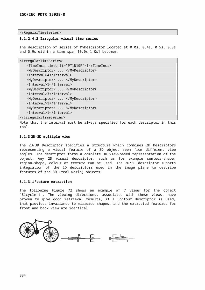
,
where i are all the successive time instants described in both descriptors (eventually pre-processed);
xi, yi zi are the successive (if available) positions of the key points;
vxi, vyi vzi the successive (if available) velocities between key points, calculated from the description as shown in the normative part;
axi, ayi azi the successive (if available) accelerations between key points;
Dti is the duration of the ith time instant;
wP, wS and wA depend on the application / query requirements (if available).
Based on this, the matching strategy can be adapted to given queries that would be expected in a specific application environment, or to take into account specific user’s interests. If the timing is important (e.g. in surveillance, looking for something at a specific time), matching can be performed only on corresponding time instants. If not, specific pre-processings can be applied on the descriptors depending on query requirements, such as time normalization. Then, different weights can be given to positions(x,y,z), speeds(x,y,z), accelerations(x,y,z) depending on the context.Rq: In most cases, for objects followed by the camera, matching as described above makes no sense in the image reference. Therefore, we recommend to discriminate the objects followed by the camera from the others prior to do any matching.
Examples of queries may then be processed as follows:
Query: In which video frames is Object k is moving to the right (or left, up, or down).Mapping #1: For all pairs of frames contained within an existence interval for object k, we compute the motion vector v(t2) = pos(t2) – pos(t1), where pos(t) are the object’s spatial coordinates at time t. We classify v as “right,” “left,” “up,” or “down” according to Figure 100.
Figure 100: Motion direction quantization used in Mapping #1Then we keep only the frames where the motion is “to the right,” and do post-processing on this set of frames to “smooth” this set of frames. We use median filtering to eliminate some of the isolated frames.
337

Mapping #2: Another means of answering the query is not to quantize v as in mapping #1, but to search as follows: the user specifies a direction vector d. We search for all frames where v.d > T, where T is a threshold. This effectively searches for motion that is within a tolerance angle about the direction of d. Again we use median filtering to reduce the number of isolated frames.
Query: Show me video frames in the last third of the video clip where Object 1 is moving to the right.
Mapping: Same as above, except we consider only time intervals that lie within the later third of the video clip.
5.5.2.3 Conditions of use
This descriptor describes the motion of a given region, i.e. it assumes that the system knows what this region is, and thus where it is located, spatially and temporally, in the visual data.
Compared to the SpatioTemporalRegionLocator or Parametric Motion, it is a simple, coarse and light description of an object motion and localization, as it is limited to one point. Typical applications may be surveillance, to check if objects pass through sensitive areas for instance, road monitoring, to check the speed of cars for instance, and object-based retrieval, motion trajectory being a key feature to discriminate between moving objects. It can also be used as an “intermediate” description to derive semantic descriptions, in context with a priori knowledge where motion trajectory has a meaning, such as in many sports.
Extraction and matching section provide example of algorithms that proved to be efficient on the MPEG-7 test set and queries used in experiments, that were designed to be as generic as possible. Therefore, in a constrained environment, these solutions can be improved/modified to better adapt to the specific application needs.
5.5.3 Parametric motion
This descriptor addresses the motion of objects in video sequences, as well as global motion. If it is associated to a region, it can be used to specify the relationship between two or more feature point motion trajectories according to the underlying motion model. The descriptor characterizes the evolution of arbitrary shaped spatial regions over time in terms of a 2D geometric transform. The spatial coordinate system of the parametric motion descriptor is fixed. It uses the default unit 'pixel' and the default local coordinate system.
5.5.3.1 Feature extraction
It is assumed that the general motion from one frame to the next can be modelled by a 2D to 2D transformation defined by a certain number of parameters. Defining an error measure as the sum of the squared intensity differences over all common pixels, i.e. the set of overlapping pixels from the two frames, the goal is to find the set of parameters that minimises the error measure. This is a regular optimisation problem where the error measure is the goal function to be minimised and the parameters of the chosen motion model are the free variables in the process.
Let’s assume that two images under consideration are I (x, y) and I’ (x’, y’). The Descriptor specifies velocities. Transformed pixel coordinates can be calculated depending on the applied motion model as follows:
Translational model: x' = a1 + xy' = a2 + y
Rotation/Scaling model: x' = a1 + a3 x +a4 y + xy' = a2 - a4 x + a3 y + y
Affine model: x' = a1 + a3 x +a4 y + xy' = a2 + a5 x +a6 y + y
Planar perspective model: x' = [(a1 + a3 x +a4 y) / (1 + a7 x +a8 y)] + xy' = [(a2 + a5 x +a6 y) / (1 + a7 x +a8 y)] + y
338

Parabolic model: x' = a1 + a3 x +a4 y +a7 xy + a9 x2 + a10 y2 + xy' = a2 + a5 x +a6 y +a8 xy + a11 x2 + a12 y2 + y
The error measure is defined as
where is the reference image and is the transformed image that is to be aligned onto the reference image. That is, the error is defined as the sum of the squared intensity differences over all common pixels.
In order to minimise the error a robust iterative method is used, which in every iteration first calculates an appropriate search direction in the parameter space, and then performs a line search in this direction. The search direction d is in all iterations calculated using the first and second partial derivatives of the error function as
Where is the identity matrix, is the gradient of the error function defined as
and is the matrix of second derivatives, namely the Hessian, defined as
The derivatives and are easily calculated from the motion models, and and
are calculated using gradient operators on the transformed image.
The epsilon is chosen as small as possible conditioned that the expression is positive definite, which implies that can be is inverted and that is a descent direction. It can be shown that such an epsilon always exists. The epsilon is found by trying to perform a Cholesky factorisation of the form . Cholesky factorisation of a matrix is only possible if the matrix is positive definite, so if the factorisation breaks down epsilon is increased and by this way epsilon can be determined.
This iterative process results in the correct motion model parameters, which are the ones that minimises the error measure and align the two frames correctly.
The goal of the minimisation process is of course to converge into a global error measure minimum, so it is important to avoid getting stuck in local minima. Therefore, optimisation has to be performed on
339

several levels of image scale. Starting with finding the correct parameter values on a coarse level, the result is used as initial parameter values on a finer scale and the minimisation is continued. Fine-tuning into the global minima, this process is performed over all scale levels and the correct global minimum is found.
To get good results and not to fall into false local minima it is necessary to have a good initial translational fit of the images before any higher-order parameters can be determined. Therefore, at each level of scale, a minimisation process updating only the translational parameters is performed before the full minimisation using all parameters of the chosen motion model is done. Experience shows that if the translational pre-step is omitted, the likelihood of falling into false minima is greatly increased. In this initial process the pure negative gradient is used as search direction and this has proven to be very robust even for frames with large disalignment.
For the quality and robustness of the algorithm it is important to maintain high precision of the image data during the processing. Therefore, in the whole process floating point precision is used for calculating and manipulation of the image data and for coarser scale calculation, high-precision gauss convolution is used. For the transform calculation, bilinear filtering is used.
When calculating the error gradient all pixels that are common in the two images contribute in the calculations, and the contribution from each pixel location is directly scaled with intensity difference of the two images, as can be seen in the formula for gradient calculation defined above. This makes the calculation sensible to outliers where the difference is large. In order to decrease this sensibility and make the algorithm more robust, initially at each scale level a histogram of the intensity differences is calculated. This histogram is used to determine a limit of the intensity difference for which pixels contribute to the gradient calculation. By omitting pixels with larger difference, outliers are removed from the gradient calculation making the process less sensible to outliers.
The complete perspective motion estimation algorithm consists of the following steps:
1. If the frames are colour images, convert them to grey-scale intensity images.2. Build a Laplacian tree of each image, that is, make a series of different scale version of each
image, going from the original image to coarser scales. This is done by convolution with a
Gaussian kernel and resampling of the image into a lower resolution.
3. Initiate the transform parameters with the resulting parameters from the previous couple of frames, or if this is the first alignment initiate them to zero.
4. Starting at the coarsest level, compute a histogram of the absolute value of differences of frames using the current transform. Compute a limit value for the differences so that 90% of pixels are below the limit and 10% of the pixels have larger absolute difference. In the following calculation use only pixels with absolute difference below the limit.
5. Initiate translational alignment iteration by setting alpha value to be a starting length for search steps.
6. Calculate the gradient of the error function regarding to the parameter values.7. Let the search direction be the normalised negative gradient.8. See if the error decreases if a step of length alpha is taken in the search direction. If it does,
update the translation parameter and loop to 6, otherwise scale down alpha.9. If alpha still is above a certain exit limit, loop to 8.10. Initiate the full alignment with all parameters by setting alpha to be a starting length for search
steps.11. Calculate the error gradient g and the second derivative matrix H of the error function regarding
parameter values, initiate epsilon to zero.12. Try to perform Cholesky factorisation of the matrix . If the factorisation breaks down, i.e. if
the factorisation is impossible to do which is the case when isn’t positive definite, then increase epsilon and loop to 12. It is guaranteed that factorisation can be done after at most
iterations.13. Let the search direction be the normalised vector , which is guaranteed to be a
descent direction.14. See if the error decreases if a step of length alpha is taken in the search direction. If it does,
update the parameters and loop to 11, otherwise scale down alpha.15. If alpha still is above a certain exit limit, loop to 14.
340

16. The resulting transformation (motion parameters) at this scale level is now calculated. Now project the result to the next finer level and loop to 4. If this was the finest level, the alignment is ready.
(see also: H. Wallin, C. Christopoulos, A. Smolic, Y. Abdeljaoued and T. Ebrahimi,"Robust Mosaic construction algorithm", ISO/IEC JTC1/SC29/WG11 M5698, Noordwijkerhout, Netherlands, March 2000)
5.5.3.2 Similarity matching
5.5.3.2.1 Velocity-based similarity measures
The principle of the velocity-based similarity measure relies on the generation of the velocity fields associated with the motion models, followed by subsequent comparisons between these 2D velocity vectors.
Let M1 and M2 be the two motion models (which may be translational, rotation/scaling, affine, projective or quadratic) associated with object regions R1 and R2, respectively. Both objects are assumed to be matched so that their gravity centers coincide. A distance d(M1, M2) between the two models is defined as follows:
d(M1, M2) ,
where V1(i) and V2(i) denote the velocity vectors at point i, associated with models M1 and M2, respectively and denotes a distance between 2D velocity vectors.
In order to reduce the computational complexity of the above-described similarity measure, a simplified version is derived. The principle consists of no longer considering the whole regions R1 and R2, but only small rectangular windows representative of the overall motions. From a practical point of view, these windows can be centered at the gravity center of each moving object and have the same size. In this case, the simplified velocity-based similarity measure within the window W, denoted by Dis expressed as follows:
This technique provides a generic strategy for comparing object motions of different model types (e.g. comparison between a motion described as an affine model and a motion described as a quadratic or projective model). It is also possible to compare a motion specified by a model with motion exclusively known by its dense velocity field extracted by using an optical flow algorithm.
As distance measurements between 2D velocity vectors, we recommend to use the following functions:
L1 norm: = V i V i1 2 1( ) ( ) = V i V i V i V ix x y y1 2 1 2( ) ( ) ( ) ( ) ,
L2 norm: = V i V i1 2 2( ) ( ) = V i V i V i V ix x y y1 2
21 2
2( ) ( ) ( ) ( ) ,
Correlation function: = 1.0 - V V
V V1 2
1 2 2 2
, ,
Amplitude absolute difference function: = V i V i1 2( ) ( ) .The above-mentioned functions suit different kinds of queries, from low-level queries where certain dense flow fields are searched, to high level queries, such as "search for objects approaching the camera", or for "objects describing a rotational motion". The end-user will select the appropriate function. For example, when searching collinear flow fields of a specific type, the correlation function is recommended. In a query by example scenario, where accurate matching is required, we recommend the use of L1 or L2 norm.
341

5.5.3.2.2 Parameter-based similarity measure
A second way to define a similarity measure for motion-based retrieval consists of directly considering the parameter space. The parameters of the parametric object motion descriptor themselves carry distinctive and compact motion information associated with certain kinds of motion like translation or scale. Therefore it is possible to define a distance measure for comparison of two motions in the context of search and retrieval applications, that directly compares the descriptor values.
Given two sets of parametric object motion parameters a = (a1, a2, ..., aN)T and b = (b1, b2, ..., bN)T, where N is the number of parameters of the applied motion model, the distance measure d is defined as follows:
The weighting factors wn allow the individual adjustment of the sensitivity of the distance measure for each motion parameter. For instance if we set w1 = w2 = 1 and wn = 0 for n > 2, the distance measure relies only on the translation parameters without taking the other parameters into account. In addition to query-by-example, this enables the formulation of higher order queries targeting on certain kinds of motion, e.g. "find all translations to the right" or "find all zooming-in motions, regardless of translation". By default the translational parameters should be normalized to the image dimensions to make the distance measure independent of the spatial sampling grid and to adjust the numerical range of translation and higher order parameters.
The planar perspective and the parabolic model are very well suited for mosaicing applications, where highest possible accuracy and stability is required for the motion description over a long period. However, the higher order parameters are physically not very meaningful and we recommend not using them for matching applications. Of course a higher order description can always be converted to (approximated by) a motion model of lower order. This is also necessary if the two motion parameter sets to be compared do not use the same motion model.
The main strong points of this technique are the very low computational complexity (weighted sum of a few numbers) and the direct possibility to derive mid-level queries on certain kinds of motion. If the spatial reference of the transformation coincides with the centroid of the considered video object, the translation parameters directly express image translation. Similar expressions can be derived for zoom or rotation. This makes it possible to use query-by-specification to search directly for certain kinds of motion like “find all right translations, ordered by speed” or “find all fast up-scales”.
5.5.4 Motion activity
A human watching a video or animation sequence perceives it as being a slow sequence, fast paced sequence, action sequence etc. The activity descriptor captures this intuitive notion of ‘intensity of action’ or ‘pace of action’ in a video segment. Examples of high ‘activity’ include scenes such as ‘goal scoring in a soccer match’, ‘scoring in a basketball game’, ‘a high speed car chase’ etc… On the other hand scenes such as ‘news reader shot’, ‘an interview scene’, ‘a still shot’ etc. are perceived as low action shots. Video content in general spans the gamut from high to low activity, therefore we need a descriptor that enables us to accurately express the activity of a given video sequence/shot and comprehensively covers the aforementioned gamut. The activity descriptor can be used in diverse applications such as content re-purposing, surveillance, fast browsing, video abstracting, video editing, content based querying etc.
5.5.4.1 Feature extraction
The extraction of the descriptor values is based on 16x16 macroblock motion vector values. We assume that the shot segmentation has been done so that we can describe the extraction in two stages, first for a frame and then for the entire shot. In our experiments we extracted the motion vectors from the compressed MPEG-1 content that constitutes the MPEG-7 test-set. With uncompressed content, we can carry out block matching based motion estimation to get the motion vectors. This extraction procedure works best in the compressed domain with video of MPEG-1 quality or higher because the search radius is then assured to be large enough to capture the motion
342

completely. For low bit rates, lower search radii might be used and hence the motion vectors may give misleading results. In that case, full decompression followed by block matching on the uncompressed content would be the only solution.
5.5.4.1.1 Intensity characteristics
We consider only P frames/objects and for Intra-coded blocks the motion vector magnitude is considered to be zero. The parameters for a frame consist of the average motion vector magnitude
and the standard deviation of the motion vector magnitude and as defined in the normative part.
5.5.4.1.2 Directional characteristics
For each object or frame the “angle matrix" A is defined as:
where (xi,j,yi,j) is the motion vector associated with the (i,j)th block.
We consider only P frames/objects, and construct the descriptor for a frame in the following steps.
1. For Intra-coded blocks, Ang(i,j) =0.2. The average angle per macro-block of the frame/object Aavg is given by:
3. Compute the variance of as follows:
The Motion Vector Based Parameters for a shotWe find the parameters for a shot using one of the following methods:
a. Compute the descriptors of all the P frames in the shot. Get the average motion vector magnitude per macro-block on motion vectors for the entire shot. Use the frame with Cavg
closest to this average.b. Find the average of all the parameters over the shot. Use the set of averages as the feature
vector for the shots. In addition to the average of the shot parameters, we can also calculate the variance (or standard deviation) of the average and deviation parameters, as well as of the other parameters. The deviation parameters provide confidence measures for the average based descriptor parameters described earlier. Thus we have four statistical parameters and three run-length features extracted using motion vector magnitudes and four statistical parameters extracted using the direction of the motion vectors.
343

c. Find the Cavg for each P frame in the shot. Find the median of the Cavg over all the P-frames and let the frame number of the median be n. Then use the descriptor of frame n as the shot descriptor.
d. Choose a P-frame at random from the shot and use its descriptor as the shot descriptor.Method b is our method of choice for the calculation of the shot descriptor parameters based on motion vectors.
Quantization of each value:
The Intensity parameter is obtained by uniformly quantizing the square root of the variance, i.e. the standard deviation, computed above to fit on a scale of 1-5. For MPEG-1 motion vectors, the following pseudo-code (f_var is the variance) illustrates the quantization procedure:
if (f_var <3.9) intensity=1;
else if (f_var < 10.7) intensity=2
else if (f_var < 17.1) intensity=3;
else if (f_var < 32) intensity=4;
else if (f_var >=32) intensity=5;The spatial attributes are obtained by quantizing the run-length features Nsr, Nmr and Nlr to 6, 5 and 5 bit integers respectively. The DominantDirection is obtained by quantizing the average angle Aavg to a 3 bit integer, which covers the following values: 0, 45, 90, 135, 180, 225, 270, 315.
5.5.4.1.3 Temporal characteristics: Shot activity histogram
The Shot activity histogram consisting of 5 bins corresponding to 5 levels of activity can be derived using the activity levels of the individual frames in the shot. If the intensity of activity is expressed on a finer scale than 1-5, uniform quantization is used to map it to a scale of 1-5. The histogram is then derived using the quantized activity levels of the individual frames.
5.5.4.1.4 Spatial localization characteristics
The instances of the spatial localized motion activity are given as the statistics that are calculated based on “(3D) division blocks” in a shot shown as Figure 101. One division block consists of 2D blocks that are placed at the same position on every frame within the shot. Each 2D block contains some macro-blocks for coding, therefore each 2D block has the corresponding several motion vectors. The spatial localized motion activity is calculated based on the motion vectors’ magnitudes on only P frames/objects. The procedures of spatial localized motion activity extraction are described in the following.
344

Figure 101 Extraction of spatial localized motion activity in a shot
5.5.4.1.4.1 Division block arrangements
Division block arrangements are explained as follows. The number of division blocks for a shot is 4, 16, 64, or 256. The corresponding four styles of division block are shown in Figure 102.
Figure 102 Division block arrangementsThe 3D blocks painted are the examples of the division blocks. Those division blocks are constructed based on the coding macro-blocks. (In Figure 102, the smallest blocks drawn on the first frames denote such macro-blocks.)
For the explanation below, the 3D division blocks are denoted by where m and n are coordinates. The consists of 2D blocks denoted by where f denotes the frame number.
The resolution of division block is decided for the requirements of applications that use the above activities. 4 (2x2) division is suitable for simply categorization, at very small amount of storage. 64(8x8) or 256(16x16) division is useful for more complex situation, such as strict query retrieval.
5.5.4.1.4.2 Spatial localized activity calculations
For a shot the activity matrix R is defined as:
where
345

where (xfij, yfij) is the motion vector associated with the (i, j)th coding macro-block in the frame f. (In here the activity matrix is defined for a shot/object, i.e. 3D matrix.) The rfij denotes the motion vector’s magnitude.
The spatial localized activity for a shot is calculated by the following steps.
Step 1. (Activity calculation based on the magnitudes of the motion vectors)
The average of motion vectors’ magnitude per each division block is given by;
where the coding macro-blocks fij (at the coordinates (i, j)th in the frame f) are on only P frames and only Inter-coded or Skipped macro-blocks. For Skipped macro-blocks, rfij=0. The denotes the
number of such Inter-coded/Skipped macro-blocks in the division block . Since the amn is the average value per motion vectors, the differences of the sizes of division blocks in a certain resolution are canceled. If is equal to 0, amn is set to 0 and continue to the following step.
Step 2. (Normalization procedure by calculating the percentage distribution)
Calculate the percentage distribution for a shot as follows;
where .
The are regarded as the spatial localized motion activity. If SA is equal to 0, that is the case in Step 3.
Step 3. (Exception Procedure for the case that the division block has no information of motion)
If all of the macro-blocks in the division block is Intra-coded macro-block, the above calculations in Step 1 and Step 2 are impossible. If all of the motion vectors in the division block are equal to 0, the above calculation in Step 2 is impossible. At that situation, the spatial localized motion activity is given by the average distribution per the number of division blocks in the resolution:
where ND is the number of division blocks (i.e. 4, 16, 64, or 256). This distribution expresses the information that the shot has no motional tendency.
5.5.4.1.4.3 Quantization
The spatial localized activities are linearly quantized into 8 levels (3 bits). The quantization procedure is given as
where
.
346

L is the number of levels of quantization, i.e. L=8 (3bits). is the quantized spatial localized activity. Q denotes a step size of quantization. Since the expresses the probability values dependent on the resolution of the division block, the step size Q is given by the above constant formula. ND denotes the number of division blocks on the resolution.
5.5.4.2 Similarity matching
We have used two different search procedures. We use a subset of the parameters to illustrate our search procedure.
The first procedure is as follows. Let the query shot be Sa and the test shot be S, then the “distance” D(S,Sa) between S and Sa is computed as follows:
In case there is a division by zero for one term in the sum, this term is not calculated and set to zero.
The second procedure is a “cascaded” search in which we use one descriptor feature at a time and successively refine the search with the other features. The cascaded procedure is slower but sometimes gives slightly higher accuracy.
Note that for the SpatialDistribution term, if the frame height h of a VideoSegment A is k times the frame height of a VideoSegment B, then the spatial parameters of VideoSegment B need to be multiplied by k before comparison with the spatial parameters of VideoSegment A.
5.5.4.2.1 Spatial localization characteristics
In the following, procedures for (directional motion tendency based) shot categorization and for similarity retrieval by using spatial localized activity are shown.
5.5.4.2.1.1 Shot categorization
Shots are categorized into 10 classes with regard to the directional tendency of the intense motion appearance; (1) Top, (2) Bottom, (3) Left, (4) Right, (5) Top-Left, (6) Top-Right, (7) Bottom-Left, (8) Bottom-Right, (9) Center, and (10) None, i.e. no directional tendency. To examine the directional tendency, the following nine weighted-masks are introduced for calculating the product-sums between the mask weights and spatial localized activities.
The weight/coefficient of the mask at the coordinates (m, n): wmn is given by:
where .
dmn is the normalized distance between the point of coordinates (m, n) and the ‘key-point’ of the mask which is drawn in Figure 103. Point ‘Top-Left’ is the key-point for making the weighted-mask for detecting the top-left directional tendency of motion, and it is similar about the other eight key-points. The dmn is normalized by the size of the division block. is a constant for adjusting the spread of the weights/coefficients; currently =4.0.
347

Figure 103 Key-points for the weight masksThe product-sums SKP (KP expresses each key point) between the spatial localized activities of the target shot and the mask weights of the above nine masks are calculated by;
,
and the nine values {STop, SBottom, SLeft, SRight, STop-Left, STop-Right, SBottom-Left, SBottom-Right, SCenter} are derived.
The directional tendency of the target shot is decided by detecting a maximum of the above nine values; denote it by SMAX. Furthermore, the following exception processes (EP) are added.
EP 1. (Detection of shot that has no direction tendency)
Detect a minimum of the above nine values; denote it by SMIN. The ratio SMIN/SMAX is greater than a threshold Tvar, the target shot is judged into the category: (10) None. Currently Tvar=0.85.
EP 2. (Detection of whole frame-based motion tendency)
For example, consider the case that STop-Left is truly a maximum and SLeft is close to the maximum. In that case an observer feels that the target shot has the whole frame-based motion tendency to the left. This exception process deals with such situation.
If the maximum is STop-Left, STop-Right, SBottom-Left, or SBottom-Right, detect a secondary maximum of the above nine values; denote it by SSMAX. The ratio SSMAX/SMAX is greater than a threshold Tcrnr, the target shot is judged into the corresponding category shown in the following Table 21. Currently Tcrnr=0.75.
Table 21: Classified categorySMAX SSMAX Classified
category
STop-Left STop or STop-Right (1) Top
SLeft or SBottom-Left (3) Left
STop-Right STop or STop-Left(1) Top
SRight or SBottom-Right(4) Right
SBottom-Left SBottom or SBottom-Right (2) Bottom
SLeft or STop-Left (3) Left
SBottom-Right SBottom or SBottom-Left (2) Bottom
SRight or STop-Right (4) Right
348

Note: The simple method of judging the directional tendency of motion is the comparison between the activities of some independent directional blocks that was divided in advance. The reason whereby such above weighted-masks, which spread over the whole frame, are used is that the directional tendency of motion depends on the whole distribution as well as the local distribution. Of course, the method of categorization based on the spatial localized activity is not restricted to the above one.
5.5.4.2.1.2 Similarity retrieval
Similarity retrieval is realized by calculating the distance between the spatial localized activities of the query and that of the target shot as:
.
A target shot T that has the minimum DQ(T) is decided as the most similar shot to the query Q.
Note: Of course, the method of similarity retrieval based on the spatial localized activity is not restricted to the above one.
5.5.4.2.2 Conditions of usage
The main motivation for the motion activity descriptor is provided by the interactive video browsing application, hence the emphasis is more on simple classification of video shots and less on accurate classification. The extraction is fast with compressed content since it relies on motion vectors, which are readily available in the compressed domain. The extraction is much slower with uncompressed content, but note that it is still simpler than any other motion based extraction. Furthermore, since the descriptor captures gross characteristics, it can be successfully used with low resolution motion estimation such as the block matching used by MPEG-1/2 compressors, thus obviating the need for more computationally intensive techniques such as optical-flow based motion analysis etc. The extraction needs to be normalized with respect to the content parameters, but is otherwise unaffected by changes in encoder/content parameters such as bit rate, frame rate, frame resolution etc. The descriptor works best with high quality content but is fairly robust to degradation in quality, in other words, it works well for both high and low bit rate video.
Note that the coarseness of the descriptor prevents it from being a high-accuracy descriptor for content-based querying of large databases. It is thus most successful in intra-program browsing applications, and moderately successful in inter-program browsing applications. Inter and intra-program browsing works best when the intensity, spatial, temporal and direction attributes of the descriptor are combined. The intensity parameter is the key attribute while the other attributes help refine the results got by using the intensity parameter alone. The descriptor is also successful in “pre-filtering” or pruning the search space down to a size that allows use of more computationally intensive descriptors to get more accurate matches. It is also useful in general as a simple first line of attack in any kind of content analysis and description.
While the descriptor is at first glance a descriptor for a video segment, note that it can also be used to describe a collection/concatenation of video segments. Calculation of the temporal attribute of a concatenation of shots is the most straightforward but calculation of the other attributes is certainly feasible and meaningful. Hence, while the descriptor of a 1 second video segment can be easily calculated and used, the motion activity descriptor of even an hour long segment is still meaningful and useful.
5.6 Localization tools
5.6.1 Region locator
The RegionLocator enables the localization of regions within images or frames by specifying them with a brief and scalable representation of a Box or a Polygon. The determination procedure consists of the following two steps.
349

1.Extraction of vertices of the region to be localized.2.Localization of the region within the image or frame.
5.6.1.1 Extraction
Figure 104: Overall descriptor estimation process for 2-D visual objects.
A block diagram of the overall extraction of a RegionLocator is shown in Figure 104. The steps involved are (1) segmentation of an image into objects, (2) extraction of the bitmap of object of interest, (3) estimation of a closed, approximating contour of the object and finally (4) encoding of the polygon vertices of the contour. The segmentation map consists of segmentation labels at each pixel, each label corresponds to a distinct visual object. Then, a binary map is created, with values "valid" (true, 1, or 255) wherever segmentation label equals the objectID of interest, and "invalid" (false, or 0) elsewhere. The segmentation process is outside the scope of the extraction. The closed contour approximation procedure gets, as input, the bitmap indicating the validity of each pixel.
The process of contour approximation consists of the following two steps:
1. Extract the border pixels of the region of interest. This can be realized in the case of a single compact object by line scanning the binary object map starting at a boarder of the map until an object pixel is detected and then following the contour of the object in one direction e.g. clockwise.
2. Contour approximation: deletion of vertices of the contour which are below a threshold according to a cost function.
acceptable precision. Starting from a very detailed contour representation those vertices which only cause a small error in the contour approximation can subsequently be removed. For this purpose an applied cost function can for instance be an approximation of the region area being removed by deleting a vertex. So in a first step the algorithm calculates the area error for each vertex based on the triangle which is built by the vertex considered and its neighbors. If a vertex is removed based on the low cost, the area error of the removed vertex is added to the new area errors computed for the neighbor vertices. Accordingly successive removing the smallest vertex until the cost of the removal is higher than a threshold results in an approximation of the contour.
This automatic process can also be replaced by a manual input of important vertices of the contour.
5.6.1.2 Localization
In principle the RegionLocator is used as hyperlink between the description and the described media. So this link can be followed in two directions: from the description visualizing the described region in an image or from the image identifying the part of the description related to a certain area in the image. In both cases decoding the RegionLocater again to a bitmap of the region can be used for visualization and interaction.
The rendering can be processed in two steps: first decoding the list of vertices and inserting the contour into the bitmap. Then executing a line scan and inserting the points inside the contour into the bitmap. Which pixels of the line processed are inside the contour is determined by counting the contour crossings of the line: after an odd number of contour crossings of the line the pixels on this line belongs to the contour, after an even number of crossings they do not.
350

5.6.2 Spatio-temporal locator
The SpatioTemporalLocator describes spatio-temporal regions in a video sequence and provides localization functionality especially for hypermedia applications. It consists of FigureTrajectory and ParameterTrajectory. Moving regions in multiple frames are described by one or several sets of a reference region and its motion. FigureTrajectory and ParameterTrajectory describe each set of a reference region and a motion. The two description schemes are selected according to moving object conditions. In general, if a moving object region is rigid and the motion model is known, ParameterTrajectory is preferable due to its compactness. On the other hand, if a moving region is non-rigid, FigureTrajectory with a polygon is suitable. FigureTrajectory is also suitable for a rigid region moving with complex motion, where the motion model is not known.
Figure 105: SpatioTemporalRegion
5.6.2.1 Figure trajectory
FigureTrajectory describes a spatio-temporal region by trajectories of the representative points of a reference region. Reference regions are represented by three kinds of figures: rectangles, ellipses and polygons. For rectangles and polygons, the representative points are their vertices. Although there are four vertices for a rectangle, only three of the four are described because the rest can be easily calculated. For ellipses, three vertices of their circumscribing rectangles are selected as the representative points.The trajectories are interpolated using the TemporalInterpolation The reference region description in SpatioTemporalLocator is omitted because the TemporalInterpolation can directly indicate the representative points of figures.
Figure 106: Motion Descriptions for FigureTrajectory
5.6.2.1.1 Inside/Outside determination
The determination procedure consists of the following two steps.
1.Extraction of vertices at the given time.2.Determination if the given point is inside or outside the figure represented by the vertices.
Step 1 is simply processed by extracting the coordinate from the Temporal Interpolation. This procedure is explained in the TemporalInterpolation section of this document. The procedure for Step 2 depends on the type.
Polygon
Let V1, V2 ...Vn denote vertices. A point Q is check if it is inside or outside the polygon. If there exists an index i in {1,...,n} such that Q = Vi, then Q is inside, otherwise
351

define W as a summation of angles in radian defined by two vertices and
Q: W =rad(V1- Q,V2- Q)+ ....+rad(Vi- Q,Vi+1- Q)+....+rad(Vn- Q,V1- Q) , where (for two non-zero vectors a, b in R2)
, .
If a point Q is inside the polygon, W is equal to -2 . Otherwise, W is equal to 0.
Figure 107: Vectors from a check point Q to vertices
Rectangle
Let V1, V2 and V3 denote the vertices described by the Temporal Interpolation. Then, the remaining vertex V4 is calculated by V4 = V1 - V2 + V3.
For inside/outside determination, we use the same algorithm as for polygon.
Ellipse
The center of the ellipse C0 and the lengths of the two axes a, b are given by
Using these equations, the eccentricity of the ellipse e is calculated by
Also, the two focuses F1 and F2 are given by
respectively. Then, a point Q is inside the ellipse if and only if
is satisfied.
352

5.6.2.1.2 Feature extraction
Figure 108 shows the feature extraction procedure for the FigureTrajectory. At first, binary representation mask images are input. Then, polygon vertices are generated by approximating the masks by polygons. Correspondences between vertices of polygons in two consecutive frames are determined at the correspondence determination process. Finally, the correspondence determined vertices are input to the TemporalInterpolation D encoder and described by the D. The feature extraction method of the TemporalInterpolation D is explained in [3].
Figure 108: Feature Extraction Process for the FigureTrajectory.
Let us denote the contour of the segmentation mask by , where CN is
the number of pixels on the contour. Vertices of an approximated polygon are denoted by ,
where denotes the number of the vertices. Also let denote the target number of vertices. For each , the approximation error , which is caused by removing the vertex , is defined as the area of the triangle
having the vertices, , , and (Figure 110: left). The vector is defined as
,
and used to reduce the approximation error (Figure 110: right). The following is the algorithm for polygon approximation.
Figure 109: An The contour is set to the initial polygon.
353

Figure 110: The approximation error and the vector used to reduce the error.
Polygon Approximation Algorithm
1. Set for and .
2. If , terminate.
3. Find which minimizes .
4. Set and .
5. Set , , …, and . Go to Step 2.
Let , and denote the vertices of the polygon at , the gravity center of the polygon at and the Euclidean distance between two points and , respectively. Then, the algorithm to determine correspondences between polygon vertices is as follows.
Correspondence Determination Algorithm1. Calculate , , and .
2. Find , which minimizes
.
3. Determine that moved to .
354

Figure 111: An example of possible correspondence combinations.
5.6.2.2 Parameter trajectory
ParameterTrajectory describes a spatio-temporal region by a reference region and trajectories of motion parameters. Reference regions are described using the Region Locator. Motion parameters and parametric motion model specify a mapping from the reference region to a region of an arbitrary frame. The trajectories of the motion parameters are interpolated and described using the Temporal Interpolation.
Figure 112: Motion Descriptions for ParameterTrajectory
5.6.2.2.1 Inside/Outside determination
The determination procedure consists of the following three steps.
1. Extraction of motion parameters at the given time.2. Calculation of vertex coordinates.3. Determination of whether a given point is inside or outside the figure represented by the
vertices.Step 1 is simply executed by extracting the coordinates at a given time from the TemporalInterpolation. For Step 2, the vertices of the box or the polygon are transformed by the extracted motion parameters. If the RegionLocatgor represents a box and the ellipseFlag is true (DDL representation) or ‘1’ (binary representation), the transformed vertices are treated as the vertices of the circumscribing rectangle of an ellipse. The procedure for Step 3 is exactly the same as in the case of the FigureTrajectory for rectangles, ellipses and polygons.
355

5.6.2.2.2 Feature extraction
Error: Reference source not foundFigure 113 shows the feature extraction procedure for the ParameterTrajectory. In this case too, the input of the process is binary representation mask images. The procedure is for the most part the same as that for the FigureTrajectory. The difference is the motion parameter estimation process inserted between the correspondence determination and the TemporalInterpolation D encoder. It estimates motion parameters of a given motion model using displacement vectors between the vertices in the current frame and the reference frame. In the reference software, the vertices of the first frame are stored in the reference buffer as the reference.
Figure 113: The Feature Extraction Process for the ParameterTrajectory.
The motion parameter estimation between a reference frame and another frame is easily accomplished by using the least square method. In the following, it is assumed that the number of motion parameters is equal to or greater than the number of displacement vectors .
Let and be the i-th vertex position in a reference frame and the displacement vector of the i-th vertex, respectively. The displacement vector is derived as the difference vector between the corresponding vertices in the two frames, where and is the time of the current and the reference frame. Also, denote the estimated position of the i-th vertex by
. and are expressed by , and motion parameters. For example,
and for affine transformation model.
Motion parameters are estimated by solving the simultaneous equations
where the estimation errors are defined as .
5.6.2.3 Conditions of usage
Selection of FigureTrajectory and ParameterTrajectoryThe FigureTrajectory and the ParameterTrajectory are selected according to moving object conditions. If a moving object region is rigid and the motion model is known, ParameterTrajectory is preferable due to its compactness. On the other hand, if a moving object region is non-rigid, FigureTrajectory with a polygon is suitable. FigureTrajecyoty is also suitable for a rigid region moving with complex motion, where the motion model is not known.
Intervals between key points
356

If the interval lengths between key points are very short, the SpatioTemporalLocator is no longer efficient. In case that first order polynomials are used for interpolation functions, the average interval length should be over 1 frame so that the SpatioTemporalLocator is efficient. In case that second order polynomials are used, the average should be over 2 frames.
5.7 Other visual tools
5.7.1 Face recognition
The face recognition descriptor represents the projection of a face vector onto a set of 48 eigenvectors which span the space of all possible face vectors. These eigenvectors are comonly called eigenfaces.
5.7.1.1 Feature extraction
The FaceRecognition feature set is extracted from a normalized face image. This normalized face image is obtained by scaling of the original image to 56 lines with 46 luminance values in each line. The centre of the two eyes in each face image should be located on the 24th row and the 16th and 31st column for the right and left eye respectively. This normalized image is then used to extract the one dimensional face vector which consists of the luminance values from the normalized face image arranged into a one dimensional vector using a columnwise raster scan starting at the top-left corner of the image and finishing at the bottom-right corner of the image.
The FaceRecognition feature set is then calculated by projecting the one dimensional face vector onto the space defined by the basis matrix which is defined in Annex A.1 of the FDIS.The features are given by the vector where and is the mean face vector defined Annex A.2 of the FDIS.
The features are normalized and clipped using the equation
where Z=16384 is the normalization constant. Then all the features are re-quantized linearly as follows:
The feature set is then stored as 5-bit integers.
5.7.1.1.1 Automatic face image localization
There are four steps in this algorithm, as shown in Figure 114. The Color Segmentation algorithm is used to segment the input image into candidate regions by skin color. Then the Facial Feature Extraction algorithm is used to extract facial feature points in the candidate regions such as eyes, eyebrows etc.. The Face Candidate Detection algorithm is then used to detect all of the possible faces in the input image. By this stage all of the possible faces should have been detected, however, there may be non-face regions which have been detected as faces, and there may be more than one candidate face for one actual face. These first three step form the Coarse Detection part of the algorithm. Fine detection is performed in the Face Confirmation stage which is used is to discard falsely detected non-face regions and eliminate multiple candidate faces for each true face.
357

Color Segmentation
Face FeatureExtraction
Face CandidateDetection
FaceConfirmation
Coarse Detection
Figure 114: Block Diagram of the Automatic face Image Localization Algorithm
5.7.1.1.1.1 Color segmentation
Skin color is an important feature of human faces. The possible face regions can be obtained by color segmentation. In color image processing, color is usually represented by three components. According to specific conditions in applications and the performance required, some examples of these three components include: RGB, rgb (normalized RGB), YCbCr, YIQ, HSI, HSV, YUV . Each of these representations behave differently when used for skin color segmentation.
Since the main purpose of color segmentation in our algorithm is to find possible face regions, the accuracy required for this part of the algorithm can be quite low. The components YCbCr, where Y is the intensity component while Cb and Cr are chrominance components, are used since they are widely used in the MPEG and JPEG standards
In the Cb-Cr plane, human skin forms a relatively tight cluster, which can be modeled as Gaussian distribution as shown in Figure 115 a). White pixels in the figure represent skin colors. The horizontal axis is Cr and the vertical one Cb. Based on this skin color distribution, we can obtain the candidate skin color regions in an image.
a) b) c)
Figure 115: A color segmentation example, a) the skin color region in the Cb-Cr plane b) original image c) results of the color segmentation algorithm
In some images the illumination is varying, so that the complexion is out of the range of normal skin color. As a complementary part of this algorithm, the area of candidate regions after color segmentation is calculated. If this area is smaller than a threshold (the area of the smallest face), the input image is regarded as a pseudo-gray image, and the candidate regions are modified to include the whole image.
5.7.1.1.1.2 Facial feature extraction
It is reasonable to assume that the in-plane rotation of a face image will be such that the two eyes are both higher than the mouth in the image. Under this constraint, facial features, such as eyebrows, eyes and the mouth, can be detected by extracting horizontal texture. The facial features extracted this way are referred to as objects of horizontal texture. These objects of horizontal texture are extracted from a low resolution version of the input image using Gaussian derivate filters. The resulting image is called an image of facial features (IFF).
To reduce the effect of varying illumination, size, pose and facial expression on the presentation of facial features, two models, six scales and three thresholds are used to extract the feature points. The
358

two models used are mosaic and line-mosaic as shown in Figure 116. For each of the two models, five scales are selected, which are 2x2, 3x3, 4x4, 5x5, 6x6 and 2x2, 3x2, 4x2, 5x2, 6x2 respectively (see Figure 116).
2x2 3x2 4x2 5x2 6x2
2x2 3x3 4x4 5x5 6x6
Figure 116: Mosaic and Line-Mosaic modelsThe algorithm synthesizes (using the binary OR operator) the IFFs at all resolutions to generate the IFFs for different models and thresholds. A block dioagram of this procedure is shown in Figure 117. Figure 118 shows a set of IFFs of the gray-level image corresponding to the image in Figure 115 b). Facial features which are too large or too long are discarded by applying a prior knowledge. The facial features in each IFF are then labeled and their gravity centers and other geometrical parameters are recorded in a one-dimension array. Each facial feature is represented by its gravity center so it may be referred to as a feature point.
Line-mosaic
Scale 1
Scale 2
Scale 3
Scale 4
Scale 5
Featureextract th1
ORFeature
extract th2
Featureextract th2
IFF4 TH1
Mosaic
Scale 1
Scale 2
Scale 3
Scale 4
Scale 5
Featureextract th1
Featureextract th2
Featureextract th3
OR
IFF1 TH1
InputImage
IFF5 TH2
IFF6 TH3
IFF2 TH2
IFF3 TH3
359

Figure 117: Block diagram for the facial feature extraction algorithm
Figure 118: IFFs generated by various models and thresholds
5.7.1.1.1.3 Face candidate detection
Face candidate detection is carried out using the arrays mentioned above. The algorithm models the human face with a group of three facial features that have a triangular spatial relationship which corresponds to the unique spatial relationship of the two eyes and the mouth. The detection of this triangular spatial relationship is divided into two stages: a) finding groups of two eyes and b) generating face candidates by finding corresponding mouths in regions determined by the two eyes. The first stage involves finding groups of eyebrows and eyes, referred to as eye-pairs. A face candidate is declared when a corresponding mouth that meets certain requirements is found.
5.7.1.1.1.3.1 Finding eye-pairs
The possible forms of an eye-pair allowed in the algorithm are shown in Figure 119. Eyebrows can be missed while eyes can’t. This is ensured by robust facial feature extraction. The angle between the line connecting eyes and the horizontal line is set to range within [-,+] where = . The constraint on this angle can be altered easily by adjusting parameter .
+ +- -
a
+ +-
b
+ +-
c+ +
d
Figure 119: Possible forms of an eye-pair. ‘-’ represents the eyebrow and ‘+’ represents the eye.
To find a possible eye-pair, two directional triangular regions, P^(,h) and P<(,h), are defined and shown in Figure 120 (a) and (b) respectively. P^(,h) represents the region in which the algorithm seeks the corresponding eye given an eyebrow. P<(,h) represents the region in which the algorithm seeks the corresponding right eyebrow and right eye given the left eye. Noting the influence caused by glasses and hairs, another directional triangular region P<(,h1,h2), is defined and shown in Figure 120 (c). The algorithm allows a noise point in the white region.
360

Figure 120: Defined regions.Definition 1:P^(,h) is defined as the region enclosed by isosceles triangle ΔPLR where h denotes the
height, LR is horizontal, PL=PR and LPR=2.Definition 2:P<(,h) is defined as the region enclosed by isosceles triangle ΔPTB where h denotes the
height, TB is vertical, PT=PB and BPT=2.Definition 3:P<(, h1, h2) is defined as the shaded region in isosceles triangle ΔPTB where h1 and h2
denotes the heights of ΔPUV and ΔPTB respectively, h2>h1, PT=PB, UV and TB are vertical and BPT=2.
All parameters of the defined regions are set in advance but can be modified. The procedure for finding eye-pairs in IFFs is as follows:
(1) Regard the present feature point as a left eyebrow PLB and seek the corresponding left eye PLE in region PLB^(,h). If there is no left eye found in that region, the present feature PLB is regarded as the left eye PLE and no left eyebrow is declared.
(2) Given the left eye PLE, seek the corresponding right eyebrow PRB in region PLE<(,h1,h2). When there is a left eyebrow declared in (1), the parameters of PLE<(,h1,h2) can be modified with the spatial relationship of PLE and PLB. To avoid missing small faces, the search is repeated once more in the region PLE<(,h). If there is no right eyebrow sought, no eye-pair is declared, then the next feature in the one-dimension array is regarded as the present one, and go to (1).
(3) Given the right eyebrow PRB, seek the corresponding right eye PRE in region PRB^(,h) where the parameters, and h, can be modified with the spatial relationship of PLE and PRB . Declare an eye-pair in which PLE and PRB are regarded as the left and right eyes respectively. And if there is a right eye sought, declare another eye-pair that regards PLE and PRE as the left and right eyes respectively. Regard the next point in the array as the present feature and go to (1)
(4) Merge eye-pairs with the same left and right eyes. Analyze geometrical parameters of all features in an eye-pair to see if certain requirements are met. If not, discard the eye-pair.
5.7.1.1.1.3.2 Generating face candidates
After an eye-pair is determined, the algorithm seeks possible mouths in a rectangular region, in which the two eyes are regarded as its two upper vertices. It analyzes each mouth sought with the deformable template shown in Figure 121 to generate a face candidate. and in Figure 121 respectively represent the left and right eye in the template. The width W= , height H and obliquity of the deformable template are adjusted to fit and on the PLE and PRE in the eye-pair respectively and to make the bottom of template go through the mouth point . If the following requirements are met, a face candidate is declared.
(1) D<W where D denotes the long diameter of facial feature whose gravity center is ;(2) HÎ[k1W, k2W] where k1 and k2 are both constant coefficients.(3) N11, N22, N3=N4=N5=0 where the number of feature points in the sub-regions (1,2,3,4,5) of the
template is N1, N2, N3, N4 and N5 respectively.
361
(a) (b) (c)
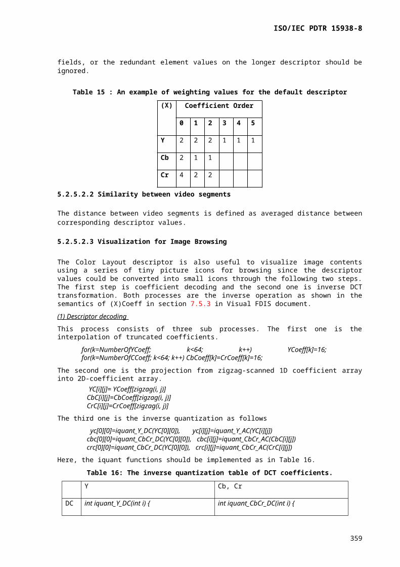
When a face candidate is declared, the algorithm keeps a record of the gravity centers and other geometrical parameters of all facial features involved. The template used to generate the candidate is referred to as the detection template of that specific face candidate. To compensate for the influence of glasses and hair, the algorithm allows one feature point in sub-region 1 and two feature points in sub-region 2, the nostril sub-region.
PLe PRe
1
3
24 5
W
H
Figure 121: Face candidate detection template
5.7.1.1.1.4 The face confirmation algorithm
Once a face candidate has been detected, the image region containing the candidate face is extracted from the luminance component of the original image. This region of the original image is then scaled and rotated to form a face candidate image that contains 48 lines with 36 luminance values in each line. The center of the two eyes in each face candidate image is located on the 20 th row and the 11th
and 26th column for the right and left eye respectively.
The face extraction algorithm must be able to extract faces under varying lighting conditions so using luminance values is not possible. The proposed algorithm uses the local gradient of the luminance values rather than the absolute luminance values. The algorithm uses a pre-processing technique which emphasizes local variations in the luminance values of the face candidate image. This pre-processing technique involves filtering the image with horizontal and vertical laplacian-of-gaussian digital filters given by
The effect of these filters is shown in Figure 122.
362
(a) (b) (c)

Figure 122: The effect of the laplacian-of-gaussian filtersThe darker grey areas of Figure 122 (a) and (b) indicate luminance valleys and the lighter grey areas indicate luminance ridges. From Figure 1 it can be seen that the eyes, eye_brows, nostrils and corners of the mouth will produce luminace valleys and the eye-lids, cheek, nose and top lip and will produce luminance ridges. The extraction algorithm uses four digital filters to locate the horizontal and vertical luminance valleys and ridges of the face.
5.7.1.1.1.4.1 The face-valley and face-ridge filters
The face-valley and face-ridge filters are shown in Figure 2.
Figure 123: Face-valley and face-ridge filtersIn Figure 123, mid-grey indicates a coefficient value of 0, black indicates a value of –1 and white indicates a value of 1.
5.7.1.1.1.4.2 Face correlation
The face-valley and face-ridge filters are then used to determine the face correlation for each pixel in the image. The first step in this process is to perform the filtering operation on the image with the filter hh and hv to emphasize the luminance ridges and valleys in the image. These filtered images are then thresholded to determine the location of the ridges and valleys in the image. The valley images are given by
and
and the ridge images are given by
and
Figure 124 shows the horizontal and vertical valley and ridge images for the luminance image in Figure 122 (a) (the images are shown at 1/4 actual size). In Figure 124, black indicates a value of –1 and white indicates a value of 1.
363
(a) (b) (c) (d)
(a) (b)

Figure 124: Horizontal and vertical valley and ridge imagesThese four images are then filtered using the corresponding filter to produce four correlation images; RHV, RHR, RVV and RVR .
The face correlation is then defined by the equation
Figure 125 (a), (b), (c) and (d) illustrate the horizontal face-valley correlation, the vertical face-valley correlation, the horizontal face-ridge correlation and the vertical face-ridge correlation face respectively for the luminance image of Figure 125 (a). Figure 125 (e) shows the face correlation. In Figure 125, a lighter shade of grey indicates a larger value for the correlation. Note that the grey-scale values in Figure 125 have been scaled so that the maximum value of the correlation is represented by white.
364
(c) (d)
(c) (d)
(a) (b)
(e)
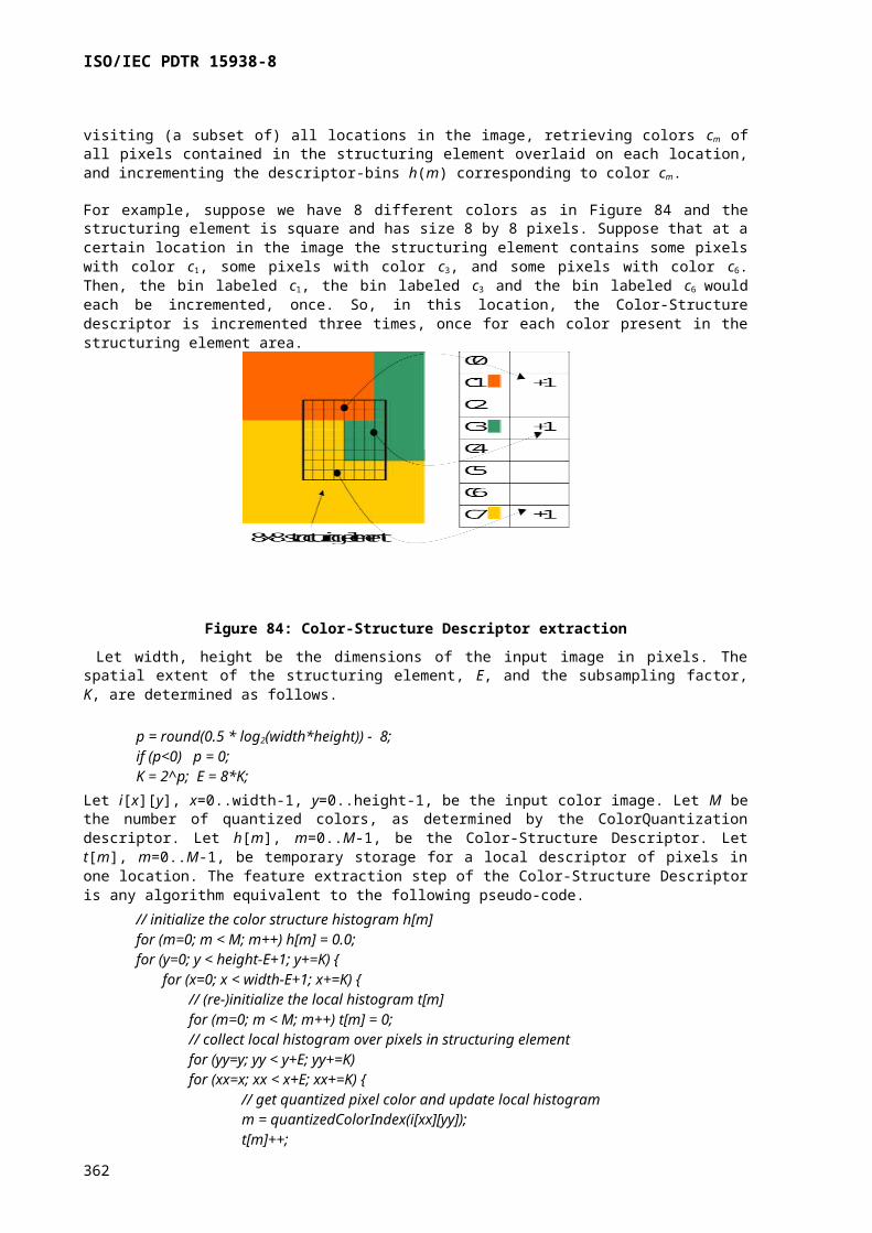
Figure 125: Correlation imagesIf the maximum value of the face correlation for a candidate face image is above a certain threshold the candidate face image is confirmed as a true face image.
5.7.1.1.1.4.3 Elimination of false positives
Once a candidate face image has been confirmed as a true face using the face correlation, two test are performed to eliminate regions which have been falsely confirmed as faces. The first of these tests determines if the spatial distribution of horizontal and vertical valleys and ridges match the distribution for a face. To perform this test the four valley and ridge images are divided up into 36 regions as shown in Figure 126. The pixel values of these 36 regions are then summed to give 36 partial sums xi
(i = 0, …,36). A linear combination of these partial sums is then calculated and compared against a threshold. If the linear combination is below the threshold the face candidate is rejected.1 2 3
4 5 6
7 8 9
10 11 12
13 14 15
16 17 18
19 20 21
22 23 24
25 26 27
28 29 30
31 32 33
34 35 36
TVH TRH TVV TRV
Figure 126: Sub-regions for spatial distribution calculationThe second test for false positives uses the chrominance information in the image and can only be carried out on colour images. For each candidate face region, the average U and V values are calculated and given by Uave and Vave . The angle which these two average chrominance values represent in the UV plane is then calculated using the equation
.
If this angle is less than 1050 or greater than 1640 then the face candidate is rejected.
5.7.1.2 Similarity matching
The similarity of face images is defined as the weighted distance between normalized projections:
The suggested weights are as follows:
365

Annex A Patent Statements
MPEG-7
Patent Statements
Sys DDL Visual Audio MDS Ref. Sof.
Canon X
CIE X X X X X X
Denso X X
ETRI X X X X X X
Expway X X X X X X
FhG X
Fraunhofer X
Geocast X X X X X
HHI X X
Hitachi X X X X X X
Hyundai X X X
IBM X X X X X X
JVC X X X X X X
KDDI X X X X
LG Electronics X X X X X X
Matsushita X X X X X X
Mitsubishi Electric X X X X X X
NEC
NHK X X X X X X
Philips X X X X X X
Ricoh X X X X X X
Samsung X X X X X X
366

Sharp X X X X X
Siemens X X X X X X
Sony X X X X X X
Toshiba X X X X X X
Vivcom X X
367

Bibliography
ISO 8601, Data elements and interchange formats – Information interchange – Representation of dates and times.
ISO 639, Code for the representation of names of languages.
ISO 3166-1, Codes for the representation of names of countries and their subdivisions – Part 1: Country codes.
ISO 3166-2, Codes for the representation of names of countries and their subdivisions – Part 2: Country subdivision code.
ISO 4217, Codes for the representation of currencies and funds.
ISO/IEC 11172 Information technology – Coding of moving pictures and associated audio for digital storage media at up to about 1,5 Mbit/s.
ISO/IEC 13818, Information technology – Generic coding of moving pictures and associated audio information.
ISO/IEC 14496, Information technology – Coding of audio-visual objects.
ISO/IEC 15938-1, Information technology – Multimedia Content Description Interface: Systems.
ISO/IEC 15938-2, Information technology – Multimedia Content Description Interface: Description Definition Langauge.
ISO/IEC 15938-3, Information technology – Multimedia Content Description Interface: Visual.
ISO/IEC 15938-4, Information technology – Multimedia Content Description Interface: Audio.
ISO/IEC 15938-6, Information technology – Multimedia Content Description Interface: Reference Software.
XML, Extensible Markup Language, W3C Recommendation, World Wide Web Consortium (W3C).
XML Schema, XML Schema, W3C Recommendation, World Wide Web Consortium (W3C).
xPath, XML Path Language, W3C Recommendation, World Wide Web Consortium (W3C).
RFC 2396, Uniform Resource Identifiers (URI): Generic Syntax, The Internet Engineering Task Force (IETF).
RFC 2045, Multipurpose Internet Mail Extensions (MIME) Part One: Format of Internet Message Bodies, The Internet Engineering Task Force (IETF).
RFC 2046, Multipurpose Internet Mail Extensions (MIME) Part Two: Media Types, The Internet Engineering Task Force (IETF).
RFC 2048, Multipurpose Internet Mail Extensions (MIME) Part Four: Registration Procedures, The Internet Engineering Task Force (IETF).
RFC 2045-CHARSETS, Registered Character set codes of RFC2045, The Internet Engineering Task Force (IETF).
RFC 2046-MIMETYPES, Registered Mimetypes of RFC2046, The Internet Engineering Task Force (IETF).
368

Special issue on Object Based Video Coding and Description, IEEE Transactions on Circuits and Systems for Video Technology, 9(8), December 1999.
L. Agnihotri and N. Dimitrova, "Text Detection for Video Analysis", Workshop on Content Based Image and Video Libraries, held in conjunction with CVPR, Colorado, pp. 109-113, 1999.
Y. Abdeljaoued , T. Ebrahimi, C. Christopoulos, I. Mas Ivars, "A new algorithm for shot boundary detection", Proceedings European Signal Processing Conference (EUSIPCO 2000), Special session on Multimedia Indexing, Browsing and Retrieval, 5-8 September 2000, Tampere, Finland.
M. Bierling, "Displacement Estimation by Hierarchical Block Matching", SPIE Vol 1001, Visual Communication & Image Processing, 1988.
A. D. Bimbo, E. Vicario and D. Zingoni, "Symbolic description and visual querying of image sequences using spatio-temporal logic", IEEE Transactions on Knowledge and Data Engineering, Vol 7, No. 4, August, 1995.
N. Björk and Christopoulos C., "Transcoder Architectures for video coding", Proceedings of IEEE International Conference on Acoustic Speech and Signal Processing (ICASSP 98), Seattle, Washington, Vol. 5, pp. 2813-2816, May 12-15, 1998.
S.-K. Chang, Q. Y. Shi, and C. Y. Yan, "Iconic indexing by 2-D strings", IEEE Trans. Pattern Analysis Machine Intell., 9(3):413-428, May 1987.
N. Damera-Venkata, etal, "Image quality assessment based on a degradation model," IEEE Trans. Image Processing, vol. 9, no. 4, pp. 636-650, 2000.
G. Freytag, “Technique of the Drama”, 2ed, ed. Translated by Elias J. MacEwan, Chicago: Scott, Foresman, 1898
V.N. Gudivada and V.V. Raghavan, "Design and Evaluation of ALgorithms for Image Retrieval by Spatial Similarity", ACM Transaction on Information Systems, Vol.13,No,2,April 1995, pp.115-144.
A. Hanjalic, H.J. Zhang, an integrated scheme for automated video abstraction based on unsupervised cluster-validity analysis, IEEE Transactions on Circuits and Systems for Video Technology 9(8): 1280-1289, December 1999.
M. Kass, A. Witkin and D. Terzopoulos, "Snakes: Active contour models", International Journal of Computer Vision, pp 321-331, 1988.
M. Kim, J.G. Choi, D. Kim, H. Lee, M.H. Lee, C. Ahn, Y.S. Ho, A VOP Generation tool: automatic segmentation of moving objects in image sequences based on spatio-temporal information, IEEE Transactions on Circuits and Systems for Video Technology 9(8): 1216-1226, December 1999.
P. Kuhn: "Algorithms, Complexity Analysis and VLSI-Architectures for MPEG-4 Motion Estimation", Kluwer Academic Publishers, 1999, ISBN 792385160.
P. Kuhn: "Camera Motion Estimation using feature points in MPEG compressed domain", IEEE International Conference on Image Processing (ICIP), September 10-13, 2000, Vancouver, Canada
S. Herrmann, H. Mooshofer, HY. Dietrich, W. Stechele, A video segmentation algorithm for hierarchical object representation and its implementation, IEEE Transactions on Circuits and Systems for Video Technology 9(8): 1204-1215, December 1999.
Jain AK, Dubes RC. Algorithms for clustering data. Prentice Hall, Englewood Cliffs, NJ, 1988.
B. Laurel, “Computers as Theatre”, Addison-Wesley, 1993
369

T. Meier, K. N. Ngan, Video segmentation for content based coding, IEEE Transactions on Circuits and Systems for Video Technology 9(8): 1190-1203, December 1999.
J. Meng, Y. Juan and S.-F. Chang, Scene Change Detection in a MPEG Compressed Video Sequence, Proceedings, IS&T/SPIE's Symposium on Electronic Imaging: Science & Techno logy (EI'95) – Digital Video Compression: Algorithms and Technologies, San Jose, February 1995.
A. Perkis, Y. Abdeljaoued , C. Christopoulos, T. Ebrahimi, J. Chicharo, "Universal Multimedia Access from Wired and Wireless Systems", submitted to Circuits, Systems and Signal Processing, Special Issue on Multimedia Communication Services, 2000.
P. Salembier and F. Marqués, Region-based representation of image and video: Segmentation tools for multimedia services, IEEE Transactions on Circuits and Systems for Video Technology 9(8): 1147-1169, December 1999.
J-C. Shim, C. Dorai, and R. Bolle, "Automatic Text Extraction from Video for Content-Based Annotation and Retrieval," in Proc. of the Int. Conference on Pattern Recognition, pp. 618-620, August 1998.
J.-C. Shim and C. Dorai, "A Fast and Generalized Region Labeling Algorithm," in Proc. of the Int. Conference on Image Processing, October 1999.
H. Wallin , C. Christopoulos, A. Smolic, Y. Abdeljaoued, T. Ebrahimi, "Robust mosaic construction algorithm", ISO/IEC JTC1/SC29/WG11 MPEG00/M5698, Noordwijkerhout, The Netherlands, March 2000.
World Wide Web Consortium (W3C), "Synchronized Multimedia", http://www.w3.org/AudioVideo/
D. Zhong and S.-F. Chang, "AMOS: An Active System For MPEG-4 Video Object Segmentation", 1998 International Conference on Image Processing, October 4-7, 1998, Chicago, Illinois, USA
D. Zhong and S.-F.Chang, "Video Object Model and Segmentation for Content-Based Video Indexing", ISCAS’97, HongKong, June 9-12, 1997
D. Zhong and S.-F.Chang, "Spatio-Temporal Video Search Using the Object Based Video Representation", ICIP'97, October 26-29, 1997 Santa Barbara, CA
D. Zhong and S.-F. Chang, "Region Feature Based Similarity Searching of Semantic Video Objects", ICIP'99, Oct 24-28 1999, Kobe, Japan.
J. F. Allen. Maintaining knowledge about temporal intervals. Communication of ACM, 26(11):832-843, 1983.
S.-K. Chang, Q. Y. Shi, and C. Y. Yan, "Iconic indexing by 2-D strings", IEEE Trans. Pattern Analysis Machine Intell., 9(3):413-428, May 1987.
Dewey Decimal system, http://www.oclc.org/dewey/
S.C. Shapiro, "Encyclopedia of Artificial Intelligence Second Edition", Vol.2, pp.1495, Wiley-Interscience, 1992
Yeun-Bae Kim, Masahiro Shibata, "A Video Indexing Method using Natural Language Memo for TV Program Production", pp.266-270, Proceedings of ECAI96, 12th European Conference on Artificial Intelligence, August 1996.
Y. Takahashi, K. Hasegawa, K. Sugiyama, M. Watanabe, "Describing Story Structure of Movies with Semantic Score Method - Toward Human Content Interface Design (3) -", Bulletin of Japanese Society for Science of Design, Vol.46, No.6, pp57-66 (2000) (in Japanese)
Gustav Freytag, “Technique of the Drama”, 2ed, ed. Translated by Elias J. MacEwan, Chicago: Scott, Foresman, 1898.
370

Brenda Laurel, “Computers as Theatre”, Addison-Wesley, 1993.
Yasushi Takahashi, Yoshiaki Shibata, Mikio Kamada and Hitoshi Kimura, “The Semantic Score Method: A standard tool for quantitative content evaluation by multiple viewers”, submitted to International Conference on Media Futures (2001).
Y. Takahashi, "Semantic Score Method: A Standardized Tool for Quantitative Movie Interpretation - Toward Human Content Interface Design(5) -", Bulletin of JSSD,Vol.47, No.4, (2000) (in Japanese)
Y. Takahashi, K. Hasegawa, K. Sugiyama, M. Watanabe, "A New Movie Summarization Algorithm for Effective Movie Selection - Toward Human Content Interface Design(4) -", Bulletin of JSSD,Vol.47, No.4, (2000) (in Japanese)
M. Lounsberry, T. DeRose, J. Warren, “Multiresolution analysis for surfaces of arbitrary topological type”, TR 93-10-05b, Dept. of CS & Eng., univ of Washington, January 94.
371


![TUTORIAL SU MPEG-7 [ISO/IEC 15938] - LIM | … VERCELLESI (giancarlo.vercellesi@dico.unimi.it) TUTORIAL SU MPEG-7 [ISO/IEC 15938] L.I.M. - Laboratorio di Informatica Musicale DICo](https://static.fdocuments.net/doc/165x107/5c68c98509d3f290788c0f1b/tutorial-su-mpeg-7-isoiec-15938-lim-vercellesi-dicounimiit-tutorial.jpg)


![TUTORIAL SU MPEG-7 [ISO/IEC 15938] - unimi.it](https://static.fdocuments.net/doc/165x107/61facaa8c999102dc55e3689/tutorial-su-mpeg-7-isoiec-15938-unimiit.jpg)

![ISO/IEC JTC 1/SC 29 N - Moving Picture Experts Group · Web view[1]ISO/IEC 15938-9:2005/Amd 1:2012, “Extensions to profiles and levels”, 2012. [2]ISO/IEC TR 15938-11:2005/Amd](https://static.fdocuments.net/doc/165x107/613691450ad5d20676481c31/isoiec-jtc-1sc-29-n-moving-picture-experts-group-web-view-1isoiec-15938-92005amd.jpg)


