Basic Sampling Methods - University at Buffalosrihari/CSE574/Chap11/Ch11.2...Basic Sampling Methods...

Machine Learning Srihari

1

Basic Sampling Methods

Sargur [email protected]


2

Topics1. Motivation2. Sampling from PGMs3. Transforming a Uniform Distribution4. Rejection Sampling5. Importance Sampling6. Sampling-Importance-Resampling


3

1. Motivation• Inference is the task of determining a response to a

query from a given model• When exact inference is intractable, we need some

form of approximation• Inference methods based on numerical sampling are

known as Monte Carlo techniques• Most situations will require evaluating expectations of

unobserved variables, e.g., to make predictions


4

Using samples for inference• Obtain set of samples z(l) where i =1,.., L• Drawn independently from distribution p(z)• Allows expectation to be approximated by

– Then , i.e., estimator has the correct mean – And which is the variance of the estimator

• Accuracy independent of dimensionality of z– High accuracy can be achieved with few (10 or 20 samples)

• However samples may not be independent– Effective sample size may be smaller than apparent sample size– In example f(z) is small when p(z) is high and vice versa

• Expectation may be dominated by regions of small probability thereby requiring large sample sizes

f = 1

Lf (z (l ))

i=1

L

∑ Called an estimator

E[ f ] = E[f ]

var[ f ]= 1LE f −E( f )( )2"#

$%

E[f ] = f (z)p(z)dz∫


5

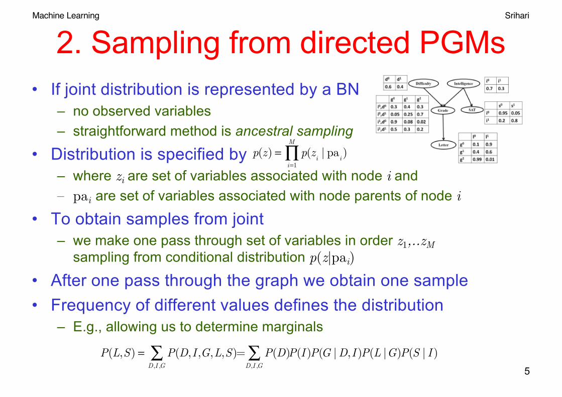
2. Sampling from directed PGMs• If joint distribution is represented by a BN

– no observed variables– straightforward method is ancestral sampling

• Distribution is specified by– where zi are set of variables associated with node i and – pai are set of variables associated with node parents of node i

• To obtain samples from joint – we make one pass through set of variables in order z1,..zM

sampling from conditional distribution p(z|pai)

• After one pass through the graph we obtain one sample• Frequency of different values defines the distribution

– E.g., allowing us to determine marginals

p(z) = p(z

i| pa

i)

i=1

M

∏

P(L,S) = P(D,I ,G,L,S)

D,I ,G∑ = P(D)

D,I ,G∑ P(I )P(G |D,I )P(L |G)P(S | I )


6

Ancestral sampling with some nodes instantiated

• Directed graph where some nodes instantiated with observed values

• Called Logic sampling• Use ancestral sampling, except

– When sample is obtained for an observed value:• if they agree then sample value is retained and proceed

to next variable• If they don’t agree, whole sample is discarded

P(L= l0 ,s = s1)=P(D)P(I)P(G |D,I)

D ,I ,G∑ ×

P(L= l0 |G)P(S = s1 |I)


7

Properties of Logic Sampling

• Samples correctly from posterior distribution– Corresponds to sampling from joint distribution of

hidden and data variables• But prob. of accepting sample decreases as

– no of variables increase and – number of states that variables can take increases

• A special case of Importance Sampling– Rarely used in practice

P(L = l0, s = s1) =

P(D)P(I )P(G |D, I )D,I ,G∑ ×

P(L = l0 |G)P(S = s1 | I )


8

Undirected Graphs

• No one-pass sampling strategy even from prior distribution with no observed variables

• Computationally expensive methods such as Gibbs sampling must be used– Start with a sample– Replace first variable conditioned on rest of values,

then next variable, etc


9

3. Basic Sampling Algorithms• Simple strategies for generating random samples from

a given distribution• Assume that algorithm is provided with a pseudo-

random generator for uniform distribution over (0,1)• For standard distributions we can use transformation

method of generating non-uniformly distributed random numbers


Transformation Method• Goal: generate random numbers from a simple

non-uniform distribution• Assume we have a source of uniformly

distributed random numbers• z is uniformly distributed over (0,1), i.e., p(z) =1

in the interval

10

0 1

p(z)z


Inverse Probability Transform• Let F(x) be a cumulative distribution function of

some distribution we want to sample from• Let F-1(u) be its inverse then we have

• Theorem:– If u~U(0,1) is a uniform random variable then F-1(u)~F

– Proof:• P(F-1(u)≤ x)=P(u ≤ F(x)) applying F to both sides of lhs

=F(x) because P(u≤y)=y and since u is uniform on unit interval

11

0 x0

u

1 F

F -1


Transformation for Standard Distributions

(1) )()(dydzzpyp =

z = h(y) ≡ p(y)−∞

y

∫ dy

0 1z y = f(z)

f(z)

p(z) p(y)


13

Geometry of Transformation• We are interested in generating r.v. s from p(y)

– non-uniform random variables

• h(y) is indefinite integral of desired p(y)• z ~ U(0,1) is transformed using y = h-1(z)• Results in y being distributed as p(y)


14

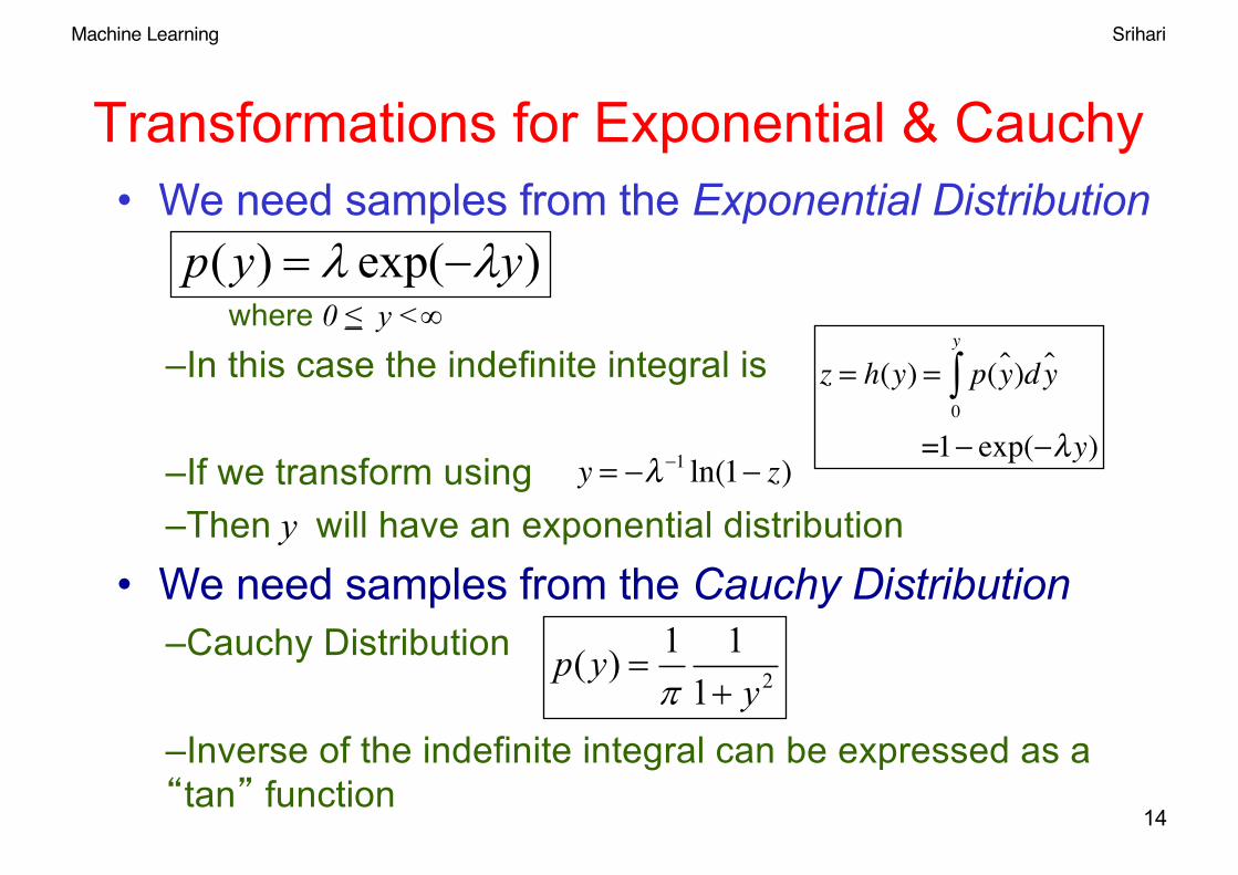
Transformations for Exponential & Cauchy • We need samples from the Exponential Distribution

where 0 ≤ y <∞

–In this case the indefinite integral is

–If we transform using –Then y will have an exponential distribution

• We need samples from the Cauchy Distribution–Cauchy Distribution

–Inverse of the indefinite integral can be expressed as a �tan� function

)exp()( yyp ll -=

z = h(y) = p(y )dy0

y

∫ =1− exp(−λy)

y = −λ−1 ln(1− z)

2111)(y

yp+

=p


Generalization of Transformation Method

• Single variable transformation

– Where z is uniformly distributed over (0,1)• Multiple variable transformation

15

p(y) = p(z) dzdy

p(y1,...., yM ) = p(z1,..., zM ) d(z1,..., zM )d(y1,..., yM )


16

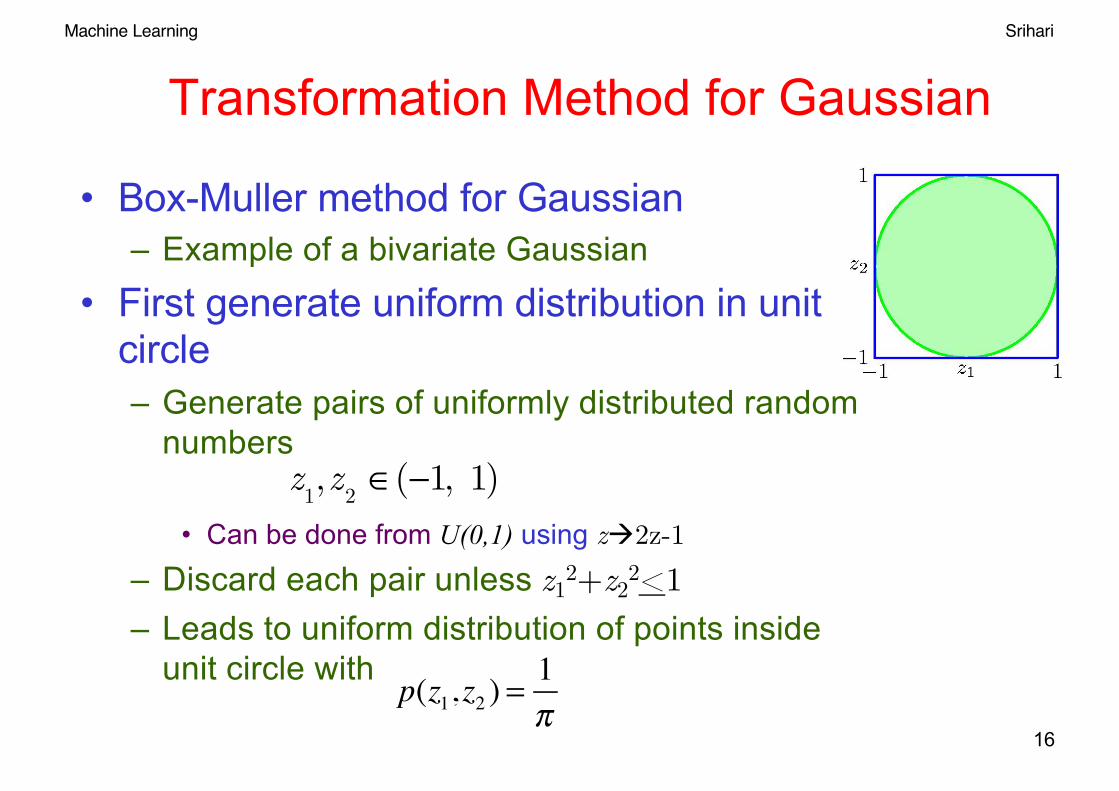
Transformation Method for Gaussian

• Box-Muller method for Gaussian– Example of a bivariate Gaussian

• First generate uniform distribution in unit circle– Generate pairs of uniformly distributed random

numbers

• Can be done from U(0,1) using zà2z-1– Discard each pair unless z12+z22<1– Leads to uniform distribution of points inside

unit circle with

z1,z

2∈(−1, 1)

p(z1, z2 ) =1π


17

Generating a Gaussian• For each pair z1,z2 evaluate the quantities

– Then y1 and y2 are independent Gaussians with zero mean and variance

• For arbitrary mean and covariance matrix

• In multivariate case

22

21

2

2/1

22

22

2/1

21

11

zzr

ln2 ln2

+=

÷øö

çèæ -=÷

øö

çèæ -=

whererzzy

rzzy

If y N(0,1) then σ y + µ has N(µ,σ 2 )

If components are independent and N 0,1( )then y = µ + Lzwill have N(µ,Σ) where Σ = LLT , is called the Cholesky decomposition


Limitation of Transformation Method

• Need to first calculate and then invert indefinite integral of the desired distribution

• Feasible only for a small number of distributions

• Need alternate approaches• Rejection sampling and Importance sampling

applicable to univariate distributions only– But useful as components in more general

strategies18


19

4. Rejection Sampling• Allows sampling from a relatively complex distribution• Consider univariate, then extend to several variables• Wish to sample from distribution p(z)

– Not a simple standard distribution– Sampling from p(z) is difficult

• Suppose we are able to easily evaluate p(z) for any given value of z, upto a normalizing constant Zp

– where can readily be evaluated but Zp is unknown– e.g., is a mixture of Gaussians

– Note that we may know the mixture distribution but we need samples to generate expectations

p(z) = 1Zp

p(z)

p(z)

Unnormalized

p(z)


Rejection sampling: Proposal distribution

• Samples are drawn from simple distribution, called proposal distribution q(z)

• Introduce constant k whose value is such that for all z

– Called comparison function

20

kq(z) ≥ p(z)


21

Rejection Sampling Intuition• Samples are drawn from

simple distribution q(z)• Rejected if they fall in grey

area– Between un-normalized

distribution p~(z) and scaled distribution kq(z)

• Resulting samples are distributed according to p(z)which is the normalized version of p~(z)


22

Determining if sample is shaded area• Generate two random numbers

– z0 from q(z) – u0 from uniform distribution [0,kq(z0)]

• This pair has uniform distribution under the curve of function kq(z)

• If the pair is rejected otherwise it is retained

• Remaining pairs have a uniform distribution under the curve of p(z) and hence the corresponding z values are distributed according to p(z) as desired

u0 > p(z0 )


23

Example of Rejection Sampling• Task of sampling from

Gamma

• Since Gamma is roughly bell-shaped, proposal distribution is is Cauchy

• Cauchy has to be slightly generalized – To ensure it is nowhere

smaller than Gamma

)()exp(

),|(1

abzzbbazGam

aa

G-

=-

Gamma

ScaledCauchy


24

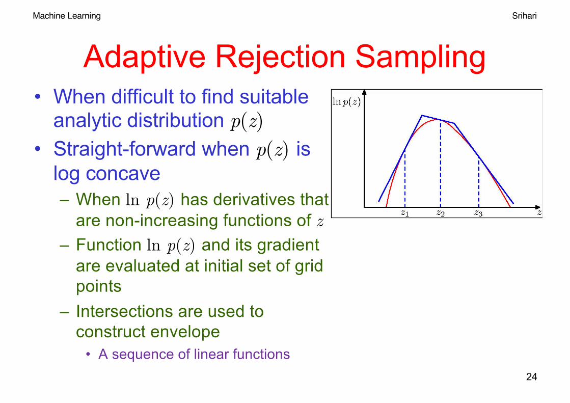
Adaptive Rejection Sampling• When difficult to find suitable

analytic distribution p(z)• Straight-forward when p(z) is

log concave– When ln p(z) has derivatives that

are non-increasing functions of z– Function ln p(z) and its gradient

are evaluated at initial set of grid points

– Intersections are used to construct envelope

• A sequence of linear functions


25

Dimensionality and Rejection Sampling

• Gaussian example• Acceptance rate is

ratio of volumes under p(z) and kq(z)– diminishes

exponentially with dimensionality

Proposal distribution q(z) is GaussianScaled version is kq(z)

True distribution p(z)


26

5. Importance Sampling• Principal reason for sampling p(z) is evaluating

expectation of some f(z)

• Given samples z(l), l=1,..,L, from p(z), the finite sum approximation is

• But drawing samples p(z) may be impractical• Importance sampling uses:

– a proposal distribution– like rejection sampling • But all samples are retained

– Assumes that for any z, p(z) can be evaluated

E[f ] = f (z)p(z)dz∫

f = 1

Lf (z (l ))

i=1

L

∑

p(t | x)= p(t|x,w)p(w)dw∫

In Bayesian regression,

wherep(t |x,w)~N(y(x,w),β-1)


Determining Importance weights

• Sample {z(l)} from a simpler distribution q(z)

• Samples are weighted by ratios rl= p(z(l)) / q(z(l))

– Known as importance weights• Which corrects the bias introduced by wrong distribution

27

Proposal distribution

E[f ] = f (z)p(z)dz∫ = f (z)

p(z)q(z)

q(z)dz∫

=1L

p(z (l ))q(z (l ))l=1

L

∑ f (z (l )) Unlike rejection samplingall of the samples are retained


Likelihood-weighted Sampling

• Importance sampling of graphical model using ancestral sampling

• Weight of sample z given evidence variables E

28

r(z) = p(zi | pai )zi∈E∏


29

6. Sampling-Importance Re-sampling (SIR)

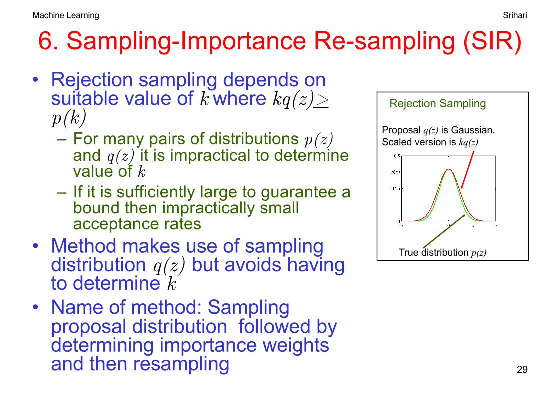
• Rejection sampling depends on suitable value of k where kq(z)> p(k)– For many pairs of distributions p(z)

and q(z) it is impractical to determine value of k

– If it is sufficiently large to guarantee a bound then impractically small acceptance rates

• Method makes use of sampling distribution q(z) but avoids having to determine k

• Name of method: Sampling proposal distribution followed by determining importance weights and then resampling

Proposal q(z) is Gaussian. Scaled version is kq(z)

True distribution p(z)

Rejection Sampling


30

SIR Method• Two stages• Stage 1: L samples z(1),..,z(L) are drawn from

q(z)• Stage 2: Weights w1,..,wL are constructed

– As in importance sampling wl= p(z(l)) / q(z(l))• Finally a second set of L samples are drawn

from the discrete distribution {z(1),..,z(L) } with probabilities given by {w1,..,wL}

• If moments wrt distribution p(z) are needed, use: E[ f ]= f (z)p(z)dz∫

= wll=1

L

∑ f (z(l ) )

Basic Sampling Methods - University at Buffalosrihari/CSE574/Chap11/Ch11.2...Basic Sampling Methods...

Documents

Transcript of Basic Sampling Methods - University at Buffalosrihari/CSE574/Chap11/Ch11.2...Basic Sampling Methods...