CS 450 : Operating Systems Michael Saelee <lee@iit.edu>

Basic Queueing Theory

- Queueing theory? Huh?

- Probability refresher / Crash course

- Queueing theory & Kendall’s notation

- Mean value analysis of basic queues

Agenda

§ Queueing Theory? Huh?

Remember, we started our discussion of scheduling at a high level — “policy”

- mostly described heuristics-based (i.e., hand-wavy) approaches

to obtain empirical data, we can examine a “live” operating system’s scheduler

to exercise rigor, should leverage some branch of mathematics well-suited to analyzing scheduling systems … queueing theory!

queueing theory models wait queues using probability theory - e.g., arrival/service rate distributions - supports mathematical analysis & rigor

wide application: - checkout lines

- telecom switch

- traffic light system

- network quality of service

we’ll barely scratch the surface — queueing theory is an area ripe for research — but you’ll see some basic applications

- will also help explain underpinnings of simulators used for scheduling!

§ Probability refresher / Crash course

Probability theory = quantitative analysis of random phenomena - assign a weighted probability to every event in a sample space (Ω) - use these probability distributions to better understand the behavior of the phenomena

Core abstraction: random variable - a R.V. is a function that maps the sample space onto numeric

values (e.g., X:Ω→ℝ)

- discrete R.V.s map to a countable set

- continuous R.V.s map events onto an uncountable set (e.g., real-valued)

⌦ = {TT, TH,HT,HH}

X(!) =

8>><

>>:

0, if ! = TT

1, if ! = TH

2, if ! = HT

3, if ! = HH

E.g., double coin toss (discrete event space)

Typically interested in a variety of statistics of random variables (and corresponding events):

- probability of event n: P(X=n) (or p(n))

- expected value (mean): E(X)

- variance: σ2(X); standard deviation: σ(X)

- coefficient of variance: CX=σ(X)/E(X)(unitless measure)

e.g., 6-sided dice roll

— probability mass function

Note:X

n

P (X = n) = 1

E(X) =X

n

n · p(n) = 3.5

P (X = n) = p(n) =1

6, n = 1, 2, 3, 4, 5, 6

<latexit sha1_base64="33hdbwTSVxBON+FiA5gMGQhY0lE=">AAACD3icbZDLSgMxFIYz9VbrbdSlm2BRKgxlptbqplB047KCvUA7lEyaaUMzmSHJCGXoG7jxVdy4UMStW3e+jWk7C209kPDx/+eQnN+LGJXKtr+NzMrq2vpGdjO3tb2zu2fuHzRlGAtMGjhkoWh7SBJGOWkoqhhpR4KgwGOk5Y1upn7rgQhJQ36vxhFxAzTg1KcYKS31zNN6oV3lZ9WooK+uLxBOnElSmViQVx2rZJ1bZevCqvTMvF20ZwWXwUkhD9Kq98yvbj/EcUC4wgxJ2XHsSLkJEopiRia5bixJhPAIDUhHI0cBkW4y22cCT7TSh34o9OEKztTfEwkKpBwHnu4MkBrKRW8q/ud1YuVfuQnlUawIx/OH/JhBFcJpOLBPBcGKjTUgLKj+K8RDpENROsKcDsFZXHkZmqWio/munK9dp3FkwRE4BgXggEtQA7egDhoAg0fwDF7Bm/FkvBjvxse8NWOkM4fgTxmfP/s6mMs=</latexit><latexit sha1_base64="33hdbwTSVxBON+FiA5gMGQhY0lE=">AAACD3icbZDLSgMxFIYz9VbrbdSlm2BRKgxlptbqplB047KCvUA7lEyaaUMzmSHJCGXoG7jxVdy4UMStW3e+jWk7C209kPDx/+eQnN+LGJXKtr+NzMrq2vpGdjO3tb2zu2fuHzRlGAtMGjhkoWh7SBJGOWkoqhhpR4KgwGOk5Y1upn7rgQhJQ36vxhFxAzTg1KcYKS31zNN6oV3lZ9WooK+uLxBOnElSmViQVx2rZJ1bZevCqvTMvF20ZwWXwUkhD9Kq98yvbj/EcUC4wgxJ2XHsSLkJEopiRia5bixJhPAIDUhHI0cBkW4y22cCT7TSh34o9OEKztTfEwkKpBwHnu4MkBrKRW8q/ud1YuVfuQnlUawIx/OH/JhBFcJpOLBPBcGKjTUgLKj+K8RDpENROsKcDsFZXHkZmqWio/munK9dp3FkwRE4BgXggEtQA7egDhoAg0fwDF7Bm/FkvBjvxse8NWOkM4fgTxmfP/s6mMs=</latexit><latexit sha1_base64="33hdbwTSVxBON+FiA5gMGQhY0lE=">AAACD3icbZDLSgMxFIYz9VbrbdSlm2BRKgxlptbqplB047KCvUA7lEyaaUMzmSHJCGXoG7jxVdy4UMStW3e+jWk7C209kPDx/+eQnN+LGJXKtr+NzMrq2vpGdjO3tb2zu2fuHzRlGAtMGjhkoWh7SBJGOWkoqhhpR4KgwGOk5Y1upn7rgQhJQ36vxhFxAzTg1KcYKS31zNN6oV3lZ9WooK+uLxBOnElSmViQVx2rZJ1bZevCqvTMvF20ZwWXwUkhD9Kq98yvbj/EcUC4wgxJ2XHsSLkJEopiRia5bixJhPAIDUhHI0cBkW4y22cCT7TSh34o9OEKztTfEwkKpBwHnu4MkBrKRW8q/ud1YuVfuQnlUawIx/OH/JhBFcJpOLBPBcGKjTUgLKj+K8RDpENROsKcDsFZXHkZmqWio/munK9dp3FkwRE4BgXggEtQA7egDhoAg0fwDF7Bm/FkvBjvxse8NWOkM4fgTxmfP/s6mMs=</latexit><latexit sha1_base64="ck8pdC+ekZH4nUmSP+ZG7r8lEyk=">AAAB2XicbZDNSgMxFIXv1L86Vq1rN8EiuCozbnQpuHFZwbZCO5RM5k4bmskMyR2hDH0BF25EfC93vo3pz0JbDwQ+zknIvSculLQUBN9ebWd3b/+gfugfNfzjk9Nmo2fz0gjsilzl5jnmFpXU2CVJCp8LgzyLFfbj6f0i77+gsTLXTzQrMMr4WMtUCk7O6oyaraAdLMW2IVxDC9YaNb+GSS7KDDUJxa0dhEFBUcUNSaFw7g9LiwUXUz7GgUPNM7RRtRxzzi6dk7A0N+5oYkv394uKZ9bOstjdzDhN7Ga2MP/LBiWlt1EldVESarH6KC0Vo5wtdmaJNChIzRxwYaSblYkJN1yQa8Z3HYSbG29D77odOn4MoA7ncAFXEMIN3MEDdKALAhJ4hXdv4r15H6uuat66tDP4I+/zBzjGijg=</latexit><latexit sha1_base64="17UuOYqWZInhVmp/m7fMJfwWJtk=">AAACBHicbZDLSgMxGIX/qbdaq45u3QSLUmEoM1Wrm4LgxmUFe4G2lEyaaUMzmSHJCGXoG7jxVdy4UMRncOfbmF4W2nog4eOchOQ/fsyZ0q77bWXW1jc2t7LbuZ387t6+fZBvqCiRhNZJxCPZ8rGinAla10xz2oolxaHPadMf3U7z5iOVikXiQY9j2g3xQLCAEayN1bNPa8VWVZxV46LZOoHEJPUmaWXiIFH1nLJz7lw4l06lZxfckjsTWgVvAQVYqNazvzr9iCQhFZpwrFTbc2PdTbHUjHA6yXUSRWNMRnhA2wYFDqnqprN5JujEOH0URNIsodHM/X0jxaFS49A3J0Osh2o5m5r/Ze1EB9fdlIk40VSQ+UNBwpGO0LQc1GeSEs3HBjCRzPwVkSE2pWhTYc6U4C2PvAqNcskzfO9CFo7gGIrgwRXcwB3UoA4EnuAF3uDderZerY95XRlr0dsh/JH1+QNrsZdR</latexit><latexit sha1_base64="17UuOYqWZInhVmp/m7fMJfwWJtk=">AAACBHicbZDLSgMxGIX/qbdaq45u3QSLUmEoM1Wrm4LgxmUFe4G2lEyaaUMzmSHJCGXoG7jxVdy4UMRncOfbmF4W2nog4eOchOQ/fsyZ0q77bWXW1jc2t7LbuZ387t6+fZBvqCiRhNZJxCPZ8rGinAla10xz2oolxaHPadMf3U7z5iOVikXiQY9j2g3xQLCAEayN1bNPa8VWVZxV46LZOoHEJPUmaWXiIFH1nLJz7lw4l06lZxfckjsTWgVvAQVYqNazvzr9iCQhFZpwrFTbc2PdTbHUjHA6yXUSRWNMRnhA2wYFDqnqprN5JujEOH0URNIsodHM/X0jxaFS49A3J0Osh2o5m5r/Ze1EB9fdlIk40VSQ+UNBwpGO0LQc1GeSEs3HBjCRzPwVkSE2pWhTYc6U4C2PvAqNcskzfO9CFo7gGIrgwRXcwB3UoA4EnuAF3uDderZerY95XRlr0dsh/JH1+QNrsZdR</latexit><latexit sha1_base64="ZzSe56npIEy+O0YUG4qA/G13BGU=">AAACD3icbZBNS8MwGMdTX+d8q3r0EhzKhDLaqdPLYOjF4wT3AlsZaZZuYWlaklQYpd/Ai1/FiwdFvHr15rcx23rQzQcSfvz/z0Py/L2IUals+9tYWl5ZXVvPbeQ3t7Z3ds29/aYMY4FJA4csFG0PScIoJw1FFSPtSBAUeIy0vNHNxG89ECFpyO/VOCJugAac+hQjpaWeeVIvtqv8tBoV9dX1BcKJkyaV1IK86lhl68w6ty6sSs8s2CV7WnARnAwKIKt6z/zq9kMcB4QrzJCUHceOlJsgoShmJM13Y0kihEdoQDoaOQqIdJPpPik81kof+qHQhys4VX9PJCiQchx4ujNAaijnvYn4n9eJlX/lJpRHsSIczx7yYwZVCCfhwD4VBCs21oCwoPqvEA+RDkXpCPM6BGd+5UVolkuO5ju7ULvO4siBQ3AEisABl6AGbkEdNAAGj+AZvII348l4Md6Nj1nrkpHNHIA/ZXz+APn6mMc=</latexit><latexit sha1_base64="33hdbwTSVxBON+FiA5gMGQhY0lE=">AAACD3icbZDLSgMxFIYz9VbrbdSlm2BRKgxlptbqplB047KCvUA7lEyaaUMzmSHJCGXoG7jxVdy4UMStW3e+jWk7C209kPDx/+eQnN+LGJXKtr+NzMrq2vpGdjO3tb2zu2fuHzRlGAtMGjhkoWh7SBJGOWkoqhhpR4KgwGOk5Y1upn7rgQhJQ36vxhFxAzTg1KcYKS31zNN6oV3lZ9WooK+uLxBOnElSmViQVx2rZJ1bZevCqvTMvF20ZwWXwUkhD9Kq98yvbj/EcUC4wgxJ2XHsSLkJEopiRia5bixJhPAIDUhHI0cBkW4y22cCT7TSh34o9OEKztTfEwkKpBwHnu4MkBrKRW8q/ud1YuVfuQnlUawIx/OH/JhBFcJpOLBPBcGKjTUgLKj+K8RDpENROsKcDsFZXHkZmqWio/munK9dp3FkwRE4BgXggEtQA7egDhoAg0fwDF7Bm/FkvBjvxse8NWOkM4fgTxmfP/s6mMs=</latexit><latexit sha1_base64="33hdbwTSVxBON+FiA5gMGQhY0lE=">AAACD3icbZDLSgMxFIYz9VbrbdSlm2BRKgxlptbqplB047KCvUA7lEyaaUMzmSHJCGXoG7jxVdy4UMStW3e+jWk7C209kPDx/+eQnN+LGJXKtr+NzMrq2vpGdjO3tb2zu2fuHzRlGAtMGjhkoWh7SBJGOWkoqhhpR4KgwGOk5Y1upn7rgQhJQ36vxhFxAzTg1KcYKS31zNN6oV3lZ9WooK+uLxBOnElSmViQVx2rZJ1bZevCqvTMvF20ZwWXwUkhD9Kq98yvbj/EcUC4wgxJ2XHsSLkJEopiRia5bixJhPAIDUhHI0cBkW4y22cCT7TSh34o9OEKztTfEwkKpBwHnu4MkBrKRW8q/ud1YuVfuQnlUawIx/OH/JhBFcJpOLBPBcGKjTUgLKj+K8RDpENROsKcDsFZXHkZmqWio/munK9dp3FkwRE4BgXggEtQA7egDhoAg0fwDF7Bm/FkvBjvxse8NWOkM4fgTxmfP/s6mMs=</latexit><latexit sha1_base64="33hdbwTSVxBON+FiA5gMGQhY0lE=">AAACD3icbZDLSgMxFIYz9VbrbdSlm2BRKgxlptbqplB047KCvUA7lEyaaUMzmSHJCGXoG7jxVdy4UMStW3e+jWk7C209kPDx/+eQnN+LGJXKtr+NzMrq2vpGdjO3tb2zu2fuHzRlGAtMGjhkoWh7SBJGOWkoqhhpR4KgwGOk5Y1upn7rgQhJQ36vxhFxAzTg1KcYKS31zNN6oV3lZ9WooK+uLxBOnElSmViQVx2rZJ1bZevCqvTMvF20ZwWXwUkhD9Kq98yvbj/EcUC4wgxJ2XHsSLkJEopiRia5bixJhPAIDUhHI0cBkW4y22cCT7TSh34o9OEKztTfEwkKpBwHnu4MkBrKRW8q/ud1YuVfuQnlUawIx/OH/JhBFcJpOLBPBcGKjTUgLKj+K8RDpENROsKcDsFZXHkZmqWio/munK9dp3FkwRE4BgXggEtQA7egDhoAg0fwDF7Bm/FkvBjvxse8NWOkM4fgTxmfP/s6mMs=</latexit><latexit sha1_base64="33hdbwTSVxBON+FiA5gMGQhY0lE=">AAACD3icbZDLSgMxFIYz9VbrbdSlm2BRKgxlptbqplB047KCvUA7lEyaaUMzmSHJCGXoG7jxVdy4UMStW3e+jWk7C209kPDx/+eQnN+LGJXKtr+NzMrq2vpGdjO3tb2zu2fuHzRlGAtMGjhkoWh7SBJGOWkoqhhpR4KgwGOk5Y1upn7rgQhJQ36vxhFxAzTg1KcYKS31zNN6oV3lZ9WooK+uLxBOnElSmViQVx2rZJ1bZevCqvTMvF20ZwWXwUkhD9Kq98yvbj/EcUC4wgxJ2XHsSLkJEopiRia5bixJhPAIDUhHI0cBkW4y22cCT7TSh34o9OEKztTfEwkKpBwHnu4MkBrKRW8q/ud1YuVfuQnlUawIx/OH/JhBFcJpOLBPBcGKjTUgLKj+K8RDpENROsKcDsFZXHkZmqWio/munK9dp3FkwRE4BgXggEtQA7egDhoAg0fwDF7Bm/FkvBjvxse8NWOkM4fgTxmfP/s6mMs=</latexit><latexit sha1_base64="33hdbwTSVxBON+FiA5gMGQhY0lE=">AAACD3icbZDLSgMxFIYz9VbrbdSlm2BRKgxlptbqplB047KCvUA7lEyaaUMzmSHJCGXoG7jxVdy4UMStW3e+jWk7C209kPDx/+eQnN+LGJXKtr+NzMrq2vpGdjO3tb2zu2fuHzRlGAtMGjhkoWh7SBJGOWkoqhhpR4KgwGOk5Y1upn7rgQhJQ36vxhFxAzTg1KcYKS31zNN6oV3lZ9WooK+uLxBOnElSmViQVx2rZJ1bZevCqvTMvF20ZwWXwUkhD9Kq98yvbj/EcUC4wgxJ2XHsSLkJEopiRia5bixJhPAIDUhHI0cBkW4y22cCT7TSh34o9OEKztTfEwkKpBwHnu4MkBrKRW8q/ud1YuVfuQnlUawIx/OH/JhBFcJpOLBPBcGKjTUgLKj+K8RDpENROsKcDsFZXHkZmqWio/munK9dp3FkwRE4BgXggEtQA7egDhoAg0fwDF7Bm/FkvBjvxse8NWOkM4fgTxmfP/s6mMs=</latexit><latexit sha1_base64="33hdbwTSVxBON+FiA5gMGQhY0lE=">AAACD3icbZDLSgMxFIYz9VbrbdSlm2BRKgxlptbqplB047KCvUA7lEyaaUMzmSHJCGXoG7jxVdy4UMStW3e+jWk7C209kPDx/+eQnN+LGJXKtr+NzMrq2vpGdjO3tb2zu2fuHzRlGAtMGjhkoWh7SBJGOWkoqhhpR4KgwGOk5Y1upn7rgQhJQ36vxhFxAzTg1KcYKS31zNN6oV3lZ9WooK+uLxBOnElSmViQVx2rZJ1bZevCqvTMvF20ZwWXwUkhD9Kq98yvbj/EcUC4wgxJ2XHsSLkJEopiRia5bixJhPAIDUhHI0cBkW4y22cCT7TSh34o9OEKztTfEwkKpBwHnu4MkBrKRW8q/ud1YuVfuQnlUawIx/OH/JhBFcJpOLBPBcGKjTUgLKj+K8RDpENROsKcDsFZXHkZmqWio/munK9dp3FkwRE4BgXggEtQA7egDhoAg0fwDF7Bm/FkvBjvxse8NWOkM4fgTxmfP/s6mMs=</latexit>

e.g., probability of rolling “snake-eyes” with two 6-sided dice:

multiplication rule: for any two independent events,

P (A and B) = P (A) · P (B)<latexit sha1_base64="HwiCp9nCwhCxrz+OS8vkvFtjcWM=">AAACDnicbZDNSgMxFIUz9a/Wv1GXboKl0G7KjAi6EWrduKxgW6EzlEwm04ZmkiHJiGXoE7jxVdy4UMSta3e+jWk7C209EPg4915u7gkSRpV2nG+rsLK6tr5R3Cxtbe/s7tn7Bx0lUolJGwsm5F2AFGGUk7ammpG7RBIUB4x0g9HVtN69J1JRwW/1OCF+jAacRhQjbay+XWlVL6EXB+Ihg4iHcAKbNXgBjVuDHg6FNtis9e2yU3dmgsvg5lAGuVp9+8sLBU5jwjVmSKme6yTaz5DUFDMyKXmpIgnCIzQgPYMcxUT52eycCawYJ4SRkOZxDWfu74kMxUqN48B0xkgP1WJtav5X66U6OvczypNUE47ni6KUQS3gNBsYUkmwZmMDCEtq/grxEEmEtUmwZEJwF09ehs5J3TV8c1puNPM4iuAIHIMqcMEZaIBr0AJtgMEjeAav4M16sl6sd+tj3lqw8plD8EfW5w9r/piG</latexit><latexit sha1_base64="HwiCp9nCwhCxrz+OS8vkvFtjcWM=">AAACDnicbZDNSgMxFIUz9a/Wv1GXboKl0G7KjAi6EWrduKxgW6EzlEwm04ZmkiHJiGXoE7jxVdy4UMSta3e+jWk7C209EPg4915u7gkSRpV2nG+rsLK6tr5R3Cxtbe/s7tn7Bx0lUolJGwsm5F2AFGGUk7ammpG7RBIUB4x0g9HVtN69J1JRwW/1OCF+jAacRhQjbay+XWlVL6EXB+Ihg4iHcAKbNXgBjVuDHg6FNtis9e2yU3dmgsvg5lAGuVp9+8sLBU5jwjVmSKme6yTaz5DUFDMyKXmpIgnCIzQgPYMcxUT52eycCawYJ4SRkOZxDWfu74kMxUqN48B0xkgP1WJtav5X66U6OvczypNUE47ni6KUQS3gNBsYUkmwZmMDCEtq/grxEEmEtUmwZEJwF09ehs5J3TV8c1puNPM4iuAIHIMqcMEZaIBr0AJtgMEjeAav4M16sl6sd+tj3lqw8plD8EfW5w9r/piG</latexit><latexit sha1_base64="HwiCp9nCwhCxrz+OS8vkvFtjcWM=">AAACDnicbZDNSgMxFIUz9a/Wv1GXboKl0G7KjAi6EWrduKxgW6EzlEwm04ZmkiHJiGXoE7jxVdy4UMSta3e+jWk7C209EPg4915u7gkSRpV2nG+rsLK6tr5R3Cxtbe/s7tn7Bx0lUolJGwsm5F2AFGGUk7ammpG7RBIUB4x0g9HVtN69J1JRwW/1OCF+jAacRhQjbay+XWlVL6EXB+Ihg4iHcAKbNXgBjVuDHg6FNtis9e2yU3dmgsvg5lAGuVp9+8sLBU5jwjVmSKme6yTaz5DUFDMyKXmpIgnCIzQgPYMcxUT52eycCawYJ4SRkOZxDWfu74kMxUqN48B0xkgP1WJtav5X66U6OvczypNUE47ni6KUQS3gNBsYUkmwZmMDCEtq/grxEEmEtUmwZEJwF09ehs5J3TV8c1puNPM4iuAIHIMqcMEZaIBr0AJtgMEjeAav4M16sl6sd+tj3lqw8plD8EfW5w9r/piG</latexit><latexit sha1_base64="HwiCp9nCwhCxrz+OS8vkvFtjcWM=">AAACDnicbZDNSgMxFIUz9a/Wv1GXboKl0G7KjAi6EWrduKxgW6EzlEwm04ZmkiHJiGXoE7jxVdy4UMSta3e+jWk7C209EPg4915u7gkSRpV2nG+rsLK6tr5R3Cxtbe/s7tn7Bx0lUolJGwsm5F2AFGGUk7ammpG7RBIUB4x0g9HVtN69J1JRwW/1OCF+jAacRhQjbay+XWlVL6EXB+Ihg4iHcAKbNXgBjVuDHg6FNtis9e2yU3dmgsvg5lAGuVp9+8sLBU5jwjVmSKme6yTaz5DUFDMyKXmpIgnCIzQgPYMcxUT52eycCawYJ4SRkOZxDWfu74kMxUqN48B0xkgP1WJtav5X66U6OvczypNUE47ni6KUQS3gNBsYUkmwZmMDCEtq/grxEEmEtUmwZEJwF09ehs5J3TV8c1puNPM4iuAIHIMqcMEZaIBr0AJtgMEjeAav4M16sl6sd+tj3lqw8plD8EfW5w9r/piG</latexit>

=1

6· 16=

1

36<latexit sha1_base64="kF/MrdrzfgIwXm2PGYP1ZCiwwao=">AAACEnicbZDLSgMxFIYz9VbrbdSlm2ARdFNmVKoboejGZQV7gc5QMmmmDc0kQ5IRyjDP4MZXceNCEbeu3Pk2pu2AtfVA4Mv/n0Ny/iBmVGnH+bYKS8srq2vF9dLG5tb2jr2711QikZg0sGBCtgOkCKOcNDTVjLRjSVAUMNIKhjdjv/VApKKC3+tRTPwI9TkNKUbaSF375MoLJcKpm6XVzMM9oWfuv95ZNevaZafiTAougptDGeRV79pfXk/gJCJcY4aU6rhOrP0USU0xI1nJSxSJER6iPukY5Cgiyk8nK2XwyCg9GAppDtdwos5OpChSahQFpjNCeqDmvbH4n9dJdHjpp5THiSYcTx8KEwa1gON8YI9KgjUbGUBYUvNXiAfIxKBNiiUTgju/8iI0Tyuu4bvzcu06j6MIDsAhOAYuuAA1cAvqoAEweATP4BW8WU/Wi/VufUxbC1Y+sw/+lPX5A1+KneU=</latexit><latexit sha1_base64="kF/MrdrzfgIwXm2PGYP1ZCiwwao=">AAACEnicbZDLSgMxFIYz9VbrbdSlm2ARdFNmVKoboejGZQV7gc5QMmmmDc0kQ5IRyjDP4MZXceNCEbeu3Pk2pu2AtfVA4Mv/n0Ny/iBmVGnH+bYKS8srq2vF9dLG5tb2jr2711QikZg0sGBCtgOkCKOcNDTVjLRjSVAUMNIKhjdjv/VApKKC3+tRTPwI9TkNKUbaSF375MoLJcKpm6XVzMM9oWfuv95ZNevaZafiTAougptDGeRV79pfXk/gJCJcY4aU6rhOrP0USU0xI1nJSxSJER6iPukY5Cgiyk8nK2XwyCg9GAppDtdwos5OpChSahQFpjNCeqDmvbH4n9dJdHjpp5THiSYcTx8KEwa1gON8YI9KgjUbGUBYUvNXiAfIxKBNiiUTgju/8iI0Tyuu4bvzcu06j6MIDsAhOAYuuAA1cAvqoAEweATP4BW8WU/Wi/VufUxbC1Y+sw/+lPX5A1+KneU=</latexit><latexit sha1_base64="kF/MrdrzfgIwXm2PGYP1ZCiwwao=">AAACEnicbZDLSgMxFIYz9VbrbdSlm2ARdFNmVKoboejGZQV7gc5QMmmmDc0kQ5IRyjDP4MZXceNCEbeu3Pk2pu2AtfVA4Mv/n0Ny/iBmVGnH+bYKS8srq2vF9dLG5tb2jr2711QikZg0sGBCtgOkCKOcNDTVjLRjSVAUMNIKhjdjv/VApKKC3+tRTPwI9TkNKUbaSF375MoLJcKpm6XVzMM9oWfuv95ZNevaZafiTAougptDGeRV79pfXk/gJCJcY4aU6rhOrP0USU0xI1nJSxSJER6iPukY5Cgiyk8nK2XwyCg9GAppDtdwos5OpChSahQFpjNCeqDmvbH4n9dJdHjpp5THiSYcTx8KEwa1gON8YI9KgjUbGUBYUvNXiAfIxKBNiiUTgju/8iI0Tyuu4bvzcu06j6MIDsAhOAYuuAA1cAvqoAEweATP4BW8WU/Wi/VufUxbC1Y+sw/+lPX5A1+KneU=</latexit><latexit sha1_base64="kF/MrdrzfgIwXm2PGYP1ZCiwwao=">AAACEnicbZDLSgMxFIYz9VbrbdSlm2ARdFNmVKoboejGZQV7gc5QMmmmDc0kQ5IRyjDP4MZXceNCEbeu3Pk2pu2AtfVA4Mv/n0Ny/iBmVGnH+bYKS8srq2vF9dLG5tb2jr2711QikZg0sGBCtgOkCKOcNDTVjLRjSVAUMNIKhjdjv/VApKKC3+tRTPwI9TkNKUbaSF375MoLJcKpm6XVzMM9oWfuv95ZNevaZafiTAougptDGeRV79pfXk/gJCJcY4aU6rhOrP0USU0xI1nJSxSJER6iPukY5Cgiyk8nK2XwyCg9GAppDtdwos5OpChSahQFpjNCeqDmvbH4n9dJdHjpp5THiSYcTx8KEwa1gON8YI9KgjUbGUBYUvNXiAfIxKBNiiUTgju/8iI0Tyuu4bvzcu06j6MIDsAhOAYuuAA1cAvqoAEweATP4BW8WU/Wi/VufUxbC1Y+sw/+lPX5A1+KneU=</latexit>

FX(n) = P (X n) =X

xn

p(x)

e.g., likelihood of rolling ≤ 3 with a 6-sided dice:

cumulative distribution function (CDF):

FX(3) = P (X 3)

=1

6+

1

6+

1

6=

1

2FX(6) = 1

1 2 3 4 5 6

0.2

0.4

0.6

0.8

1.0

n

P(X≤n)

1 2 3 4 5 6

0.10

0.14

0.18

0.22

n

P(X=n)

6-sided dice PMF, CDF

Many well known probability distributions are used to model real world phenomena

from “Brains and Careers,” by D. Keirsey

¶ Two discrete probability distributions

E(X) =1� p

p, �2(X) =

1� p

p2

P (X = n) = (1� p)np, n = 0, 1, 2, . . .

Geometric distribution

- parameter p = chance of success in a trial - gives probability of n failures before success

0 5 10 15 20 25

0.0

0.2

0.4

0.6

0.8

1.0

x

P(X≤x)

0 5 10 15 20 25

0.0

0.1

0.2

0.3

0.4

0.5

x

P(X=x)

Geometric distribution

p=0.5, p=0.3, p=0.1

Poisson distribution

- gives probability of n events occurring in a fixed time interval, when - average rate λ is known, and - each event is independent of previous ones

P (X = n) =�n

n!e��, n = 0, 1, 2, . . .

E(X) = �, �2(X) = �

0 5 10 15 20 25

0.0

0.2

0.4

0.6

0.8

1.0

x

P(X≤x)

0 5 10 15 20 25

0.00

0.05

0.10

0.15

x

P(X=x)

Poisson distribution

λ=5, λ=10, λ=15

¶ Two continuous probability distributions

It doesn’t make sense to measure probability at a point (sample space is uncountable!) Instead, assign probabilities to intervals:

P (aXb) =

Z b

af(x)dx

f is the probability density function

P (Xx) = F (x) =

Z x

�1f(t)dt

F is the cumulative distribution function

Gaussian (Normal) distribution

f(x;µ,�2) =1

�p2⇡

e�(x�µ)2

2�2

E(X) = µ, �2(X) = �2

- parameters μ (mean) and σ2 (variance) - produces “bell curve” around μ

-10 -5 0 5 10

0.0

0.2

0.4

0.6

0.8

1.0

x

P(X≤x)

Gaussian (Normal) distribution

μ=0; σ2=1, σ2=2, σ2=3

-10 -5 0 5 10

0.0

0.1

0.2

0.3

0.4

x

p(x)

Exponential distribution

f(t;µ) = µe�µt, t � 0

E(X) =1

µ, �2(X) =

1

µ2, CX = 1

- parameter μ = rate - gives probability of time t elapsing between successive independent events

Exponential distribution (continuous)

μ=0.5, μ=0.2, μ=0.1

0 5 10 15 20

0.0

0.1

0.2

0.3

0.4

0.5

x

p(x)

0 5 10 15 20

0.0

0.2

0.4

0.6

0.8

1.0

x

P(X≤x)

Important property of the exponential distr.

— it is “memoryless”, i.e.,P (X > t+�t |X > t) = P (X > �t) for all t,�t � 0

e.g., Given exponential bus arrival times:

If P(X>20min)=0.3, and you’ve already waited 15 minutes, how likely is it that the bus won’t arrive for another 20 minutes?

P(X>35 | X>15) = P(X>20) = 0.3

Exponential vs. Gaussian arrival times

0 50 100 150 200

t

Exponential (μ=0.1)

Gaussian (μ=10, σ2=2.5)

0 5 10 15 20 25

x

p(x)

¶ Stochastic processes

A stochastic process is a collection of random variables {Ft,t ∈T} defined on Ω

- t is typically a time parameter

- so Ft may describe how some system behaves over time period t

Poisson Process; {Nt, t ≥ 0}

- Nt = number of arrivals in [0,t ]

- Nt is Poisson distributed with param λt

- time between arrivals is exponentially distributed with rate 1/λ - inherently memoryless

- range of Xi = state space (S ) of the chain

Markov Chain

- next state depends only on the current state(future is independent of past)

- sequence of r.v.s, X1, X2, X3, … such that:P (Xt+1 = x |Xt = xt, Xt�1 = xt�1, . . . , X2 = x2, X1 = x1)

= P (Xt+1 = x |Xt = xt)

sunny(S0)

cloudy(S1)

rainy(S2)

0.6

0.3 0.1

0.30.5

0.4

0.3

0.30.2

e.g., P(Xt+1=sunny | Xt=rainy)P(Xt+2=sunny | Xt=rainy)?

pij = P (Xt+1 = j |Xt = i)

= p20 = 0.3

= = 0.35p20p00 + p21p10 + p22p20

P =

0

@p00 p01 p02p10 p11 p12p20 p21 p22

1

A =

0

@0.6 0.3 0.10.2 0.5 0.30.3 0.4 0.3

1

A

“transition matrix”

p(2)20 =

P ⇥ P = P 2 =

0

@0.45 0.37 0.180.31 0.43 0.260.35 0.41 0.24

1

A

p(n)ij = Pn[i][j]

= (P ⇥ P )[i][j]p(2)ij =X

k2S

pikpkj

= 0.35p20p00 + p21p10 + p22p20

P 2=

0

@0.45 0.37 0.180.31 0.43 0.260.35 0.41 0.24

1

A P 3=

0

@0.398 0.392 0.2100.350 0.412 0.2380.364 0.406 0.230

1

A

P 5=

0

@0.374 0.402 0.2240.369 0.404 0.2270.370 0.404 0.226

1

A

P 4=

0

@0.380 0.399 0.2200.364 0.406 0.2300.369 0.404 0.227

1

A

P 6=

0

@0.372 0.403 0.2250.370 0.404 0.2260.371 0.403 0.226

1

A P 7=

0

@0.371 0.403 0.2260.371 0.403 0.2260.371 0.403 0.226

1

A

all rows are equal to the same vector , where⇡

⇡ = ⇡ ⇥ P andX

i2S

⇡i = 1

converges to a steady-state distributionlimk!1

P k

sunny(S0)

cloudy(S1)

rainy(S2)

0.6

0.3 0.1

0.30.5

0.4

0.3

0.30.2

independent of starting state:

sunny cloudy rainy

P(Xt=sunny) = 0.371i.e., fraction of sunny days ≈ 37%

⇡ = [0.371 0.403 0.226]

sunny(S0)

cloudy(S1)

rainy(S2)

0.6

0.3 0.1

0.30.5

0.4

0.3

0.30.2

⇡ = [0.371 0.403 0.226]

Also note that, for every state, rate of flow out = rate of flow ine.g., for S0

rate out= (0.371)(0.1 + 0.3) = 0.148 rate in = (0.403)(0.2) + (0.226)(0.3) = 0.148i.e., the system is in equilibrium

§ Queueing theory

queueing system

wait queue server

arriving customers

leaving customers

Basic model:

! = T (sojourn / turnaround time)#= L (total customers)

! = Tq (wait time)#= Lq (waiting customers)

λ μ(arrival rate)

(service rate)

! = Ts (service time)

typically, queue characteristics vary over time…

goal: given distributions for λ, μ, derive the rest!

e.g.,distribution of Tq, T

distribution of Lq, L

distribution of busy periods (i.e., when server is continuously busy)

P (Lq = 0)

P (Lq � x)

P (T t)

E(Tq), E(T )

E(Lq), E(L)

given distributions, can compute things like:(queue is empty)(x or more in line)(sojourn time threshold)(avg. wait, sojourn time)(avg. queue/system size)

interested in limiting distribution; i.e., after system reaches equilibrium

— over a long period of time, # customers leaving system = # customers entering

λ μ

require ⇢ =�

µ, “intensity” < 1

is the utilization for a stable system⇢

queue cannot grow unboundedly!

¶ Little’s Law

Little’s Law: E(L) = �E(T )

# customers in system = arrival rate sojourn time×

E(Lq) = �E(Tq)applied to queue:

⇢ = �E(Ts)applied to server:

† Little’s Law does not assume anything about arrival/service distributions or anyother server characteristics! (but requires that E(L), E(T), λ be bounded)

e.g., 35th St. Jimmy John’s:12 customers arrive per hour, Average time spent in store = 15 minutes.

Average # customers in store?12

hour⇥ 1 hour

60 min⇥ 15 min = 3

e.g., Customer appreciation day!100 customers arrive per hour, Average line length = 15

Average wait time?

15⇥ 1 hour

100= 0.4 hour = 9 min

e.g., Packet switching system with 2 inputs:λ1=200 packets/s, λ2=150 packets/s, On average 2,500 packets in system.Mean packet delay?

λ1

λ2

E(T ) =E(L)

�1 + �2=

2, 500

200 + 150⇡ 7.1s

¶ Kendall’s Notation

A/S/c/k/n/d

A : interarrival time distribution

S : service time distribution

c : number of servers

k : buffer size (default=∞)

n : customer population size (default=∞)

d : queueing discipline (default=FCFS)

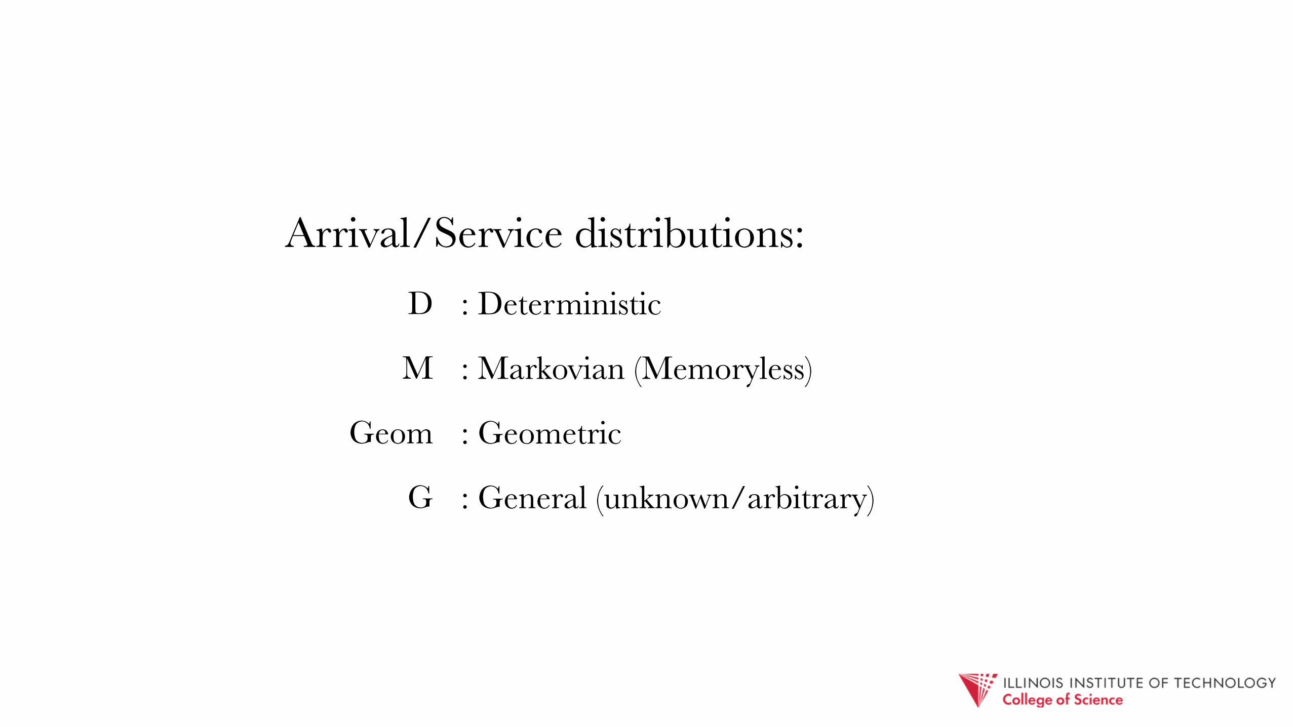
Arrival/Service distributions:D : Deterministic

M : Markovian (Memoryless)

Geom : Geometric

G : General (unknown/arbitrary)

Favorite: Markovian (Exponential)

- combination of multiple independent distributions ⇒ exponential distribution

- when distribution is unknown, exp is a fair compromise: medium variability (CX=1)

- it really simplifies the math!

¶ M/M/1 queueing system

M/M/1 = - Poisson arrival process

- Exponential service times

- 1 server

-∞ buffer length

-∞ population

- FCFS queue discipline

λ μ

i.e., queueing system above with exponential arrival rate λ, exponential service rate μ

L (# of customers in system) can be used to describe the state of the system.

λ and μ are rates of flow between each state

0 1 2 3 ...

λ

μ

λ

μ

λ

μ

λ

μ

model as a Markov chain:

0 1 2 3 ...

λ

μ

λ

μ

λ

μ

λ

μ

is probability of L=n at time t

want the limiting distribution (i.e., at equilibrium):

P (Lt = n)

pn = limt!1

P (Lt = n |L0 = i), i = 0, 1, 2, . . .

0 1 2 3 ...

λ

μ

λ

μ

λ

μ

λ

μ

“balance” equations (apply at equilibrium):

�p0 = µp1

(�+ µ)pn = �pn�1 + µpn+1

1X

n=0

pn = 1

�p0 = µp1

(�+ µ)pn = �pn�1 + µpn+1

0 1 2 3 ...

λ

μ

λ

μ

λ

μ

λ

μ

together with

can derive distribution of L

,

but we will limit ourselves to mean value analysis

P (Lq = 0)

P (Lq � x)

P (T t)

E(Tq), E(T )

E(Lq), E(L)

don’t really need the distributions to compute these mean values …

Big help: PASTA property

“Poisson Arrivals See Time Averages”

i.e., arriving customers in a Poisson process see, on average, the same number of customers in thesystem as predicted by the steady-state average

E(L) = 5 people in store- i.e., to the outside observer, there are 5 people in the store on average

- given Poisson arrivals, new customers on average also see 5 people in the store

not true in general!

consider deterministic system: - arrival times = 1, 3, 5, 7, …

- service time = 1 (constant)

- E(L) = 1/2

but arriving customers always see 0 in store!

E(Tq) = E(Lq)E(Ts) + ⇢E(Tr)

E(Tq)� �E(Tq)E(Ts) = ⇢E(Tr)

E(Tq)(1� �E(Ts)) = ⇢E(Tr)

E(Tq) =⇢E(Tr)

1� �E(Ts)

=⇢E(Tr)

1� ⇢

Start analysis with mean wait time: E(Tq)time for waiting customers ahead of me to be served

E(Tq) =if the server is busy, the residual service time of customer in service

+

= �E(Tq)E(Ts) + ⇢E(Tr)

(by Little’s Law)

Pollaczek-Khinchin formula

E(Tr)?

consider deterministic case: - if mean service time = 1 min, and we arriveto find server occupied, E(Tr) = ? - Ans: 30 sec (E(Ts)/2)

E(Tr)?

what about Poisson arrival process? - by PASTA, new arrivals sees average! - i.e., E(Tr) = E(Ts)

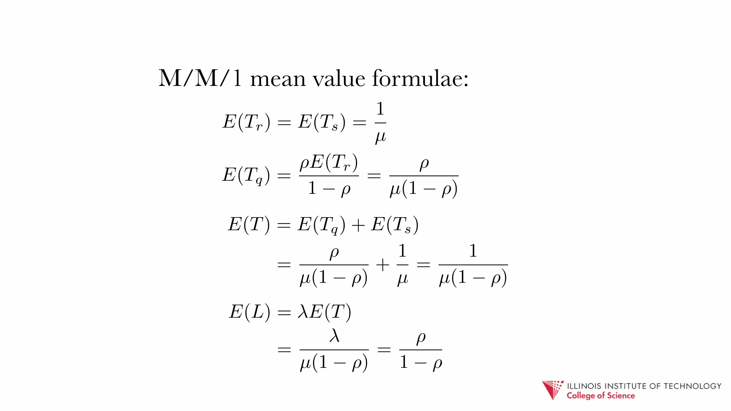
M/M/1 mean value formulae:

E(Tr) = E(Ts) =1

µ

E(Tq) =⇢E(Tr)

1� ⇢=

⇢

µ(1� ⇢)

E(T ) = E(Tq) + E(Ts)

=⇢

µ(1� ⇢)+

1

µ=

1

µ(1� ⇢)

E(L) = �E(T )

=�

µ(1� ⇢)=

⇢

1� ⇢

e.g., Suppose a network server receives 40 requests per second, and the average service time is 20ms. Assuming requests are exponentially distributed:

1.What is the average server utilization?

2.What is the average time spent in the server’s queue?

3.What is the average turnaround time for a request?

E(L) = �E(T )Little’s Law: Mean wait time:

E(Tq) =⇢

µ(1� ⇢)

� = 40/s, E(Ts) = 20ms = 0.02sGiven:

E(Tq) =0.02⇥ 0.8

1� 0.8= 0.08s = 80ms

Mean wait time:

E(T ) = E(Tq) + E(Ts) = 80ms + 20ms = 100msMean sojourn time:

⇢, E(Tq), E(T )Find:

⇢ = �E(Ts) = 40⇥ 0.02 = 0.8Utilization:

e.g., Suppose we upgrade the server and lower mean service time from 20ms to 15ms. By how much does this improve turnaround time? (Arrival rate still = 40/s)

⇢ = 40⇥ 0.015 = 0.6

E(T ) =15ms

1� 0.6= 37.5ms

100� 37.5

100= 62.5% improvement!

20� 15

20= 25% decrease in service time

e.g., A new cafeteria has just opened on campus, and is set up to service, on average, 2 students/minute. Students are only starting to trickle in, but the manager has already decided that when the average time needed for them to get their food approaches 5 minutes, capacity will be increased. Assuming a M/M/1 system:

1. What would the mean arrival rate need to be for the manager to increase capacity?

2. How many students would be waiting for service at this point?

E(T ) =1

µ(1� ⇢)E(L) = �E(T )

Given:Find: �, E(Lq)

µ = 2/min, E(T ) ! 5min

5 =1

µ� �) � = µ� 1

5

E(T ) =1

µ� �

= 1.8/min

E(Tq) = E(T )� E(Ts) = 5� 1

2= 4.5

E(Lq) = �E(Tq) = 1.8⇥ 4.5 = 8.1

e.g., Potbelly's is getting ready to open a new store at the MTCC, and is expecting approximately 8 students to arrive per minute during the lunch rush. If they want to guarantee that no more than 10 students, on average, are waiting in line to get serviced, how quickly must they be able to take and complete orders?

E(L) = �E(T )

Little’s Law: Mean wait time:E(Tq) =

⇢

µ(1� ⇢)

Given: � = 8 E(Lq) 10, wantFind: µ

1.25 =�

µ2(1� ⇢)=

�

µ2 � µ�

µ2 � 8µ� 6.4 = 0

E(Tq) =E(Lq)

�=

10

8= 1.25 =

⇢

µ(1� ⇢)

¶ M/G/1 queueing system

Arbitrary (General) service distribution, but:

- Can assume stable system (ρ<1)

- Little’s Law still applies

- Still have PASTA!

E(Tq) =⇢E(Tr)

1� ⇢

E(Tr) depends on mean and variance of service times

for exponential, C2Ts

= 1, so E(Tr) =1 + 1

2· E(Ts) = E(Ts)

for deterministic, C2Ts

= 0, so E(Tr) =0 + 1

2· E(Ts) =

E(Ts)

2

Intuition:larger variance means that residual time is a bigger fraction of the mean

E(Tr) =�2(Ts) + E(Ts)2

2E(Ts)=

C2Ts

+ 1

2· E(Ts)

e.g., A print shop has 4 clients, each of which sends in a job every half hour on average, distributed exponentially. It takes an average of 6 minutes to print each job (there is one printer), and the service distribution can be described with C2=1.5.

1. How many jobs are, on average, waiting?

2. What is the average job turnaround time?

� = 4⇥ 2/hour = 8/hour

E(Ts) = 6 min = 0.1 hour

E(Tq) =⇢

1� ⇢·C2

Ts+ 1

2· E(Ts)

E(Lq) = �E(Tq) = 8⇥ 0.5 = 4

E(T ) = E(Tq) + E(Ts) = 0.6 hour = 36 min

=0.8

0.2⇥ 2.5

2⇥ 0.1 = 0.5 hour

C2Ts

= 1.5

Given:

⇢ = 8⇥ 0.1 = 0.8

E(Lq), E(T )Find: