
Basic Properties of Slow-Fast Nonlinear Dynamical System ... · Basic Properties of Slow-Fast...
10
Basic Properties of Slow-Fast Nonlinear Dynamical System in the Atmosphere-Ocean Aggregate Modeling SERGEI SOLDATENKO 1 and DENIS CHICHKINE 2 1 Center for Australian Weather and Climate Research Earth System Modeling Research Program 700 Collins Street, Melbourne, VIC 3008 AUSTRALIA [email protected] 2 University of Waterloo Faculty of Mathematics 200 University Avenue West, ON N2L 3G1 CANADA Abstract: Complex dynamical processes occurring in the earth’s climate system are strongly nonlinear and exhibit wave-like oscillations within broad time-space spectrum. One way to imitate essential features of such processes is using a coupled nonlinear dynamical system, obtained by combining two versions of the well- known Lorenz (1963) model with distinct time scales that differ by a certain time-scale factor. This dynamical system is frequently applied for studying various aspects of atmospheric and climate dynamics, as well as for estimating the effectiveness of numerical algorithms and techniques used in numerical weather prediction, data assimilation and climate simulation. This paper examines basic dynamic, correlation and spectral properties of this system, and quantifies the influence of the coupling strength on power spectrum densities, spectrograms and autocorrelation functions. Key-Words: dynamical system, earth’s climate system, numerical weather prediction, spectral properties 1 Introduction Theory of dynamical systems enables us to explore temporal and spatial evolution of the earth’s climate system and its components [1]. The “earth’s climate system” is a term that is used to refer to the interacting atmosphere, hydrosphere, lithosphere, cryosphere, biosphere as well as numerous natural and anthropogenic physical, chemical, and biological cycles of our planet. Each of these components has unique dynamics and physics, and is characterised by specific time-space spectrum of motions, characteristic time, internal variability, and other properties [2]. Dynamical processes occurring in the earth’s climate system have turbulent nature and exhibit wave-like oscillations within broad time-space spectrum, and, therefore, are characterized by strong nonlinearity [3]. In this context, numerical weather prediction (NWP) and climate simulation represent one of the most complex and important applications of dynamical systems theory and its concepts and methods. It is important to emphasize, that NWP and climate simulation focus on processes with very different time scales and, in more importantly, pursue very different objectives [4, 5]. NWP is a typical initial value problem aiming to predict, as precisely as possible, the future state of the atmosphere taking into account current (initial) weather conditions. To date, due to the intrinsic limits with regards to the predictability of atmospheric processes, the practical importance of NWP is limited to a time horizon of 7 – 10 days. Errors in the NWP are primarily generated by inaccuracies in the initial conditions rather than by the imperfections in mathematical models [6]. By contrast, climate change and variability simulations focus on much longer time scales (several months or even years) and involve the study of stability of climate model attractors with respect to external forcing. Despite these fundamental differences, deterministic mathematical models, based on the same physical principles and fundamental laws of physics such as conservation of momentum, energy and mass, are commonly applied to both NWP and climate simulations. Mathematically, these physical laws and principles are generally expressed in terms of a set of nonlinear partial differential equations (PDEs) and, in their discrete form, contain a large number of state variables and parameters. WSEAS TRANSACTIONS on SYSTEMS Sergei Soldatenko, Denis Chichkine E-ISSN: 2224-2678 757 Volume 13, 2014
-
Upload
nguyenkiet -
Category
Documents
-
view
215 -
download
0
Transcript of Basic Properties of Slow-Fast Nonlinear Dynamical System ... · Basic Properties of Slow-Fast...

Basic Properties of Slow-Fast Nonlinear Dynamical System in the
Atmosphere-Ocean Aggregate Modeling
SERGEI SOLDATENKO1 and DENIS CHICHKINE
2
1Center for Australian Weather and Climate Research
Earth System Modeling Research Program
700 Collins Street, Melbourne, VIC 3008
AUSTRALIA
[email protected] 2University of Waterloo
Faculty of Mathematics
200 University Avenue West, ON N2L 3G1
CANADA
Abstract: Complex dynamical processes occurring in the earth’s climate system are strongly nonlinear and
exhibit wave-like oscillations within broad time-space spectrum. One way to imitate essential features of such
processes is using a coupled nonlinear dynamical system, obtained by combining two versions of the well-
known Lorenz (1963) model with distinct time scales that differ by a certain time-scale factor. This dynamical
system is frequently applied for studying various aspects of atmospheric and climate dynamics, as well as for
estimating the effectiveness of numerical algorithms and techniques used in numerical weather prediction, data
assimilation and climate simulation. This paper examines basic dynamic, correlation and spectral properties of
this system, and quantifies the influence of the coupling strength on power spectrum densities, spectrograms
and autocorrelation functions.
Key-Words: dynamical system, earth’s climate system, numerical weather prediction, spectral properties
1 Introduction Theory of dynamical systems enables us to explore
temporal and spatial evolution of the earth’s climate
system and its components [1]. The “earth’s climate
system” is a term that is used to refer to the
interacting atmosphere, hydrosphere, lithosphere,
cryosphere, biosphere as well as numerous natural
and anthropogenic physical, chemical, and
biological cycles of our planet. Each of these
components has unique dynamics and physics, and
is characterised by specific time-space spectrum of
motions, characteristic time, internal variability, and
other properties [2].
Dynamical processes occurring in the earth’s
climate system have turbulent nature and exhibit
wave-like oscillations within broad time-space
spectrum, and, therefore, are characterized by strong
nonlinearity [3]. In this context, numerical weather
prediction (NWP) and climate simulation represent
one of the most complex and important applications
of dynamical systems theory and its concepts and
methods.
It is important to emphasize, that NWP and
climate simulation focus on processes with very
different time scales and, in more importantly,
pursue very different objectives [4, 5]. NWP is a
typical initial value problem aiming to predict, as
precisely as possible, the future state of the
atmosphere taking into account current (initial)
weather conditions. To date, due to the intrinsic
limits with regards to the predictability of
atmospheric processes, the practical importance of
NWP is limited to a time horizon of 7 – 10 days.
Errors in the NWP are primarily generated by
inaccuracies in the initial conditions rather than by
the imperfections in mathematical models [6]. By
contrast, climate change and variability simulations
focus on much longer time scales (several months or
even years) and involve the study of stability of
climate model attractors with respect to external
forcing. Despite these fundamental differences,
deterministic mathematical models, based on the
same physical principles and fundamental laws of
physics such as conservation of momentum, energy
and mass, are commonly applied to both NWP and
climate simulations. Mathematically, these physical
laws and principles are generally expressed in terms
of a set of nonlinear partial differential equations
(PDEs) and, in their discrete form, contain a large
number of state variables and parameters.
WSEAS TRANSACTIONS on SYSTEMS Sergei Soldatenko, Denis Chichkine
E-ISSN: 2224-2678 757 Volume 13, 2014
Performing a detailed simulation of the dynamics of
the earth’s climate system and its components using
such models requires significant computational
resources and considerable time for analysis and
interpretation of obtained results. Consequently,
low-order models have drawn attention of scientists
as very compact and convenient tools for studying
various aspects of dynamics of natural physical
processes and phenomena, and also for estimating
the effectiveness of numerical algorithms and
techniques used in computational simulations.
To simulate and predict the behavior and
changes in the earth’s climate system, integrated
models that link together models of the atmosphere,
oceans, sea-ice, land surface, biochemical cycles
including those of carbon and nitrogen, chemistry
and aerosols are required. In environmental,
geophysical and engineering sciences one of the
most widely used low-order systems is a coupled
system obtained by combining of several versions of
the well-known original Lorenz system [7]
(hereinafter referred to as the L63 system) with
distinct time scales differing by a certain time-scale
factor. Coupling of two systems, one with “fast” and
another with “slow” time scales, allows imitating
the interaction between a fast-oscillating atmosphere
and slow-fluctuating ocean. This coupled system
was successfully applied to climate studies (e.g. [8,
9]), numerical weather prediction and data
assimilation (e.g. [10-12]), sensitivity analysis,
parameter estimations and predictability studies
(e.g. [13 – 16]). The coupled Lorenz system, in spite
of its simplicity, is capable of simulating some
essential properties of the general circulation of the
atmosphere and ocean and allows, with negligible
computational costs, to obtain realistic and
reasonable qualitative and quantitative results, while
retaining the essential physics. The correct
application of this system requires knowledge of its
dynamics, spectral and other properties.
This paper will look at the basic properties of a
coupled chaotic nonlinear system obtained by
combining “fast” and “slow” versions of the L63
system, corresponding to time scales of the NWP
and climate variability simulations respectively.
2 Coupled Dynamical System
2.1 Dynamical system concept In the most general sense, an abstract dynamical
system can be formally specified by its state vector
the coordinates of which (state or dynamic
variables) characterize exactly the state of a system
at any moment, and a well-defined function (i.e.
rule) which describes, given the current state, the
evolution with time of state variables. There are two
kinds of dynamical system: continuous time and
discrete time. Continuous-time dynamical systems
are commonly specified by a set of ordinary or
partial differential equations and the problem of the
evolution of state variables in time is then
considered as an initial value problem. With
respect to the earth system simulations, discrete-
time deterministic systems are of particular interest,
because, in a general case, the solution of
differential equations describing the evolution of the
earth’s climate system and its subsystems can be
only obtained numerically.
Let the current state of an abstract dynamical
system is defined by the following set of n real
variables u1, u2,…,un. The number n is referred as
the dimension of the system. A particular state u =
(u1, u2,…,un) corresponds to a point in an n-
dimensional space Un , the so-called phase
space of the system. Let tm ( 0,1,2,m ) be
the discrete time, and f = (f1, f2,…,fn) is a smooth
vector-valued function defined in the domain nU . The function f describes the evolution of
the system state from the moment of time t0=0 to the
state of the system at the moment of time mt such
that f: U→U. Thus, a deterministic dynamical
system with discrete time can be specified by the
following equations:
1 0 0, m mu t f u t u t u , (1)
m=0, 1, 2, … .
The sequence 0m m
u t
is a trajectory of the
system (1) in its phase space u U , which is
uniquely defined by the initial values of state
variables u0 (initial conditions):
0
m
mu t f u , (2)
where 0
mf u denotes a m-fold application of f
to u0.
In relation to modeling of the earth’s climate
system, the vector-function f is a nonlinear function
of the state variables. Nonlinearity can arise from
the numerous feedbacks existed between the
different components of the system, external forcing
caused by natural and anthropogenic processes and
the chaotic nature of dynamical processes occurring
in geospheres.
WSEAS TRANSACTIONS on SYSTEMS Sergei Soldatenko, Denis Chichkine
E-ISSN: 2224-2678 758 Volume 13, 2014

2.2 Coupled nonlinear dynamical system A multiscale nonlinear dynamical system examined
in this paper is derived by coupling the fast and slow
versions of the original L63 system [7] and can be
written as follows [17, 18]:
a) the fast subsystem
,x y x c aX k
( ),y rx y xz c aY k
,zz xy bz c Z
b) the slow subsystem
,
( ) ( ),
( ) ,z
X Y X c x k
Y rX Y aXZ c y k
Z aXY bZ c z
where lower case letters x, y and z represent the
dynamic variables of the fast model, capital letters
X, Y and Z denote the state variables of the slow
model, ζ>0, r>0 and b>0 are the parameters of the
original L63 model, ε is a time-scale factor (if, for
instance, ε =0.1 then the slow subsystem is ten times
slower than the fast subsystem), c is a coupling
strength for x, X, y and Y variables, cz is a coupling
strength parameter for z and Z variables, k is a
“decentring” parameter [17], and a is a parameter
representing the amplitude scale factor (for instance,
a=1 indicates that slow and fast subsystems have the
same amplitude scale). The coupling strength
parameters c and cz control the interconnection
between fast and slow subsystems: the smaller the
parameters c and cz, the weaker the interdependence
between two subsystems. Without loss of generality,
one can assume that a=1, k=0 and c=cz, then
equations of the model can be represented in an
operator form as follows
; du
A u p udt
, (3)
where u=(x,y,z,X,Y,Z)T is a model state vector,
p=(ζ,b,r,ε,c)T is a vector of model parameters, and
A(u; p) is the matrix operator such that
0 0 0
1 0 0
0 0 0
0 0 0
0 0
0 0 0
c
r x c
x b cA
c
c r X
c Y b
Thus, system of autonomous ODEs (3) has five
control parameters (ζ, r, b, c and ε) and together
with given initial conditions u(t0)=u0 represents an
initial value problem.
2.3 Equations in variational form Equations in variational form are used to study the
system’s dynamical properties. These equations can
be obtained by linearization of (3) around a certain
trajectory, which is a particular solution of (3) and
represents a vector-function ( )u t , t[0,∞). Assume
that the system (6) operates along the trajectory u*(t)
and let δu(t) be an infinitesimal perturbation of the
state vector, i.e. δu(t) = u(t) - u*(t). Approximating
the right-hand side of (6) by a Taylor expansion in
the vicinity of u*(t) and neglecting 2
nd order and
higher order terms, one can obtain the following set
of linear ODEs, the equations in variations:
0 0
( ),
d u tJ u t u t u
dt
, (4)
where *u u
AJ
u
is a Jacobean matrix:
0 0 0
1 0 0
0 0
0 0 0
0 0
0 0
c
r z x c
y x b cJ
c
c r Z X
c Y X b
Variational equations (4) can be rewritten as
0 0 0( ) , tu t L u u t u , (5)
where Lt is a linear solution operator.
2.4 Model parameters The time evolution of coupled nonlinear system (3)
is conditioned by a set of ODEs and control
parameters ζ, r, b, c and ε. By setting parameter c
equal to zero, one can restore the original L63
model. Standard values of the L63 parameters
corresponding to chaotic behaviour are:
10, 8 3,b and 28r [7]. These parameters
are used in this study since the motions in the
atmosphere and ocean are inherently chaotic. It is
important to note, that for 10 and 8 3b there
is a critical value for parameter r, equal to 24.74,
and any r larger than 24.74 induces chaotic
behaviour of the L63 system [19]. The time scale
factor ε is taken to be 0.1. Thus, in our study, the
main control parameter is the coupling strength c,
which essentially determines the strength of
WSEAS TRANSACTIONS on SYSTEMS Sergei Soldatenko, Denis Chichkine
E-ISSN: 2224-2678 759 Volume 13, 2014
interactions between fast and slow models and,
therefore, the behaviour of the entire coupled
system. In numerical experiments values of this
parameter have been chosen in accordance with [17,
18]: 0.15, 1.0с .
2.5 Numerical integration procedure The system of equations (3) is numerically
integrated by applying a fourth order Runge-Kutta
algorithm with a time step 0.01t . To begin with,
equations (3) are transformed into a discrete-time
form and then integrated. This integration produces
time-series for each of the dynamic variables at
equally-spaced time-points starting from 0t , denoted
by
, , 0, , 1m m mu u t t m t m M ,
where t is the integration time step, also known as
the sampling interval. To discard the initial transient
period the numerical integration starts at time 142Tt t with the initial conditions
0.01; 0.01; 0.01; 0.02; 0.02; 0.02Tu
(6)
and finishes at time 0t . In addition, this ensures that
the calculated vector of dynamic variables u0=u(t0)
is on the system’s attractor. The state vector u0 is
then used as the initial conditions for further
numerical experiments. Note that, for 0.01t , the
numerical integration with length of 100 time steps
corresponds to one non-dimensional unit of time.
3 Coupled System Properties
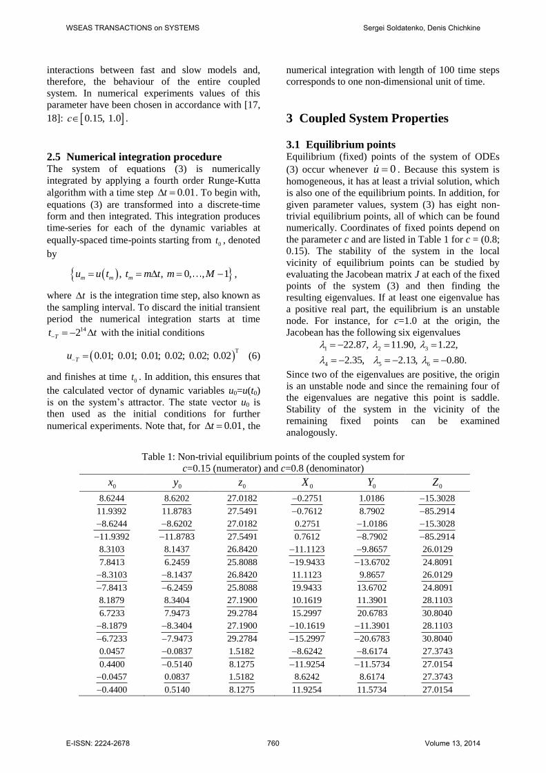
3.1 Equilibrium points Equilibrium (fixed) points of the system of ODEs
(3) occur whenever 0u . Because this system is
homogeneous, it has at least a trivial solution, which
is also one of the equilibrium points. In addition, for
given parameter values, system (3) has eight non-
trivial equilibrium points, all of which can be found
numerically. Coordinates of fixed points depend on
the parameter c and are listed in Table 1 for c = (0.8;
0.15). The stability of the system in the local
vicinity of equilibrium points can be studied by
evaluating the Jacobean matrix J at each of the fixed
points of the system (3) and then finding the
resulting eigenvalues. If at least one eigenvalue has
a positive real part, the equilibrium is an unstable
node. For instance, for c=1.0 at the origin, the
Jacobean has the following six eigenvalues
1 2 3
4 5 6
22.87, 11.90, 1.22,
2.35, 2.13, 0.80.
Since two of the eigenvalues are positive, the origin
is an unstable node and since the remaining four of
the eigenvalues are negative this point is saddle.
Stability of the system in the vicinity of the
remaining fixed points can be examined
analogously.
Table 1: Non-trivial equilibrium points of the coupled system for
c=0.15 (numerator) and c=0.8 (denominator)
0x 0y 0z 0X 0Y 0Z
8.6244
11.9392
8.6202
11.8783
27.0182
27.5491
0.2751
0.7612
1.0186
8.7902
15.3028
85.2914
8.6244
11.9392
8.6202
11.8783
27.0182
27.5491
0.2751
0.7612
1.0186
8.7902
15.3028
85.2914
8.3103
7.8413
8.1437
6.2459
26.8420
25.8088
11.1123
19.9433
9.8657
13.6702
26.0129
24.8091
8.3103
7.8413
8.1437
6.2459
26.8420
25.8088 11.1123
19.9433 9.8657
13.6702 26.0129
24.8091
8.1879
6.7233 8.3404
7.9473 27.1900
29.2784 10.1619
15.2997 11.3901
20.6783 28.1103
30.8040
8.1879
6.7233
8.3404
7.9473
27.1900
29.2784 10.1619
15.2997
11.3901
20.6783
28.1103
30.8040
0.0457
0.4400 0.0837
0.5140
1.5182
8.1275 8.6242
11.9254
8.6174
11.5734
27.3743
27.0154
0.0457
0.4400
0.0837
0.5140 1.5182
8.1275 8.6242
11.9254 8.6174
11.5734 27.3743
27.0154
WSEAS TRANSACTIONS on SYSTEMS Sergei Soldatenko, Denis Chichkine
E-ISSN: 2224-2678 760 Volume 13, 2014

3.2 Dissipativity Let V be the volume of some region of phase space.
The rate of volume contraction is given by Lie
derivative,
1
1 1 0.
dV x y z X Y Z
V dt x y z X Y Z
b
.
Since the rate of volume contraction is always
negative under the chosen model parameters, the
coupled system (3) is dissipative and, therefore,
volumes in phase space shrink exponentially with
time. This is represented mathematically by
0
tV t V t e .
3.3 Symmetry and invariance One can easily to show that the coupled system (3)
remains invariant under the transformation
: ( , , , , , ) , , , , ,F x y z X Y Z x y z X Y Z .
This means that if
( ), ( ), ( ), ( ), ( ), ( )x t y t z t X t Y t Z t
is a solution of (3), then
( ), ( ), ( ), ( ), ( ), ( )x t y t z t X t Y t Z t
is also a solution. The invariance of z and Z axes
indicates that all trajectories on the z and Z axes
remain on these axes and approach the origin.
Indeed, if
0 0 0 0 0 0 0 0, , , , , 0,0, ,0,0, ,x y z X Y Z z Z
then the model equations are as follows
z bz cZ , (7)
Z bZ cz . (8)
Differentiating equation (7) with respect to t and
then substituting equation (8) into the result of
differentiation gives the following second order
ODE
2 21 0z b z c b z .
This equation is a dumped harmonic oscillator
which can be rewritten as
2
02 0z z z , (9)
where 1 2b is a damping constant, and
2 2 2
0 c b is a natural frequency.
Equation (9) is a linear homogeneous ODE and
its general solution depends on the relationship
between damping constant γ and natural frequency
ω0.
In our example a damping constant 1.47
and the natural frequency 0 depends on the
coupling strength parameter c (Table 2). Critical
frequency 0
c , at which 0 , occurs when
1.2c . Since for our experiments 0.15; 1.0c ,
oscillator (10) is over-dumped (0 ) and its
general solution is given by the following equation
1 2t tz t Ae Be , (10)
where 2
1,2 0 0 1 , and A, B are
unknown constants of integration. The solution of
equation (10) asymptotically tends to the
equilibrium z=Z=0 without oscillations: as t ,
the dynamic variables z and Z tend to zero.
Table 2: Natural frequency 0 for different values of the coupling strength parameter
c 0.01 0.15 0.5 0.8 1.0 1.2 1.5
0 0.8422 0.8565 0.9804 1.1624 1.3081 1.4667 1.7208
3.4 System attractor The structure of the resulting attractor depends on
the coupling strength parameter c. Figs. 1 and 2
illustrate phase portraits in x–y, x–z, and y–z phase
planes of both fast and slow subsystems for weak
(c=0.15) and strong (c=0.8) coupling, respectively.
It is known, that the L63 model produces chaotic
oscillations of a switching type: the structure of its
attractor contains two regions divided by the stabile
manifold of a saddle point in the origin. For
relatively small coupling strength parameter (c<0.5),
the attractor for both fast and slow subsystems
maintains a chaotic structure, which is inherent in
the original L63 attractor. As the parameter c
increases, the attractor for both fast and slow sub-
systems undergoes structural changes breaking the
patterns of the original L63 attractor.
WSEAS TRANSACTIONS on SYSTEMS Sergei Soldatenko, Denis Chichkine
E-ISSN: 2224-2678 761 Volume 13, 2014

Fig. 1: Phase portraits for fast and slow subsystem
for c=0.15.
Fast and slow subsystems affect each other
through coupling terms, and at some value of the
coupling strength parameter ( 0.5c ) a chaotic
behavior is destroyed and dynamic variables begin
to exhibit some sophisticated motions which are not
obviously periodic. Moreover, qualitative
examination shows that the evolution through time
of both subsystems becomes, to large degree,
synchronous (however, phase synchronization
requires specific analysis which is not within the
scope of this paper). For example, for c=0.8 the
plane phase portraits X – Y, X – Z and Y – Z of the
slow subsystem represent closed curves which are
mostly smooth and have no visible kinks. These
portraits indicate that the motion possesses periodic
properties. At the same time, the attractor of the
slow subsystem for c=0.8 has a more complex
structure.
3.4 Correlation properties Numerical integration of equations (3) produces the
time series of dynamic variables hereinafter referred
to as signals or oscillations. We can conduct the
diagnosis of the coupled dynamical system by
analysing the signals using standard tools such as
autocorrelation functions and the distribution of
power density in the frequency domain from signals
obtained in the time domain.
Autocorrelation functions (ACFs) enable one to
distinguish between regular and chaotic processes
and to detect transition from order to chaos. In
particular, for chaotic motions, ACF decreases in
Fig. 2: Phase portraits for fast and slow subsystem
for c=0.8.
time, in many cases exponentially, while for regular
motions, ACF is unchanged or oscillating. In
general, however, the behaviour of ACFs of chaotic
oscillations is frequently very complicated and
depends on many factors (e.g. [20, 21]).
Autocorrelation functions can also be used to define
the so-called typical time memory (typical
timescale) of a process [22]. If it is positive, ACF is
considered to have some degree of persistence: a
tendency for a system to remain in the same state
from one moment in time to the next. The ACF for a
given discrete dynamic variable 1
0
M
m mu
is defined
as
m m s m m sC s u u u u ,
where the angular brackets denote ensemble
averaging. Assuming time series originates from a
stationary and ergodic process, ensemble averaging
can be replaced by time averaging over a single
normal realization
2
m m sC s u u u .
Signal analysis commonly uses the normalized
ACF, defined as 0R s C s C .
ACF plots for realizations of dynamic variables x
and X, and z and Z calculated for different values of
the coupling strength parameter c are presented in
Figs. 3 and 4, respectively. For relatively small
parameter c ( 0.4c ), the ACFs for both x and X
variables decrease fairly rapidly to zero, consistently
with the chaotic behaviour of the coupled system.
WSEAS TRANSACTIONS on SYSTEMS Sergei Soldatenko, Denis Chichkine
E-ISSN: 2224-2678 762 Volume 13, 2014

Fig. 3: Autocorrelation functions for dynamic
variables x and X for different parameter c.
However, as expected, the rate of decay of the ACF
of the slow variable X is less than that of the fast
variable x.
The ACFs for variables z and Z (really, their
envelopes) also decay almost exponentially from the
maximum to zero. For coupling strength parameter
on the interval 0.4 0.6c the ACF of the fast
variable x becomes smooth and converges to zero.
At the same time, the envelopes of the ACFs of
variables X, z and Z demonstrate a fairly rapid fall,
indicating the chaotic behaviour. As the parameter c
increases, the ACFs become periodic and their
envelopes decay slowly with time, indicating
transition to regularity. For 0.8c calculated
ACFs show periodic signal components.
3.5 Spectral properties
For a given discrete-time signal 1
0
M
m mu
the power
spectrum density (PSD) characterizes the signal
intensity (power) per unit of bandwidth. For a wide-
sense stationary process, the Wiener-Khinchin
theorem relates the ACF to the PSD by means of a
Fourier transform (i.e. PSD is a Fourier transform of
ACF) and provides information about correlation
structure of the time series generated by the system.
Fig. 4: Autocorrelation functions for dynamic
variables z and Z for different parameter c.
The term “power spectral density function” is
frequently shortened to spectrum. The units of PSD
are u2/Hz, irrespective of what the units of u are.
Oscillations of different types have specific spectral
properties and, therefore, can be characterized by
their PSD. For instance, a periodic motion
consisting of the sum of finite number of sine curves
has a set of lines in its spectrum, whereas a chaotic
motion has a continuous spectral density function.
Fig. 5: PSD estimates of fast (x and z) and slow
(X and Z) dynamic variables for c=0.15.
WSEAS TRANSACTIONS on SYSTEMS Sergei Soldatenko, Denis Chichkine
E-ISSN: 2224-2678 763 Volume 13, 2014

Fig. 6: PSD estimates of fast (x and z) and slow (X
and Z) dynamic variables for c=0.8.
Generally, the ACF and spectrum represent
different characterization of the same time series
information. However, the ACF analyzes
information in the time domain, and the spectrum in
the frequency domain.
There are several methods, both parametric and
nonparametric, for spectrum estimation [23, 24].
This paper uses periodogram, which is the most
common nonparametric method for computing the
PSD estimate of time series. This method calculates
PSD based on the discrete Fourier transform (DFT).
Let’s define the DFT of sequence 1
0
M
m mu
as
1
2
0
, 0, , 1M
i M mk
k m
m
U u e k M
,
where k is a discrete normalized frequency. Then
the spectrum can be represented as follows
2
, 0, , 1k
k
s
UP k M
Mf .
The spectrum Pk can be plotted on a dB scale,
relative to the reference amplitude Pref =1, therefore
1010 log , 0, , 1dB
k kP P k M .
The frequency fk corresponding to point k of the
DFT is
sk
ff k
M
The PSD estimates for fast (x and z) and slow (X
and Z) variables as well as for weak (c=0.15) and
strong (c=0.8) coupling are shown in Figs. 5 and 6,
respectively. For weak coupling, the signal power
for all dynamic variables decreases exponentially
from low frequencies toward higher frequencies and
distinctive energy peaks are not present for almost
all variables. The only exception is the fast variable
z, for which a local peak is observed at frequency
~1.2 Hz. For weak coupling, the spectrum of the fast
subsystem is similar to the spectrum of the L63
model: the fast subsystem generates a broadband
spectrum reminiscent of random noise
corresponding to irregular aperiodic oscillations. At
the same time, the low-frequency component
strongly dominates in the spectrum of slow
subsystem. As the coupling strength increases, the
power spectrum of both fast and slow subsystems
shifts toward the low frequencies, which
predominate in the spectra.
Fig. 7: Spectrogram for fast and slow dynamic
variables for c=0.15.
Spectrogram is another powerful technique used
in many applications for estimating the spectrum of the time series data. Spectrogram provides information about power as a function of frequency and time, and is generally presented as plot with the frequency of the signal shown on the vertical axis, time on the horizontal axis, and signal power on a colour-scale. Thus, for a given time frame the spectrogram provides the information about frequency content of a signal. Normalized
WSEAS TRANSACTIONS on SYSTEMS Sergei Soldatenko, Denis Chichkine
E-ISSN: 2224-2678 764 Volume 13, 2014

spectrograms for fast (x, y and z) and slow (X, Y and Z) variables for weak (c=0.15) and strong (c=0.8) coupling are shown in Figs. 7 and 8, respectively, with red color representing the highest signal power and blue the lowest. Calculated spectrograms are fully consistent with the PSPs, providing additional information about dominant and minor frequencies in the spectrum for a given time.
Fig. 8: Spectrogram for fast and slow dynamic
variables for c=0.8.
4 Conclusion The low-order coupled chaotic dynamical system
discussed in this paper represents a powerful tool to
study various physical and computational aspects of
numerical weather prediction, data assimilation and
climate simulation. However, the NWP and climate
modeling pursue very different objectives and are
focused on dynamical processes of significantly
different spatial and time scales.
The integration time η of the system equations
can be classified based on its duration as short,
intermediate, long and very long [14], with the
corresponding values of η set to η = 0.1, η = 0.44, η
= 2.26 and η = 131.36, respectively. The short
integration times traverse some portion of a
trajectory along the attractor, the intermediate
integrations correspond to complete circle around
the attractor, the long integrations complete several
circles, and the very long integrations correspond to
movement along the attractor of about 100 times.
The time step Δt=0.01 used in the numerical
integrations is equivalent to 1.2 hours of a real time
[7]. Therefore, intermediate and long-time intervals
defined above correspond to 2.2 and 11.3 days,
respectively, which are consistent with the NWP
and data assimilation time of integrations. In turn,
the very long integration intervals correspond to
climate modeling time scales.
This paper analysed the basic dynamical,
correlation and spectral properties of the nonlinear
chaotic coupled dynamical system consisting of two
versions of the L63 model. The autocorrelation
functions, power spectrum densities and
spectrograms for dynamic variables of the fast and
slow subsystems were computed by numerical
integration of the system equations. The influence of
the coupling strength parameter on the ACFs, PSDs
and spectrograms of system’s dynamic variables
was estimated.
By changing the coupling strength parameter
c, one can obtain the system behaviour that
reflects the major dynamical patterns of weather
and climate for given natural conditions. The
results of this paper can be applied to study
multiscale chaotic dynamical processes occurring in
complex technical systems, nature and society.
References:
[1] H.A. Dijkstra, Nonlinear climate dynamics,
Cambridge University Press, New York, 2013.
[2] J. Marshall and R.A. Plumb, Atmosphere,
ocean and climate dynamics, Academic Press,
San Diego, 2007.
[3] J. Pedlosky, Waves in the ocean and
atmosphere, Springer-Verlag, Berlin, 2nd
edition, 2003.
[4] E. Kalnay, Atmospheric modelling, data
assimilation and predictability, Cambridge
University Press, Cambridge, 2003.
[5] T.T. Warner, Numerical weather and climate
prediction, Cambridge University Press,
Cambridge, 2011.
[6] F. Rabier, E. Klinker, P. Courtier, and A.
Hollingsworth, Sensitivity of forecast to initial
conditions, Quarterly Journal of the Royal
Meteorological Society, Vol. 122, 1996, pp.
121-150. [7] E.N. Lorenz, Deterministic non-periodic flow,
Journal of the Atmospheric Sciences, Vol. 20,
WSEAS TRANSACTIONS on SYSTEMS Sergei Soldatenko, Denis Chichkine
E-ISSN: 2224-2678 765 Volume 13, 2014

1963, pp. 130-141.
[8] T.N. Palmer, Extended-range atmospheric
prediction and the Lorenz model, Bulletin of
the American Meteorological Society, Vol. 74,
1993, pp. 49-66.
[9] P.J. Roeber, Climate variability in a low-order
coupled atmosphere-ocean model, Tellus, Vol.
47A, 1995, pp. 473-494.
[10] P. Gaurtier, Chaos and quadric-dimensional
data assimilation: a study based on the Lorenz
model, Tellus, Vol. 44 A, 1992, pp. 2-17.
[11] G. Evensen, Inverse methods and data
assimilation in non-linear ocean models,
Physica D, Vol. 77, 1994, pp. 108-129.
[12] R.N. Miller, M. Ghil, and F. Gauthiez,
Advanced data assimilation in strongly non-
linear dynamical systems, Journal of the
Atmospheric Sciences, Vol. 51, 1994, pp. 1037-
1056.
[13] L.A Smith, C. Ziehmann and K. Fraedrich,
Uncertainty dynamics and predictability in
chaotic systems, Quarterly Journal of the
Royal Meteorological Society, Vol. 125, 1999,
pp. 2855-2886.
[14] D.J. Lea, M.R. Allen, and T.W.N. Haine,
Sensitivity analysis of the climate of a chaotic
system, Tellus, Vol. 52A, 2000, pp. 523–532.
[15] J.D. Annan and J.C. Hargreaves, Efficient
parameter estimation for a highly chaotic
system, Tellus, Vol. 56 A, 2004, pp. 520-526.
[16] S. Soldatenko, D. Smith, P. Steinle and C.
Tingwell, Sensitivity of coupled chaotic
dynamical system to parameters in the context
of data assimilation, Journal of Mathematics
and System Science, Vol. 3, 2013, pp. 641-654.
[17] M. Peña and E. Kalnay, Separating fast and
slow modes in coupled chaotic systems,
Nonlinear Processes in Geophysics, Vol 11,
2004, pp. 319-327.
[18] L. Siquera and B. Kirtman, Predictability of a
low-order interactive ensemble, Nonlinear
Processes in Geophysics, Vol 19, 2012, pp.
273-282.
[19] C.Sparrow, The Lorenz equations: bifurcations,
chaos, and strange attractors, Springer-Verlag,
New York, 1982.
[20] F. Christiansen, G. Paladin, and H.H. Rugh,
Determination of correlation spectra in chaotic
systems, Physical Review Letters, Vol. 65,
1990, pp. 2087-2090.
[21] C. Liverani, Decay of correlations, Annals of
Mathematics, Vol. 142, 1995, pp. 239-301.
[22] S. Panchev and T. Spassova, Simple general
circulation and climate models with memory,
Advances in Atmospheric Sciences, Vol. 22,
2005, pp. 765-769.
[23] A.V. Oppenheimer and R.W. Schafer,
Discrete-time signal processing, Prentice Hall,
3rd edition, 2000.
[24] R.D. Hippenstiel, Detection theory: Applica-
tions and digital signal processing, CRC Press,
Boca Raton, 2002.
WSEAS TRANSACTIONS on SYSTEMS Sergei Soldatenko, Denis Chichkine
E-ISSN: 2224-2678 766 Volume 13, 2014


![Nonlinear dynamical triggering of slow slip on simulated ...cjm38/papers_talks/JohnsonetalJGRDynTriggering2012.pdf[1] Among the most fascinating, recent discoveries in seismology are](https://static.fdocuments.net/doc/165x107/5f7b173393c8d56b592fa384/nonlinear-dynamical-triggering-of-slow-slip-on-simulated-cjm38paperstalksjohnsonetal.jpg)


