Basic notions of quantum information

2Basic notions of quantum information

This chapter introduces the most basic objects and notions of quantuminformation theory, including registers, states, channels, and measurements,and investigates some of their elementary properties.

2.1 Registers and statesThis first section of the chapter concerns registers and states. A register isan abstraction of a physical device in which quantum information may bestored, and the state of a register represents a description of its contents ata particular instant.

2.1.1 Registers and classical state setsThe term register is intended to be suggestive of a computer component inwhich some finite amount of data can be stored and manipulated. While thisis a reasonable picture to keep in mind, it should be understood that anyphysical system in which a finite amount of data may be stored, and whosestate may change over time, could be modeled as a register. For example,a register could represent a medium used to transmit information from asender to a receiver. At an intuitive level, what is most important is thatregisters represent mathematical abstractions of physical objects, or partsof physical objects, that store information.

Definition of registersThe following formal definition of a register is intended to capture a basicbut nevertheless important idea, which is that multiple registers may beviewed collectively as forming a single register. It is natural to choose aninductive definition for this reason.

2.1 Registers and states 59

X

1, 2, 3, 4Y0 Y1

0, 1 0, 1 0, 1

Z1 Z2 Z3

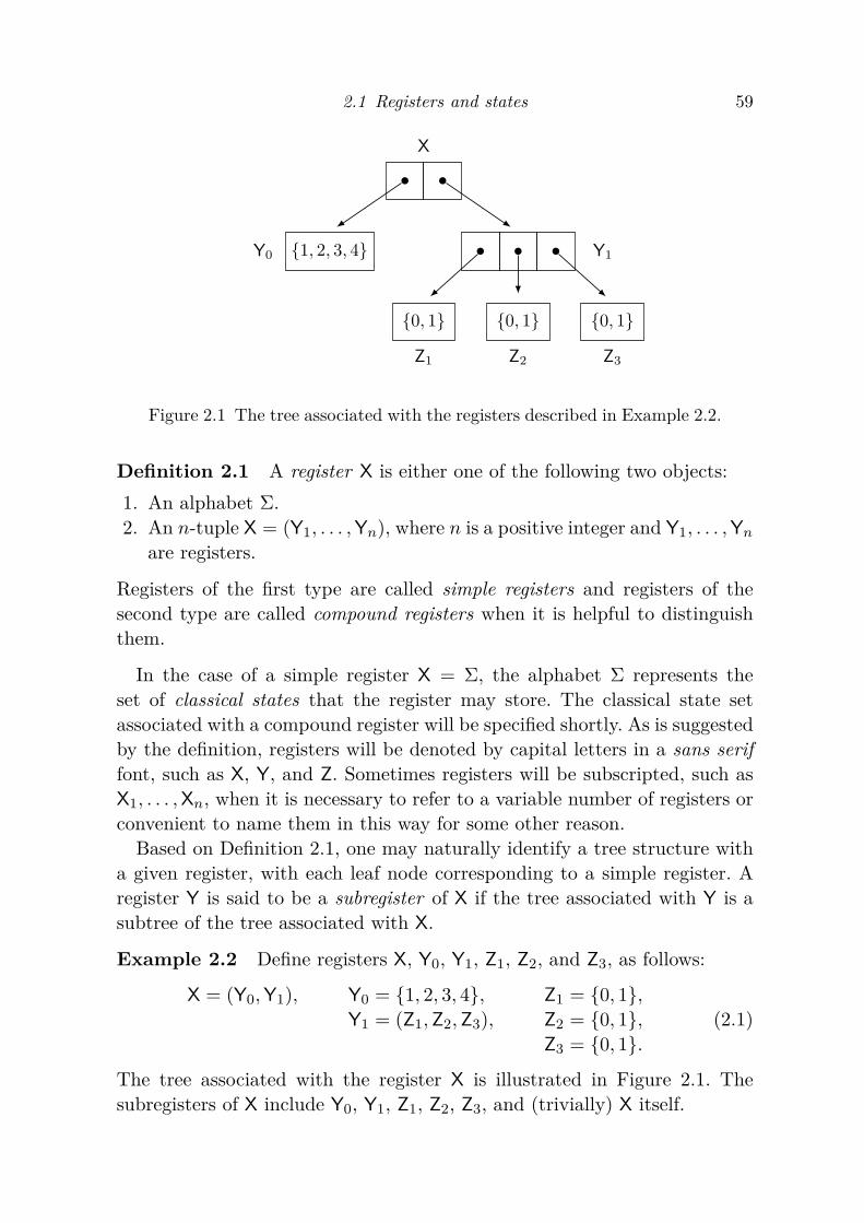
Figure 2.1 The tree associated with the registers described in Example 2.2.

Definition 2.1 A register X is either one of the following two objects:1. An alphabet Σ.2. An n-tuple X = (Y1, . . . ,Yn), where n is a positive integer and Y1, . . . ,Yn

are registers.

Registers of the first type are called simple registers and registers of thesecond type are called compound registers when it is helpful to distinguishthem.

In the case of a simple register X = Σ, the alphabet Σ represents theset of classical states that the register may store. The classical state setassociated with a compound register will be specified shortly. As is suggestedby the definition, registers will be denoted by capital letters in a sans seriffont, such as X, Y, and Z. Sometimes registers will be subscripted, such asX1, . . . ,Xn, when it is necessary to refer to a variable number of registers orconvenient to name them in this way for some other reason.

Based on Definition 2.1, one may naturally identify a tree structure witha given register, with each leaf node corresponding to a simple register. Aregister Y is said to be a subregister of X if the tree associated with Y is asubtree of the tree associated with X.

Example 2.2 Define registers X, Y0, Y1, Z1, Z2, and Z3, as follows:

X = (Y0,Y1), Y0 = 1, 2, 3, 4, Z1 = 0, 1,Y1 = (Z1,Z2,Z3), Z2 = 0, 1,

Z3 = 0, 1.(2.1)

The tree associated with the register X is illustrated in Figure 2.1. Thesubregisters of X include Y0, Y1, Z1, Z2, Z3, and (trivially) X itself.

60 Basic notions of quantum information

The classical state set of a registerEvery register has associated with it a classical state set, as specified by thefollowing definition.

Definition 2.3 The classical state set of a register X is determined asfollows:

1. If X = Σ is a simple register, the classical state set of X is Σ.2. If X = (Y1, . . . ,Yn) is a compound register, the classical state set of X is

the Cartesian product

Σ = Γ1 × · · · × Γn, (2.2)

where Γk denotes the classical state set associated with the register Ykfor each k ∈ 1, . . . , n.

Elements of a register’s classical state set are called classical states of thatregister.

The term classical state is intended to be suggestive of the classical notionof a state in computer science. Intuitively speaking, a classical state of aregister can be recognized unambiguously, like the values 0 and 1 storedby a single bit memory component. The term classical state should not beconfused with the term state, which by default will mean quantum staterather than classical state throughout this book.

A register is said to be trivial if its classical state set contains just a singleelement. While trivial registers are useless from the viewpoint of informationprocessing, it is mathematically convenient to allow for this possibility. Thereader will note, however, that registers with empty classical state sets aredisallowed by the definition. This is consistent with the idea that registersrepresent physical systems; while it is possible that a physical system couldhave just one possible classical state, it is nonsensical for a system to haveno states whatsoever.

Reductions of classical statesThere is a straightforward way in which each classical state of a registeruniquely determines a classical state for each of its subregisters. To be moreprecise, suppose that

X = (Y1, . . . ,Yn) (2.3)

is a compound register. Let Γ1, . . . ,Γn denote the classical state sets of theregisters Y1, . . . ,Yn, respectively, so that the classical state set of X is equalto Σ = Γ1 × · · · × Γn. A given classical state a = (b1, . . . , bn) of X then


determines that the classical state of Yk is bk ∈ Γk, for each k ∈ 1, . . . , n.By applying this definition recursively, one defines a unique classical stateof each subregister of X.

Conversely, the classical state of any register is uniquely determined bythe classical states of its simple subregisters. Every classical state of a givenregister X therefore uniquely determines a classical state of any registerwhose simple subregisters form a subset of those of X. For instance, if Xtakes the form (2.3), then one may wish to consider a new register

Z = (Yk1 , . . . ,Ykm) (2.4)

for some choice of indices 1 ≤ k1 < · · · < km ≤ n. If a = (b1, . . . , bn) is theclassical state of X at a particular moment, then the corresponding state ofZ is (bk1 , . . . , bkm).

2.1.2 Quantum states of registersQuantum states, as they will be presented in this book, may be viewed asbeing analogous to probabilistic states, with which the reader is assumed tohave some familiarity.

Probabilistic states of registersA probabilistic state of a register X refers to a probability distribution, orrandom mixture, over the classical states of that register. Assuming theclassical state set of X is Σ, a probabilistic state of X is identified witha probability vector p ∈ P(Σ); the value p(a) represents the probabilityassociated with a given classical state a ∈ Σ. It is typical that one views aprobabilistic state as being a mathematical representation of the contentsof a register, or of a hypothetical individual’s knowledge of the contents ofa register, at a particular moment.

The difference between probabilistic states and quantum states is that,whereas probabilistic states are represented by probability vectors, quantumstates are represented by density operators (q.v. Section 1.1.2). Unlike thenotion of a probabilistic state, which has a relatively clear and intuitivemeaning, the notion of a quantum state can seem non-intuitive. While itis both natural and interesting to seek an understanding of why Natureappears to be well-modeled by quantum states in certain regimes, this bookwill not attempt to provide such an understanding: quantum states will beconsidered as mathematical objects and nothing more.


The complex Euclidean space associated with a registerIt is helpful to introduce the following terminology to discuss quantum statesin mathematical terms.

Definition 2.4 The complex Euclidean space associated with a register Xis defined to be CΣ, for Σ being the classical state set of X.

The complex Euclidean space associated with a given register will bedenoted by the same letter as the register itself, but with a scripted fontrather than a sans serif font. For example, the complex Euclidean spaceassociated with a register X will be denoted X , and the spaces associatedwith registers Y1, . . . ,Yn will be denoted Y1, . . . ,Yn.

The reader will note that the complex Euclidean space X associated witha compound register X = (Y1, . . . ,Yn) is given by the tensor product

X = Y1 ⊗ · · · ⊗ Yn. (2.5)

This fact follows directly from the definition stating that the classical stateset of X is given by Σ = Γ1×· · ·×Γn, assuming that the classical state sets ofY1, . . . ,Yn are Γ1, . . . ,Γn, respectively; one has that the complex Euclideanspace associated with X is

X = CΣ = CΓ1×···×Γn = Y1 ⊗ · · · ⊗ Yn (2.6)

for Y1 = CΓ1 , . . . , Yn = CΓn .

Definition of quantum statesAs stated above, quantum states are represented by density operators. Thefollowing definition makes this precise.

Definition 2.5 A quantum state is a density operator of the form ρ ∈ D(X )for some choice of a complex Euclidean space X .

When one refers to a quantum state of a register X, it is to be understoodthat the state in question takes the form ρ ∈ D(X ) for X being the complexEuclidean space associated with X. It is common that the term state is usedin place of quantum state in the setting of quantum information, becauseit is the default assumption that one is primarily concerned with quantumstates (as opposed to classical states and probabilistic states) in this setting.


Convex combinations of quantum statesFor every complex Euclidean space X , the set D(X ) is a convex set. For anychoice of an alphabet Γ, a collection

ρa : a ∈ Γ ⊆ D(X ) (2.7)

of quantum states, and a probability vector p ∈ P(Γ), it therefore holds thatthe convex combination

ρ =∑

a∈Γp(a)ρa (2.8)

is an element of D(X ). The state ρ defined by the equation (2.8) is said to bea mixture of the states ρa : a ∈ Γ according to the probability vector p.

Suppose that X is a register whose associated complex Euclidean spaceis X . It is taken as an axiom that a random selection of a ∈ Γ according tothe probability vector p, followed by a preparation of X in the state ρa, resultsin X being in the state ρ defined in (2.8). More succinctly, random selectionsof quantum states are assumed to be represented by convex combinations ofdensity operators.

Ensembles of quantum statesThe notion of a probability distribution over a finite set of quantum statesarises frequently in the theory of quantum information. A distribution ofthe form described above may be succinctly represented by a function

η : Γ→ Pos(X ) (2.9)

satisfying the constraint

Tr(∑

a∈Γη(a)

)= 1. (2.10)

A function η of this sort is called an ensemble of states. The interpretationof an ensemble of states η : Γ → Pos(X ) is that, for each element a ∈ Γ,the operator η(a) represents a state together with the probability associatedwith that state: the probability is Tr(η(a)), while the state is

ρa = η(a)Tr(η(a)) . (2.11)

(The operator ρa is, of course, determined only when η(a) 6= 0. In the casethat η(a) = 0 for some choice of a, one does not generally need to specify aspecific density operator ρa, as it corresponds to a discrete event that occurswith probability zero.)


Pure statesA quantum state ρ ∈ D(X ) is said to be a pure state if it has rank equalto 1. Equivalently, ρ is a pure state if there exists a unit vector u ∈ X suchthat

ρ = uu∗. (2.12)

It follows from the spectral theorem (Corollary 1.4) that every quantum stateis a mixture of pure quantum states, and moreover that a state ρ ∈ D(X ) ispure if and only if it is an extreme point of the set D(X ).

It is common that one refers to the pure state (2.12) simply as u, ratherthan uu∗. There is an ambiguity that arises in following this convention: ifone considers two unit vectors u and v = αu, for any choice of α ∈ C with|α| = 1, then their corresponding pure states uu∗ and vv∗ are equal, as

vv∗ = |α|2uu∗ = uu∗. (2.13)

Fortunately, this convention does not generally cause confusion; it mustsimply be kept in mind that every pure state corresponds to an equivalenceclass of unit vectors, where u and v are equivalent if and only if v = αu forsome choice of α ∈ C with |α| = 1, and that any particular unit vector maybe viewed as being a representative of a pure state from this equivalenceclass.

Flat statesA quantum state ρ ∈ D(X ) is said to be a flat state if it holds that

ρ = ΠTr(Π) (2.14)

for a nonzero projection operator Π ∈ Proj(X ). The symbol ω will often beused to denote a flat state, and the notation

ωV = ΠVTr(ΠV) (2.15)

is sometimes used to denote the flat state proportional to the projection ΠVonto a nonzero subspace V ⊆ X . Specific examples of flat states include purestates, which correspond to the case that Π is a rank-one projection, andthe completely mixed state

ω = 1Xdim(X ) . (2.16)

Intuitively speaking, the completely mixed state represents the state ofcomplete ignorance, analogous to a uniform probabilistic state.


Classical states and probabilistic states as quantum statesSuppose X is a register and Σ is the classical state set of X, so that thecomplex Euclidean space associated with X is X = CΣ. Within the set D(X )of states of X, one may represent the possible classical states of X in thefollowing simple way: the operator Ea,a ∈ D(X ) is taken as a representationof the register X being in the classical state a, for each a ∈ Σ. Through thisassociation, probabilistic states of registers correspond to diagonal densityoperators, with each probabilistic state p ∈ P(Σ) being represented by thedensity operator

∑

a∈Σp(a)Ea,a = Diag(p). (2.17)

In this way, the set of probabilistic states of a given register form a subsetof the set of all quantum states of that register (with the containment beingproper unless the register is trivial).1

Within some contexts, it may be necessary or appropriate to specify thatone or more registers are classical registers. Informally speaking, a classicalregister is one whose states are restricted to being diagonal density operators,corresponding to a classical (probabilistic) states as just described. A moreformal and precise meaning of this terminology must be postponed until thesection on quantum channels following this one.

Product statesSuppose X = (Y1, . . . ,Yn) is a compound register. A state ρ ∈ D(X ) is saidto be a product state of X if it takes the form

ρ = σ1 ⊗ · · · ⊗ σn (2.18)

for σ1 ∈ D(Y1), . . . , σn ∈ D(Yn) being states of Y1, . . . ,Yn, respectively.Product states represent independence among the states of registers, andwhen the compound register X = (Y1, . . . ,Yn) is in a product state ρ of theform (2.18), the registers Y1, . . . ,Yn are said to be independent. When it isnot the case that Y1, . . . ,Yn are independent, they are said to be correlated.

Example 2.6 Consider a compound register of the form X = (Y,Z), for Yand Z being registers sharing the classical state set 0, 1. (Registers havingthe classical state set 0, 1 are typically called qubits, which is short forquantum bits.)1 The other basic notions of quantum information to be discussed in this chapter have a similar

character of admitting analogous probabilistic notions as special cases. In general, the theoryof quantum information may be seen as an extension of classical information theory, includingthe study of random processes, protocols, and computations.


The state ρ ∈ D(Y ⊗ Z) defined as

ρ = 14E0,0 ⊗ E0,0 + 1

4E0,0 ⊗ E1,1 + 14E1,1 ⊗ E0,0 + 1

4E1,1 ⊗ E1,1 (2.19)

is an example of a product state, as one may write

ρ =(1

2E0,0 + 12E1,1

)⊗(1

2E0,0 + 12E1,1

). (2.20)

Equivalently, in matrix form, one has

ρ =

14 0 0 00 1

4 0 00 0 1

4 00 0 0 1

4

=

(12 00 1

2

)⊗(

12 00 1

2

). (2.21)

The states σ, τ ∈ D(Y ⊗ Z) defined as

σ = 12E0,0 ⊗ E0,0 + 1

2E1,1 ⊗ E1,1 (2.22)

and

τ = 12E0,0 ⊗ E0,0 + 1

2E0,1 ⊗ E0,1 + 12E1,0 ⊗ E1,0 + 1

2E1,1 ⊗ E1,1 (2.23)

are examples of states that are not product states, as they cannot be writtenas tensor products, and therefore represent correlations between the registersY and Z. In matrix form, these states are as follows:

σ =

12 0 0 00 0 0 00 0 0 00 0 0 1

2

and τ =

12 0 0 1

20 0 0 00 0 0 012 0 0 1

2

. (2.24)

The states ρ and σ are diagonal, so they correspond to probabilistic states;ρ represents the situation in which Y and Z store independent random bits,while σ represents the situation in which Y and Z store perfectly correlatedrandom bits. The state τ does not represent a probabilistic state, and morespecifically is an example of an entangled state. Entanglement is a particulartype of correlation having great significance in quantum information theory,and is the primary focus of Chapter 6.

Bases of density operatorsIt is an elementary fact, but nevertheless a useful one, that for every complexEuclidean space X there exist spanning sets of the space L(X ) consisting


only of density operators. One implication of this fact is that every linearmapping of the form

φ : L(X )→ C (2.25)

is uniquely determined by its action on the elements of D(X ). This implies,for instance, that channels and measurements are uniquely determined bytheir actions on density operators. The following example describes one wayof constructing such a spanning set.

Example 2.7 Let Σ be an alphabet, and assume that a total ordering hasbeen defined on Σ. For every pair (a, b) ∈ Σ × Σ, define a density operatorρa,b ∈ D

(CΣ) as follows:

ρa,b =

Ea,a if a = b

12(ea + eb)(ea + eb)∗ if a < b

12(ea + ieb)(ea + ieb)∗ if a > b.

(2.26)

For each pair (a, b) ∈ Σ× Σ with a < b, one has(ρa,b −

12ρa,a −

12ρb,b

)− i(ρb,a −

12ρa,a −

12ρb,b

)= Ea,b,

(ρa,b −

12ρa,a −

12ρb,b

)+ i

(ρb,a −

12ρa,a −

12ρb,b

)= Eb,a,

(2.27)

and from these equations it follows that

spanρa,b : (a, b) ∈ Σ× Σ = L(CΣ). (2.28)

2.1.3 Reductions and purifications of quantum statesOne may consider a register obtained by removing one or more subregistersfrom a given compound register. The quantum state of any register thatresults from this process, viewed in isolation from the subregisters thatwere removed, is uniquely determined by the state of the original compoundregister. This section explains how such states are determined. The specialcase in which the original compound register is in a pure state is particularlyimportant, and is discussed in detail.

The partial trace and reductions of quantum statesLet X = (Y1, . . . ,Yn) be a compound register, for n ≥ 2. For any choice ofk ∈ 1, . . . , n, one may form a new register

(Y1, . . . ,Yk−1,Yk+1, . . . ,Yn) (2.29)


by removing the register Yk from X and leaving the remaining registersuntouched. For every state ρ ∈ D(X ) of X, the state of the register (2.29)that is determined by this process is called the reduction of ρ to the register(2.29), and is denoted ρ[Y1, . . . ,Yk−1,Yk+1, . . . ,Yn]. This state is defined as

ρ[Y1, . . . ,Yk−1,Yk+1, . . . ,Yn] = TrYk(ρ), (2.30)

where

TrYk ∈ T(Y1 ⊗ · · · ⊗ Yn,Y1 ⊗ · · · ⊗ Yk−1 ⊗ Yk+1 ⊗ · · · ⊗ Yn) (2.31)

denotes the partial trace mapping (q.v. Section 1.1.2).2 This is the uniquelinear mapping that satisfies the equation

TrYk(Y1 ⊗ · · · ⊗ Yn) = Tr(Yk)Y1 ⊗ · · · ⊗ Yk−1 ⊗ Yk+1 ⊗ · · · ⊗ Yn (2.32)

for all operators Y1 ∈ L(Y1), . . . , Yn ∈ L(Yn). Alternately, one may define

TrYk = 1L(Y1) ⊗ · · · ⊗ 1L(Yk−1) ⊗ Tr ⊗ 1L(Yk+1) ⊗ · · · ⊗ 1L(Yn), (2.33)

where it is to be understood that the trace mapping on the right-hand sideof this equation acts on L(Yk).

If the classical state sets of Y1, . . . ,Yn are Γ1, . . . ,Γn, respectively, onemay write the ((a1, . . . , ak−1, ak+1, . . . , an), (b1, . . . , bk−1, bk+1, . . . , bn)) entryof the state ρ[Y1, . . . ,Yk−1,Yk+1, . . . ,Yn] explicitly as∑

c∈Γkρ((a1, . . . , ak−1, c, ak+1, . . . , an), (b1, . . . , bk−1, c, bk+1, . . . , bn)

)(2.34)

for each choice of aj , bj ∈ Γj and j ranging over the set 1, . . . , n\k.Example 2.8 Let Y and Z be registers, both having the classical stateset Σ, let X = (Y,Z), and let u ∈ X = Y ⊗ Z be defined as

u = 1√|Σ|

∑

a∈Σea ⊗ ea, (2.35)

so thatuu∗ = 1

|Σ|∑

a,b∈ΣEa,b ⊗ Ea,b. (2.36)

It holds that(uu∗

)[Y] = 1

|Σ|∑

a,b∈ΣTr(Ea,b)Ea,b = 1

|Σ|1Y . (2.37)

2 It should be noted that reductions of states are determined in this way, by means of thepartial trace, by necessity—no other choice is consistent with the basic notions concerningchannels and measurements to be discussed in the sections following this one.


The state uu∗ is the canonical example of a maximally entangled state oftwo registers sharing the classical state set Σ.

By applying this definition iteratively, one finds that each state ρ of theregister (Y1, . . . ,Yn) uniquely determines the state of

(Yk1 , . . . ,Ykm

), (2.38)

for k1, . . . , km being any choice of indices satisfying 1 ≤ k1 < · · · < km ≤ n.The state determined by this process is denoted ρ[Yk1 , . . . ,Ykm ] and againis called the reduction of ρ to (Yk1 , . . . ,Ykm).

The definition above may be generalized in a natural way so that it allowsone to specify the states that result from removing an arbitrary collectionof subregisters from a given compound register, assuming that this removalresults in a valid register. For the registers described in Example 2.2, forinstance, removing the subregister Z3 from X while it is in the state ρ wouldleave the resulting register in the state

(1L(Y0) ⊗ (1L(Z1) ⊗ 1L(Z2) ⊗ Tr )

)(ρ), (2.39)

with the understanding that the trace mapping is defined with respect toZ3. The pattern represented by this example, in which identity mappingsand trace mappings are tensored in accordance with the structure of theregister under consideration, is generalized in the most straightforward wayto other examples. While it is possible to formalize this definition in completegenerality, there is little point in doing so for the purposes of this book: all ofthe instances of state reductions to be encountered are either cases where thereductions take the form ρ[Yk1 , . . . ,Ykm ], as discussed above, or are easilyspecified explicitly as in the case of the example (2.39) just mentioned.

Purifications of states and operatorsIn a variety of situations that arise in quantum information theory, whereina given register X is being considered, it is useful to assume (or simply toimagine) that X is a subregister of a compound register (X,Y), and to viewa given state ρ ∈ D(X ) of X as having been obtained as a reduction

ρ = σ[X] = TrY(σ) (2.40)

of some state σ of (X,Y). Such a state σ is called an extension of ρ. It isparticularly useful to consider the case in which σ is a pure state, and to askwhat the possible states of X are that can arise from a pure state of (X,Y)in this way. This question has a simple answer to be justified shortly: a stateρ ∈ D(X ) of X can arise in this way if and only if the rank of ρ does not


exceed the number of classical states of the register Y removed from (X,Y)to obtain X.

The following definition is representative of the situation just described.The notion of a purification that it defines is used extensively throughoutthe remainder of the book.

Definition 2.9 Let X and Y be complex Euclidean spaces, let P ∈ Pos(X )be a positive semidefinite operator, and let u ∈ X⊗Y be a vector. The vectoru is said to be a purification of P if

TrY(uu∗

)= P. (2.41)

This definition deviates slightly from the setting described above in tworespects. One is that P is not required to have unit trace, and the other isthat the vector u is taken to be the object that purifies P rather than theoperator uu∗. Allowing P to be an arbitrary positive semidefinite operatoris a useful generalization that will cause no difficulties in developing theconcept of a purification (and the term extension is generalized in a similarway), while referring to u rather than uu∗ as the purification of P is simplya matter of convenience based on the specific ways that the notion is mosttypically used—it is also common that the operator uu∗ is the object referredto as a purification.

It is straightforward to generalize the notion of a purification. One may, forinstance, consider the situation in which X is a register that is obtained byremoving one or more subregisters from an arbitrary compound register Z.A purification of a given state ρ ∈ D(X ) in this context would refer to anypure state of Z whose reduction to X is equal to ρ. The most interestingaspects of purifications are, however, represented by Definition 2.9, so theremainder of the section focuses on this specific definition of purifications forsimplicity. It is to be understood, however, that the various facts concerningpurifications discussed extend easily and directly to a more general notionof a purification.

Conditions for the existence of purificationsThe vec mapping, defined in Section 1.1.2, is useful for understandingpurifications. Given that this mapping is a linear bijection from L(Y,X )to X ⊗ Y, every vector u ∈ X ⊗ Y may be written as u = vec(A) for somechoice of an operator A ∈ L(Y,X ). By the identity (1.133), it holds that

TrY(uu∗) = TrY(vec(A) vec(A)∗) = AA∗. (2.42)


This establishes an equivalence between the following statements, for a givenchoice of P ∈ Pos(X ):

1. There exists a purification u ∈ X ⊗ Y of P .2. There exists an operator A ∈ L(Y,X ) such that P = AA∗.

The next theorem, whose proof is based on this observation, justifies theanswer given above to the question on necessary and sufficient conditionsfor the existence of a purification of a given operator.

Theorem 2.10 Let X and Y be complex Euclidean spaces, and letP ∈ Pos(X ) be a positive semidefinite operator. There exists a vectoru ∈ X ⊗ Y such that TrY(uu∗) = P if and only if dim(Y) ≥ rank(P ).

Proof As observed above, the existence of a vector u ∈ X ⊗ Y for whichTrY(uu∗) = P is equivalent to the existence of an operator A ∈ L(Y,X )satisfying P = AA∗. Under the assumption that such an operator A exists,it must hold that rank(P ) = rank(A), and therefore dim(Y) ≥ rank(P ).

Conversely, under the assumption dim(Y) ≥ rank(P ), one may prove theexistence of an operator A ∈ L(Y,X ) satisfying P = AA∗ as follows. Letr = rank(P ) and use the spectral theorem (Corollary 1.4) to write

P =r∑

k=1λk(P )xkx∗k (2.43)

for x1, . . . , xr ⊂ X being an orthonormal set. For an arbitrary choice ofan orthonormal set y1, . . . , yr ⊂ Y, which must exist by the assumptiondim(Y) ≥ rank(P ), the operator

A =r∑

k=1

√λk(P )xky∗k (2.44)

satisfies AA∗ = P .

Corollary 2.11 Let X and Y be complex Euclidean spaces satisfyingdim(Y) ≥ dim(X ). For every positive semidefinite operator P ∈ Pos(X ),there exists a vector u ∈ X ⊗ Y such that TrY(uu∗) = P .

Unitary equivalence of purificationsHaving established a simple condition under which a purification of a givenpositive semidefinite operator exists, it is natural to consider the possiblerelationships among different purifications of a given operator. The followingtheorem establishes a useful relationship between purifications that mustalways hold.


Theorem 2.12 (Unitary equivalence of purifications) Let X and Y becomplex Euclidean spaces, let u, v ∈ X ⊗ Y be vectors, and assume that

TrY(uu∗) = TrY(vv∗). (2.45)

There exists a unitary operator U ∈ U(Y) such that v = (1X ⊗ U)u.

Proof Let A,B ∈ L(Y,X ) be the unique operators satisfying u = vec(A)and v = vec(B), and let P ∈ Pos(X ) satisfy

TrY(uu∗) = P = TrY(vv∗). (2.46)

It therefore holds that AA∗ = P = BB∗. Letting r = rank(P ), it followsthat rank(A) = r = rank(B).

Next, let x1, . . . , xr ∈ X be any orthonormal sequence of eigenvectors ofP with corresponding eigenvalues λ1(P ), . . . , λr(P ). As AA∗ = P = BB∗, itis possible to select singular value decompositions

A =r∑

k=1

√λk(P )xky∗k and B =

r∑

k=1

√λk(P )xkw∗k (2.47)

of A and B, for some choice of orthonormal collections y1, . . . , yr andw1, . . . , wr of vectors in Y (as discussed in Section 1.1.3).

Finally, let V ∈ U(Y) be any unitary operator satisfying V wk = yk forevery k ∈ 1, . . . , r. It follows that AV = B, and by taking U = V T onehas

(1X ⊗ U)u =(1X ⊗ V T) vec(A) = vec(AV ) = vec(B) = v, (2.48)

as required.

2.2 Quantum channelsQuantum channels represent discrete changes in states of registers that areto be considered physically realizable (in an idealized sense). For example,the steps of a quantum computation, or any other processing of quantuminformation, as well as the effects of errors and noise on quantum registers,are modeled as quantum channels.

2.2.1 Definitions and basic notions concerning channelsIn mathematical terms, a quantum channel is a linear map, from one spaceof square operators to another, that satisfies the two conditions of completepositivity and trace preservation.

2.2 Quantum channels 73

Definition 2.13 A quantum channel (or simply a channel, for short) is alinear map

Φ : L(X )→ L(Y) (2.49)

(i.e., an element Φ ∈ T(X ,Y)), for some choice of complex Euclidean spacesX and Y, satisfying two properties:

1. Φ is completely positive.2. Φ is trace preserving.

The collection of all channels of the form (2.49) is denoted C(X ,Y), and onewrites C(X ) as a shorthand for C(X ,X ).

For a given choice of registers X and Y, one may view that a channel ofthe form Φ ∈ C(X ,Y) is a transformation from X into Y. That is, when sucha transformation takes place, it is to be viewed that the register X ceases toexist, with Y being formed in its place. Moreover, the state of Y is obtainedby applying the map Φ to the state ρ ∈ D(X ) of X, yielding Φ(ρ) ∈ D(Y).When it is the case that X = Y, one may simply view that the state of theregister X has been changed according to the mapping Φ.

Example 2.14 Let X be a complex Euclidean space and let U ∈ U(X ) bea unitary operator. The map Φ ∈ C(X ) defined by

Φ(X) = UXU∗ (2.50)

for every X ∈ L(X ) is an example of a channel. Channels of this formare called unitary channels. The identity channel 1L(X ) is one example ofa unitary channel, obtained by setting U = 1X . Intuitively speaking, thischannel represents an ideal quantum communication channel or a perfectcomponent in a quantum computer memory, which causes no change in thestate of the register X it acts upon.

Example 2.15 Let X and Y be complex Euclidean spaces, and letσ ∈ D(Y) be a density operator. The mapping Φ ∈ C(X ,Y) defined by

Φ(X) = Tr(X)σ, (2.51)

for every X ∈ L(X ), is a channel. It holds that Φ(ρ) = σ for every ρ ∈ D(X );in effect, the channel Φ represents the action of discarding the register X,and replacing it with the register Y initialized to the state σ. Channels ofthis form will be called replacement channels.


The channels described in the two previous examples (along with otherexamples of channels) will be discussed in greater detail in Section 2.2.3.While one may prove directly that these mappings are indeed channels, thesefacts will follow immediately from more general results to be presented inSection 2.2.2.

Product channelsSuppose X1, . . . ,Xn and Y1, . . . ,Yn are registers, and recall that one denotesby X1, . . . ,Xn and Y1, . . . ,Yn the complex Euclidean spaces associated withthese registers. A channel

Φ ∈ C(X1 ⊗ · · · ⊗ Xn,Y1 ⊗ · · · ⊗ Yn) (2.52)

transforming (X1, . . . ,Xn) into (Y1, . . . ,Yn) is called a product channel if

Φ = Ψ1 ⊗ · · · ⊗Ψn (2.53)

for some choice of channels Ψ1 ∈ C(X1,Y1), . . . , Ψn ∈ C(Xn,Yn). Productchannels represent an independent application of a sequence of channelsto a sequence of registers, in a similar way to product states representingindependence among the states of registers.

An important special case involving independent channels is the situationin which a given channel is performed on one register, while nothing at allis done to one or more other registers under consideration. (As suggested inExample 2.14, the act of doing nothing at all to a register is equivalent toperforming the identity channel on that register.)

Example 2.16 Suppose that X, Y, and Z are registers, and Φ ∈ C(X ,Y)is a channel that transforms X into Y. Also suppose that the compoundregister (X,Z) is in some particular state ρ ∈ D(X ⊗Z) at some instant, andthe channel Φ is applied to X, transforming it into Y. The resulting state ofthe pair (Y,Z) is then given by

(Φ⊗ 1L(Z)

)(ρ) ∈ D(Y ⊗ Z), (2.54)

as one views that the identity channel 1L(Z) has independently been appliedto the register Z.

Example 2.16 illustrates the importance of the requirement that channelsare complete positive. That is, it must hold that (Φ⊗ 1L(Z))(ρ) is a densityoperator for every choice of Z and every density operator ρ ∈ D(X ⊗ Z),which together with the linearity of Φ implies that Φ is completely positive(in addition to being trace preserving).


State preparations as quantum channelsAs stated in Section 2.1.1, a register is trivial if its classical state set consistsof a single element. The complex Euclidean space associated with a trivialregister is therefore one-dimensional: it must take the form Ca for abeing the singleton classical state set of the register. No generality is lost inassociating such a space with the field of complex numbers C, and in makingthe identification L(C) = C, one finds that the scalar 1 is the only possiblestate for a trivial register. As is to be expected, such a register is thereforecompletely useless from an information-processing viewpoint; the presenceof a trivial register does nothing more than to tensor the scalar 1 to thestate of any other registers under consideration.

It is instructive nevertheless to consider the properties of channels thatinvolve trivial registers. Suppose, in particular, that X is a trivial registerand Y is arbitrary, and consider a channel of the form Φ ∈ C(X ,Y) thattransforms X into Y. It must hold that Φ is given by

Φ(α) = αρ (2.55)

for all α ∈ C, for some choice of ρ ∈ D(Y), as Φ must be linear and itmust hold that Φ(1) is positive semidefinite and has trace equal to one. Thechannel Φ defined by (2.55) may be viewed as the preparation of the quantumstate ρ in a new register Y. The trivial register X can be considered as beingessentially a placeholder for this preparation, which is to occur at whatevermoment the channel Φ is performed. In this way, a state preparation maybe seen as the application of this form of channel.

To see that every mapping of the form (2.55) is indeed a channel, for anarbitrary choice of a density operator ρ ∈ D(Y), one may check that theconditions of complete positivity and trace preservation hold. The mappingΦ given by (2.55) is obviously trace preserving whenever Tr(ρ) = 1, and thecomplete positivity of Φ is implied by the following simple proposition.

Proposition 2.17 Let Y be a complex Euclidean space and let P ∈ Pos(Y)be a positive semidefinite operator. The mapping Φ ∈ T(C,Y) defined asΦ(α) = αP for all α ∈ C is completely positive.

Proof Let Z be any complex Euclidean space. The action of the mappingΦ⊗ 1L(Z) on an operator Z ∈ L(Z) = L(C⊗Z) is given by

(Φ⊗ 1L(Z)

)(Z) = P ⊗ Z. (2.56)

If Z is positive semidefinite, then P ⊗Z is positive semidefinite as well, andtherefore Φ is completely positive.


The trace mapping as a channelAnother situation in which a channel Φ involves a trivial register is whenthis channel transforms an arbitrary register X into a trivial register Y. Byidentifying the complex Euclidean space Y with the complex numbers C asbefore, one has that the channel Φ must take the form Φ ∈ C(X ,C).

The only mapping of this form that can possibly preserve trace is thetrace mapping itself, and so it must hold that

Φ(X) = Tr(X) (2.57)

for all X ∈ L(X ). To say that a register X has been transformed into a trivialregister Y is tantamount to saying that X has been destroyed, discarded, orsimply ignored. This channel was, in effect, introduced in Section 2.1.3 whenreductions of quantum states were defined.

In order to conclude that the trace mapping is indeed a valid channel, itis necessary to verify that it is completely positive. One way to prove thissimple fact is to combine the following proposition with Proposition 2.17.

Proposition 2.18 Let Φ ∈ T(X ,Y) be a positive map, for X and Y beingcomplex Euclidean spaces. It holds that Φ∗ is positive.

Proof By the positivity of Φ, it holds that Φ(P ) ∈ Pos(Y) for every positivesemidefinite operator P ∈ Pos(X ), which is equivalent to the condition that

〈Q,Φ(P )〉 ≥ 0 (2.58)

for all P ∈ Pos(X ) and Q ∈ Pos(Y). It follows that⟨Φ∗(Q), P

⟩=⟨Q,Φ(P )

⟩ ≥ 0 (2.59)

for all P ∈ Pos(X ) and Q ∈ Pos(Y), which is equivalent to Φ∗(Q) ∈ Pos(X )for every Q ∈ Pos(Y). The mapping Φ∗ is therefore positive.

Remark Proposition 2.18 implies that if Φ ∈ CP(X ,Y) is a completelypositive map, then the adjoint map Φ∗ is also completely positive; for if Φ iscompletely positive, then Φ⊗ 1L(Z) is positive for every complex Euclideanspace Z, and therefore (Φ⊗ 1L(Z))∗ = Φ∗ ⊗ 1L(Z) is also positive.

Corollary 2.19 The trace mapping Tr ∈ T(X ,C), for any choice of acomplex Euclidean space X , is completely positive.

Proof The adjoint of the trace is given by Tr∗(α) = α1X for every α ∈ C.This map is completely positive by Proposition 2.17, therefore the trace mapis completely positive by the remark above.


2.2.2 Representations and characterizations of channelsSuppose Φ ∈ C(X ,Y) is a channel, for X and Y being complex Euclideanspaces. It may, in some situations, be sufficient to view such a channelabstractly, as a completely positive and trace-preserving linear map of theform Φ : L(X ) → L(Y) and nothing more. In other situations, it may beuseful to consider a more concrete representation of such a channel.

Four specific representations of channels (and of arbitrary maps of theform Φ ∈ T(X ,Y), for complex Euclidean spaces X and Y) are discussedin this section. These different representations reveal interesting propertiesof channels, and will find uses in different situations throughout this book.The simple relationships among the representations generally allow one toconvert from one representation into another, and therefore to choose therepresentation that is best suited to a given situation.

The natural representationFor any choice of complex Euclidean spaces X and Y, and for every linearmap Φ ∈ T(X ,Y), it is evident that the mapping

vec(X) 7→ vec(Φ(X)) (2.60)

is linear, as it can be represented as a composition of linear mappings. Theremust therefore exist a linear operator K(Φ) ∈ L(X ⊗X ,Y ⊗Y) for which itholds that

K(Φ) vec(X) = vec(Φ(X)) (2.61)

for all X ∈ L(X ). The operator K(Φ), which is uniquely determined by therequirement that (2.61) holds for all X ∈ L(X ), is the natural representationof Φ, as it directly represents the action of Φ as a linear map (with respectto the operator-vector correspondence).

It may be noted that the mapping K : T(X ,Y) → L(X ⊗ X ,Y ⊗ Y) islinear:

K(αΦ + βΨ) = αK(Φ) + βK(Ψ) (2.62)

for all choices of α, β ∈ C and Φ,Ψ ∈ T(X ,Y). Moreover, K is a bijection,as the action of a given mapping Φ can be recovered from K(Φ); for eachoperator X ∈ L(X ), one has that Y = Φ(X) is the unique operator satisfyingvec(Y ) = K(Φ) vec(X).

The natural representation respects the notion of adjoints, meaning that

K(Φ∗) = (K(Φ))∗ (2.63)

for every map Φ ∈ T(X ,Y) (with the understanding that K refers to a


mapping from T(Y,X ) to L(Y ⊗ Y,X ⊗ X ) on the left-hand side of thisequation, obtained by reversing the roles of X and Y in the definition above).

Despite the fact that the natural representation K(Φ) of a mapping Φ is adirect representation of the action of Φ as a linear map, this representationis the one of the four representations to be discussed in this section thatis the least directly connected to the properties of complete positivity andtrace preservation. As such, it will turn out to be the least useful of the fourrepresentations from the viewpoint of this book. One explanation for whythis is so is that the aspects of a given map Φ that relate to the operatorstructure of its input and output arguments is not represented by K(Φ) ina convenient or readily accessible form. The operator-vector correspondencehas the effect of ignoring this structure.

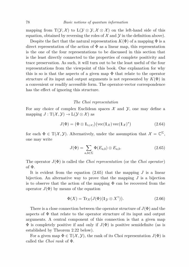
The Choi representationFor any choice of complex Euclidean spaces X and Y, one may define amapping J : T(X ,Y)→ L(Y ⊗ X ) as

J(Φ) =(Φ⊗ 1L(X )

)(vec(1X ) vec(1X )∗

)(2.64)

for each Φ ∈ T(X ,Y). Alternatively, under the assumption that X = CΣ,one may write

J(Φ) =∑

a,b∈ΣΦ(Ea,b)⊗ Ea,b. (2.65)

The operator J(Φ) is called the Choi representation (or the Choi operator)of Φ.

It is evident from the equation (2.65) that the mapping J is a linearbijection. An alternative way to prove that the mapping J is a bijectionis to observe that the action of the mapping Φ can be recovered from theoperator J(Φ) by means of the equation

Φ(X) = TrX(J(Φ)

(1Y ⊗XT)). (2.66)

There is a close connection between the operator structure of J(Φ) and theaspects of Φ that relate to the operator structure of its input and outputarguments. A central component of this connection is that a given mapΦ is completely positive if and only if J(Φ) is positive semidefinite (as isestablished by Theorem 2.22 below).

For a given map Φ ∈ T(X ,Y), the rank of its Choi representation J(Φ) iscalled the Choi rank of Φ.


Kraus representationsFor any choice of complex Euclidean spaces X and Y, an alphabet Σ, andcollections

Aa : a ∈ Σ and Ba : a ∈ Σ (2.67)

of operators drawn from the space L(X ,Y), one may define a linear mapΦ ∈ T(X ,Y) as

Φ(X) =∑

a∈ΣAaXB

∗a (2.68)

for every X ∈ L(X ). The expression (2.68) is a Kraus representation of themap Φ. It will be established shortly that a Kraus representation exists forevery map of the form Φ ∈ T(X ,Y). Unlike the natural representation andChoi representation, however, Kraus representations are not unique.

Under the assumption that Φ is determined by the above equation (2.68),it holds that

Φ∗(Y ) =∑

a∈ΣA∗aY Ba, (2.69)

as follows from a calculation relying on the cyclic property of the trace:⟨Y,∑

a∈ΣAaXB

∗a

⟩=∑

a∈ΣTr(Y ∗AaXB∗a

)

=∑

a∈ΣTr(B∗aY

∗AaX)

=⟨∑

a∈ΣA∗aY Ba, X

⟩ (2.70)

for every X ∈ L(X ) and Y ∈ L(Y).It is common in the theory of quantum information that one encounters

Kraus representations for which Aa = Ba for each a ∈ Σ. As is establishedby Theorem 2.22 below, such representations exist precisely when the mapbeing considered is completely positive.

Stinespring representationsSuppose X , Y, and Z are complex Euclidean spaces and A,B ∈ L(X ,Y⊗Z)are operators. One may then define a map Φ ∈ T(X ,Y) as

Φ(X) = TrZ(AXB∗

)(2.71)

for every X ∈ L(X ). The expression (2.71) is a Stinespring representationof the map Φ. Similar to Kraus representations, Stinespring representationsalways exist for a given map Φ, and are not unique.


If a map Φ ∈ T(X ,Y) has a Stinespring representation taking the form(2.71), then it holds that

Φ∗(Y ) = A∗(Y ⊗ 1Z)B (2.72)

for all Y ∈ L(Y). This observation follows from a calculation:

〈Y,Φ(X)〉 = 〈Y,TrZ(AXB∗)〉 = 〈Y ⊗ 1Z , AXB∗〉= Tr

((Y ⊗ 1Z)∗AXB∗

)= Tr

(B∗(Y ⊗ 1Z)∗AX

)

= 〈A∗(Y ⊗ 1Z)B,X〉(2.73)

for every X ∈ L(X ) and Y ∈ L(Y). Expressions of the form (2.72) arealso sometimes referred to as Stinespring representations (in this case of themap Φ∗), although the terminology will not be used in this way in this book.

Similar to Kraus representations, it is common in quantum informationtheory that one encounters Stinespring representations for which A = B.Also similar to Kraus representations, such representations exist if and onlyif Φ is completely positive.

Relationships among the representationsThe following proposition relates the four representations discussed aboveto one another, and (implicitly) shows how any one of the representationsmay be converted into any other.

Proposition 2.20 Let X and Y be complex Euclidean spaces, let Σ bean alphabet, let Aa : a ∈ Σ, Ba : a ∈ Σ ⊂ L(X ,Y) be collections ofoperators indexed by Σ, and let Φ ∈ T(X ,Y). The following four statements,which correspond as indicated to the four representations introduced above,are equivalent:

1. (Natural representation.) It holds that

K(Φ) =∑

a∈ΣAa ⊗Ba. (2.74)

2. (Choi representation.) It holds that

J(Φ) =∑

a∈Σvec(Aa) vec(Ba)∗. (2.75)

3. (Kraus representations.) It holds that

Φ(X) =∑

a∈ΣAaXB

∗a (2.76)

for all X ∈ L(X ).


4. (Stinespring representations.) For Z = CΣ and A,B ∈ L(X ,Y ⊗ Z)defined as

A =∑

a∈ΣAa ⊗ ea and B =

∑

a∈ΣBa ⊗ ea, (2.77)

it holds thatΦ(X) = TrZ

(AXB∗

)(2.78)

for all X ∈ L(X ).

Proof The equivalence between statements 3 and 4 is a straightforwardcalculation. The equivalence between statements 1 and 3 follows from theidentity

vec(AaXB∗a) =(Aa ⊗Ba

)vec(X) (2.79)

for all choices of a ∈ Σ and X ∈ L(X ). Finally, the equivalence betweenstatements 2 and 3 follows from the equations

(Aa ⊗ 1X ) vec(1X ) = vec(Aa),vec(1X )∗(B∗a ⊗ 1X ) = vec(Ba)∗,

(2.80)

which hold for every a ∈ Σ.

Corollary 2.21 Let X and Y be complex Euclidean spaces, let Φ ∈ T(X ,Y)be a nonzero linear map, and let r = rank(J(Φ)) be the Choi rank of Φ. Thefollowing two facts hold:

1. For Σ being any alphabet with |Σ| = r, there exists a Kraus representationof Φ having the form

Φ(X) =∑

a∈ΣAaXB

∗a, (2.81)

for some choice of Aa : a ∈ Σ, Ba : a ∈ Σ ⊂ L(X ,Y).2. For Z being any complex Euclidean space with dim(Z) = r, there exists

a Stinespring representation of Φ having the form

Φ(X) = TrZ(AXB∗

), (2.82)

for some choice of operators A,B ∈ L(X ,Y ⊗ Z).

Proof For Σ being any alphabet with |Σ| = r, it is possible to write

J(Φ) =∑

a∈Σuav∗a (2.83)


for some choice of vectors

ua : a ∈ Σ, va : a ∈ Σ ⊂ Y ⊗ X . (2.84)

In particular, one may take ua : a ∈ Σ to be any basis for the image ofJ(Φ), which uniquely determines a collection va : a ∈ Σ for which (2.83)holds. Taking Aa : a ∈ Σ and Ba : a ∈ Σ to be operators defined by theequations

vec(Aa) = ua and vec(Ba) = va (2.85)

for every a ∈ Σ, it follows from Proposition 2.20 that the expression (2.81)is a Kraus representation of Φ. Moreover, it holds that the expression (2.82)is a Stinespring representation of Φ for A,B ∈ L(X ,Y ⊗ Z) defined as

A =∑


∑

a∈ΣBa ⊗ ea, (2.86)

which completes the proof.

Characterizations of completely positive mapsCharacterizations of completely positive maps, based on their Choi, Kraus,and Stinespring representations, will now be presented.

Theorem 2.22 Let Φ ∈ T(X ,Y) be a nonzero map, for complex Euclideanspaces X and Y. The following statements are equivalent:

1. Φ is completely positive.2. Φ⊗ 1L(X ) is positive.3. J(Φ) ∈ Pos(Y ⊗ X ).4. There exists a collection Aa : a ∈ Σ ⊂ L(X ,Y), for some choice of

an alphabet Σ, for which

Φ(X) =∑

a∈ΣAaXA

∗a (2.87)

for all X ∈ L(X ).5. Statement 4 holds for an alphabet Σ satisfying |Σ| = rank(J(Φ)).6. There exists an operator A ∈ L(X ,Y ⊗Z), for some choice of a complex

Euclidean space Z, such that

Φ(X) = TrZ(AXA∗

)(2.88)

for all X ∈ L(X ).7. Statement 6 holds for Z having dimension equal to rank(J(Φ)).


Proof The theorem will be proved by establishing the following implicationsamong the seven statements, which are sufficient to imply their equivalence:

(1)⇒ (2)⇒ (3)⇒ (5)⇒ (4)⇒ (1)(5)⇒ (7)⇒ (6)⇒ (1)

Note that some of these implications are immediate: statement 1 impliesstatement 2 by the definition of complete positivity, statement 5 triviallyimplies statement 4, statement 7 trivially implies statement 6, and statement5 implies statement 7 by Proposition 2.20.

Assume Φ⊗ 1L(X ) is positive. Because

vec(1X ) vec(1X )∗ ∈ Pos(X ⊗ X ) (2.89)

andJ(Φ) = (Φ⊗ 1L(X ))(vec(1X ) vec(1X )∗), (2.90)

it follows that J(Φ) ∈ Pos(Y ⊗ X ), so statement 2 implies statement 3.Next, assume J(Φ) ∈ Pos(Y ⊗ X ). It follows by the spectral theorem

(Corollary 1.4), together with the fact that every eigenvalue of a positivesemidefinite operator is nonnegative, that one may write

J(Φ) =∑

a∈Σuau

∗a, (2.91)

for some choice of an alphabet Σ with |Σ| = rank(J(Φ)) and a collection

ua : a ∈ Σ ⊂ Y ⊗ X (2.92)

of vectors. Taking Aa ∈ L(X ,Y) to be the operator defined by the equationvec(Aa) = ua for each a ∈ Σ, one has that

J(Φ) =∑

a∈Σvec(Aa) vec(Aa)∗. (2.93)

The equation (2.87) therefore holds for every X ∈ L(X ) by Proposition 2.20,which establishes that statement 3 implies statement 5.

Now suppose (2.87) holds for every X ∈ L(X ), for some alphabet Σ anda collection

Aa : a ∈ Σ ⊂ L(X ,Y) (2.94)

of operators. For a complex Euclidean space W and a positive semidefiniteoperator P ∈ Pos(X ⊗W), it is evident that

(Aa ⊗ 1W)P (Aa ⊗ 1W)∗ ∈ Pos(Y ⊗W) (2.95)


for each a ∈ Σ, and therefore(Φ⊗ 1L(W)

)(P ) ∈ Pos(Y ⊗W) (2.96)

by the fact that Pos(Y⊗W) is a convex cone. It follows that Φ is completelypositive, so statement 4 implies statement 1.

Finally, suppose (2.88) holds for every X ∈ L(X ), for some complexEuclidean space Z and an operator A ∈ L(X ,Y ⊗ Z). For any complexEuclidean spaceW and any positive semidefinite operator P ∈ Pos(X ⊗W),it is again evident that

(A⊗ 1W)P (A⊗ 1W)∗ ∈ Pos(Y ⊗ Z ⊗W), (2.97)

so that(Φ⊗ 1L(W)

)(P ) = TrZ

((A⊗ 1W)P (A⊗ 1W)∗

) ∈ Pos(Y ⊗W) (2.98)

by the complete positivity of the trace (Corollary 2.19). It therefore holdsthat the map Φ is completely positive, so statement 6 implies statement 1,which completes the proof.

One consequence of this theorem is the following corollary, which relatesKraus representations of a given completely positive map.

Corollary 2.23 Let Σ be an alphabet, let X and Y be complex Euclideanspaces, and assume Aa : a ∈ Σ, Ba : a ∈ Σ ⊂ L(X ,Y) are collectionsof operators for which

∑

a∈ΣAaXA

∗a =

∑

a∈ΣBaXB

∗a (2.99)

for all X ∈ L(X ). There exists a unitary operator U ∈ U(CΣ) such that

Ba =∑

b∈ΣU(a, b)Ab (2.100)

for all a ∈ Σ.

Proof The maps

X 7→∑

a∈ΣAaXA

∗a and X 7→

∑

a∈ΣBaXB

∗a (2.101)

agree for all X ∈ L(X ), and therefore their Choi representations must beequal:

∑

a∈Σvec(Aa) vec(Aa)∗ =

∑

a∈Σvec(Ba) vec(Ba)∗. (2.102)


Let Z = CΣ and define vectors u, v ∈ Y ⊗ X ⊗ Z as

u =∑

a∈Σvec(Aa)⊗ ea and v =

∑

a∈Σvec(Ba)⊗ ea, (2.103)

so thatTrZ(uu∗) =

∑

a∈Σvec(Aa) vec(Aa)∗

=∑

a∈Σvec(Ba) vec(Ba)∗ = TrZ(vv∗).

(2.104)

By the unitary equivalence of purifications (Theorem 2.12), there must exista unitary operator U ∈ U(Z) such that

v = (1Y⊗X ⊗ U)u. (2.105)

Thus, for each a ∈ Σ it holds that

vec(Ba) = (1Y⊗X ⊗ e∗a)v = (1Y⊗X ⊗ e∗aU)u =∑

b∈ΣU(a, b) vec(Ab), (2.106)

which is equivalent to (2.100).

Along similar lines to the previous corollary is the following one, whichconcerns Stinespring representations rather than Kraus representations. Asthe proof reveals, the two corollaries are essentially equivalent.

Corollary 2.24 Let X , Y, and Z be complex Euclidean spaces and letoperators A,B ∈ L(X ,Y ⊗ Z) satisfy the equation

TrZ(AXA∗

)= TrZ

(BXB∗

)(2.107)

for every X ∈ L(X ). There exists a unitary operator U ∈ U(Z) such that

B = (1Y ⊗ U)A. (2.108)

Proof Let Σ be the alphabet for which Z = CΣ, and define two collectionsAa : a ∈ Σ, Ba : a ∈ Σ ⊂ L(X ,Y) of operators as

Aa = (1Y ⊗ e∗a)A and Ba = (1Y ⊗ e∗a)B, (2.109)

for each a ∈ Σ, so that

A =∑


∑

a∈ΣBa ⊗ ea. (2.110)

The equation (2.107) is equivalent to (2.99) in Corollary 2.23. It followsfrom that corollary that there exists a unitary operator U ∈ U(Z) such that(2.100) holds, which is equivalent to B = (1Y ⊗ U)A.


A map Φ ∈ T(X ,Y) is said to be Hermitian preserving if it holds thatΦ(H) ∈ Herm(Y) for all H ∈ Herm(X ). The following theorem, whichprovides four alternative characterizations of this class of maps, is provedthrough the use of Theorem 2.22.

Theorem 2.25 Let Φ ∈ T(X ,Y) be a map, for complex Euclidean spacesX and Y. The following statements are equivalent:

1. Φ is Hermitian preserving.2. It holds that (Φ(X))∗ = Φ(X∗) for every X ∈ L(X ).3. It holds that J(Φ) ∈ Herm(Y ⊗ X ).4. There exist completely positive maps Φ0,Φ1 ∈ CP(X ,Y) for which

Φ = Φ0 − Φ1.5. There exist positive maps Φ0,Φ1 ∈ T(X ,Y) for which Φ = Φ0 − Φ1.

Proof Assume first that Φ is a Hermitian-preserving map. For an arbitraryoperator X ∈ L(X ), one may write X = H + iK for H,K ∈ Herm(X ) beingdefined as

H = X +X∗

2 and K = X −X∗2i . (2.111)

As Φ(H) and Φ(K) are both Hermitian and Φ is linear, it follows that

(Φ(X))∗ = (Φ(H) + iΦ(K))∗

= Φ(H)− iΦ(K) = Φ(H − iK) = Φ(X∗).(2.112)

Statement 1 therefore implies statement 2.Next, assume statement 2 holds, and let Σ be the alphabet for whichX = CΣ. One then has that

J(Φ)∗ =∑

a,b∈ΣΦ(Ea,b)∗ ⊗ E∗a,b =

∑

a,b∈ΣΦ(E∗a,b)⊗ E∗a,b

=∑

a,b∈ΣΦ(Eb,a)⊗ Eb,a = J(Φ).

(2.113)

It follows that J(Φ) is Hermitian, and therefore statement 3 holds.Now assume statement 3 holds. Let J(Φ) = P0 − P1 be the Jordan–Hahn

decomposition of J(Φ), and let Φ0,Φ1 ∈ CP(X ,Y) be the maps for whichJ(Φ0) = P0 and J(Φ1) = P1. Because P0 and P1 are positive semidefinite,it follows from Theorem 2.22 that Φ0 and Φ1 are completely positive maps.By the linearity of the mapping J associated with the Choi representation,it holds that J(Φ) = J(Φ0−Φ1), and therefore Φ = Φ0−Φ1, implying thatstatement 4 holds.

Statement 4 trivially implies statement 5.


Finally, assume statement 5 holds. Let H ∈ Herm(X ) be a Hermitianoperator, and let H = P0 − P1, for P0, P1 ∈ Pos(X ), be the Jordan–Hahndecomposition of H. It holds that Φa(Pb) ∈ Pos(Y), for all a, b ∈ 0, 1, bythe positivity of Φ0 and Φ1. Therefore, one has that

Φ(H) =(Φ0(P0) + Φ1(P1)

)− (Φ0(P1) + Φ1(P0))

(2.114)

is the difference between two positive semidefinite operators, and is thereforeHermitian. Thus, statement 1 holds.

As the implications (1) ⇒ (2) ⇒ (3) ⇒ (4) ⇒ (5) ⇒ (1) among thestatements have been established, the theorem is proved.

Characterizations of trace-preserving mapsThe next theorem provides multiple characterizations of the class of trace-preserving maps.

Theorem 2.26 Let Φ ∈ T(X ,Y) be a map, for complex Euclidean spacesX and Y. The following statements are equivalent:

1. Φ is a trace-preserving map.2. Φ∗ is a unital map.3. TrY

(J(Φ)

)= 1X .

4. There exist collections Aa : a ∈ Σ, Ba : a ∈ Σ ⊂ L(X ,Y) ofoperators such that

Φ(X) =∑

a∈ΣAaXB

∗a (2.115)

and∑

a∈ΣA∗aBa = 1X . (2.116)

5. For all collections Aa : a ∈ Σ, Ba : a ∈ Σ ⊂ L(X ,Y) of operatorssatisfying (2.115), the equation (2.116) must also hold.

6. There exist operators A,B ∈ L(X ,Y ⊗ Z), for some complex Euclideanspace Z, such that

Φ(X) = TrZ(AXB∗

)(2.117)

and A∗B = 1X .7. For every choice of operators A,B ∈ L(X ,Y ⊗ Z) satisfying (2.117), it

holds that A∗B = 1X .


Proof Under the assumption that Φ preserves trace, it holds that

〈1X , X〉 = Tr(X) = Tr(Φ(X)) = 〈1Y ,Φ(X)〉 = 〈Φ∗(1Y), X〉, (2.118)

and therefore〈1X − Φ∗(1Y), X〉 = 0, (2.119)

for all X ∈ L(X ). It follows that Φ∗(1Y) = 1X , and therefore Φ∗ is unital.Along similar lines, the assumption that Φ∗ is unital implies

Tr(Φ(X)) = 〈1Y ,Φ(X)〉 = 〈Φ∗(1Y), X〉 = 〈1X , X〉 = Tr(X) (2.120)

for every X ∈ L(X ), and therefore Φ preserves trace. The equivalence ofstatements 1 and 2 has been established.

Next, assume that Aa : a ∈ Σ, Ba : a ∈ Σ ⊂ L(X ,Y) satisfy

Φ(X) =∑

a∈ΣAaXB

∗a (2.121)

for all X ∈ L(X ). It therefore holds that

Φ∗(Y ) =∑

a∈ΣA∗aY Ba (2.122)

for every Y ∈ L(Y), and in particular it holds that

Φ∗(1Y) =∑

a∈ΣA∗aBa. (2.123)

Thus, if Φ∗ is a unital map, then∑

a∈ΣA∗aBa = 1X , (2.124)

and so it has been proved that statement 2 implies statement 5. On theother hand, if (2.124) holds, then it follows that Φ∗(1Y) = 1X , so that Φ∗ isunital. Therefore, statement 4 implies statement 2. As statement 5 impliesstatement 4, by virtue of the fact that Kraus representations exist for everymap, the equivalence of statements 2, 4, and 5 has been established.

Now assume that A,B ∈ L(X ,Y ⊗ Z) satisfy Φ(X) = TrZ(AXB∗

)for

every X ∈ L(X ). It follows that

Φ∗(Y ) = A∗(Y ⊗ 1Z)B (2.125)

for all Y ∈ L(Y), and in particular Φ∗(1Y) = A∗B. The equivalence ofstatements 2, 6, and 7 follows by the same reasoning as for the case ofstatements 2, 4, and 5.


Finally, let Γ be the alphabet for which X = CΓ, and consider the operator

TrY(J(Φ)) =∑

a,b∈ΓTr(Φ(Ea,b))Ea,b. (2.126)

If Φ preserves trace, then it follows that

Tr(Φ(Ea,b)) =

1 if a = b

0 if a 6= b,(2.127)

and therefore

TrY(J(Φ)) =∑

a∈ΓEa,a = 1X . (2.128)

Conversely, if TrY(J(Φ)) = 1X , then a consideration of the expression(2.126) reveals that (2.127) must hold. As the set Ea,b : a, b ∈ Γ is abasis of L(X ), one concludes by linearity that Φ preserves trace. Statements1 and 3 are therefore equivalent, which completes the proof.

Characterizations of channelsTheorems 2.22 and 2.26 can be combined, providing characterizations ofchannels based on their Choi, Kraus, and Stinespring representations.

Corollary 2.27 Let Φ ∈ T(X ,Y) be a map, for complex Euclidean spacesX and Y. The following statements are equivalent:

1. Φ is a channel.2. J(Φ) ∈ Pos(Y ⊗ X ) and TrY(J(Φ)) = 1X .3. There exists an alphabet Σ and a collection Aa : a ∈ Σ ⊂ L(X ,Y)

satisfying∑

a∈ΣA∗aAa = 1X and Φ(X) =

∑

a∈ΣAaXA

∗a (2.129)

for all X ∈ L(X ).4. Statement 3 holds for |Σ| = rank(J(Φ)).5. There exists an isometry A ∈ U(X ,Y⊗Z), for some choice of a complex

Euclidean space Z, such that

Φ(X) = TrZ(AXA∗

)(2.130)

for all X ∈ L(X ).6. Statement 5 holds under the requirement dim(Z) = rank(J(Φ)).


For every choice of complex Euclidean spaces X and Y, one has that theset of channels C(X ,Y) is compact and convex. One way to prove this factmakes use of the previous corollary.

Proposition 2.28 Let X and Y be complex Euclidean spaces. The setC(X ,Y) is compact and convex.

Proof The map J : T(X ,Y)→ L(Y ⊗ X ) defining the Choi representationis linear and invertible. By Corollary 2.27, one has J−1(A) = C(X ,Y) for Abeing defined as

A =X ∈ Pos(Y ⊗ X ) : TrY(X) = 1X

. (2.131)

It therefore suffices to prove that A is compact and convex. It is evident thatA is closed and convex, as it is the intersection of the positive semidefinitecone Pos(Y ⊗ X ) with the affine subspace

X ∈ L(Y ⊗ X ) : TrY(X) = 1X

, (2.132)

both of which are closed and convex. To complete the proof, it suffices toprove that A is bounded. For every X ∈ A, one has

‖X‖1 = Tr(X) = Tr(TrY(X)

)= Tr

(1X)

= dim(X ), (2.133)

and therefore A is bounded, as required.

Corollary 2.27 will be used frequently throughout this book, sometimesimplicitly. The next proposition, which builds on the unitary equivalenceof purifications (Theorem 2.12) to relate a given purification of a positivesemidefinite operator to any extension of that operator, is one example ofan application of this corollary.

Proposition 2.29 Let X , Y, and Z be complex Euclidean spaces, andsuppose that u ∈ X ⊗ Y and P ∈ Pos(X ⊗ Z) satisfy

TrY(uu∗

)= TrZ(P ). (2.134)

There exists a channel Φ ∈ C(Y,Z) such that(1L(X ) ⊗ Φ

)(uu∗) = P. (2.135)

Proof Let W be a complex Euclidean space having dimension sufficientlylarge so that

dim(W) ≥ rank(P ) and dim(Z ⊗W) ≥ dim(Y), (2.136)


and let A ∈ U(Y,Z ⊗W) be any isometry. Also let v ∈ X ⊗ Z ⊗W satisfyTrW

(vv∗

)= P . It holds that

TrZ⊗W((1X ⊗A

)uu∗

(1X ⊗A

)∗)

= TrY(uu∗

)= TrZ(P ) = TrZ⊗W

(vv∗

).

(2.137)

By Theorem 2.12 there must exist a unitary operator U ∈ U(Z ⊗W) suchthat

(1X ⊗ UA

)u = v. (2.138)

Define Φ ∈ T(Y,Z) as

Φ(Y ) = TrW((UA)Y (UA)∗

)(2.139)

for all Y ∈ L(Y). By Corollary 2.27, one has that Φ is a channel. It holdsthat

(1L(X ) ⊗ Φ

)(uu∗) = TrW

((1X ⊗ UA)uu∗(1X ⊗ UA)∗

)

= TrW(vv∗

)= P,

(2.140)

as required.

2.2.3 Examples of channels and other mappingsThis section describes examples of channels, and other maps, along withtheir specifications according to the four types of representations discussedabove. Many other examples and general classifications of channels and mapswill be encountered throughout the book.

Isometric and unitary channelsLet X and Y be complex Euclidean spaces, let A,B ∈ L(X ,Y) be operators,and consider the map Φ ∈ T(X ,Y) defined by

Φ(X) = AXB∗ (2.141)

for all X ∈ L(X ).In the case that A = B, and assuming in addition that this operator is

a linear isometry from X to Y, it follows from Corollary 2.27 that Φ is achannel. Such a channel is said to be an isometric channel. If Y = X andA = B is a unitary operator, Φ is said to be a unitary channel. Unitarychannels, and convex combinations of unitary channels, are discussed ingreater detail in Chapter 4.


The natural representation of the map Φ defined by (2.141) is

K(Φ) = A⊗B (2.142)

and the Choi representation of Φ is

J(Φ) = vec(A) vec(B)∗. (2.143)

The expression (2.141) is a Kraus representation of Φ, and may also beregarded as a trivial example of a Stinespring representation if one takesZ = C and observes that the trace acts as the identity mapping on C.

The identity mapping 1L(X ) is a simple example of a unitary channel. Thenatural representation of this channel is the identity operator 1X⊗1X , whileits Choi representation is given by the rank-one operator vec(1X ) vec(1X )∗.

Replacement channels and the completely depolarizing channelLet X and Y be complex Euclidean spaces, let A ∈ L(X ) and B ∈ L(Y) beoperators, and consider the map Φ ∈ T(X ,Y) defined as

Φ(X) = 〈A,X〉B (2.144)

for all X ∈ L(X ). The natural representation of Φ is

K(Φ) = vec(B) vec(A)∗, (2.145)

and the Choi representation of Φ is

J(Φ) = B ⊗A. (2.146)

Kraus and Stinespring representations of Φ may also be constructed,although they are not necessarily enlightening in this particular case. Oneway to obtain a Kraus representation of Φ is to first write

A =∑

a∈Σuax

∗a and B =

∑

b∈Γvby∗b , (2.147)

for some choice of alphabets Σ and Γ and four sets of vectors:

ua : a ∈ Σ, xa : a ∈ Σ ⊂ X ,vb : b ∈ Γ, yb : b ∈ Γ ⊂ Y.

(2.148)

It then follows that one Kraus representation of Φ is given by

Φ(X) =∑

(a,b)∈Σ×ΓCa,bXD

∗a,b (2.149)


where Ca,b = vbu∗a and Da,b = ybx

∗a for each a ∈ Σ and b ∈ Γ, and one

Stinespring representation is given by

Φ(X) = TrZ(CXD∗), (2.150)

where

C =∑

(a,b)∈Σ×ΓCa,b ⊗ e(a,b), D =

∑

(a,b)∈Σ×ΓDa,b ⊗ e(a,b), (2.151)

and Z = CΣ×Γ.If A and B are positive semidefinite operators and the map Φ ∈ T(X ,Y)

is defined by (2.144) for all X ∈ L(X ), then J(Φ) = B ⊗ A is positivesemidefinite, and therefore Φ is completely positive by Theorem 2.22. In thecase that A = 1X and B = σ for some density operator σ ∈ D(Y), the mapΦ is also trace preserving, and is therefore a channel. Such a channel is areplacement channel: it effectively discards its input, replacing it with thestate σ.

The completely depolarizing channel Ω ∈ C(X ) is an important exampleof a replacement channel. This channel is defined as

Ω(X) = Tr(X)ω (2.152)

for all X ∈ L(X ), where

ω = 1Xdim(X ) (2.153)

denotes the completely mixed state defined with respect to the space X .Equivalently, Ω is the unique channel transforming every density operatorinto this completely mixed state: Ω(ρ) = ω for all ρ ∈ D(X ). From theequations (2.145) and (2.146), one has that the natural representation ofthe completely depolarizing channel Ω ∈ C(X ) is

K(Ω) = vec(1X ) vec(1X )∗dim(X ) , (2.154)

while the Choi representation of this channel is

J(Ω) = 1X ⊗ 1Xdim(X ) . (2.155)

The transpose mapLet Σ be an alphabet, let X = CΣ, and let T ∈ T(X ) denote the transposemap, defined as

T(X) = XT (2.156)


for all X ∈ L(X ). This map will play an important role in Chapter 6, dueto its connections to properties of entangled states.

The natural representation K(T) of T must, by definition, satisfy

K(T) vec(X) = vec(XT) (2.157)

for all X ∈ L(X ). By considering those operators of the form X = uvT forvectors u, v ∈ X , one finds that

K(T)(u⊗ v) = v ⊗ u. (2.158)

It follows that K(T) = W , for W ∈ L(X ⊗ X ) being the swap operator,which is defined by the action W (u⊗ v) = v ⊗ u for all vectors u, v ∈ X .

The Choi representation of T is also equal to the swap operator, as

J(T) =∑

a,b∈ΣEb,a ⊗ Ea,b = W. (2.159)

Under the assumption that |Σ| ≥ 2, it therefore follows from Theorem 2.22that T is not a completely positive map, as W is not a positive semidefiniteoperator in this case.

One example of a Kraus representation of T is

T(X) =∑

a,b∈ΣEa,bXE

∗b,a (2.160)

for all X ∈ L(X ), from which it follows that T(X) = TrZ(AXB∗) is aStinespring representation of T for Z = CΣ×Σ,

A =∑

a,b∈ΣEa,b ⊗ e(a,b), and B =

∑

a,b∈ΣEb,a ⊗ e(a,b). (2.161)

The completely dephasing channelLet Σ be an alphabet and let X = CΣ. The map ∆ ∈ T(X ) defined as

∆(X) =∑

a∈ΣX(a, a)Ea,a (2.162)

for every X ∈ L(X ) is an example of a channel known as the completelydephasing channel. This channel has the effect of replacing every off-diagonalentry of a given operator X ∈ L(X ) by 0 and leaving the diagonal entriesunchanged.

Through the association of diagonal density operators with probabilisticstates, as discussed in Section 2.1.2, one may view the channel ∆ as anideal channel for classical communication: it acts as the identity mappingon every diagonal density operator, so that it effectively transmits classical


probabilistic states without error, while all other states are mapped to theprobabilistic state given by their diagonal entries.

The natural representation of ∆ must satisfy the equation

K(∆) vec(Ea,b) =

vec(Ea,b) if a = b

0 if a 6= b,(2.163)

which is equivalent to

K(∆)(ea ⊗ eb) =

ea ⊗ eb if a = b

0 if a 6= b,(2.164)

for every a, b ∈ Σ. It follows that

K(∆) =∑

a∈ΣEa,a ⊗ Ea,a. (2.165)

Similar to the transpose mapping, the Choi representation of ∆ happensto coincide with its natural representation, as the calculation

J(∆) =∑

a,b∈Σ∆(Ea,b)⊗ Ea,b =

∑

a∈ΣEa,a ⊗ Ea,a (2.166)

reveals. It is evident from this expression, together with Corollary 2.27, that∆ is indeed a channel.

One example of a Kraus representation of ∆ is

∆(X) =∑

a∈ΣEa,aXE

∗a,a, (2.167)

and an example of a Stinespring representation of ∆ is

∆(X) = TrZ(AXA∗

)(2.168)

for Z = CΣ andA =

∑

a∈Σ(ea ⊗ ea)e∗a. (2.169)

A digression on classical registersClassical probabilistic states of registers may be associated with diagonaldensity operators, as discussed in Section 2.1.2. The term classical registerwas mentioned in that discussion but not fully explained. It is appropriateto make this notion more precise, now that channels (and the completelydephasing channel in particular) have been introduced.

From a mathematical point of view, classical registers are not defined in amanner that is distinct from ordinary (quantum) registers. Rather, the term


classical register will be used to refer to any register that, by the nature ofthe processes under consideration, would be unaffected by an application ofthe completely dephasing channel ∆ at any moment during its existence.Every state of a classical register is necessarily a diagonal density operator,corresponding to a probabilistic state, as these are the density operators thatare invariant under the action of the channel ∆. Moreover, the correlationsthat may exist between a classical register and one or more other registersare limited. For example, for a classical register X and an arbitrary registerY, the only states of the compound register (X,Y) that are consistent withthe term classical register being applied to X are those taking the form

∑

a∈Σp(a)Ea,a ⊗ ρa, (2.170)

for Σ being the classical state set of X, ρa : a ∈ Σ ⊆ D(Y) being anarbitrary collection of states of Y, and p ∈ P(Σ) being a probability vector.States of this form are commonly called classical-quantum states. It is bothnatural and convenient in some situations to associate the state (2.170) withthe ensemble η : Σ→ Pos(Y) defined as η(a) = p(a)ρa for each a ∈ Σ.

2.2.4 Extremal channelsFor any choice of complex Euclidean spaces X and Y, the set of channelsC(X ,Y) is compact and convex (by Proposition 2.28). A characterization ofthe extreme points of this set is given by Theorem 2.31 below. The followinglemma will be used in the proof of this theorem.

Lemma 2.30 Let A ∈ L(Y,X ) be an operator, for complex Euclideanspaces X and Y. It holds that

P ∈ Pos(X ) : im(P ) ⊆ im(A)

=AQA∗ : Q ∈ Pos(Y)

. (2.171)

Proof For every Q ∈ Pos(Y), it holds that AQA∗ is positive semidefiniteand satisfies im(AQA∗) ⊆ im(A). The set on the right-hand side of (2.171)is therefore contained in the set on the left-hand side.

For the reverse containment, if P ∈ Pos(X ) satisfies im(P ) ⊆ im(A), thenby setting

Q = A+P (A+)∗, (2.172)

for A+ denoting the Moore–Penrose pseudo-inverse of A, one obtains

AQA∗ = (AA+)P (AA+)∗ = Πim(A)PΠim(A) = P, (2.173)

which completes the proof.


Theorem 2.31 (Choi) Let X and Y be complex Euclidean spaces, letΦ ∈ C(X ,Y) be a channel, and let Aa : a ∈ Σ ⊂ L(X ,Y) be a linearlyindependent set of operators satisfying

Φ(X) =∑

a∈ΣAaXA

∗a (2.174)

for all X ∈ L(X ). The channel Φ is an extreme point of the set C(X ,Y) ifand only if the collection

A∗bAa : (a, b) ∈ Σ× Σ

⊂ L(X ) (2.175)

of operators is linearly independent.

Proof Let Z = CΣ, define an operator M ∈ L(Z,Y ⊗ X ) as

M =∑

a∈Σvec(Aa)e∗a, (2.176)

and observe that

MM∗ =∑

a∈Σvec(Aa) vec(Aa)∗ = J(Φ). (2.177)

As Aa : a ∈ Σ is a linearly independent collection of operators, it musthold that ker(M) = 0.

Assume first that Φ is not an extreme point of C(X ,Y). It follows thatthere exist channels Ψ0,Ψ1 ∈ C(X ,Y), with Ψ0 6= Ψ1, along with a scalarλ ∈ (0, 1), such that

Φ = λΨ0 + (1− λ)Ψ1. (2.178)

Let P = J(Φ), Q0 = J(Ψ0), and Q1 = J(Ψ1), so that

P = λQ0 + (1− λ)Q1. (2.179)

As Φ, Ψ0, and Ψ1 are channels, the operators P,Q0, Q1 ∈ Pos(Y ⊗ X ) arepositive semidefinite and satisfy

TrY(P ) = TrY(Q0) = TrY(Q1) = 1X , (2.180)

by Corollary 2.27.As λ is positive and the operators Q0 and Q1 are positive semidefinite,

the equation (2.179) implies

im(Q0) ⊆ im(P ) = im(M). (2.181)

It follows by Lemma 2.30 that there exists a positive semidefinite operatorR0 ∈ Pos(Z) for which Q0 = MR0M∗. By similar reasoning, there exists apositive semidefinite operator R1 ∈ Pos(Z) for which Q1 = MR1M∗.


Letting H = R0 −R1, one finds that

0 = TrY(Q0)− TrY(Q1) = TrY(MHM∗

)=∑

a,b∈ΣH(a, b)

(A∗bAa

)T, (2.182)

and therefore∑

a,b∈ΣH(a, b)A∗bAa = 0. (2.183)

Because Ψ0 6= Ψ1, it holds that Q0 6= Q1, so R0 6= R1, and therefore H 6= 0.It has therefore been proved that

A∗bAa : (a, b) ∈ Σ × Σ

is a linearly

dependent collection of operators.Now assume the set (2.175) is linearly dependent:

∑

a,b∈ΣZ(a, b)A∗bAa = 0 (2.184)

for some choice of a nonzero operator Z ∈ L(Z). By taking the adjoint ofboth sides of this equation, one finds that

∑

a,b∈ΣZ∗(a, b)A∗bAa = 0, (2.185)

from which it follows that∑

a,b∈ΣH(a, b)A∗bAa = 0 (2.186)

for both of the Hermitian operators

H = Z + Z∗

2 and H = Z − Z∗2i . (2.187)

At least one of these operators must be nonzero, which implies that (2.186)must hold for some choice of a nonzero Hermitian operator H. Let such achoice of H be fixed, and assume moreover that ‖H‖ = 1 (which causes noloss of generality as (2.186) still holds if H is replaced by H/‖H‖).

Let Ψ0,Ψ1 ∈ T(X ,Y) be the mappings defined by the equations

J(Ψ0) = M(1 +H)M∗ and J(Ψ1) = M(1−H)M∗. (2.188)

Because H is Hermitian and satisfies ‖H‖ = 1, one has that the operators1+H and 1−H are both positive semidefinite. The operators M(1+H)M∗and M(1−H)M∗ are therefore positive semidefinite as well, implying that


Ψ0 and Ψ1 are completely positive, by Theorem 2.22. It holds that

TrY (MHM∗) =∑

a,b∈ΣH(a, b) (A∗bAa)

T

=( ∑

a,b∈ΣH(a, b)A∗bAa

)T

= 0(2.189)

and therefore the following two equations hold:

TrY (J(Ψ0)) = TrY (MM∗) + TrY (MHM∗) = TrY(J(Φ)) = 1X ,

TrY (J(Ψ1)) = TrY (MM∗)− TrY (MHM∗) = TrY(J(Φ)) = 1X .(2.190)

Thus, Ψ0 and Ψ1 are trace preserving by Theorem 2.26, and are thereforechannels.

Finally, given that H 6= 0 and ker(M) = 0, it holds that J(Ψ0) 6= J(Ψ1),so that Ψ0 6= Ψ1. As

12J(Ψ0) + 1

2J(Ψ1) = MM∗ = J(Φ), (2.191)

one has that

Φ = 12Ψ0 + 1

2Ψ1, (2.192)

which demonstrates that Φ is not an extreme point of C(X ,Y).

Example 2.32 Let X and Y be complex Euclidean spaces such thatdim(X ) ≤ dim(Y), let A ∈ U(X ,Y) be an isometry, and let Φ ∈ C(X ,Y) bethe isometric channel defined by

Φ(X) = AXA∗ (2.193)

for all X ∈ L(X ). The set A∗A contains a single nonzero operator, and istherefore linearly independent. By Theorem 2.31, Φ is an extreme point ofthe set C(X ,Y).

Example 2.33 Let Σ = 0, 1 denote the binary alphabet, and let X = CΣ

and Y = CΣ×Σ. Also define operators A0, A1 ∈ L(X ,Y) as

A0 = 1√6(2E00,0 + E01,1 + E10,1

),

A1 = 1√6(2E11,1 + E01,0 + E10,0

).

(2.194)

(Elements of the form (a, b) ∈ Σ×Σ have been written as ab for the sake of


clarity.) Expressed as matrices (with respect to the natural orderings of Σand Σ× Σ), these operators are as follows:

A0 = 1√6

2 00 10 10 0

and A1 = 1√

6

0 01 01 00 2

. (2.195)

Now, define a channel Φ ∈ C(X ,Y) as

Φ(X) = A0XA∗0 +A1XA

∗1 (2.196)

for every X ∈ L(X ). It holds that

A∗0A0 = 13

(2 00 1

), A∗0A1 = 1

3

(0 01 0

),

A∗1A0 = 13

(0 10 0

), A∗1A1 = 1

3

(1 00 2

).

(2.197)

The setA∗0A0, A

∗0A1, A

∗1A0, A

∗1A1

(2.198)

is linearly independent, and therefore Theorem 2.31 implies that Φ is anextreme point of C(X ,Y).

2.3 MeasurementsMeasurements provide the mechanism through which classical informationmay be extracted from quantum states. This section defines measurements,and various notions connected with measurements, and provides a basicmathematical development of this concept.

2.3.1 Two equivalent definitions of measurementsWhen a hypothetical observer measures a register, the observer obtains aclassical measurement outcome (as opposed to a description of the state ofthe register, for instance). In general, this measurement outcome is generatedat random, according to a probability distribution that is determined bythe measurement together with the state of the register immediately beforethe measurement was performed. In this way, measurements allow one toassociate a meaning to the density operator description of quantum states,

2.3 Measurements 101

at least insofar as the density operators determine the probabilities withwhich different classical outcomes occur for each possible measurement.

Measurements can be defined in mathematical terms in two different,but equivalent, ways. Both ways will be described in this section, and theirequivalence will be explained.

Measurements defined by measurement operatorsThe following definition represents the first formulation of measurements tobe described in this book. The precise mathematical meaning of the termmeasurement used throughout this book coincides with this definition.

Definition 2.34 A measurement is a function of the form

µ : Σ→ Pos(X ), (2.199)

for some choice of an alphabet Σ and a complex Euclidean space X , satisfyingthe constraint

∑

a∈Σµ(a) = 1X . (2.200)

The set Σ is the set of measurement outcomes of this measurement, andeach operator µ(a) is the measurement operator associated with the outcomea ∈ Σ.

When a measurement µ is performed on a given register X, it must beassumed that µ takes the form (2.199), for some choice of an alphabet Σand for X being the complex Euclidean space associated with X. Two thingshappen when such a measurement is performed, assuming the state of Ximmediately prior to the measurement is ρ ∈ D(X ):

1. An element of Σ is selected at random. The probability distribution thatdescribes this random selection is represented by the probability vectorp ∈ P(Σ) defined as

p(a) = 〈µ(a), ρ〉 (2.201)

for each a ∈ Σ.2. The register X ceases to exist, in the sense that it no longer has a defined

state and cannot be considered in further calculations.

It is evident from the first item that the probabilities associated withthe outcomes of a given measurement depend linearly on the state that ismeasured. It is also evident that the probability vector p ∈ P(Σ) definedby (2.201) is indeed a probability vector: as ρ and µ(a) are both positive


semidefinite, their inner product 〈µ(a), ρ〉 is nonnegative, and summing thesevalues gives

∑

a∈Σp(a) =

∑

a∈Σ〈µ(a), ρ〉 = 〈1X , ρ〉 = Tr(ρ) = 1. (2.202)

The assumption that registers cease to exist after being measured is notuniversal within quantum information theory—an alternative definition, inwhich the states of registers after they are measured is specified, does notmake this requirement. Measurements of this alternative type, which arecalled nondestructive measurements in this book, are discussed in greaterdetail in Section 2.3.2. Nondestructive measurements can, however, bedescribed as compositions of ordinary measurements (as described above)and channels. For this reason, no generality is lost in making the assumptionthat registers cease to exist upon being measured.

It is sometimes convenient to specify a measurement by describing itsmeasurement operators as a collection indexed by its set of measurementoutcomes. In particular, when one refers to a measurement as a collection

Pa : a ∈ Σ ⊂ Pos(X ), (2.203)

it is to be understood that the measurement is given by µ : Σ → Pos(X ),where µ(a) = Pa for each a ∈ Σ.

Measurements as channelsThe second formulation of measurements, which is equivalent to the first,essentially describes measurements as channels whose outputs are stored inclassical registers. The following definition of quantum-to-classical channelsmakes this notion precise.

Definition 2.35 Let Φ ∈ C(X ,Y) be a channel, for complex Euclideanspaces X and Y. It is said that Φ is a quantum-to-classical channel if

Φ = ∆Φ, (2.204)

for ∆ ∈ C(Y) denoting the completely dephasing channel, defined withrespect to the space Y.

An equivalent condition for a channel Φ ∈ C(X ,Y) to be a quantum-to-classical channel is that Φ(ρ) is a diagonal density operator for everyρ ∈ D(X ). The following simple proposition establishes that this is so.

Proposition 2.36 Let Φ ∈ C(X ,Y) be a channel, for complex Euclideanspaces X and Y. It holds that Φ is a quantum-to-classical channel if andonly if Φ(ρ) is diagonal for every ρ ∈ D(X ).


Proof If Φ is a quantum-to-classical channel, then

Φ(ρ) = ∆(Φ(ρ)), (2.205)

and therefore Φ(ρ) is diagonal, for every density operator ρ ∈ D(X ).Conversely, if Φ(ρ) is diagonal, then Φ(ρ) = ∆(Φ(ρ)), and therefore

(Φ−∆Φ)(ρ) = 0, (2.206)

for every ρ ∈ D(X ). As the density operators D(X ) span all of L(X ), itfollows that Φ = ∆Φ, and therefore Φ is a quantum-to-classical channel.

The next theorem reveals the equivalence between quantum-to-classicalchannels and measurements. In essence, quantum-to-classical channels of theform Φ ∈ C(X ,Y) represent precisely those channels that can be realized asa measurement of a register X, according to a measurement µ : Σ→ Pos(X ),followed by the measurement outcome being stored in a register Y havingclassical state set Σ.

Theorem 2.37 Let X be a complex Euclidean space, let Σ be an alphabet,and let Y = CΣ. The following two complementary facts hold:

1. For every quantum-to-classical channel Φ ∈ C(X ,Y), there exists aunique measurement µ : Σ→ Pos(X ) for which the equation

Φ(X) =∑

a∈Σ〈µ(a), X〉Ea,a (2.207)

holds for all X ∈ L(X ).2. For every measurement µ : Σ → Pos(X ), the mapping Φ ∈ T(X ,Y)

defined by (2.207) for all X ∈ L(X ) is a quantum-to-classical channel.

Proof Assume first that Φ ∈ C(X ,Y) is a quantum-to-classical channel. Ittherefore holds that

Φ(X) = ∆(Φ(X)) =∑

a∈Σ〈Ea,a,Φ(X)〉Ea,a =

∑

a∈Σ〈Φ∗(Ea,a), X〉Ea,a (2.208)

for all X ∈ L(X ). Define a function µ : Σ→ L(X ) as

µ(a) = Φ∗(Ea,a) (2.209)

for each a ∈ Σ. As Φ is positive, so too is Φ∗ (by Proposition 2.18), andtherefore µ(a) ∈ Pos(X ) for each a ∈ Σ. Moreover, as Φ preserves trace, itholds (by Theorem 2.26) that Φ∗ is unital, and therefore

∑

a∈Σµ(a) =

∑

a∈ΣΦ∗(Ea,a) = Φ∗(1Y) = 1X . (2.210)


It follows that µ is a measurement for which (2.207) holds for all X ∈ L(X ).Toward proving the uniqueness of the measurement µ satisfying (2.207)

for all X ∈ L(X ), let ν : Σ → Pos(X ) be an arbitrary measurement forwhich the equation

Φ(X) =∑

a∈Σ〈ν(a), X〉Ea,a (2.211)

holds for all X ∈ L(X ). One then has that∑

a∈Σ〈µ(a)− ν(a), X〉Ea,a = 0 (2.212)

for all X ∈ L(X ), which implies that ν(a) = µ(a) for every a ∈ Σ, andcompletes the proof of the first fact.

Now assume that µ : Σ→ Pos(X ) is a measurement, and let Φ ∈ T(X ,Y)be defined by (2.207). The Choi representation of this map is

J(Φ) =∑

a∈ΣEa,a ⊗ µ(a). (2.213)

This is a positive semidefinite operator, and it holds that

TrY(J(Φ)) =∑

a∈Σµ(a) = 1X = 1X . (2.214)

By Corollary 2.27, it holds that Φ is a channel. It is evident from inspectionthat Φ(ρ) is diagonal for every ρ ∈ D(X ), and therefore Φ is a quantum-to-classical channel by Proposition 2.36, which completes the proof of thesecond statement.

As the following proposition establishes, the set of quantum-to-classicalchannels of the form Φ ∈ C(X ,Y) is both compact and convex.

Proposition 2.38 Let X and Y be complex Euclidean spaces. The set ofquantum-to-classical channels having the form Φ ∈ C(X ,Y) is compact andconvex.

Proof It will first be observed that the set of quantum-to-classical channelsof the form Φ ∈ C(X ,Y) is given by

∆Ψ : Ψ ∈ C(X ,Y)

, (2.215)

for ∆ ∈ C(Y) being the completely dephasing channel defined with respectto the space Y. Indeed, for every channel Ψ ∈ C(X ,Y), it holds that ∆Ψ isa quantum-to-classical channel by virtue of the fact that the channel ∆ isidempotent (i.e., ∆∆ = ∆). On the other hand, every quantum-to-classical


channel Φ satisfies Φ = ∆Φ by definition, and is therefore represented in theset (2.215) by taking Ψ = Φ.

By Proposition 2.28, the set C(X ,Y) is compact and convex. The mappingΨ 7→ ∆Ψ defined on C(X ,Y) is continuous, and therefore it maps C(X ,Y)to a compact and convex set. The image of C(X ,Y) under this mapping isprecisely the set (2.215), which coincides with the set of quantum-to-classicalchannels of the form Φ ∈ C(X ,Y), so the proof is complete.

2.3.2 Basic notions concerning measurementsThe subsections that follow introduce various notions and facts connectedwith measurements.

Product measurementsSuppose X = (Y1, . . . ,Yn) is a compound register. One may then consider acollection of measurements

µ1 : Σ1 → Pos(Y1)...

µn : Σn → Pos(Yn)

(2.216)

to be performed independently on the registers Y1, . . . ,Yn. Such a processmay be viewed as a single measurement

µ : Σ1 × · · · × Σn → Pos(X ) (2.217)

on X that is defined as

µ(a1, . . . , an) = µ1(a1)⊗ · · · ⊗ µn(an) (2.218)

for each tuple (a1, . . . , an) ∈ Σ1 × · · · ×Σn. A measurement µ of this sort issaid to be a product measurement on X.

It may be verified that when a product measurement is performed ona product state, the measurement outcomes resulting from the individualmeasurements are independently distributed.

Partial measurementsSuppose X = (Y1, . . . ,Yn) is a compound register, and a measurement

µ : Σ→ Pos(Yk) (2.219)

is performed only on the register Yk, for a single choice of k ∈ 1, . . . , n.Such a measurement must not only produce a measurement outcome a ∈ Σ,


but must also determine the resulting state of the register

(Y1, . . . ,Yk−1,Yk+1, . . . ,Yn), (2.220)

conditioned on the measurement outcome that was obtained. For a givenstate ρ ∈ D(X ) of the register X, the probability for each measurementoutcome to appear, along with the corresponding post-measurement stateof the register (2.220), may be calculated by considering the quantum-to-classical channel that corresponds to the measurement µ.

Let this quantum-to-classical channel be denoted by Φ ∈ C(Yk,Z), forZ = CΣ, so that

Φ(Y ) =∑

a∈Σ〈µ(a), Y 〉Ea,a (2.221)

for every Y ∈ L(Yk). Consider the state of the compound register

(Z,Y1, . . . ,Yk−1,Yk+1, . . . ,Yn) (2.222)

obtained by applying the channel Φ to Yk, followed by the application of achannel that performs the permutation of registers

(Y1, . . . ,Yk−1,Z,Yk+1, . . . ,Yn)→ (Z,Y1, . . . ,Yk−1,Yk+1, . . . ,Yn) (2.223)

without changing the contents of these individual registers. The state of theregister (2.222) that results may be written explicitly as

∑

a∈ΣEa,a ⊗ TrYk

((1Y1⊗···⊗Yk−1 ⊗ µ(a)⊗ 1Yk+1⊗···⊗Yn)ρ

). (2.224)

The state (2.224) is a classical-quantum state, and is naturally associatedwith the ensemble

η : Σ→ Pos(Y1 ⊗ · · · ⊗ Yk−1 ⊗ Yk+1 ⊗ · · · ⊗ Yn) (2.225)

defined as

η(a) = TrYk((1Y1⊗···⊗Yk−1 ⊗ µ(a)⊗ 1Yk+1⊗···⊗Yn)ρ

)(2.226)

for each a ∈ Σ. This ensemble describes the distribution of measurementoutcomes of the measurement µ and the states of the remaining registers thatresult. That is, each measurement outcome a ∈ Σ appears with probability

Tr(η(a)) =⟨µ(a), ρ[Yk]

⟩, (2.227)

and conditioned on an outcome a ∈ Σ that appears with positive probability,the resulting state of (Y1, . . . ,Yk−1,Yk+1, . . . ,Yn) becomes

η(a)Tr(η(a)) =

TrYk((1Y1⊗···⊗Yk−1 ⊗ µ(a)⊗ 1Yk+1⊗···⊗Yn)ρ

)⟨µ(a), ρ[Yk]

⟩ . (2.228)


Example 2.39 Let Σ be an alphabet, and let Y and Z be registers whoseclassical state sets are given by Σ, so that Y = CΣ and Z = CΣ. Define astate τ ∈ D(Y ⊗ Z) as

τ = 1|Σ|

∑

b,c∈ΣEb,c ⊗ Eb,c , (2.229)

and consider an arbitrary measurement µ : Γ→ Pos(Y). If this measurementis performed on Y when the pair (Y,Z) is in the state τ , then each outcomea ∈ Γ appears with probability

p(a) =⟨µ(a), ρ[Y]

⟩= Tr(µ(a))

|Σ| . (2.230)

Conditioned on the event that the measurement outcome a appears, thestate of Z becomes

1p(a) TrY

((µ(a)⊗ 1Z)τ

)

= |Σ|Tr(µ(a))

1|Σ|

∑

b,c∈ΣTr(µ(a)Eb,c)Eb,c = µ(a)T

Tr(µ(a)) .(2.231)

Projective measurements and Naimark’s theoremA measurement µ : Σ → Pos(X ) is said to be a projective measurement ifeach of its measurement operators is a projection: µ(a) ∈ Proj(X ) for everya ∈ Σ.

The following proposition demonstrates that the measurement operatorsof a projective measurement must be pairwise orthogonal, and must thereforeproject onto orthogonal subspaces. For a projective measurement of the formµ : Σ→ Pos(X ), there can therefore be no more than dim(X ) distinct valuesof a ∈ Σ for which µ(a) is nonzero.

Proposition 2.40 Let Σ be an alphabet, let X be a complex Euclideanspace, and let µ : Σ→ Pos(X ) be a projective measurement. The set

µ(a) : a ∈ Σ (2.232)

is an orthogonal set.

Proof As µ is a measurement, it holds that∑

a∈Σµ(a) = 1X , (2.233)


and therefore this sum must square to itself:

∑

a,b∈Σµ(a)µ(b) =

(∑

a∈Σµ(a)

)2

=∑

a∈Σµ(a). (2.234)

Because each operator µ(a) is a projection operator, it follows that∑

a,b∈Σµ(a)µ(b) =

∑

a∈Σµ(a) +

∑

a,b∈Σa6=b

µ(a)µ(b), (2.235)

and therefore∑

a,b∈Σa6=b

µ(a)µ(b) = 0. (2.236)

Taking the trace of both sides of this equation yields∑

a,b∈Σa6=b

〈µ(a), µ(b)〉 = 0. (2.237)

The inner product of any two positive semidefinite operators is nonnegative,and therefore 〈µ(a), µ(b)〉 = 0 for all a, b ∈ Σ with a 6= b, which completesthe proof.

For any orthonormal basis xa : a ∈ Σ of a complex Euclidean spaceX = CΣ, the measurement µ : Σ→ Pos(X ) defined as

µ(a) = xax∗a (2.238)

for each a ∈ Σ is an example of a projective measurement. A measurementof this sort is known more specifically as a complete projective measurement.This is the measurement that is commonly referred to as the measurementwith respect to the basis xa : a ∈ Σ.

Example 2.41 Let Σ be an alphabet and let X = CΣ. The measurementwith respect to the standard basis of X is the measurement µ : Σ→ Pos(X )defined as

µ(a) = Ea,a (2.239)

for each a ∈ Σ. For a given state ρ ∈ D(X ), the probability associatedwith each measurement outcome a ∈ Σ, were this state to be measuredaccording to µ, is equal to the corresponding diagonal entry ρ(a, a). Onemay also observe that the quantum-to-classical channel associated with thismeasurement is the completely dephasing channel ∆ ∈ C(X ).


The following theorem, known as Naimark’s theorem, establishes a linkbetween arbitrary measurements and projective measurements. It impliesthat any measurement can be viewed as a projective measurement on acompound register that includes the original register as a subregister.

Theorem 2.42 (Naimark’s theorem) Let X be a complex Euclidean space,let Σ be an alphabet, let µ : Σ→ Pos(X ) be a measurement, and let Y = CΣ.There exists an isometry A ∈ U

(X ,X ⊗ Y) such that

µ(a) = A∗(1X ⊗ Ea,a)A (2.240)

for every a ∈ Σ.

Proof Define an operator A ∈ L(X ,X ⊗ Y) as

A =∑

a∈Σ

√µ(a)⊗ ea. (2.241)

It holds thatA∗A =

∑

a∈Σµ(a) = 1X , (2.242)

and therefore A is an isometry. The required equation (2.240) holds for eacha ∈ Σ, so the proof is complete.

Corollary 2.43 Let X be a complex Euclidean space, let Σ be an alphabet,and let µ : Σ → Pos(X ) be a measurement. Also let Y = CΣ and let u ∈ Ybe a unit vector. There exists a projective measurement ν : Σ→ Pos(X ⊗Y)such that

〈ν(a), X ⊗ uu∗〉 = 〈µ(a), X〉 (2.243)

for every X ∈ L(X ).

Proof Let A ∈ U(X ,X ⊗Y) be the isometry whose existence is implied byTheorem 2.42. Choose U ∈ U

(X ⊗Y) to be any unitary operator for whichthe equation

U(1X ⊗ u) = A (2.244)

is satisfied, and define ν : Σ→ Pos(X ⊗ Y) as

ν(a) = U∗(1X ⊗ Ea,a)U (2.245)

for each a ∈ Σ. It holds that ν is a projective measurement, and moreover〈ν(a), X ⊗ uu∗〉 = 〈(1X ⊗ u∗)U∗(1X ⊗ Ea,a)U(1X ⊗ u), X〉

= 〈A∗(1X ⊗ Ea,a)A,X〉 = 〈µ(a), X〉 (2.246)

for each a ∈ Σ, as required.


Information-complete measurementsStates of registers are uniquely determined by the measurement statisticsthey generate. More precisely, the knowledge of the probability associatedwith every outcome of every measurement that could be performed on agiven register is sufficient to obtain a description of that register’s state. Infact, something stronger may be said, which is that there exist choices ofmeasurements that uniquely determine every possible state of a register bythe measurement statistics that they alone generate. Such measurements,which are known as information-complete measurements, are characterizedby the property that their measurement operators span the entire space ofoperators from which they are drawn.

In more explicit terms, a measurement µ : Σ → Pos(X ) on a complexEuclidean space X is said to be an information-complete measurement if itholds that

spanµ(a) : a ∈ Σ

= L(X ). (2.247)

For any such measurement, and for any choice of ρ ∈ D(X ), it holds that theprobability vector p ∈ P(Σ) defined by p(a) = 〈µ(a), ρ〉 uniquely determinesthe state ρ. This fact is evident from the following proposition.

Proposition 2.44 Let Σ be an alphabet, let X be a complex Euclideanspace, and let Aa : a ∈ Σ ⊂ L(X ) be a collection of operators for which

spanAa : a ∈ Σ

= L(X ). (2.248)

The mapping φ : L(X )→ CΣ defined by

(φ(X))(a) = 〈Aa, X〉, (2.249)

for each X ∈ L(X ) and a ∈ Σ, is an injective mapping.

Proof Let X,Y ∈ L(X ) satisfy φ(X) = φ(Y ), so that

〈Aa, X − Y 〉 = 0 (2.250)

for every a ∈ Σ. As Aa : a ∈ Σ spans L(X ), it follows by the conjugatelinearity of the inner product that

〈Z,X − Y 〉 = 0 (2.251)

for every Z ∈ L(X ), and consequently X − Y = 0, which completes theproof.

The following example provides one way of constructing information-complete measurements, for any choice of a complex Euclidean space.


Example 2.45 Let Σ be an alphabet, let X = CΣ, and let

ρa,b : (a, b) ∈ Σ× Σ ⊆ D(X ) (2.252)

be a collection of density operators that spans all of L(X ). One such set wasconstructed in Example 2.7. Also define

Q =∑

(a,b)∈Σ×Σρa,b (2.253)

and observe that Q is necessarily positive definite; if this were not so, therewould exist a nonzero vector u ∈ X satisfying 〈ρa,b, uu∗〉 = 0 for each pair(a, b) ∈ Σ × Σ, in contradiction with Proposition 2.44. It may be verifiedthat the function µ : Σ× Σ→ Pos(X ), defined by

µ(a, b) = Q−12 ρa,bQ

− 12 (2.254)

for each (a, b) ∈ Σ× Σ, is an information-complete measurement.

Nondestructive measurements and instrumentsIt is convenient in some situations to consider an alternative definition ofmeasurements that does not dictate that registers are destroyed upon beingmeasured. Instead, a measured register is left in some particular state thatdepends both on its initial state and on the measurement outcome obtained.More generally, one may consider that the measured register is transformedinto another register as a result of the measurement process.

One specific alternative definition, which is frequently taken as thedefinition of a measurement by other authors, describes such a process by acollection

Ma : a ∈ Σ ⊂ L(X ), (2.255)

where Σ is the alphabet of measurement outcomes and X is the complexEuclidean space corresponding to the register being measured, such that theconstraint

∑

a∈ΣM∗aMa = 1X (2.256)

is satisfied. When this form of measurement is applied to a register X in agiven state ρ ∈ D(X ), two things happen:

1. An element of Σ is selected at random, with each outcome a ∈ Σ beingobtained with probability 〈M∗aMa, ρ〉.


2. Conditioned on the measurement outcome a ∈ Σ having been obtained,the state of the register X becomes

MaρM∗a

〈M∗aMa, ρ〉. (2.257)

Measurements of this sort will be referred to as nondestructive measurementsin this book.

A somewhat more general notion of a measurement is described by acollection

Φa : a ∈ Σ ⊂ CP(X ,Y), (2.258)

where Σ is the measurement outcome alphabet, X is the complex Euclideanspace corresponding to the register that is measured, and Y is an arbitrarycomplex Euclidean space. In this case, these mappings must necessarily sumto a channel:

∑

a∈ΣΦa ∈ C(X ,Y). (2.259)

When this form of measurement is applied to a register X in a given stateρ ∈ D(X ), two things happen:

1. An element of Σ is selected at random, with each outcome a ∈ Σ beingobtained with probability Tr(Φa(ρ)).

2. Conditioned on the measurement outcome a ∈ Σ having been obtained,X is transformed into a new register Y having state

Φa(ρ)Tr(Φa(ρ)) . (2.260)

The generalized notion of a measurement obtained in this way is calledan instrument (or a quantum instrument). Nondestructive measurements ofthe form (2.255) may be represented by instruments of the form (2.258) bydefining

Φa(X) = MaXM∗a (2.261)

for each a ∈ Σ.Processes that are expressible as instruments, including nondestructive

measurements, can alternatively be described as compositions of channelsand (ordinary) measurements. Specifically, for a given instrument of the form(2.258), one may introduce a (classical) register Z having classical state setΣ, and define a channel Φ ∈ C(X ,Z ⊗ Y) as

Φ(X) =∑

a∈ΣEa,a ⊗ Φa(X) (2.262)


for every X ∈ L(X ). The fact that Φ is indeed a channel follows directlyfrom the constraints placed on a function of the form (2.258) that must besatisfied for it to be considered an instrument: the complete positivity of thecollection of mappings Φa : a ∈ Σ implies that Φ is completely positive,while the condition (2.259) implies that Φ preserves trace.

Now, if such a channel Φ is applied to a register X, and then the registerZ is measured with respect to the standard basis of Z, the distribution ofmeasurement outcomes, as well as the corresponding state of Y conditionedon each possible outcome, is identical to the process associated with theinstrument (2.258), as described above.

2.3.3 Extremal measurements and ensemblesMeasurements and ensembles may be regarded as elements of convex setsin a fairly straightforward way. A characterization of the extreme points ofthese sets is obtained below.

Convex combinations of measurementsFor X being a complex Euclidean space and Σ being an alphabet, one maytake convex combinations of measurements of the form µ : Σ → Pos(X ) inthe following way. For an alphabet Γ, a probability vector p ∈ P(Γ), and acollection µb : b ∈ Γ of measurements taking the form µb : Σ → Pos(X )for each b ∈ Γ, one defines the measurement

µ =∑

b∈Γp(b)µb (2.263)

by the equationµ(a) =

∑

b∈Γp(b)µb(a) (2.264)

holding for all a ∈ Σ. Equivalently, such a convex combination is taken withrespect to the most straightforward way of regarding the set of all functionsof the form θ : Σ→ Herm(X ) as a vector space over the real numbers.

An equivalent description of this notion may be obtained through theidentification of each measurement µ : Σ → Pos(X ) with its correspondingquantum-to-classical channel

Φµ(X) =∑

a∈Σ〈µ(a), X〉Ea,a. (2.265)

Convex combinations of measurements then correspond to ordinary convexcombinations of their associated channels.


The measurement described by the convex combination (2.263) may beviewed as being equivalent to a process whereby b ∈ Γ is chosen accordingto the probability vector p, and the measurement µb is performed for thechosen symbol b ∈ Γ. The outcome of the measurement µb is taken as theoutput of the new measurement, while the symbol b ∈ Γ is discarded.

Extremal measurementsAs was established by Proposition 2.38, the set of all quantum-to-classicalchannels is compact and convex. A measurement is said to be an extremalmeasurement if its corresponding quantum-to-classical channel correspondsto an extreme point of this set. The definition below states this conditionin concrete terms. A characterization of extremal measurements is providedby the theorem that follows.

Definition 2.46 Let Σ be an alphabet and let X be a complex Euclideanspace. A measurement µ : Σ→ Pos(X ) is an extremal measurement if, for allchoices of measurements µ0, µ1 : Σ→ Pos(X ) satisfying µ = λµ0 +(1−λ)µ1for some real number λ ∈ (0, 1), one has µ0 = µ1.

Theorem 2.47 Let X be a complex Euclidean space, let Σ be an alphabet,and let µ : Σ → Pos(X ) be a measurement. It holds that µ is an extremalmeasurement if and only if, for every function θ : Σ→ Herm(X ) satisfying

∑

a∈Σθ(a) = 0 (2.266)

and im(θ(a)) ⊆ im(µ(a)) for every a ∈ Σ, one necessarily has that θ isidentically zero: θ(a) = 0 for each a ∈ Σ.

Proof The theorem will be proved in the contrapositive form. Assume firstthat µ is not an extremal measurement, so there exist distinct measurementsµ0, µ1 : Σ→ Pos(X ) and a scalar value λ ∈ (0, 1) for which

µ = λµ0 + (1− λ)µ1. (2.267)

It follows that distinct measurements ν0, ν1 : Σ→ Pos(X ) exist for which

µ = ν0 + ν12 . (2.268)

In particular, one may set

ν0 = 2λµ0 + (1− 2λ)µ1 and ν1 = µ1, if λ ≤ 1/2;

ν0 = µ0 and ν1 = (2λ− 1)µ0 + (2− 2λ)µ1, if λ ≥ 1/2.(2.269)


Define θ : Σ → Herm(X ) as θ(a) = ν0(a) − ν1(a) for each a ∈ Σ. It holdsthat

∑

a∈Σθ(a) =

∑

a∈Σν0(a)−

∑

a∈Σν1(a) = 1X − 1X = 0. (2.270)

Moreover,im(θ(a)) ⊆ im(ν0(a)) + im(ν1(a)) = im(µ(a)) (2.271)

for each a ∈ Σ, where the equality is a consequence of the facts that ν0(a)and ν1(a) are positive semidefinite and µ(a) = (ν0(a) + ν1(a))/2. Finally,given that ν0 and ν1 are distinct, it is not the case that θ is identically zero.

Now assume that θ : Σ → Herm(X ) is a function that is not identicallyzero, and that satisfies

∑

a∈Σθ(a) = 0 (2.272)

and im(θ(a)) ⊆ im(µ(a)) for every a ∈ Σ. For each a ∈ Σ, there must exista positive real number εa > 0 for which

µ(a) + εaθ(a) ≥ 0 and µ(a)− εaθ(a) ≥ 0, (2.273)

by virtue of the fact that µ(a) is positive semidefinite and θ(a) is a Hermitianoperator with im(θ(a)) ⊆ im(µ(a)). Let

ε = minεa : a ∈ Σ (2.274)

and defineµ0 = µ− εθ and µ1 = µ+ εθ. (2.275)

It is evident that µ = (µ0 + µ1)/2. As θ is not identically zero and ε ispositive, it holds that µ0 and µ1 are distinct. Finally, it holds that µ0 andµ1 are measurements: the assumption (2.272) implies that

∑

a∈Σµ0(a) =

∑

a∈Σµ1(a) =

∑

a∈Σµ(a) = 1X (2.276)

while the inequalities (2.273) imply that the measurement operators µ0(a)and µ1(a) are positive semidefinite for each a ∈ Σ. It has therefore beenestablished that µ is not an extremal measurement, which completes theproof.

Theorem 2.47 has various implications, including the corollaries below.The first corollary makes the observation that extremal measurements canhave at most dim(X )2 nonzero measurement operators.


Corollary 2.48 Let X be a complex Euclidean space, let Σ be an alphabet,and let µ : Σ→ Pos(X ) be a measurement. If µ is an extremal measurement,then

∣∣a ∈ Σ : µ(a) 6= 0∣∣ ≤ dim(X )2. (2.277)

Proof The corollary will be proved in the contrapositive form. Let

Γ = a ∈ Σ : µ(a) 6= 0, (2.278)

assume that |Γ| > dim(X )2, and consider the collection of measurementoperators µ(a) : a ∈ Γ as a subset of the real vector space Herm(X ). Bythe assumption |Γ| > dim(X )2, it must hold that the set µ(a) : a ∈ Γis linearly dependent, and therefore there exist real numbers αa : a ∈ Γ,not all of which are zero, so that

∑

a∈Γαaµ(a) = 0. (2.279)

Define a function θ : Σ→ Herm(X ) as

θ(a) =

αaµ(a) if a ∈ Γ0 if a 6∈ Γ.

(2.280)

It holds that θ is not identically zero, and satisfies∑

a∈Σθ(a) = 0 (2.281)

and im(θ(a)) ⊆ im(µ(a)) for every a ∈ Σ. By Theorem 2.47, measurement µis therefore not an extremal measurement, which completes the proof.

Corollary 2.48, together with Proposition 2.38 and Theorem 1.10, impliesthe following corollary.

Corollary 2.49 Let X be a complex Euclidean space, let Σ be an alphabet,and let µ : Σ → Pos(X ) be a measurement. There exists an alphabet Γ, aprobability vector p ∈ P(Γ), and a collection of measurements µb : b ∈ Γ,taking the form µb : Σ→ Pos(X ) and satisfying

∣∣a ∈ Σ : µb(a) 6= 0∣∣ ≤ dim(X )2 (2.282)

for each b ∈ Γ, such that

µ =∑

b∈Γp(b)µb. (2.283)


For measurements whose measurement operators all have rank equal toone, Theorem 2.47 yields a simple criterion for extremality, as representedby the following corollary.

Corollary 2.50 Let X be a complex Euclidean space, let Σ be an alphabet,and let xa : a ∈ Σ ⊂ X be a collection of nonzero vectors satisfying

∑

a∈Σxax

∗a = 1X . (2.284)

The measurement µ : Σ → Pos(X ) defined by µ(a) = xax∗a for each a ∈ Σ

is an extremal measurement if and only if xax∗a : a ∈ Σ ⊂ Herm(X ) is alinearly independent set.

Proof The corollary follows from Theorem 2.47, together with the fact thata Hermitian operator H ∈ Herm(X ) and a vector u ∈ X satisfy the conditionim(H) ⊆ im(uu∗) if and only if H = αuu∗ for some α ∈ C.

Another implication of Theorem 2.47 is that projective measurements arenecessarily extremal.

Corollary 2.51 Let X be a complex Euclidean space, let Σ be an alphabet,and let µ : Σ → Pos(X ) be a projective measurement. It holds that µ is anextremal measurement.

Proof Let θ : Σ→ Herm(X ) be a function satisfying∑

a∈Σθ(a) = 0 (2.285)

and im(θ(a)) ⊆ im(µ(a)) for every a ∈ Σ. For each b ∈ Σ, it therefore holdsthat

∑

a∈Σµ(b)θ(a) = 0. (2.286)

By Proposition 2.40, the collection µ(b) : b ∈ Σ is orthogonal. Therefore,every vector in the image of θ(a) must be orthogonal to every vector in theimage of µ(b) whenever a 6= b, so that

µ(b)θ(a) =

θ(a) if a = b

0 if a 6= b.(2.287)

It follows that θ(b) = 0 for every b ∈ Σ, and therefore the function θ isidentically zero. As this is so for every choice of θ, as described above, itfollows from Theorem 2.47 that µ is an extremal measurement.


Convex combinations of ensembles of statesConvex combinations of ensembles of states may be defined in essentiallythe same way that convex combinations of measurements are defined. Thatis, if X is a complex Euclidean space, Σ and Γ are alphabets, p ∈ P(Γ) is aprobability vector, and

ηb : Σ→ Pos(X ) (2.288)

is an ensemble of states for each b ∈ Γ, then the function η : Σ → Pos(X )defined by

η(a) =∑

b∈Γp(b)ηb(a) (2.289)

for every a ∈ Σ is also an ensemble. One writes

η =∑

b∈Γp(b)ηb (2.290)

in this situation. If a density operator ρb ∈ D(X ), representing the averagestate of the ensemble ηb, is defined as

ρb =∑

a∈Σηb(a) (2.291)

for each b ∈ Γ, then it must hold that the average state of the ensemble η isgiven by

∑

a∈Ση(a) =

∑

b∈Γp(b)ρb. (2.292)

It is straightforward consequence of the spectral theorem (as representedby Corollary 1.4) that the extreme points of the set of all ensembles of theform η : Σ→ Pos(X ) take a simple form; they are the ensembles η that aredefined as

η(a) =

uu∗ if a = b

0 if a 6= b,(2.293)

for some choice of a unit vector u ∈ X and a symbol b ∈ Σ.In some situations, however, it is appropriate to consider just the subset

of ensembles of the form η : Σ → Pos(X ) that have a particular averagestate ρ. This set possesses essentially the same convex structure as the set ofmeasurements of the same form. The following proposition establishes oneuseful fact along these lines.


Proposition 2.52 Let η : Σ → Pos(X ) be an ensemble, for X a complexEuclidean space and Σ an alphabet, and let

ρ =∑

a∈Ση(a). (2.294)

There exists an alphabet Γ and a collection of ensembles ηb : b ∈ Γ takingthe form ηb : Σ→ Pos(X ) so that the following properties are satisfied:

1. For each b ∈ Γ, the average state of ηb is ρ:∑

a∈Σηb(a) = ρ. (2.295)

2. For each b ∈ Γ, it holds that∣∣a ∈ Σ : ηb(a) 6= 0

∣∣ ≤ rank(ρ)2. (2.296)

3. The ensemble η is a convex combination of the ensembles ηb : b ∈ Γ.Equivalently, it holds that

η =∑

b∈Γp(b)ηb (2.297)

for some choice of a probability vector p ∈ P(Γ).

Proof Let Y be a complex Euclidean space satisfying dim(Y) = rank(ρ),and let A ∈ L(Y,X ) be an operator satisfying AA∗ = ρ. Such an operator Amust necessarily satisfy ker(A) = 0 and im(A) = im(ρ). For each a ∈ Σ,it holds that

im(η(a)) ⊆ im(ρ) = im(A). (2.298)

By Lemma 2.30, one may therefore conclude that there exists a positivesemidefinite operator Qa ∈ Pos(Y) such that

η(a) = AQaA∗, (2.299)

for each a ∈ Σ.Now define µ : Σ→ Pos(Y) as µ(a) = Qa for each a ∈ Σ. As

AA∗ = ρ =∑

a∈Ση(a) = A

(∑

a∈Σµ(a)

)A∗, (2.300)

the fact that ker(A) = 0 implies that∑

a∈Σµ(a) = 1Y , (2.301)

and therefore µ is a measurement.


By Corollary 2.49, there exists an alphabet Γ, a collection of measurementsµb : b ∈ Γ taking the form µb : Σ→ Pos(Y) and satisfying

∣∣a ∈ Σ : µb(a) 6= 0∣∣ ≤ dim(Y)2 (2.302)

for each b ∈ Γ, and a probability vector p ∈ P(Γ), such that

µ =∑

b∈Γp(b)µb. (2.303)

Define a function ηb : Σ→ Pos(X ) for each b ∈ Γ as

ηb(a) = Aµb(a)A∗ (2.304)

for each a ∈ Σ. It is evident that each ηb is an ensemble whose average stateis ρ, by virtue of the fact that each µb is a measurement, and the requirement(2.296) follows directly from (2.302). Finally, one has

∑

b∈Γp(b)ηb(a) = A

(∑

b∈Γp(b)µb(a)

)A∗ = Aµ(a)A∗ = η(a) (2.305)

for each a ∈ Σ, and therefore (2.297) holds, which completes the proof.

2.4 ExercisesExercise 2.1 Let Σ be an alphabet, let X be a complex Euclidean space,and let φ : Herm(X ) → RΣ be a linear function. Prove that these twostatements are equivalent:

1. It holds that φ(ρ) ∈ P(Σ) for every density operator ρ ∈ D(X ).2. There exists a measurement µ : Σ→ Pos(X ) such that

(φ(H))(a) = 〈µ(a), H〉 (2.306)

for every H ∈ Herm(X ) and a ∈ Σ.

Exercise 2.2 Let X and Y be complex Euclidean spaces, let Σ be analphabet, and let η : Σ→ Pos(X ) be an ensemble of states. Suppose furtherthat u ∈ X ⊗ Y is a vector such that

TrY(uu∗) =∑

a∈Ση(a). (2.307)

Prove that there exists a measurement µ : Σ→ Pos(Y) such that

η(a) = TrY((1X ⊗ µ(a))uu∗

)(2.308)

for all a ∈ Σ.

2.4 Exercises 121

Exercise 2.3 Let Φ ∈ CP(X ,Y) be a nonzero completely positive map,for X and Y being complex Euclidean spaces, and let r = rank(J(Φ)) bethe Choi rank of Φ. Prove that there exists a complex Euclidean space Zhaving dimension r, along with an operator A ∈ L(X ⊗ Z,Y), such that

Φ(X) = A(X ⊗ 1Z)A∗ (2.309)

for all X ∈ L(X ). Give a simple equation involving the operator A that isequivalent to Φ preserving trace.

Exercise 2.4 Let X and Y be complex Euclidean spaces, let Φ ∈ T(X ,Y)be a positive map, and let ∆ ∈ C(Y) denote the completely dephasingchannel with respect to the space Y. Prove that ∆Φ is completely positive.

Exercise 2.5 Let Φ ∈ C(X ⊗ Z,Y ⊗ W) be a channel, for complexEuclidean spaces X , Y, Z, and W. Prove that the following two statementsare equivalent:

1. There exists a channel Ψ ∈ C(X ,Y) such that

TrW(J(Φ)

)= J(Ψ)⊗ 1Z . (2.310)

2. There exists a complex Euclidean space V with dim(V) ≤ dim(X ⊗ Y),along with channels Φ0 ∈ C(X ,Y ⊗V) and Φ1 ∈ C(V ⊗Z,W), such that

Φ =(1L(Y) ⊗ Φ1

)(Φ0 ⊗ 1L(Z)

). (2.311)

Exercise 2.6 Let X , Y, Z, and W be complex Euclidean spaces.

(a) Prove that every operator P ∈ Pos(Y ⊗ X ) satisfying the equation⟨P, J(Φ)

⟩= 1 (2.312)

for every channel Φ ∈ C(X ,Y) must take the form

P = 1Y ⊗ ρ (2.313)

for some choice of ρ ∈ D(X ).(b) Let Ξ ∈ CP(Y ⊗X ,W⊗Z) be a completely positive map for which the

following statement holds: for every channel Φ ∈ C(X ,Y), there existsa channel Ψ ∈ C(Z,W) such that

Ξ(J(Φ)) = J(Ψ). (2.314)

Prove that there must exist a unital map Λ ∈ CP(X ,Z) such that

TrW(Ξ(X)

)= Λ

(TrY(X)

)(2.315)

for all X ∈ L(Y ⊗ X ).


(c) Let Ξ ∈ CP(Y ⊗ X ,W ⊗ Z) be a completely positive map satisfyingthe same requirement as described in part (b). Prove that there existchannels Ξ0 ∈ C(Z,X ⊗V) and Ξ1 ∈ C(Y ⊗V,W), for some choice of acomplex Euclidean space V, for which the following property holds: forevery channel Φ ∈ C(X ,Y), the channel Ψ ∈ C(Z,W) that is uniquelydetermined by (2.314) is given by

Ψ = Ξ1(Φ⊗ 1L(V))Ξ0. (2.316)

2.5 Bibliographic remarksThe theory of quantum information represents a mathematical formulationof certain aspects of quantum physics, particularly aspects relating to thestorage and processing of information in abstract physical systems. Whilethe history of quantum physics is not within the scope of this book, it isappropriate to mention that the mathematical theory discussed in this bookis rooted in the work of the many physicists who first developed that field,including Planck, Einstein, Bohr, Heisenberg, Schrodinger, Born, Dirac, andPauli. Much of this work was placed on a firm mathematical foundation byvon Neumann’s Mathematical Foundations of Quantum Mechanics (1955).

The description of quantum states as density operators was independentlyproposed by von Neumann (1927b) and Landau (1927), a notion equivalentto that of quantum channels was proposed by Haag and Kastler (1964), andthe definition of measurements adopted in this book was proposed by Daviesand Lewis (1970). The importance of this definition of measurements wasarticulated by Holevo (1972, 1973b,c,d); earlier formulations of the theoryconsidered only projective measurements. The books of Helstrom (1976) andKraus (1983) further refined these key foundational aspects of the theory ofquantum information.

Further information on the history of quantum information can be foundin the books of Peres (1993), Nielsen and Chuang (2000), and Wilde (2013),which are also indispensable references on the theory itself. Kitaev, Shen,and Vyalyi (2002) and Bengtsson and Zyczkowski (2006) also describe themathematical formalism that has been presented in this chapter, and includediscussions of some specific topics connected with quantum information andcomputation.

The Choi representation is so-named for Choi (1975), who characterizedcompletely positive maps (as represented by the equivalence of statements1 and 3 in Theorem 2.22). Theorem 2.31 was proved in the same paper. Asimilar representation to the Choi representation was used earlier by de Pillis

2.5 Bibliographic remarks 123

(1967) and Jamio lkowski (1972), and there are arguments to be made forthe claim that the representation may be considered as folklore.

Theorem 2.22 is an amalgamation of results that are generally attributedto Stinespring (1955), Kraus (1971, 1983), and Choi (1975). Stinespringand Kraus also proved more general results holding for infinite-dimensionalspaces; Theorem 2.22 presents only the finite-dimensional analogues of theresults they proved. (Several theorems to be presented in this book havea similar character, often having originally been proved in the setting ofC*-algebras, as compared with the simpler setting of complex Euclideanspaces.) Theorems 2.25 and 2.26 include equivalences that may be derivedfrom the work of de Pillis (1967) and Jamio lkowski (1972), respectively.

Theorem 2.42 is a simplified variant of a theorem commonly known asNaimark’s theorem (or Naimark’s dilation theorem). A more general form ofthis theorem, holding for certain infinite-dimensional spaces and measure-theoretic formulations of measurements having infinitely many outcomes,was proved by Naimark (1943), whose name is sometimes alternativelytransliterated as Neumark. This theorem is now commonly viewed asbeing a direct consequence of the later work of Stinespring mentioned above.

The characterization of extremal measurements given by Theorem 2.47 isequivalent to one obtained by Parthasarathy (1999). Results equivalent toCorollaries 2.48, 2.50, and 2.51 were observed in the same paper. The factthat projective measurements are extremal (Corollary 2.51) was also provedearlier by Holevo (1973d).

Exercise 2.2 is representative of a fact first proved by Hughston, Jozsa, andWootters (1993). The fact represented by Exercise 2.5 is due to Eggeling,Schlingemann, and Werner (2002), answering a question raised by Beckman,Gottesman, Nielsen, and Preskill (2001) (who credit DiVincenzo for raisingthe question). Gutoski and Watrous (2007) and Chiribella, D’Ariano, andPerinotti (2009) generalized this result to quantum processes having inputsand outputs that alternate for multiple steps. Exercise 2.6 is representativeof a related result of Chiribella, D’Ariano, and Perinotti (2008).

Basic notions of quantum information

Documents

Transcript of Basic notions of quantum information