Basic (Low-Level) DIPP t II-- Part II

Frequency DomainsFrequency Domains-- Fourier Transform

Wavelet Transform-- Wavelet Transform-- Cosine Transform

Xiaojun Qi-- REU Site Program in CVMA

(2010 Summer)1

(2010 Summer)

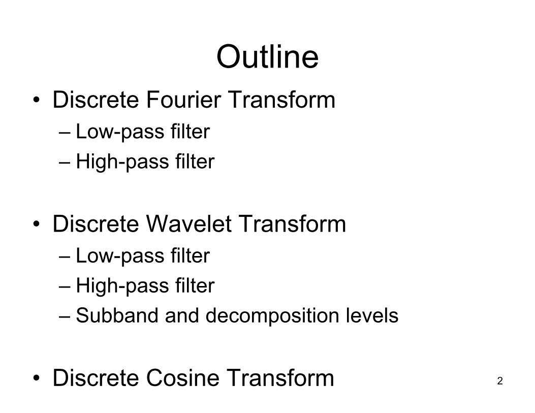
OutlineOutline• Discrete Fourier TransformDiscrete Fourier Transform

– Low-pass filterHi h filt– High-pass filter

• Discrete Wavelet Transform– Low-pass filter– Low-pass filter– High-pass filter– Subband and decomposition levels

2• Discrete Cosine Transform

Fourier TransformFourier Transform• Any function that is not periodic (but• Any function that is not periodic (but

whose area under the curve is finite) can b d th i t l f ibe expressed as the integral of sines and/or cosines multiplied by a weighting function.

• Images can be considered as functions of fi it d ti Th f th F ifinite duration. Therefore, the Fourier transform is the tool in which we are

3interested.

Perfect Reconstruction FeaturePerfect Reconstruction Feature• Fourier Transform has an important

h t i ti th t f ti d icharacteristic that a function expressed in a Fourier transform can be reconstructed (recovered) completely via an inverse process, with no loss of information.process, with no loss of information.

• This feature (Perfect Reconstruction Feature) allows us to work in the “Fourier )domain” and then return to the original domain of the function without losing any

4

domain of the function without losing any information.

2D Discrete Fourier Transformsc ete ou e a s oLet f(n,m) be a discrete 2D function resulted ( , )from uniformly sampling the continuous function f(x y) at intervals delta(x) andfunction f(x,y) at intervals delta(x) and delta(y). The DFT of f(n,m) is defined as:

∑∑−

+−−

=1

)//(21

)(1)(M

MvmNunjN

emnfvuF π∑∑==

=00

),(),(mn

emnfMN

vuF

where u =0, 1, 2, …, N-1 and v = 0, 1, 2, …, M-1.

5

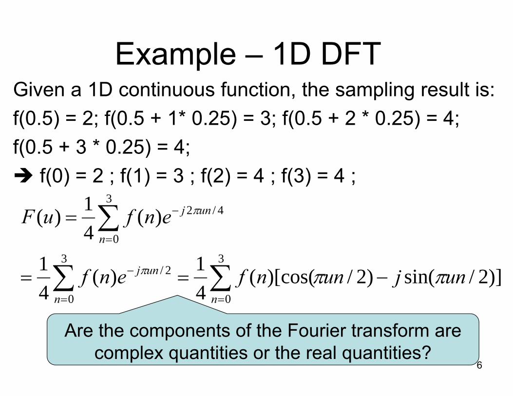
Example 1D DFTExample – 1D DFTGiven a 1D continuous function, the sampling result is:f(0.5) = 2; f(0.5 + 1* 0.25) = 3; f(0.5 + 2 * 0.25) = 4; f(0 5 + 3 * 0 25) = 4;f(0.5 + 3 0.25) 4;

f(0) = 2 ; f(1) = 3 ; f(2) = 4 ; f(3) = 4 ;1 3

)(41)(

3

0

4/2enfuFn

unj π= ∑=

−

)]2/sin()2/)[cos((41)(

41 3 3

2/ unjunnfenf unj πππ −== ∑ ∑−

Are the components of the Fourier transform are

44 0 0n n= =

6complex quantities or the real quantities?

413]4432[41]13121)1(10[410

//)* f( )* f( * f )*f(/ ) F(

=+++=+++=

]sin[cos1/41

413]4432[413 nπjnπf(n))F(

//

−=

=+++=

∑2]*4)1(*4)(*31*2[4/1

]2

sin2

[cos1/4 10

jjj

jf(n))F(n

+−

∑=

4]*4)1(*4)(*31*2[4/1

3

jjj =+−+−+=

]sin[cos)(4/1)2(0

njnnfFn

−= ∑=

ππ

]3i3)[(4/1)3(

4/1)]1(*41*4)1(*31*2[4/13 nnf

−=−++−+=

∑ ππ

2

]2

3sin2

3)[cos(4/1)3(0

j

njnnfFn

−= ∑=

ππ

74

2)](*4)1(*4*31*2[4/1 jjj −−=−+−++=

;4

2 1;4130 +−==

j)F(/ ) F(

.4

2)3(;4/1)2(

4−−

=−=jFF

11uhavewedomainfrequencyIn the

1/4;x have wedomain, spatial In the

==Δ

=Δ

Phase Magnitude, : thatmeansIt

1.xN

uhavewedomain,frequency In the =Δ

=Δ

o0,4/13;4/13)0()*00( ⇒==Δ+ FuF

o26,45;

42)1()*10( −⇒+−

==Δ+jFuF

o

52

0,4/1;4/1)2()*20( ⇒−==Δ+

j

FuF

8o26,

45.

42)3()*30( ⇒−−

==Δ+jFuF

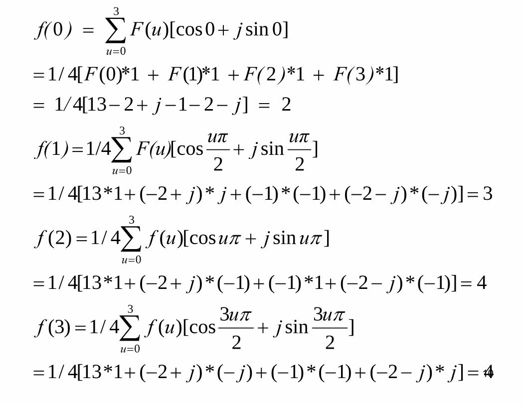
Inverse 1D DFTInverse 1D DFT• At a particular location n, f(n) can be p , ( )

reconstructed (or approximated) from the weighted sum of a basis function atweighted sum of a basis function at different frequencies (u = 0, 1, …, N-1). Th i ht i |F( )| th it d f• The weight is |F(u)|, the magnitude of a frequency component and the basis is sinusoid wave at different frequencies.

−1N

∑=

=0

/2)()(u

NunjeuFnf π

9

0u

]0sin0)[cos(03

0+= ∑

=

juF ) f(u

2]21213[41]13121)1(1)0([4/1

=+=+++=

jj/)* F( )*F( * F *F

]sin[cos1/41

2]21213[413

+=

=−−−+−=

∑ uπjuπF(u))f(

jj/

3)](*)2()1(*)1(*)2(1*13[4/1

]2

sin2

[cos1/4 10

=−−−+−−++−+=

+∑=

jjjj

jF(u))f(u

]sin[cos)(4/1)2(

)]()()()()([3

+= ∑ ujuuff

jjjj

ππ

4)]1(*)2(1*)1()1(*)2(1*13[4/10

=−−−+−+−+−+==

jju

]2

3sin2

3)[cos(4/1)3(3

0+= ∑

=

ujuuffu

ππ

104]*)2()1(*)1()(*)2(1*13[4/10

=−−+−−+−+−+==

jjjju

The following is the result obtained from using Matlab% A represents the 1D Discrete SignalA= [2 3 4 4] ;A [2 3 4 4] ;% Call the DFT of AB = fft(A)B = fft(A)B =13.0000 -2.0000 + 1.0000i -1.0000 -2.0000 - 1.0000i0000 0000 0000C = ifft(B)C =

What is the difference between our C =

2 3 4 4calculated result and Matlab’s result?

11

f(x) = 1 for x=0, 1, 2, …, 7; f(x) = 0 for x=8, 9, 10, …, 1023

Original Signal With Length of 1024 Its FT ResultOriginal Signal With Length of 1024 Its FT Result

12f(x) = 1 for x=0, 1, 2, …, 15; f(x) = 0 for x=16, 17, …, 1023

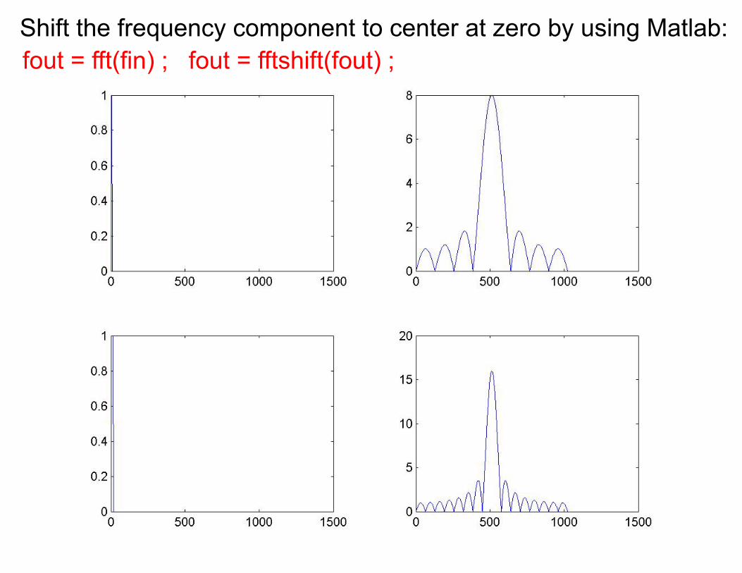
fout = fft(fin) ; fout = fftshift(fout) ;Shift the frequency component to center at zero by using Matlab:

13

2D DFT

),(),(),( vujIvuRvuF +=2D DFT can be represented by:

),(),(),( vujIvuRvuF +),(|),(|),( vujevuFvuF φ=

where |F(u,v)| is called Fourier spectrum of

|),(|),( evuFvuF

f(x,y) and Ф(u,v) is the phase spectrum. They are defined as:They are defined as:

5.022 )]()([|)(| vuIvuRvuF += )],(),([|),(| vuIvuRvuF +=),(t)( 1 vuI−φ

14),(),(tan),( 1

vuRvu =φ

A = [ 3 6 9 10 ; 2 4 9 0 ; 10 3 9 8 ; 20 4 8 14] ;Example – 2D DFT

A [ 3 6 9 10 ; 2 4 9 0 ; 10 3 9 8 ; 20 4 8 14] ;Results from 2D DFT by calling Matlab function: B = fft2(A)1 0e+002 *1.0e+002 1.19 0 + 0.15i 0.21 0 - 0.15i-0 02 + 0 31i -0 21 + 0 18i -0 12 + 0 03i 0 07 + 0 20i-0.02 + 0.31i -0.21 + 0.18i -0.12 + 0.03i 0.07 + 0.20i-0.03 -0.10 + 0.03i -0.13 -0.10 - 0.03i0 02 0 31i 0 07 0 20i 0 12 0 03i 0 21 0 18i-0.02 - 0.31i 0.07 - 0.20i -0.12 - 0.03i -0.21 - 0.18i

Center the frequency (0,0) by calling Matlab function: q y ( , ) y gfftshift(B)

1.0e+002 *-0.13 -0.10 - 0.03i -0.03 -0.10 + 0.03i-0.12 - 0.03i -0.21 - 0.18i -0.02 - 0.31i 0.07 - 0.20i

150.21 0 - 0.15i 1.19 0 + 0.15i-0.12 + 0.03i 0.07 + 0.20i -0.02 + 0.31i -0.21 + 0.18i

• The value of the transform at (u v) = (0 0)The value of the transform at (u, v) (0, 0) is:

∑∑−− 111 MN

∑∑==

=00

),(1)0,0(mn

mnfMN

F

• If f(x, y) is an image, the value of the Fourier transform at the origin is equal toFourier transform at the origin is equal to the average gray level of the image.

• F(0 0) is called dc (i e direct current)• F(0, 0) is called dc (i.e., direct current) component of the spectrum.

16

Some of the basis images used in a Fourier representation of an imagev p g

u

17

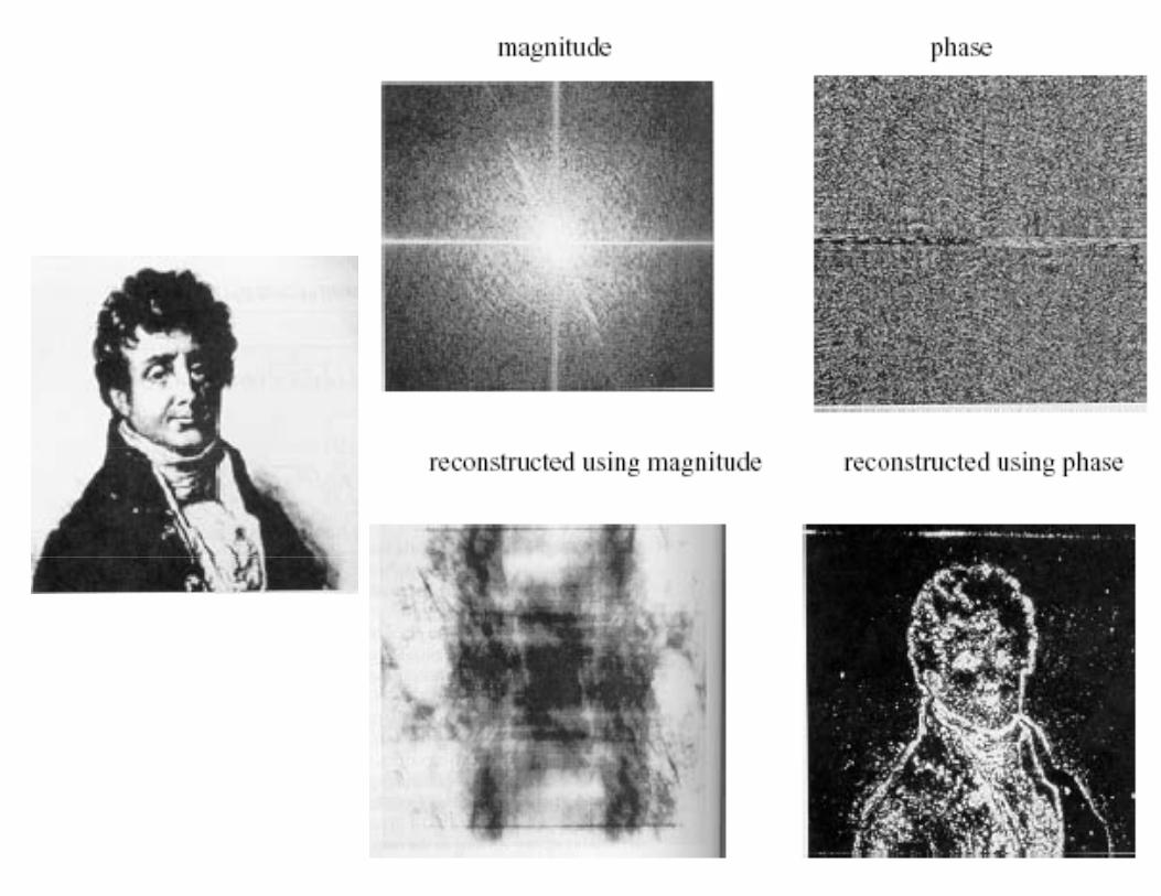
18

• Magnitude determines the contribution of each gsinusoidal component

• Phase determines where each of the sinusoidalPhase determines where each of the sinusoidal components resides. That is, it encodes the location of the frequency in the imagelocation of the frequency in the image.

• Without phase information, the spatial coherence of the image is disrupted and itcoherence of the image is disrupted and it becomes impossible to recognize feature of interest;interest;

• Without magnitude information, we can no l d t i th l ti b i ht f thlonger determine the relative brightness of those features, but we can at least see the boundaries b t th hi h id iti

19between them, which aids recognition.

Summary• An Image f in the Spatial Domain:1. (n, m) represents the spatial coordinates.2. f(n, m) represents intensity at (n, m).

• An Image f in the Frequency Domain:1. (u, v) is the spatial frequency that represents

intensity change with respect to spatial distance in a particular direction.

2 F( ) i d f th it d d h f2. F(u, v) is composed of the magnitude and phase of the spatial frequency at (u, v).

3 Low frequencies in the Fourier transform are3. Low frequencies in the Fourier transform are responsible for the general gray-level appearance of an image over smooth areas, while high frequencies

20

g , g qare responsible for detail, such as edges and noise.

Filtering and Enhancementi h F D iin the Frequency Domain

• FT transforms images from the spatial domain toFT transforms images from the spatial domain to the frequency domain.

• The usefulness of the FT• The usefulness of the FT– Remove undesirable frequencies from a signal

E i d f t t f t i ti i th– Easier and faster to perform certain operations in the frequency domain than in the spatial domain.

Enhancement in frequency domain is performed• Enhancement in frequency domain is performed via frequency filtering.

L filt i Att t hi h f i hil– Low-pass filtering: Attenuates high frequencies while “passing” low frequencies.High pass filtering: Attenuates low frequencies while

21

– High-pass filtering: Attenuates low frequencies while “passing” high frequencies.

The important point here is that the filtering process isThe important point here is that the filtering process is based on modifying the transform of an image in some way via a filter function and then taking the inverse of

22

way via a filter function, and then taking the inverse of the result to obtain the processed output image.

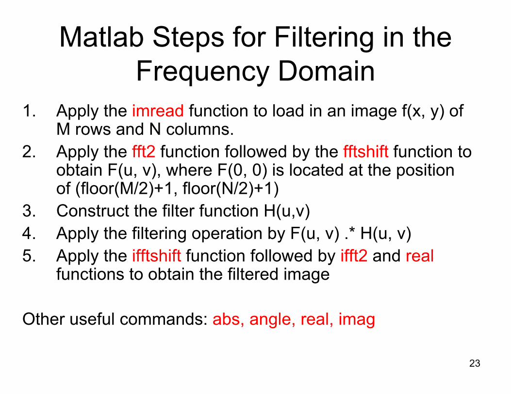
Matlab Steps for Filtering in the Frequency Domain

1. Apply the imread function to load in an image f(x, y) of M rows and N columns.

2 Apply the fft2 function followed by the fftshift function to2. Apply the fft2 function followed by the fftshift function to obtain F(u, v), where F(0, 0) is located at the position of (floor(M/2)+1, floor(N/2)+1)( ( ) ( ) )

3. Construct the filter function H(u,v)4. Apply the filtering operation by F(u, v) .* H(u, v)5. Apply the ifftshift function followed by ifft2 and real

functions to obtain the filtered image

Other useful commands: abs, angle, real, imag

23

The benefits of performing filtering in theThe benefits of performing filtering in thefrequency domain:q y

– It is convenient to perform a filter design. That is: Designing an appropriate filter to achieve theis: Designing an appropriate filter to achieve the given goal is convenient since filtering is more intuitive in the frequency domain.intuitive in the frequency domain.

– Implementation may be more efficient with FFT.Convolution in the spatial domain reduces to– Convolution in the spatial domain reduces to multiplication in the frequency domain, and vice versaversa.

24

25

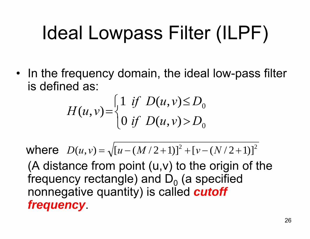
Ideal Lowpass Filter (ILPF)Ideal Lowpass Filter (ILPF)

• In the frequency domain, the ideal low-pass filter is defined as:

⎩⎨⎧

>≤

= 0

)(0),(1

),(DvuDifDvuDif

vuH

where

⎩ > 0),(0 DvuDif

22 )]12/([)]12/([)( +++ NMDwhere (A distance from point (u,v) to the origin of the frequency rectangle) and D (a specified

22 )]12/([)]12/([),( +−++−= NvMuvuD

frequency rectangle) and D0 (a specified nonnegative quantity) is called cutoff frequency

26

frequency.

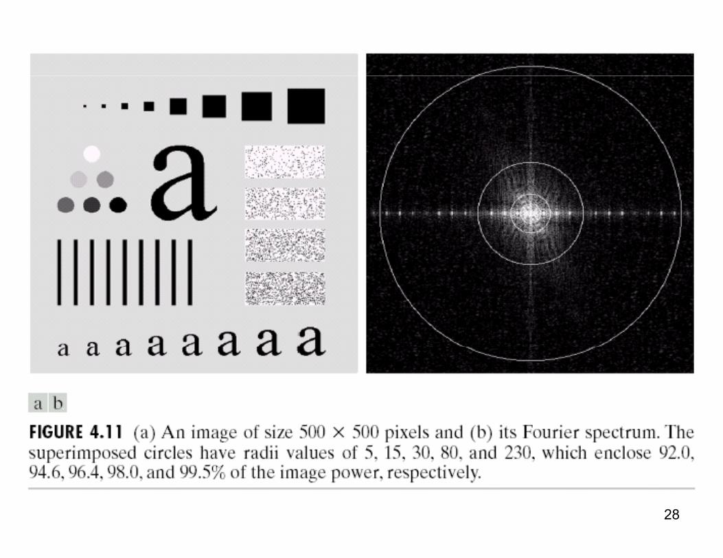
One way to establish a set of standard cutoff frequency loci is to compute circles that enclose

ifi d t f t t l i PTspecified amounts of total image power PT.

∑∑∑∑∑∑− −− −− − 1 1

221 1

21 1

))()((|)(|)(M NM NM N

IRFPP27

∑∑∑∑∑∑= == == =

+===0 0

22

0 0

2

0 0)),(),((|),(|),(

u vu vu vT vuIvuRvuFvuPP

28

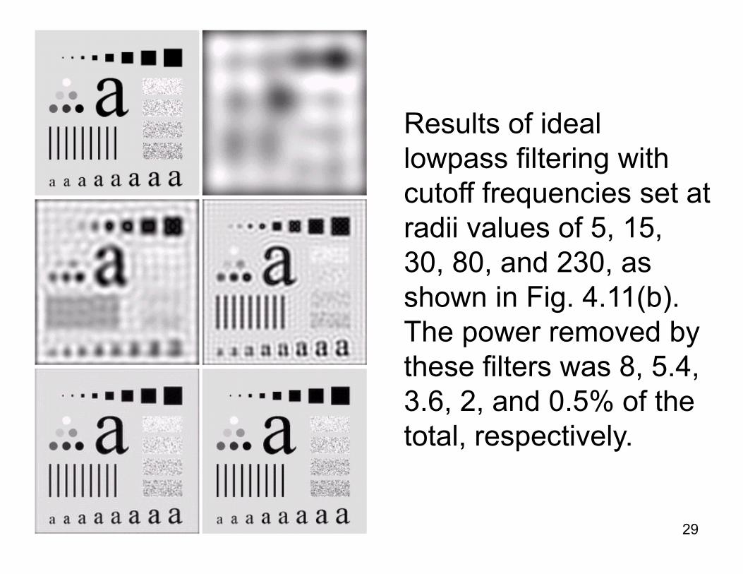
Results of ideal l filt i ithlowpass filtering with cutoff frequencies set at

dii l f 5 15radii values of 5, 15, 30, 80, and 230, as h i Fi 4 11(b)shown in Fig. 4.11(b).

The power removed by th filt 8 5 4these filters was 8, 5.4, 3.6, 2, and 0.5% of the t t l ti ltotal, respectively.

29

Butterworth Lowpass Filter (BLPF)Butterworth Lowpass Filter (BLPF)

• The transfer function of a Butterworth lowpass filter of order n, and with cutoff p ,frequency at a distance D0 from the origin, is defined as:is defined as:

H 1)( nDvuDvuH 2

0 ]/),([11),(

+=

where n is an integer. 30

• It does not have a sharp transition from passed and• It does not have a sharp transition from passed and filtered frequencies. Instead, it has a smooth transition.

• As n increases, the transition goes towards sharper.• In general, the order 2 is a good compromise

31

g , g pbetween effective lowpass filtering and acceptable ringing characteristics.

32

Results of ButterworthResults of Butterworth lowpass of order 2, filtering with cutofffiltering with cutoff frequencies set at radii values of 5 15 30 80values of 5, 15, 30, 80, and 230, as shown in Fig 4 11(b)Fig. 4.11(b).

There is no ringing effect due to the filter’s smooth transition between low and high frequencies.

33

Gaussian Lowpass Filter (GLPF)

Th i i f th d f th

20

222 2/),(2/),(),( DvuDvuD eevuH −− == σ

• The variance is a measure of the spread of the Gaussian curve. The larger the variance, the larger th t ff f d th ild th filt ithe cutoff frequency and the milder the filtering.

• No ringing in the case of GLPF.

34

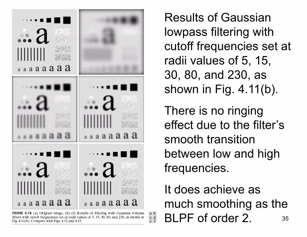
Results of Gaussian lowpass filtering withlowpass filtering with cutoff frequencies set at radii values of 5 15radii values of 5, 15, 30, 80, and 230, as shown in Fig 4 11(b)shown in Fig. 4.11(b).

There is no ringing effect due to the filter’s smooth transition between low and high frequencies.

It does achieve as much smoothing as the

35

much smoothing as the BLPF of order 2.

Sharpening Frequency Domain Filters

• Because edges and other abrupt changes in gray levels are associated with high-g y gfrequency components, image sharpening can be achieved in the frequency domaincan be achieved in the frequency domain by a highpass filtering process, which attenuates the low frequency componentsattenuates the low-frequency components without disturbing high-frequency information in the Fourier transform.

• Highpass Filter = 1 – Lowpass Filter36

Highpass Filter 1 Lowpass Filter

The Butterworth filter represents a transition between the sharpness of th id l filtthe ideal filter and the total smoothness ofsmoothness of the GaussianFilterFilter

37

38

39

Wavelet Transform• Wavelet coding is a type of image pyramid,

which is a powerful, but conceptually simplewhich is a powerful, but conceptually simple structure for representing images at more than one resolution. That is, image pyramid is a collection of decreasing resolution imagescollection of decreasing resolution images arranged in the shape of a pyramid.

• The basic idea is to represent a given functionThe basic idea is to represent a given function as a combination of "basis" functions belonging to a specified set, whose analytic properties are

dil ibl With l k th i f tireadily accessible. With luck, the given function is well approximated by just a few basis functions In that case it is easy to work with thefunctions. In that case, it is easy to work with the function. In particular, its description can be reduced from a painstaking point-by-point report t h df l f ffi i t

40to a handful of nonzero coefficients.

The level j-1 approximation output is used to create approximationThe level j 1 approximation output is used to create approximation pyramids, which contain one or more approximations of the original image.

41The level j prediction residual output is used to build prediction residual pyramids.

Approximation

Prediction Residuals

42

• In general a pyramid’s lower-resolution• In general, a pyramid s lower-resolution levels can be used for the analysis of large t t ll i t t itstructures or overall image context; its

high-resolution images are appropriate for analyzing individual object characteristics.

• Such a coarse to fine analysis strategy is ti l l f l i tt itiparticularly useful in pattern recognition.

43

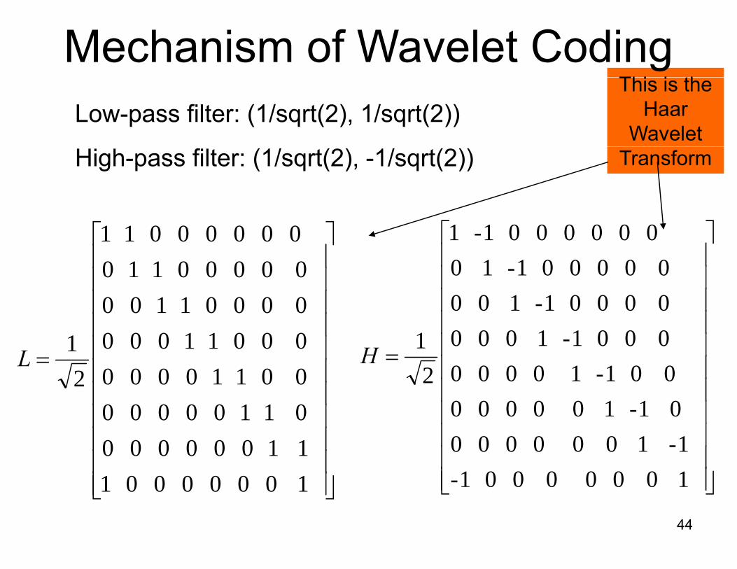
Thi i thMechanism of Wavelet Coding

This is the Haar

Wavelet Low-pass filter: (1/sqrt(2), 1/sqrt(2))

TransformHigh-pass filter: (1/sqrt(2), -1/sqrt(2))

⎥⎥⎤

⎢⎢⎡

0 0 0 0 0 1 1 00 0 0 0 0 0 1 1

⎥⎥⎤

⎢⎢⎡

0 0 0 0 0 1- 1 00 0 0 0 0 0 1- 1

⎥⎥⎥⎥

⎢⎢⎢⎢

0 0 0 1 1 0 0 00 0 0 0 1 1 0 0

1L ⎥⎥⎥⎥

⎢⎢⎢⎢

0 0 0 1- 1 0 0 00 0 0 0 1- 1 0 0

1H

⎥⎥⎥⎥

⎢⎢⎢⎢=

0 1 1 0 0 0 0 0 0 0 1 1 0 0 0 02

L

⎥⎥⎥⎥⎥

⎢⎢⎢⎢⎢=

0 1- 1 0 0 0 0 0 0 0 1- 1 0 0 0 02

H

⎥⎥⎥⎥

⎦⎢⎢⎢⎢

⎣ 1 0 0 0 0 0 0 1 1 1 0 0 0 0 0 0

⎥⎥⎥⎥

⎦⎢⎢⎢⎢

⎣ 1 0 0 0 0 0 0 1- 1- 1 0 0 0 0 0 0

44

⎥⎦⎢⎣ ⎦⎣

We can combine the filters in the following way to consolidate the low-pass and high-pass partsconsolidate the low pass and high pass parts.

Thus, the upper section in the result is the approximation, and the lower section in the result is the waveletand the lower section in the result is the wavelet (prediction residuals).

⎥⎥⎤

⎢⎢⎡

⎥⎥⎤

⎢⎢⎡

⎥⎥⎤

⎢⎢⎡

)1()0(

000011000 0 0 0 0 0 1 1

)2()0(

FF

GG

L

L

Low-

⎥⎥⎥

⎢⎢⎢

⎥⎥⎥

⎢⎢⎢

⎥⎥⎥

⎢⎢⎢

)3()2()1(

110000000 0 1 1 0 0 0 00 0 0 0 1 1 0 0

)6()4()2(

FFF

GGG

L

Lpass Filter

⎥⎥⎥⎥

⎢⎢⎢⎢

⎥⎥⎥⎥

⎢⎢⎢⎢

=⎥⎥⎥⎥

⎢⎢⎢⎢

)4()3(

0 0 0 0 0 0 1- 11 1 0 0 0 0 0 0

21

)0()6(

FF

GG

H

L

High

⎥⎥⎥⎥

⎢⎢⎢⎢

⎥⎥⎥⎥

⎢⎢⎢⎢

⎥⎥⎥⎥

⎢⎢⎢⎢

)6()5(

001-100000 0 0 0 1- 1 0 0

)4()2(

FF

GGH

High-pass Filter

45⎥⎥⎦⎢

⎢⎣⎥⎥⎦⎢

⎢⎣⎥

⎥⎦⎢

⎢⎣ )7(

)6(1- 1 0 0 0 0 0 00 0 1- 1 0 0 0 0

)6()4(

FF

GG

H

H

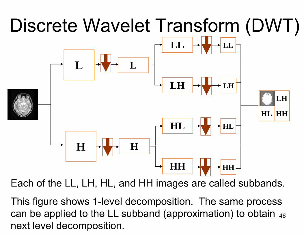
Discrete Wavelet Transform (DWT)sc ete a e et a s o ( )LL LL

L L

LH LH

LHLL

HL HH

LH

H H

HL HL

H H

HH HH

Each of the LL, LH, HL, and HH images are called subbands.

This figure shows 1-level decomposition The same process46

This figure shows 1-level decomposition. The same process can be applied to the LL subband (approximation) to obtain next level decomposition.

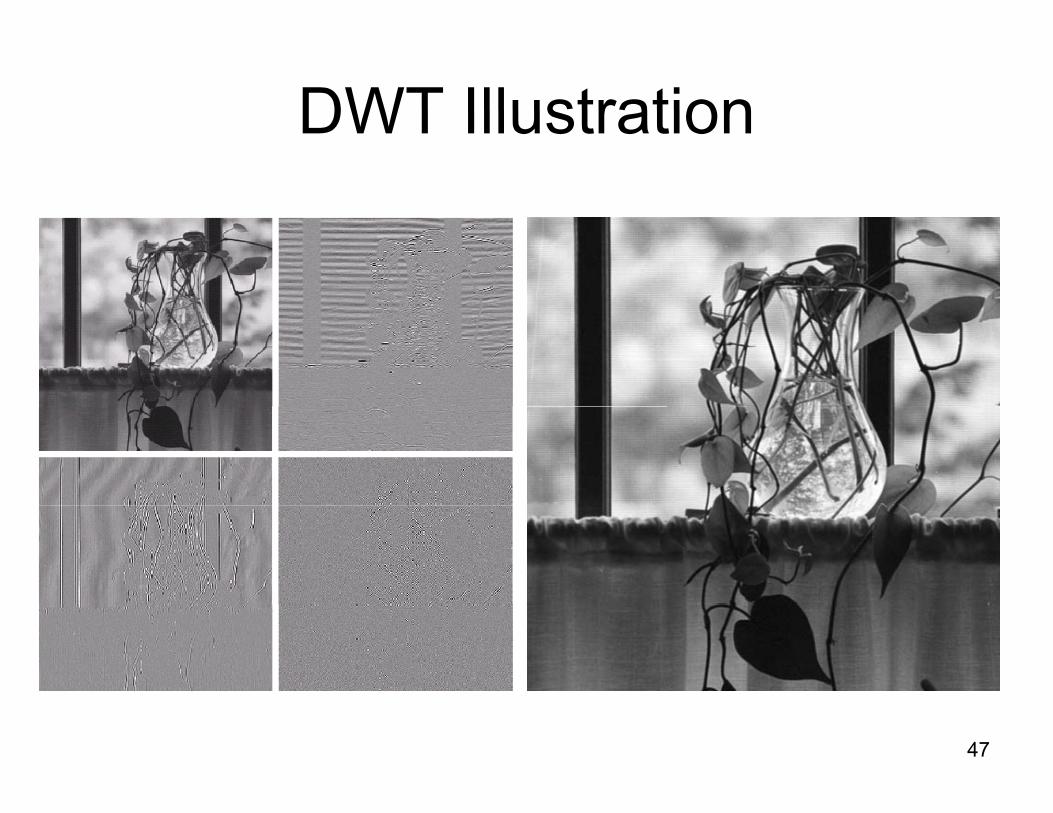
DWT IllustrationDWT Illustration

47

48

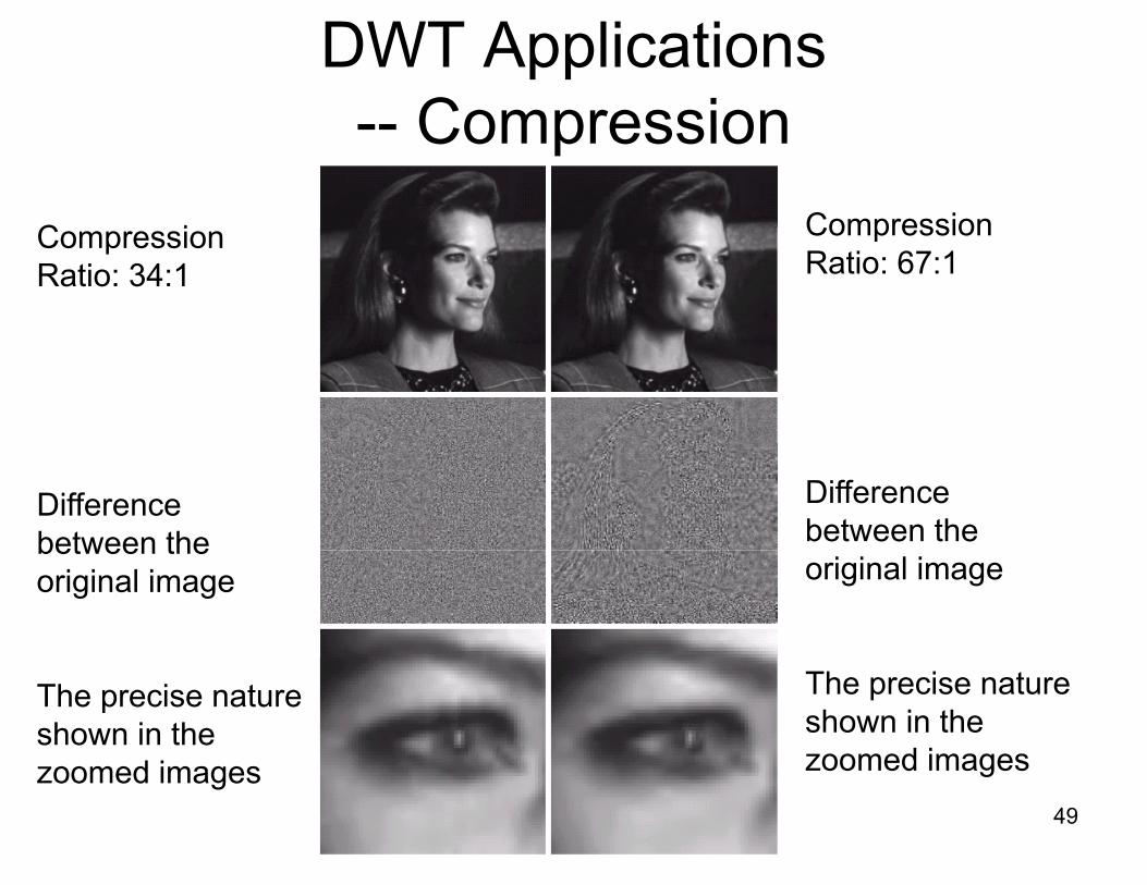
DWT ApplicationsCompression-- Compression

C i CompressionCompression Ratio: 34:1

Compression Ratio: 67:1

Difference between the

Difference between the between the

original image original image

The precise nature shown in the

d i

The precise nature shown in the zoomed images

49

zoomed images zoomed images

50

DWT ApplicationsDWT Applications• Noise Removal• Image/Video Retrieval

– Color– Texture– Shape

• Pattern Recognition– Medical Disease Diagnosis– Pedestrian Detection– Vehicle Detection

Di i l W ki• Digital Watermarking• Data Mining

51• Data Analysis

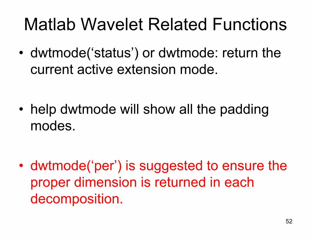
Matlab Wavelet Related Functions • dwtmode(‘status’) or dwtmode: return the

current active extension mode.

• help dwtmode will show all the padding modes.

• dwtmode(‘per’) is suggested to ensure the di i i t d i hproper dimension is returned in each

decomposition.52

• Practice on “wavemenu” command in Matlab• Type “help wavelet” in Matlab List all possible

wavelet related functions provided by Matlaba e e e a ed u c o s p o ded by a ab• “wavedec2” and “dwt2” are two functions used

for wavelet decomposition What is thefor wavelet decomposition What is the difference between these two functions?

• “waverec2” and “idwt2” are two functions used• waverec2 and idwt2 are two functions used for wavelet reconstruction. What is the difference between these two functions?difference between these two functions?

• Other useful commands: wfilters, waveinfo, fwavefun

• Common used wavelet filters: haar, db2, 53

biorthogonal

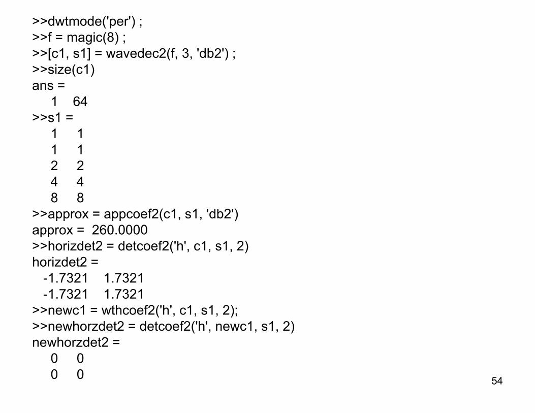
>>dwtmode('per') ;>>f = magic(8) ;>>[c1 s1] = wavedec2(f 3 'db2') ;>>[c1, s1] wavedec2(f, 3, db2 ) ;>>size(c1)ans =

1 64>>s1 =

1 11 12 24 48 8

>>approx = appcoef2(c1, s1, 'db2')approx = 260.0000>>horizdet2 = detcoef2('h', c1, s1, 2)horizdet2 =

-1.7321 1.7321-1.7321 1.7321

>> 1 th f2('h' 1 1 2)>>newc1 = wthcoef2('h', c1, s1, 2); >>newhorzdet2 = detcoef2('h', newc1, s1, 2)newhorzdet2 =

0 054

0 00 0

Practice Questions?Practice Questions?• What does the reconstruction image lookWhat does the reconstruction image look

like after the following operations:1) S t ll th i ti ffi i t1) Set all the approximation coefficients as

0’s2) Set the first level detail coefficients as 0’s3) Set the second level detail coefficients as3) Set the second level detail coefficients as

0’s4) How to get a refined approximation

incorporating only the 4-th level details?55

incorporating only the 4 th level details?

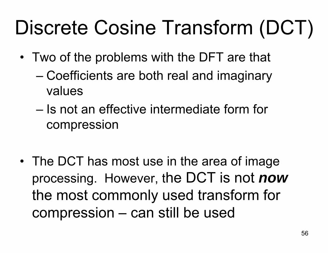
Discrete Cosine Transform (DCT)sc ete Cos e a s o ( C )• Two of the problems with the DFT are that

– Coefficients are both real and imaginary values

– Is not an effective intermediate form for compressioncompression

Th DCT h t i th f i• The DCT has most use in the area of image processing. However, the DCT is not nowthe most commonly used transform for compression – can still be used

56

p

x y are spatial coordinates in the samplex,y are spatial coordinates in the sample domain.u v are frequency coordinates in the transformu,v are frequency coordinates in the transform domain.

otherwisevCuCvuforvCuC

1)()(0,2/1)(),(

===

57

otherwisevCuC 1)(),( =

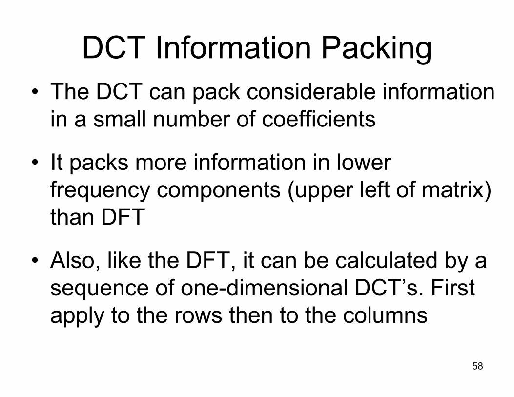
DCT Information PackingDCT Information Packing• The DCT can pack considerable information p

in a small number of coefficients

• It packs more information in lower frequency components (upper left of matrix) q y p ( pp )than DFT

• Also, like the DFT, it can be calculated by a sequence of one-dimensional DCT’s. Firstsequence of one dimensional DCT s. First apply to the rows then to the columns

58

DCT• The value in cell (1,1) is the “DC” value.

• Along row 1, only horizontal frequency components are presentcomponents are present.

Al l 1 l i l f• Along column 1, only vertical frequency components are present.

• The other row/columns contain varying amounts f b th h i t l d ti l f iof both horizontal and vertical frequencies.

59

Block DCToc C• An important feature of the DCT is that it has

l l tonly real components

• While the DCT can be applied to an entire image, it is normally applied (in JPEG) to small bl k f i 8 8 i l bl kblocks of an image, e.g., an 8x8 pixel block.

• Because for JPEG compression the DCT is done on 8x8 independent blocks, there tends to b bl ki i th i t hi h ibe blockiness in the image at high compression levels. The wavelet transform can overcome this problem

60

this problem

Useful Matlab CommandsUse u at ab Co a ds• fft2, fftshift, ifftshift, ifft2fft2, fftshift, ifftshift, ifft2• abs, angle, real, imag, log• wavedec2, dwt2 • waverec2 idwt2waverec2, idwt2• dwtmode• wfilters, waveinfo, wavefun• dct2 idct2• dct2, idct2

61