Basic Lessons in *ORA and Automap 2009casos.cs.cmu.edu/publications/papers/CMU-ISR-09-117.pdf ·...

Basic Lessons in *ORA and Automap 2009

Kathleen M. Carley, Mike Bigrigg, Jeff Reminga, John Storrick, Matt DeReno and Dave Columbus

July 2008 CMU-09-117

Institute for Software Research School of Computer Science Carnegie Mellon University

Pittsburgh, PA 15213

Center for the Computational Analysis of Social and Organizational Systems CASOS Technical Report1

1 This work was supported by the ONR N00014-06-1-0104, the AFOSR for “Computational Modeling of Cultural Dimensions in Adversary Organization (MURI)”, the ARL for Assessing C2 structures, the DOD, and the NSF IGERT 9972762 in CASOS. Additional support was provided by CASOS and ISRI at Carnegie Mellon University. The views and conclusions contained in this document are those of the authors and should not be interpreted as representing the official policies, either expressed or implied, of the National Science Foundation, the Department of Defense, and the Office of Naval Research, the Army Research Labs, the Air Force Office of Sponsored Research or the U.S. government.

ii

Key Words: DNA, ORA, Automap, Dynamic Network Analysis, MetaNetwork, Social Network Analysis

iii

Abstract ORA is a network analysis tool that detects risks or vulnerabilities of an organization’s design structure. The design structure of an organization is the relationship among its personnel, knowledge, resources, and tasks entities. These entities and relationships are represented by the Meta-Matrix. Measures that take as input a Meta-Matrix are used to analyze the structural properties of an organization for potential risk. ORA contains over 100 measures which are categorized by which type of risk they detect. Measures are also organized by input requirements and by output. ORA generates formatted reports viewable on screen or in log files, and reads and writes networks in multiple data formats to be interoperable with existing network analysis packages. In addition, it has tools for graphically visualizing Meta-Matrix data and for optimizing a network’s design structure. ORA uses a Java interface for ease of use, and a C++ computational backend. The current version ORA1.2 software is available on the CASOS website: http://www.casos.ece.cmu.edu/projects/ORA/index.html.

v

Table of Contents 1 Basic Lessons in *ORA .......................................................................................................... 1

Reports ............................................................................................................................................ 2

2 Belief Report ........................................................................................................................... 2

2.1 BELIEFS REPORT .......................................................................................................... 7

2.2 Analysis for the belief network: Agent x belief ............................................................... 8

3 Capacity Report .................................................................................................................... 11

3.1 Overall Capability and Needs ........................................................................................ 11

3.2 Highest Requirements .................................................................................................... 11

3.3 Requirements .................................................................................................................. 13

4..................................................................................................................................................... 13

5 Capacity Report .................................................................................................................... 14

5.1 Overall Capability and Needs ........................................................................................ 14

5.2 Requirements .................................................................................................................. 15

6 Key Entity Report — Basic .................................................................................................. 17

6.1 Main Dialog Box ............................................................................................................ 17

6.2 The Reports .................................................................................................................... 18

6.3 Output Options ............................................................................................................... 18

7 Key Entity Report — Other Options .................................................................................... 20

7.1 General Transformation ................................................................................................. 20

7.2 Remove Entities Options ................................................................................................ 22

7.3 Partition Options ............................................................................................................ 23

7.4 Summary ........................................................................................................................ 23

8 Mental Model Reports .......................................................................................................... 24

8.1 Mental Model Reports Bibliography .............................................................................. 24

9..................................................................................................................................................... 24

10 Tasks ..................................................................................................................................... 25

11 Contextual Menus ................................................................................................................. 25

12 Contextual Menus - Multi Files ............................................................................................ 27

13 Creating a Network from an Excel Spreadsheet ................................................................... 31

14 Hovering ............................................................................................................................... 33

15 Info Tab - Network ............................................................................................................... 34

16 Info Tab - NodeSet ................................................................................................................ 36

17 Running an Intelligence Report ............................................................................................ 37

17.1 Who are the critical actors? ........................................................................................ 37

17.2 INTELLIGENCE REPORT ....................................................................................... 39

17.3 KEY ACTORS ........................................................................................................... 39

17.4 Emergent Leader (cognitive demand) ........................................................................ 39

17.5 In-the-Know (total degree centrality) ......................................................................... 39

vi

17.6 Number of Cliques (clique count) .............................................................................. 40

17.7 Most Knowledge (row degree centrality) ................................................................... 40

17.8 Most Resources (row degree centrality) ..................................................................... 41

17.9 Leader of Strong Clique (eigenvector centrality) ....................................................... 41

17.10 Potentially Influential (betweenness centrality) ......................................................... 42

17.11 Connects Groups (high betweenness and low degree) ............................................... 42

17.12 Unique Task Assignment (task exclusivity) ............................................................... 43

17.13 Special Expertise (knowledge exclusivity) ................................................................. 43

17.14 Special Capability (resource exclusivity) ................................................................... 44

17.15 Workload (actual based on knowledge and resource) ................................................ 44

17.16 KEY KNOWLEDGE ................................................................................................. 45

17.17 KEY RESOURCES .................................................................................................... 45

17.18 KEY LOCATIONS .................................................................................................... 45

17.19 III. What do we know about an actor of interest? ...................................................... 48

17.20 1. Visualize information about a selected actor .......................................................... 48

17.21 2. Visualize an actor's sphere of influence ................................................................. 49

17.22 3. Run a Sphere of Influence Report .......................................................................... 50

17.23 SPHERE-OF-INFLUENCE REPORT ....................................................................... 51

17.24 Sphere of Influence Analysis for agent ahmed_ghailani ............................................ 51

17.25 Size Statistics .............................................................................................................. 51

17.26 Attributes .................................................................................................................... 52

17.27 Exclusive Connections ............................................................................................... 52

17.28 Most Similar Node...................................................................................................... 52

17.29 Top Measures ............................................................................................................. 52

17.30 Measure Value Range ................................................................................................. 53

17.31.......................................................................................................................................... 53

17.32 Resource Analysis Section ......................................................................................... 54

17.33 IV. What are the connections between two actors of interest? ................................... 55

17.34 V. What is the immediate impact of a particular agent on the network? ................... 56

17.35 VI. What happens to the network when certain entities are removed? ...................... 57

18 Create a New Meta-Network ................................................................................................ 65

18.1 Delete an existing node ............................................................................................... 66

18.2 Merge two nodes ........................................................................................................ 67

19 Performing a View Network Over-Time Analysis ............................................................... 67

19.1 Performing the Over-Time Analysis .......................................................................... 70

19.2 Example Slider Position 1 .......................................................................................... 71



19.5 WTC Event Node: Detail 1 - 1996 ............................................................................. 73

19.6 WTC Event Node: Detail 2 - 1997 ............................................................................. 74

19.7 Summary of Lesson .................................................................................................... 75

vii

20 Performing the View Measures Over-Time Analysis ........................................................... 76

20.1 Performing the View Measures Over-Time Analysis ................................................ 76

20.2 Interpreting The Results After Performing View Measures Over-Time Analysis ..... 77

21 Renaming .............................................................................................................................. 79

21.1 Renaming Meta-Networks, Meta-Nodes, and Networks ............................................ 79

22 Running An Over-Time Analysis ......................................................................................... 79

22.1 Overview: Over-Time Viewer .................................................................................... 79

23 Lessons .................................................................................................................................. 83

24 Lesson 1: ORA Overview ..................................................................................................... 83

24.1 Overview of ORA Interface ....................................................................................... 83

24.2 Loading a meta-network into ORA ............................................................................ 83

24.3 The Visualizer............................................................................................................. 84

25 Lesson 2: Creating A New Meta-Network ........................................................................... 86

25.1 Lesson - 101................................................................................................................ 86

25.2 lessons - 201-207 ........................................................................................................ 86

25.3 lessons - 301+ ............................................................................................................. 86

26 101 - Examine Your Data ..................................................................................................... 87

26.1 General Thoughts ....................................................................................................... 87

26.2 What's in a Node Class ............................................................................................... 88

26.3 Agents (Who) ............................................................................................................. 88

26.4 Locations (Where) ...................................................................................................... 90

26.5 Events (When) ............................................................................................................ 91

26.6 Tasks (How) ............................................................................................................... 91

26.7 Knowledge (What) ..................................................................................................... 92

26.8 Resources (What) ....................................................................................................... 92

26.9 Networks ..................................................................................................................... 93

26.10 Difference between the two MetaNetworks ............................................................... 93

27 201 - Excel and CSV............................................................................................................. 94

27.1 Your first NodeSet ...................................................................................................... 94

27.2 Your first Network...................................................................................................... 95

27.3 The rest of the NodeSets and Networks ..................................................................... 96

27.4 Saving as .CSV files ................................................................................................... 97

28 202 - Import into ORA .......................................................................................................... 98

28.1 Starting a new Meta-Network..................................................................................... 98

28.2 Adding to the new Meta-Network ............................................................................ 100

29 203 - Attributes ................................................................................................................... 103

29.1 The Special Attribute, "Title" ................................................................................... 103

29.2 Adding other Attributes and Values ......................................................................... 108

30 204 - Modifying a Meta-Network ....................................................................................... 110

30.1 Step 1: Adding a New Node ..................................................................................... 110

30.2 Step 2: Importing the Attributes ............................................................................... 113

viii

31 205 - Working with SubSets ............................................................................................... 115

32 206 - Attribute Columns ..................................................................................................... 117

32.1 Replacing an Attribute Column ................................................................................ 117

33 207 - Updating Your Data Files .......................................................................................... 119

33.1 Saving Your Network Data ...................................................................................... 119

33.2 Saving Your Attribute Data ...................................................................................... 120

34 301 - Import Analyst Notebook .......................................................................................... 122

35 Lesson 3: Key Entity Report ............................................................................................... 123

35.1 The Reports............................................................................................................... 123

35.2 Running a Key Entity Report: .................................................................................. 123

35.3 Remove Nodes from a Key Entity Report: ............................................................... 125

35.4 Comparison of the two reports ................................................................................. 129

35.5.......................................................................................................................................... 129

36 Lesson 5: Over-Time Analysis ........................................................................................... 130

36.1 Performing a View Network Over-Time Analysis ................................................... 130

36.2 Performing the Over-Time Analysis ........................................................................ 133

36.3 Example Slider Position 1 ........................................................................................ 134



36.6 WTC Event Node: Detail 1 - 1996 ........................................................................... 136

36.7 WTC Event Node: Detail 2 - 1997 ........................................................................... 136

36.8 Summary of Lesson .................................................................................................. 137

36.9 Performing the View Measures Over-Time Analysis .............................................. 137

36.10 Interpreting The Results After Performing View Measures Over-Time Analysis ... 139

36.11 Summary of Lesson .................................................................................................. 140

37 Lesson 8: Network Converter ............................................................................................. 142

37.1 Load Network ........................................................................................................... 142

37.2 Transform Network .................................................................................................. 142

37.3 Node Sets .................................................................................................................. 145

37.4 Nodes Add ................................................................................................................ 145

37.5 Nodes Delete............................................................................................................. 146

37.6 Nodes Merge............................................................................................................. 147

37.7 Node Properties ........................................................................................................ 149

37.8 Graphs ....................................................................................................................... 154

37.9 Save Networks .......................................................................................................... 154

38 Basic Lesson in Automap ................................................................................................... 155

38.1 Description................................................................................................................ 156

38.2 Concept List Procedure ............................................................................................ 156

38.3 Concept List Viewer functions ................................................................................. 157

38.4 Concept List and Stop Characters ............................................................................ 159

38.5 Description................................................................................................................ 160

ix

38.6 Delete List Procedure ............................................................................................... 160

38.7 Other Delete List Functions ...................................................................................... 162

38.8 Description................................................................................................................ 164

38.9 Thesauri Procedure ................................................................................................... 164

38.10 Thesauri Editor ......................................................................................................... 165

38.11 Questions regarding Thesauri ................................................................................... 165

38.12 Description................................................................................................................ 167

38.13 Procedure .................................................................................................................. 167

38.14 Description................................................................................................................ 172

38.15 Procedure .................................................................................................................. 172

38.16 Loading files into ORA ............................................................................................ 178

38.17 Display the Files ....................................................................................................... 179

38.18 ORA Reports ............................................................................................................ 180

38.19 Description................................................................................................................ 183

38.20 Description................................................................................................................ 186

38.21 PreProcessing Functions ........................................................................................... 187

38.22 Processing Functions ................................................................................................ 189

38.23 PostProcessing Functions ......................................................................................... 190

38.24 Running the Script .................................................................................................... 190

1

1 Basic Lessons in *ORA

2

Reports

2 Belief Report

Below are procedures to run a Belief Report in ORA. We set up an Excel spreadsheet with agents and the levels for each of the beliefs. Beliefs are strange as they can be either positive or negative. Two people share a belief only is both have a positive response or both have a negative response. From Excel, or other program you're using, save your data in the .csv format.

From the main menu select File => Data Import Wizard. Click the [Select] button to call up the open dialog box. Navigate to the directory where you have saved your .csv file.

3

Make sure the Create a New Matrix radio button is selected. Leave Choose a source node set set to agent. In the Choose a target node set click the down arrow to bring up the drop down menu. Highlight the <new type> option. Then select the Next button at the bottom of the box.

Type in belief into the textbox.

4

You can enter a new name in Enter a unique graph name or leave is as Agent x belief. When you're done, select the [Finish] button.

A new Network appears in Panel 1 with two Entites and one graph. The values from the Editor reflect the original numbers from the Excel spreadsheet.

5

Now you're ready to create a beliefs report. From the main menu select Analysis => Generate Reports.

1. In the Select Report textbox, select Beliefs. 2. In the Select one or more meta matrices: place a checkmark in the Networks you

want to run the report on. 3. In the Select the report formats to create: place a checkmark in all the formats you

want the final report to appear in. Here we are doing only Text (which will appear in panel 3 in the main interface) and HTML (which will create an HTML document that will open up in your browser.

4. In the Enter a filename section you can either type in a filepath or use the [Browse] button to navigate to a directory to save your files.

When you're finished select the [Next-->] button.

6

Select the Number of ranked nodes and critical attribute (if any). Then select the [Finish] button.

The Belief Report now appears in panel 3. If you selected HTML you will also see the report appear in your browser.

7

2.1 BELIEFS REPORT

Input data: Meta Matrix Start time: Wed Jul 25 21:24:34 2007 Given one or more belief networks, this analyzes the most strongly held beliefs, the most opinionated individuals and other characteristics of the belief networks. The beliefs node set must have the id equal to 'belief'. There can be multiple graphs based on this belief node set, for example, Agent x Belief and Organization x Belief.

8

2.2 Analysis for the belief network: Agent x belief 2.2.1 Most Common Beliefs Top 10 beliefs that are shared by the most people.

Belief Value Number of believers

Israel_is_a_state Negative 2

There_exists_a_Palestine_two_state_solution Negative 2

Hamas_should_PNA_elections Negative 2

Hamas_is_a_terrorist_organization Negative 3

Oslo_Accords_is_a_peace_solution Negative 3

Hamas_should_disarm Negative 3

Israel_should_Occupy_Palestine Negative 3

AB Positive 4

Hamas_is_a_terrorist_organization Positive 4

Hamas_should_government Negative 4

2.2.2 Most Contentious Beliefs Top 10 beliefs that are most disagreed upon across individuals. This is based on the GINI coefficient of the belief vector.

Belief Gini coefficient

AB 0.686667

Hamas_should_government 0.622222

Hamas_is_a_terrorist_organization 0.5625

Israel_should_Occupy_Palestine 0.5625

Oslo_Accords_is_a_peace_solution 0.456338

There_exists_a_Palestine_two_state_solution 0.454795

Hamas_should_PNA_elections 0.454795

Israel_should_Destruction 0.430818

Israel_is_a_state 0.37973

Hamas_should_disarm 0.270992

2.2.3

9

2.2.4 Most Strongly Held Beliefs Top 10 beliefs that are the most strongly held. This is the average absolute value of the belief vector.

Belief Score

Hamas_should_government 1.6

AB 1.5

Hamas_is_a_terrorist_organization 1.2

Israel_should_Occupy_Palestine 1.2

Israel_should_Destruction 0.97

There_exists_a_Palestine_two_state_solution 0.86

Hamas_should_PNA_elections 0.86

Oslo_Accords_is_a_peace_solution 0.84

Israel_is_a_state 0.78

Hamas_should_disarm 0.47

2.2.5 Most Likely to Change Beliefs Top 10 individuals most likely to change beliefs. This is based on the entropy of each individual's belief vector.

Belief Entropy

unknown-2 0

President George Bush 1

Condoleezza Rice 1.469

Ismail Haniya 1.65992

Bashar Al-Assad 2

Ehud Olmert 2.16578

Mahmud Abbas 2.19092

Khalid Mish?a 2.87598

Former President Carter 4.14443

unknown-1 4.2961

10

2.2.6 Most Opinionated Individuals Top 10 individuals that have the highest absolute sum of beliefs.

Agent Total beliefs

unknown-2 49.8

President George Bush 9.5

Bashar Al-Assad 9


Mahmud Abbas 8.6


Khalid Mish?a 4.9

unknown-1 3.2

Ismail Haniya 2.4

Ehud Olmert 1.6

2.2.7 Most Neutral Individuals Top 10 individuals that have the lowest absolute sum of beliefs.

Agent Total beliefs

Ehud Olmert 1.6

Ismail Haniya 2.4

unknown-1 3.2

Khalid Mish?a 4.9


Mahmud Abbas 8.6


Bashar Al-Assad 9

President George Bush 9.5

unknown-2 49.8

Produced by ORA developed at CASOS - Carnegie Mellon University

11

3 Capacity Report

The purpose of this report is to assess individuals' and organizations' capability to perform tasks. Below are procedures for running this report.

3.1 Overall Capability and Needs

List all congruence measures

1. For agents – list min, max, avg and std dev in capability for each capability index. 2. For organizations – list min, max, avg and std dev in capability for each capability

index 3. For tasks – list min, max, avg and std dec in requirements for each requirement

index

Most Capable List the top n most capable agents and next to their name list their capabilities (knowledge, resources, tasks).

NOTE : list overall capability first (don't show capabilities for the overall). List the top n most capable organizations and next to their name list their capabilities (knowledge, resources, tasks).

NOTE : List overall capability first, the overall explicit – then the three explicit. Then list the overall implicit and then the three implicit. NOTE : don't show capabilities for the overall measures.

3.2 Highest Requirements

List the top n tasks with the most requirements and next to each name list the requirements.

NOTE: list the overall first (don't show requirements for the overall). Capability Capabilities are defined in terms of expertise (knowledge) and resources.

NOTE : this formula discounts for the fact that most agents have some capabilities and assumes that there is a general discount to having large numbers of capabilities.

An agent's general capability index in resources is: ACR =1/(1+EXP(-((x-0.5)*10)))

Where x = number of resources the agent has divided by the maximum number of resources any agent has (so for AR this is the row sum divided by the max row sum)

An agent's general capability index in expertise is: ACK =1/(1+EXP(-((x-0.5)*10)))

12

Where x = number of knowledge the agent has divided by the maximum number of knowledge any agent has (so for AK this is the row sum divided by the max row sum)

An agent's capability can be inferred by the agent's experience. This is captured by the agent to task links. This is ACT=1/(1+EXP(-((x-0.5)*10))).

Where x = number of tasks the agent has divided by the maximum number of tasks any agent has (so for AT this is the row sum divided by the max row sum)

An agent's capability overall in both R, K and T is (ACR + ACK + ACT)/3 An organization's explicit capability is: An organization's general capability index in resources is: OCR =1/(1+EXP(-((x-0.5)*10)))

Where x = number of resources the organization has divided by the maximum number of resources any organization has (so for OR this is the row sum divided by the max row sum)

An organization's explicit capability index in expertise is: OCK =1/(1+EXP(-((x-0.5)*10)))

Where x = number of knowledge the organization has divided by the maximum number of knowledge any organization has (so for OK this is the row sum divided by the max row sum)

An organization's explicit inferred capability index using tasks is: OCK =1/(1+EXP(-((x-0.5)*10)))

Where x = number of tasks the organization has divided by the maximum number of tasks any organization has (so for OT this is the row sum divided by the max row sum)

An organization's overall explicit capability is (OCR + OCK + OCT)/3 An organization's implicit capability considers the expertise and resources of the agent's associated with the organization So this is for resources the average ACR across the agents associated with the organization. So this is for knowledge the average ACK across the agents associated with the organization. So this is for tasks (implicit inferred) the average ACT across the agents associated with the organization. From a network perspective, an agent is associated with an organization if AOij != 0. An organization's overall implicit capability is the sum of the 3 divided by 3. An organization's overall capability is the average of the explicit and implicit.

13

3.3 Requirements

Each task has requirements in terms of the knowledge and resources needed for that task.

Note : in practice it may not be possible to measure the requirements for all tasks, particularly for covert operations, prior to the task being done. So, a subject matter expert's view of the "complexity" of the task might be substituted. Such complexity would play the same role, and have the same properties as the requirements index defined here.

A task's general requirement index in resources is: RR =the number of resources needed for that task/maximum number of resources needed for any task (so for RT this is the col sum divided by the max col sum) A task's general requirement index in knowledge is: RK =the number of knowledge needed for that task / maximum number of knowledge needed for any task (so for KT this is the col sum divided by the max col sum) A task's overall requirement index is the average of RR and RK. Match In general agents with more capabilities when assigned to tasks with more requirements will better meet those needs. In general, agents with more capabilities will be able to perform more tasks. In general, tasks with higher requirements need either more agents or agents with more capabilities. When the exact requirements are done it is possible to do a match function. Here the idea is that the task is done best when the there is congruence between what resources/knowledge are needed for a task and what resources/knowledge those agents assigned to the task have. Several of the congruence measures in ORA apply here. For these definitions see the on-line ORA help.

4

14

5 Capacity Report

The purpose of this report is to assess individuals' and organizations' capability to perform tasks. Below are procedures to run a capacity report in ORA.

5.1 Overall Capability and Needs

List all congruence measures

1. For agents – list min, max, avg and std dev in capability for each capability index. 2. For organizations – list min, max, avg and std dev in capability for each capability

index 3. For tasks – list min, max, avg and std dec in requirements for each requirement

index

Most Capable List the top n most capable agents and next to name list their capabilities (knowledge, resources, tasks). Note; list overall capability first (don't show capabilities for the overall). List the top n most capable organizations and next to name list their capabilities (knowledge, resources, tasks). Note; list overall capability first, the overall explicit – then the 3 explicit, then the overall implicit and then the 3 implicit. Note, don't show capabilities for the overall measures. Highest Requirements List the top n tasks with the most requirements and next to each list the requirements. Note list the overall first (don't show requirements for the overall). Capability Capabilities are defined in terms of expertise (knowledge) and resources.

Note this formula discounts for the fact that most agents have some capabilities and assumes that there is a general discount to having large numbers of capabilities.

An agent's general capability index in resources is: ACR =1/(1+EXP(-((x-0.5)*10)))

Where x = number of resources the agent has divided by the maximum number of resources any agent has (so for AR this is the row sum divided by the max row sum)

An agent's general capability index in expertise is: ACK =1/(1+EXP(-((x-0.5)*10)))

Where x = number of knowledge the agent has divided by the maximum number of knowledge any agent has (so for AK this is the row sum divided by the max row sum)

An agent's capability can be inferred by the agent's experience. This is captured by the agent to task links. This is ACT=1/(1+EXP(-((x-0.5)*10))).

15

Where x = number of tasks the agent has divided by the maximum number of tasks any agent has (so for AT this is the row sum divided by the max row sum)

An agent's capability overall in both R, K and T is (ACR + ACK + ACT)/3 An organization's explicit capability is: An organization's general capability index in resources is: OCR =1/(1+EXP(-((x-0.5)*10)))

Where x = number of resources the organization has divided by the maximum number of resources any organization has (so for OR this is the row sum divided by the max row sum)

An organization's explicit capability index in expertise is: OCK =1/(1+EXP(-((x-0.5)*10)))

Where x = number of knowledge the organization has divided by the maximum number of knowledge any organization has (so for OK this is the row sum divided by the max row sum)

An organization's explicit inferred capability index using tasks is: OCK =1/(1+EXP(-((x-0.5)*10)))

Where x = number of tasks the organization has divided by the maximum number of tasks any organization has (so for OT this is the row sum divided by the max row sum)

An organization's overall explicit capability is (OCR + OCK + OCT)/3 An organization's implicit capability considers the expertise and resources of the agent's associated with the organization So this is for resources the average ACR across the agents associated with the organization. So this is for knowledge the average ACK across the agents associated with the organization. So this is for tasks (implicit inferred) the average ACT across the agents associated with the organization. From a network perspective, an agent is associated with an organization if AOij != 0. An organization's overall implicit capability is the sum of the 3 divided by 3. An organization's overall capability is the average of the explicit and implicit.

5.2 Requirements

Each task has requirements in terms of the knowledge and resources needed for that task.

16

Note, in practice it may not be possible to measure the requirements for all tasks, particularly for covert operations, prior to the task being done. So, a subject matter expert's view of the "complexity" of the task might be substituted. Such complexity would play the same role, and have the same properties as the requirements index defined here.

A task's general requirement index in resources is: RR =the number of resources needed for that task/maximum number of resources needed for any task (so for RT this is the col sum divided by the max col sum) A task's general requirement index in knowledge is: RK =the number of knowledge needed for that task / maximum number of knowledge needed for any task (so for KT this is the col sum divided by the max col sum) A task's overall requirement index is the average of RR and RK. Match In general agents with more capabilities when assigned to tasks with more requirements will better meet those needs. In general, agents with more capabilities will be able to perform more tasks. In general, tasks with higher requirements need either more agents or agents with more capabilities. When the exact requirements are done it is possible to do a match function. Here the idea is that the task is done best when the there is congruence between what resources/knowledge are needed for a task and what resources/knowledge those agents assigned to the task have. Several of the congruence measures in ORA apply here. For these definitions see the on-line ORA help.

17

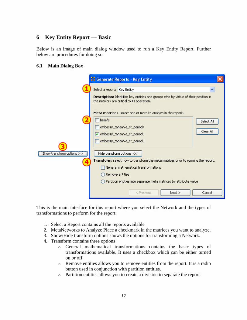
6 Key Entity Report — Basic

Below is an image of main dialog window used to run a Key Entity Report. Further below are procedures for doing so.

6.1 Main Dialog Box

This is the main interface for this report where you select the Network and the types of transformations to perform for the report.

1. Select a Report contains all the reports available 2. MetaNetworks to Analyze Place a checkmark in the matrices you want to analyze. 3. Show/Hide transform options shows the options for transforming a Network. 4. Transform contains three options

o General mathematical transformations contains the basic types of transformations available. It uses a checkbox which can be either turned on or off.

o Remove entities allows you to remove entities from the report. It is a radio button used in conjunction with partition entities.

o Partition entities allows you to create a division to separate the report.

18

6.2 The Reports

The Entity Report creates up to six separate reports.

1. KEY-ENTITY REPORT shows general information about the report 2. Who shows information about agents, such as Emmergent Leader, In the Know,

and Potential Influential. Gives information about knowledge that agents know, the resources they have access to, and what events the agents were at.

3. What shows information for tasks and the tasks related to agents, knowledge, etc. such as High Concentration of Actors, Knowledge, and Resources.

4. Where shows information about locations related to agents, resources, and tasks such as Central Locations, Most Active Locations, and Highest Concentration of Actors.

5. How shows information about the knowledge related to agents, knowledge, and loactions such as Dominant Knowledge, Most Available, Dominant Resources.

6. Performance Indicators shows information about Social Density, Communication, and Performance.

6.3 Output Options

You have a choice of four formats of report. Text places the reports in individual tabs in Panel 3 of the main interface. HTML creates reports that are opened up in a browser window. CSV are files that can be opened in Excel. And DyNetML creates .xml files, the default for ORA.

19

When you are finished, select [Finish].

20

7 Key Entity Report — Other Options

The Key Entities Report allows you to further tweak your report by defining parameters such as isolates, pendants, and binarizing your data. Following are three dialog boxes explaing those further refinements.

7.1 General Transformation

Occasionally your data needs work before creating the report. The General Transformation allows for refining it. See the dialog box below

• Remove Isolates: Remove any isolates* before running the report. • Remove Pendants: Remove any pendants* before running the report. • Symmetrize by method: Even out the matrix by using one of the methods i nthe

dropdown menu.

o Maximum : Acts like the binary OR function. If either one of a pair of nodes has a link then this function creates an equal link in the opposite direction.

o Minimum : Acts like the binary AND function. Both nodes need to have a link one another in order for a link to be valid. Else there is no link between the two nodes.

o Average :

21

• Remove links: Allows you to remove links from the report based on one of the options in the dropdown menu.

• Binarize: Binarizing* your numeric data will change all link weights to a value of either [1] or [0].

• Conform meta-matrice by method: • Create union matrices:

When you are finished, select [Next >].

22

7.2 Remove Entities Options

You can remove any of the nodes and stop them from affecting a report. By either using the tabs to find the entity in it's set or using the search box to single it out. Then place a checkmark in the box to remove it from view. The options are fairly self explanatory. You can create multiple filters with this method. The Filter Commands give you the choice of matching all or some of the filters you've created. And the [Reset Filters] button clears all the filters you've made. The filters can be refined by using the Search box to cal up particular nodes and marking them with a checkmark to remove them from the use. This can be done as many times as necessary before proceeding. You can also go through the tabs individually and choose to Select/Deselect whichever nodes you want. The [Select All] and [Clear All] buttons work on only the currently visible items. Any node that you place a checkmark in will be excluded from the filter. When you are finished, select [Next >].

23

7.3 Partition Options

From this screen choose an Entity from the top box. Place a checkmark in the appropriate checkbox. Next in the Select an attribute dropdown menu chose the attribute to base the report on. Finally chose and attribute value to use for the partition. If you want to create a new MetaMatrix place a checkmark in the bottom box add created partition meta matrices to the main interface. When you are finished, select [Next >].

7.4 Summary

With the Key Entities Report you can refine your report to focus on only the segment of your Network you prefer.

24

8 Mental Model Reports

What follows are descriptions of the various mental model reports in ORA. Single condensed files - per chunk, where a chunk is N days prior to or posterior to an event, excluding the day of the event Number of concepts - Number of words (frequency count per email) Carley and Kaufer, 1993 Number of isolated concepts - Number of words that were coded as knowledge items, but did not get linked into statements Carley and Kaufer, 1993 Number of statements - Number of links (frequency count per email) Carley and Kaufer, 1993 Density - Density of semantic network Carley and Kaufer, 1993 Set-Theoretic and qualitative (word-level) comparison of maps from before and after event Concept Analysis - Concepts are classified according to whether they have high and low values for the measures: total degree centrality, betweenness centrality, and consensus.

Allusions - high degree, low betweenness, low consensus Carley and Kaufer, 1993 Buzzwords - low degree, high betweenness, low consesus Carley and Kaufer, 1993 Emblems - low degree, high betweenness, high consensus Carley and Kaufer, 1993 Factoids - low degree, low betweenness, high consensus Carley and Kaufer, 1993 Ordinary Words - low degree, low betweenness, low consensus Carley and Kaufer, 1993 Placeholders - high degree, high betweenness, low consensus Carley and Kaufer, 1993 Stereotypes - high degree, low betweenness, high consensus Carley and Kaufer, 1993 Symbols - high degree, high betweenness, high consensus Carley and Kaufer, 1993

8.1 Mental Model Reports Bibliography

• Carley, Kathleen & Kaufer, David. (1993). Semantic Connectivity: An Approach for Analyzing Symbols in Semantic Networks. Communication Theory

• Wasserman, S., & Faust, K..

, 3, 183-213.

Social Network Analysis: Methods and Applications

•

. New York and Cambridge, ENG: Cambridge University Press.

9

Watts, D.J., Strogatz, S.H.(1998) Collective dynamics of 'small-world' networks. Nature 393:440-442.

25

10 Tasks 11 Contextual Menus

What follows are procedures for using ORA's contextual menus. Right-clicking on any Meta-Network, NodeSet, or Network brings up a contextual menu with the functions available with each.

The first four are self-explanatory. Transform… opens up the Meta-Network Transform… dialog box.

The first three are self-explanatory. Add Attribute … opens up the attribute function in order to add attributes to a nodeset.

26

The first two are self-explanatory.

• Set Diagonal… : Used on a square network to set cells 1,1 through x,x to the same value. In binary view the choise are 1: True (+1) 2: True (-1) 3: False (0). In Numeric view you can put any value into the diagonal.

• Fold Network… : This function creates a new network using matrix algebra. Below are four variations of a four x four network and the results when each is folded.

• Save Network… : Any Network can be saved individually to a file in one of the following formats: CSV*, DL, DyNetML*, or UNCINET (.##h). Also check File Formats for more information

• Binarize Network : Turns all non-zero numbers to [1] and leaving all [0] untouched.

• Remove Links… : Removes links in accordance to the selection in the dropdown menu (as seen in the images below).

• Symmetrize… :

27

12 Contextual Menus - Multi Files

There's also a separate contextual menu when you've got two or more Meta-Networks selected. Open up multiple Meta-Networks in the Main Interface. Load two or more files into Panel 1. We'll demonstrate this on two Meta-Networks containing Bob, Carol Ted, & Alice. The agents are identical but the tasks in each are different, except for driving which appears in both and has slightly different values. Inbetween the time of cookingIn and eatingOut Alice's feelings for Ted have grown. cookingIn and

eatingOut

28

Highlight both of them by holding down the [Control] while clicking on each file. Then Right-click on one of the files. This brings up the contextual menu.

The Add New MetaNetwork & Remove Selected Meta-Network are self-explanatory. The Union Meta-Network will create a new Meta-Network using one of five actions: sum, binary, average, minimum, or maximum.

• sum : In any identical network all values from all networks are added together. (i.e. bob's score of 4.0 in both meta-networks are added together for a total of 8.0).

• binary : Then in the binary option it doesn't matter what numbers appeared in either meta-network as it uses only 1 or 0 as a result. If any cell has a non-zero it will contain a 1 as a result.

29

• average : This option takes the sum of all identical cell values and divides them by the number of cells used. In cookingInted x alice contained a 2 while in eatingOut the value for tes x alice was a 1. This was averaged out to 1.5.

• minimum : This function finds the smallest value in any identical cells and uses that in the final result. (i.e. for ted x carol and ted x alice both cells use the smaller value of "1" even though they are from different meta-networks.

• maximum : This function finds the largest value in any identical cells and uses that in the final result. (i.e. for ted x carol and ted x alice both cells use the larger value of "2" and "3" respectively, each taken from a different meta-network.

Intersect Meta-Network works similar to the Union function and has the same five options. But in creating the new Meta-Network only nodes that appear in all Meta-Networks are carried over to the new Meta-Network. For example: All four agents appear in both Meta-Networks and are brought over into the new Meta-Network. But though there were six tasks in the cookingIn and three tasks in eatingOut there is only one task (driver) in the new Meta-Network created from the intersect function. Only nodes found in all Meta-Networks are brought over.

30

And even though bob has a value for driver in cookingIn only carol has a value for driver in both Meta-Networks.

Conform Meta-Network alters the selected Meta-Networks and makes them equal. union adds nodes that are found in one Meta-Network but not the other. inersect removes nodes that are not common to both.

31

13 Creating a Network from an Excel Spreadsheet

If you don't have a Network, you can create one from scratch. Below is step-by-step instruction on how to do this. We will create an square, agent-by-agent Network. We say it is square because all row headings correspond directly to column headings. This is important as it relates to specific measures ORA can run on a graph. If the graph is not square, some measures will not work. Open a blank Microsoft Excel work book. In column A we will enter the name of all the nodes that make up our social network or organization. 13.1.1 NOTE : When creating your spreadsheet, do not add any additional

titles, notes, or other headings, which will interfere with the "square" properties of the Network.

Next, create column headings using the correlating names as they appear in row headings. Again, this will ensure that our Network will be square.

Next we will create links between each agent. We do this by entering a 1 if a direct connection or relationship exists and a 0 if it does not. Please note that headings that cross-reference themselves are considered redundant and thus are left blank or 0. In the example below, Redundant cells are filled in with red strips to illustrate the self-loops. This redundancy should continue as a smooth diagonal line from the top left corner of your Network to the bottom right.

32

13.1.2 NOTE : If you don't end up with a diagonal line then your graph is not square.

Using 1s and 0s to establish link, complete your spreadsheet. In the Network example, we have assigned links randomly. Within your organization or network, however, you can describe any direct connections or relationships you are interested in analyzing. For instance, you may determine that a direct connection exists if agents within your network consult with each other at least once a month; literally, it can be anything you decide. Below is our completed Network (The red fill illustrates cells that do not require input due to their redundancy*).

Now that we have essentially built a Network from scratch using Excel, the next step is to save it in a compatible file format ORA can interpret. For Excel spreadsheets this will be the CSV* file format. 13.1.3 From the drop down menu: File => Save As Make sure you save this file as a CSV (comma delimited) You have now created a Network from scratch which can be loaded into ORA. Now return to ORA and load up your new Network. Below is a our new Network rendered in the ORA Visualizer. Notice the arrows only point from one node to another if there is a 1 in the column for a particular node. i.e. There is a "1" in the bob column for ted but a "0" in the ted column for bob. So an arrow points from ted to bob but NOT from bob to ted.

33

14 Hovering

Hovering the pointer over various parts of the panels will reveal information about the Meta-Network. Hovering over the parts in Panel 1 will reveal different information about the Meta-Networks, Meta-Nodes, and Networks.

34

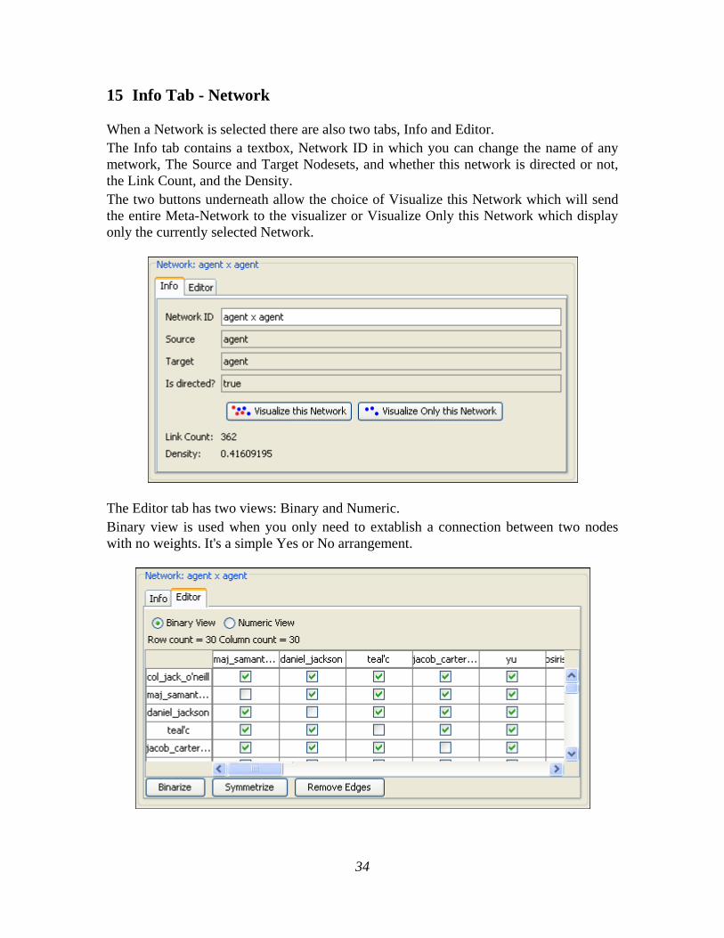
15 Info Tab - Network

When a Network is selected there are also two tabs, Info and Editor. The Info tab contains a textbox, Network ID in which you can change the name of any metwork, The Source and Target Nodesets, and whether this network is directed or not, the Link Count, and the Density. The two buttons underneath allow the choice of Visualize this Network which will send the entire Meta-Network to the visualizer or Visualize Only this Network which display only the currently selected Network.

The Editor tab has two views: Binary and Numeric. Binary view is used when you only need to extablish a connection between two nodes with no weights. It's a simple Yes or No arrangement.

35

The Numeric view allows you to treat links between various nodes with more or less importance. Notice that all the row nodes have a checkmarked connection to the column containing [yu] in the binary mode. This denotes they know one another. But in the numeric mode this value is a 0.5 which is used to denote previous acknowledgement but is an advesary.

36

16 Info Tab - NodeSet

Panel 2 contains two tabs, Info and Editor. The Info tab is mainly designed to display information regarding the Meta-Networks, NodeSets, and Networks. But this is the area where you can rename the Node Class ID and the Node Class Type. Place the cursor in the box, make sure the entire name is highlighted, and type in your new name. This area also gives you the Node Count of the selected Node Set as well as the Attribute Names contained within the NodeSet.

The Editor tab contains most of the editing functions.

1. The Search box for finding particular node(s) in a set. 2. The <set filter> for displaying only a particular sub-set of node(s). 3. The Checkboxes to designate which nodes to Delete or Merge. 4. The Nodes buttons: Create, Delete, Merge. 5. The Attributes buttons: Create and Delete.

37

17 Running an Intelligence Report 17.1 Who are the critical actors?

An Intelligence Report identifies key actors (individuals and groups) who are positioned in the network in ways that make them critical to its operation. To run an Intelligence Report:

• Return to the ORA interface. • Go to Analysis in the menu bar and click Generate Reports which brings up the

Generate Reports dialog box. • At the top of the window is a pull-down menu titled Select Report. Pull down the

menu by clicking the small inverted arrow icon to its right, and select Intelligence. • In the box titled Select one or more meta matrices: select the box for the Tanzania

Embassy bombing meta matrix. • At the bottom of the popup window is a file chooser titled Enter a file name (any

extension will be ignored) for the results file: Select the [Browse] button to the right and navigate to the location you want. Type in a filename (for example, IntelOutput) and select Open.

Below is a screen capture showing the popup windows with the correct options chosen:

• Select the [Next] button at the bottom of the dialog box. Select the [Finish] button.

38

An HTML file will pop up in your browser displaying the Intelligence Report. The same text is also displayed in Panel 3 in ORA. Below is a screen capture of the ORA interface with the Intelligence Report displayed in Panel 3:

39

Below is the HTML file for the Intelligence Report on the Tanzania Embassy bombing data:

17.2 INTELLIGENCE REPORT

Input data: TanzaniaEmbassyEnhance_2-07 Start time: Fri Feb 23 10:30:55 2007

17.3 KEY ACTORS 17.4 Emergent Leader (cognitive demand)

Measures the total amount of cognitive effort expended by each agent to do its tasks.

Rank Value Nodes

1 0.378917 fazul_mohammed

2 0.341104 khalfan_mohamed

3 0.299063 mohamed_owhali

4 0.280313 a13

5 0.269833 mohammed_odeh

6 0.243792 abdullah_ahmed_abdullah

7 0.192542 a10

8 0.183771 a4

9 0.180042 wadih_el-hage

10 0.176083 a16

17.5 In-the-Know (total degree centrality)

The Total Degree Centrality of a node is the normalized sum of its row and column degrees. Input graph(s): Agent x Agent

Rank Value Nodes

1 0.4 wadih_el-hage


3 0.266667 bin_laden


40

5 0.133333 ali_mohamed

6 0.133333 khalid_al-fawwaz

7 0.133333 a16

8 0.1 mohammed_odeh


10 0.0666667 a13

17.6 Number of Cliques (clique count)

The number of distinct cliques to which each node belongs. Input graph(s): Agent x Agent

Rank Value Nodes

1 2 wadih_el-hage

2 2 bin_laden

3 1 mohamed_owhali

4 1 ali_mohamed

5 1 khalid_al-fawwaz

6 1 abdullah_ahmed_abdullah

7 1 a16

8 0 khalfan_mohamed

9 0 mohammed_odeh

10 0 a4

17.7 Most Knowledge (row degree centrality)

The Row Degree Centrality of a node is its normalized out-degree. Input graph(s): Agent x Knowledge

Rank Value Nodes




41


5 0.5 wadih_el-hage

6 0.5 ali_mohamed

7 0.5 a10

8 0.5 jamal_al-fadl

9 0.5 a13

10 0.25 bin_laden

17.8 Most Resources (row degree centrality)

The Row Degree Centrality of a node is its normalized out-degree. Input graph(s): Agent x Resource

Rank Value Nodes



3 0.5 ahmed_ghailani




7 0.25 bin_laden

8 0.25 a10

9 0.25 a16

10 0 mohamed_owhali

17.9 Leader of Strong Clique (eigenvector centrality)

Calculates the principal eigenvector of the network. A node is central to the extent that its neighbors are central. Input graph(s): Agent x Agent

Rank Value Nodes



42



5 0.0992915 khalid_al-fawwaz



8 0.0583699 a16

9 0.0527998 mahmud_abouhalima


17.10 Potentially Influential (betweenness centrality)

The Betweenness Centrality of node v in a network is defined as: across all node pairs that have a shortest path containing v, the percentage that pass through v. Input graph(s): Agent x Agent

Rank Value Nodes






6 0 khalfan_mohamed

7 0 a4

8 0 fazul_mohammed

9 0 ali_mohamed

10 0 ahmed_ghailani

17.11 Connects Groups (high betweenness and low degree)

The ratio of betweenness to degree centrality; higher scores mean that a node is a potential boundary spanner. Input graph(s): Agent x Agent

Rank Value Nodes

43






6 0 khalfan_mohamed

7 0 a4

8 0 fazul_mohammed

9 0 ali_mohamed

10 0 ahmed_ghailani

17.12 Unique Task Assignment (task exclusivity)

Detects agents who exclusively perform tasks.

Rank Value Nodes Speciality

1 0.205078 fazul_mohammed t3

2 0.0136876 mohamed_owhali t1

3 0.0136876 a13 t1

4 0.011305 abdullah_ahmed_abdullah t1

5 0.00995741 ali_mohamed t1

6 0.00507781 khalfan_mohamed t5

7 0.00366313 a4 t5

8 0.00141468 mohammed_odeh t4

9 0.00141468 a16 t4

10 0.00134759 ahmed_ghailani t4

17.13 Special Expertise (knowledge exclusivity)

Detects agents who have singular knowledge.


1 0.0919699 bin_laden k4

44

2 0.0919699 khalid_al-fawwaz k4

3 0.00214043 mohamed_owhali k3

4 0.00214043 mohammed_odeh k3

5 0.00214043 fazul_mohammed k3

6 0.00191246 khalfan_mohamed k3

7 0.00191246 ali_mohamed k3

8 0.00168449 abdullah_ahmed_abdullah k3

9 0.000455941 wadih_el-hage k1, k2

10 0.000455941 a10 k1, k2

17.14 Special Capability (resource exclusivity)

Detects row nodes who have singular ties to column nodes. Input graph(s): Agent x Resource


1 0.108996 abdullah_ahmed_abdullah r4

2 0.0965488 ahmed_ghailani r4

3 0.0919699 bin_laden r2

4 0.0919699 a10 r2

5 0.0170257 fazul_mohammed r3

6 0.0124468 wadih_el-hage r3

7 0.0124468 a16 r3

8 0.00457891 khalfan_mohamed r1

9 0.00457891 mohammed_odeh r1

10 0 mohamed_owhali

17.15 Workload (actual based on knowledge and resource)

The knowledge and resources an agent uses to perform the tasks to which it is assigned.

Rank Value Nodes


45




5 0.230769 a13



8 0.153846 a16


10 0.0769231 ahmed_ghailani

17.16 KEY KNOWLEDGE

Dominant Knowledge (total degree centrality) The Total Degree Centrality of a node is the normalized sum of its row and column degrees.

Rank Value Nodes

1 0.571429 k2

2 0.428571 k1

3 0.333333 k3

4 0.0952381 k4

17.17 KEY RESOURCES

Dominant Resource (total degree centrality) The Total Degree Centrality of a node is the normalized sum of its row and column degrees.

Rank Value Nodes

1 0.333333 r3

2 0.285714 r1

3 0.190476 r4

4 0.142857 r2

17.18 KEY LOCATIONS

46

Dominant Location (total degree centrality) The Total Degree Centrality of a node is the normalized sum of its row and column degrees.

Rank Value Nodes

1 1.125 u_s

2 0.847222 afghanistan

3 0.833333 pakistan

4 0.722222 washington

5 0.708333 indonesia

6 0.701389 europe

7 0.673611 airport

8 0.604167 america

9 0.527778 turkey

10 0.506944 somalia

47

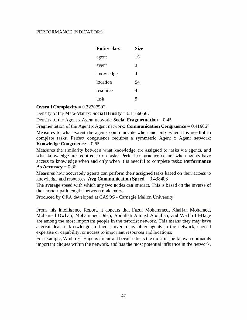
PERFORMANCE INDICATORS

Entity class Size

agent 16

event 3

knowledge 4

location 54

resource 4

task 5

Overall Complexity = 0.22707503 Density of the Meta-Matrix: Social Density = 0.11666667 Density of the Agent x Agent network: Social Fragmentation = 0.45 Fragmentation of the Agent x Agent network: Communication Congruence = 0.416667 Measures to what extent the agents communicate when and only when it is needful to complete tasks. Perfect congruence requires a symmetric Agent x Agent network: Knowledge Congruence = 0.55 Measures the similarity between what knowledge are assigned to tasks via agents, and what knowledge are required to do tasks. Perfect congruence occurs when agents have access to knowledge when and only when it is needful to complete tasks: Performance As Accuracy = 0.36 Measures how accurately agents can perform their assigned tasks based on their access to knowledge and resources: Avg Communication Speed = 0.438406 The average speed with which any two nodes can interact. This is based on the inverse of the shortest path lengths between node pairs. Produced by ORA developed at CASOS - Carnegie Mellon University

From this Intelligence Report, it appears that Fazul Mohammed, Khalfan Mohamed, Mohamed Owhali, Mohammed Odeh, Abdullah Ahmed Abdullah, and Wadih El-Hage are among the most important people in the terrorist network. This means they may have a great deal of knowledge, influence over many other agents in the network, special expertise or capability, or access to important resources and locations. For example, Wadih El-Hage is important because he is the most in-the-know, commands important cliques within the network, and has the most potential influence in the network.

48

17.19 III. What do we know about an actor of interest?

There are three ways to get additional information about an actor of interest:

17.20 1. Visualize information about a selected actor

For example, we can view information about Wadih El-Hage.

• Return to the meta matrix visualization pop-up window. • Single-click on the red circle for the actor of interest. A window will pop up

displaying information on the actor.

Below is a screen capture of the information resulting from clicking on the red circle for Wadih El-Hage:

49

17.21 2. Visualize an actor's sphere of influence

A sphere of influence is the set of actors, groups, knowledge, resources, events, and locations that influence and are influenced by a particular actor of interest. For example, we can examine the sphere of influence of Ahmed Ghailani. To visualize an actor's sphere of influence:

• Return to the meta matrix visualization pop-up window. • Make sure the whole meta matrix is visualized. If it isn't, go to Actions in the

menu bar and select Show All Entities. • Go to Tools in the menu bar and select Sphere of Influence. A window titled

Sphere of Influence (Ego Network) will pop up. • In the Search field halfway down the popup window, type the beginning of the

actor's name. From the options that appear in the chart below, click the box next to the name of your actor of interest. That actor's sphere of influence will be displayed in the visualization window.

Below is a visualization of the sphere of influence of Ahmed Ghailani:

To return to the original full meta matrix visualization, go to Actions in the menu bar and select Show All Entities.

50

17.22 3. Run a Sphere of Influence Report

A Sphere of Influence Report for an individual identifies the set of actors, groups, knowledge, resources, events, and locations that influence and are influenced by that actor. For example, we can examine the sphere of influence of Ahmed Ghailani. To run a Sphere of Influence Report:

• Return to the ORA interface. • Go to Analysis in the menu bar and click Generate Reports. A window titled

Generate Reports pops up. • At the top of the window is a pull-down menu titled Select Report. Pull down the

menu by clicking the small inverted arrow icon to its right, and select Sphere of Influence.

• In the box titled Select one or more meta matrices: click the box for the Tanzania Embassy bombing meta matrix.

• At the bottom of the popup window is a file chooser titled Enter a file name (any extension will be ignored) for the results file: Click the Browse button to the right and navigate to the location you want. Type in a filename (for example, SOIOutput) and click Open.

• Click the Next button at the very bottom of the popup window. • From the pull-down menu titled Select an Entity: choose Ahmed Ghailani. • Click the Finish button.

It may take a few minutes for ORA to run the Sphere of Influence Report. When ORA is finished, a small window will pop up tell you the analysis was successfully completed. Click OK. An HTML file displaying the Sphere of Influence Report will pop up in your browser window. Below is the HTML file for Ahmed Ghailani's sphere of influence:

51

17.23 SPHERE-OF-INFLUENCE REPORT

Input data: TanzaniaEmbassyEnhance_2-07 Start time: Fri Feb 23 11:10:54 2007

17.24 Sphere of Influence Analysis for agent ahmed_ghailani

The radius of the network is 1

17.25 Size Statistics

Contains the size of each node type within the ego network, expressed as an absolute value and as a percentage of the nodes in the original input network.

Node Type Size Percent

agent 1 +6%

manual_location 6 +11%

52

resource 2 +50%

task 1 +20%

17.26 Attributes

These are the attributes of the ego node.

Name Value

first_name ahmed

hostility_level 2

kinship mother

last_name ghailani

nationality tanzanian

nationality_relation hostile

nyi president

source_date 2006-05-10

source_name xmldata/pacrim_ilchul.xml

title ahmed_khalfan_ghailani

17.27 Exclusive Connections

Find nodes that have connections exclusively to the ego node. These are also called pendant nodes of the ego. There are no pendants attached to this node.

17.28 Most Similar Node

Computes the node that is most similar to the ego node with respect to Cognitive Similarity. This is computed two ways: first, using just the ego network, and second, using the original input network.

Network Node Type Node Name

Original Network agent abdullah_ahmed_abdullah

Ego Network agent ahmed_ghailani

17.29 Top Measures

53

Computes a collection of standard network analysis measures and reports those for which the ego node is among the top 10 nodes.

Measure Name Measure Input Rank Value

Centrality, Row Degree Agent x Resource 3 0.5

Centrality, Betweenness Agent x Agent 10 0

Boundary Spanner, Potential Agent x Agent 10 0

Exclusivity, Task Agent x Task 10 0.00134759

Exclusivity Agent x Resource 2 0.0965488

Actual Workload Agent x Knowledge 10 0.0769231

17.30 Measure Value Range

Computes a collection of network analysis routines for all the nodes in the network and reports whether the ego node has a Low, Medium, or High value with respect to the other nodes. Low means less than one standard deviation from the mean; high means more than one standard deviation from the mean; Medium is neither low nor high.

Measure Name Measure Input Range

Cognitive Demand Agent x Agent Medium

Centrality, Total Degree Medium

Clique Count Agent x Agent Medium

Centrality, Eigenvector Agent x Agent Low

Centrality, Betweenness Agent x Agent Medium

Boundary Spanner, Potential Agent x Agent Medium

Exclusivity, Task Agent x Task Medium

Exclusivity, Knowledge Agent x Knowledge Medium

Exclusivity Agent x Resource High

Actual Workload Agent x Knowledge Medium

17.31

54

17.32 Resource Analysis Section

Computes the resources that ahmed_ghailani can directly leverage and that can be mobilized. Direct resource are those directly connected to it, and indirect resources are those directly connected to a neighbor.

Resources that can be leveraged

Resources that can be mobilized ahmed_ghailani does not have any resources to mobilize.

Measure Value Percent of total

Direct resources 2 +50%

Indirect resources 0 0%

Possibly constrained resources 0 0%

Possibly constrained resources are both directly and indirectly linked to the ego entity. Contacts with the most resources (directly linked entities with the most resources):

Name Number of resources

Contacts with the unique resources (directly linked entities with exclusive resources):

Name Unique resources

Produced by ORA developed at CASOS - Carnegie Mellon University ________________________________________

55

17.33 IV. What are the connections between two actors of interest?

Sometimes, rather than influencing an actor directly, you may want to examine whether that actor has a connection with someone who is more interesting to you. For this, the Path Finder feature is most useful. For example, we can look at how Ahmed Ghailani and Wadih El-Hage are connected. To use the Path Finder feature:

• Return to the meta matrix visualization pop-up window. • Make sure the whole meta matrix is visualized. If it is not, go to Actions in the

menu bar and select Show All Entities. • Go to Tools in the menu bar and select Path Finder. A window titled Path Finder

will pop up. • In the bottom half of this pop-up window, there are two tabs titled Entity 1 and

Entity 2. Entity 1 is the from entity, and Entity 2 is the to entity. In other words, Path Finder searches for communication and information that is passed from Entity 1 to Entity 2.

• In the Entity 1 tab, type the name of your first actor of interest into the Search field. From the chart of agents below the Search field, check the box for the name of that agent. (For example, Ahmed Ghailani).

• Click on the Entity 2 tab and type in the name of your second actor of interest into the Search field. From the chart of agents below the Search field, check the box for the name of that agent. (For example, Wadih El-Hage).

• The visualization of the connections between Entity 1 and Entity 2 will appear in the visualization window.

56

Below is a screen capture showing the connection between Ahmed Ghailani and Wadih El-Hage:

17.34 V. What is the immediate impact of a particular agent on the network?

57

17.35 VI. What happens to the network when certain entities are removed?

We can examine the impact of removing a particular entity from the network by using Near Term Analysis (NTA). NTA removes a given entity and estimates the changes in the remaining network. This provides a what if?... analysis of the network. We can simulate strategic interventions or eliminations of certain agents, and examine how the network should react and change. For example, we can look at how the Tanzania Embassy bombing network changes if Ahmed Ghailani and/or Wadih El-Hage are eliminated. To run a Near Term Analysis: 1. Start the Near Term Analysis window

• Return to the ORA interface. • Make sure the meta matrix is highlighted in Panel 1. If it is not highlighted,

single-click on it. • Go to Analysis in the menu bar and select Near-Term Analysis. A window titled

Near Term Analysis will pop up.

NTA has two modes, Novice and Advanced, displayed as tabs in the Near Term Analysis pop-up window. Novice mode provides an automatic analysis set-up, but does not allow users to set up their own hypotheses.

• Click on the Advanced mode tab to switch to Advanced mode.

Below is a screen capture showing the Advanced mode tab in the Near Term Analysis pop-up window:

58

• In the field titled Settings, find the number boxes on the far right. Change the number of replications (the top number box) to 2, and the number of simulated time-points (the bottom number box) to 52. The timeline in the Simulated time line field will expand to include 52 time-steps.

2. Open the simulation scenario wizard

• In the middle of the pop-up window, find and click the Add new simulation instances button. A small window titled Near Term Analysis - Simulation scenario create wizard will pop up.

Below is a screen capture showing this wizard window:

• In this wizard window, make sure the first option in the Options field is selected. Click the Next button. The wizard window will display options for creating a custom scenario.

59

Below is a screen capture showing this custom scenario field in the wizard window:

3. Remove Wadih El-Hage

• Click the box for Wadih El-Hage in the table of agents in the wizard window. Change the Timing box to 10 in the same row.

• To add this event set-up to the Near Term Analysis, click the Add events button located next to the Search field (above the list of agents).

The timeline at the top of the wizard window will mark the isolation of Wadih El-Hage at time 10.

60

Below is a screen capture of this timeline:

• Click the Add a simulation button at the bottom of the wizard window. The wizard window will close automatically. In the NTA window, the new simulation case will appear in the Cases to simulate field.

4. Remove Ahmed Ghailani

• Follow Step 3, but replace Wadih El-Hage with Ahmed Ghailani.

Your two simulation cases appear in the Near Term Analysis window in the Cases to simulate field, along with the Baseline case. The Baseline case is simply the network with no entities removed. You can view your different simulation cases by clicking on them in the Cases to simulate field, and the simulation time-line will change accordingly. 5. Run the Near Term Analysis

• Click the Execution button at the bottom of the Near Term Analysis window. • A small window will pop up to warn you that the execution may take a long time.

Click OK. Another small window will pop up to show you how the simulations are progressing in the Near Term Analysis.

6. View the results of the Near Term Analysis

• When the analysis is complete, a new window titled Near Term Analysis Results will pop up.

61

Below is a screen capture of the results pop-up window:

These two performance lines correspond to deviations from the baseline of knowledge diffusion over time. Examining this performance change over time reveals how much an agent's elimination impacts the performance of the organization.

• To draw a bar chart, click the Draw bar chart button in the results window. The resulting bar chart displays a performance comparison for each time-point.

62

Below is a screen capture of the bar chart:

The results of the Near Term Analysis are also available in HTML format. 7. Save the results of the Near Term Analysis in HTML format

• Go to File in the menu bar and select Save the html report. A file chooser window will pop up. Navigate to the location you want and type a filename for your HTML report.

• A window titled Image Size Input will pop up. Type in the width of the image and click OK.

• Another window titled Project Saved will pop up displaying the location of your saved analysis results. Click OK.

8. Save the organizational structures resulting from your simulations in ORA

• Return to the ORA interface. • To save the Agent-to-Agent communication network at time-step 40 in the

simulation, go to File and select Save the Agent-to-Agent communication matrices during evolution.

• A small window titled Save the probability of interaction matrix will pop up. Click the Yes button.

• Another small window titled Save timing will pop up. Enter 40 and click OK. • A final window titled Saved will pop up. Click OK.

63

You can view saved simulations in Panel 1 of the ORA interface.

64

Below is a screen capture of Panel 1 after simulations have been saved:

65

18 Create a New Meta-Network

There are times you need to run measures on or visualize only part of an existing Meta-Network. This section will show you the easy way to create sub-sets of an existing Meta-Network. First duplicate the Meta-Network. Highlight the Meta-Network then from the main menu select Edit => Copy Meta-Network. Then form the main menu select Edit => Paste Meta-Networks. It would be a good idea to rename this new Meta-Network immediately so as to not get it comfused with the original. Next, expand the Meta-Network you want by clicking the [+] if it isn't expanded already. Highlight the nodeset with the nodes you want to remove.

In panel 2 select the Editor tab which brings up the matrix with nodes on the vertical and attributes on the horizontal. Below each attribute is a <set filter>. Below left is the stargate_summit meta-network along with the ally attribute. I wish to make a new meta-network of the good guys only. In the dropdown menu under ally I select no. These are the nodes I want to remove.

Place a checkmark in the box of each node. Below the matrix under Nodes are three buttons. Click the [Delete] button. The new nodeset now contains only the nodes that had yes in the attribute ally.

66

With this same procedure I created a Meta-Network of only the bag guys.

Creating or Deleting Nodes Creating a new Node What follows are procedures for creating a new node in your dataset. Highlight a NodeSet where the node is to be added. Click [Create].

You will be prompted to input the number of new nodes you want to create in the NodeSet. Input the number of nodes to add and select [OK] and the new node(s) will appear at the bottom of the nodeset.

The new node can then be renamed by clicking inside the cell.

18.1 Delete an existing node

To delete a node from a NodeSet place a checkmark in the box(es) to the left of the node(s) and select [Delete].

Select [OK] and all nodes with checkmarks will be deleted from the NodeSet.

67

18.2 Merge two nodes

The Merge button combines the links and attributes of the selected nodes and creates a merged or combined node. The nodes that were merged are removed, and replaced with the combined node. Used primarily when data needs to be consolidated.

Example: You have two nodes, Bob and Robert. They are actually the same node and you want to combine their information into one node.

19 Performing a View Network Over-Time Analysis

The purpose of this lesson is to perform both a View Network Over Time and View Measures Over Time Analysis. To do so requires multiple network datasets representative of your network over different times. The goal is to analyze how a network changes across multiple times. The period is determined by the intervals of collected network data and presented as multiple Meta-Matrices, which are loaded into ORA in sequential order. The steps below provide detailed instruction on how type of analysis. To perform a View Network Over-Time Analysis, you must load Meta-Matrices that relate to different time captures of your network data, which need to be in the form of multiple Meta-Matrices. In the following example, we will use network time captures of the 1998 Embassy Bombing in Tanzania Meta-Matrix data set and compare the same data set as we knew it in 1997 and 1996 and 1998. We will then compare all the Meta-Matrices in the Network Over-Time Viewer to gain a visual representation of how this network changed between 1996 and 1998. NOTE : For our purposes, we have changed data in this example and have renamed the Meta-matrix for three different years. This will denote different network variables that have changed over time. You will see in the left windowpane under input dataset three Meta-Matrices, 1998, 1997, and 1996, have been loaded.

68

From the main menu, select File => Open Meta Matrix

Choose [Select Files]

69

You will see all of our example data sets, which will load simultaneously into ORA, buy highlighting and selected all the files. Highlight all files you analyze in Over-Time Viewer. Press [Enter].

The import data window will appear (below). This will confirm the files you wish to analyze.

Select [Finish].

70

All three Meta-Matrices should display in Panel 1.

19.1 Performing the Over-Time Analysis

Now that we have time captures of our network data represented and loaded into ORA in the form of three Meta-Matrices relating to 1996, 1997 and 1998, we can perform the Over-Time Analysis. 19.1.1.1 From the Menu Bar => Data Visualization => View

Network Over-Time

The ORA Visualizer will render all of the loaded Meta-Matrices. Please take special note of the Time Viewer pop-up Window. This window displays a slider, which will allow you to quickly change from the first Meta-Matrix time capture of 1996, to 1997 and 1998 respectively.

71

By moving the slider from one Meta-Matrix to the next, you will gain a visual perspective on how the network has changed over Time. The series of screen shots below display how the visualized data changes from one slider to position to the next. These renders then allow you a picture of how the network changes Over-Time. NOTE : Depending on the complexity of the network and the extent to which relationships (ties) have changed, the visualization of those changes may be subtle. The screen shots below, however, will emphasize the extent to which the role of the WTC Event node has changed from 1996 to 1998 in relation to the network of which it is part of namely the Tanzania data set. Below these screen captures, are a series of detail screen captures focusing on the WTC Event node.

19.2 Example Slider Position 1

72



73

Detail of WTC Event Node when visualized in the Over-Time Viewer as part of the 1996, 1997 and 1998 Tanzania Data Sets.

19.5 WTC Event Node: Detail 1 - 1996

74

19.6 WTC Event Node: Detail 2 - 1997 19.6.1.1 Notice who how the relationships of this node to the rest

of the network has changed from 1996 to 1997.

19.6.1.2 Notice that the connections (links) have changed from 1996 to 1997.

75

As you can see, as we progress through the data sets pertaining to 1996, 1997 and 1998, the event node WTC lost direct ties to other parts of the network. In the 1996 data set, WTC had 3 ties to other nodes in the Tanzania Embassy network; In 1997, only 2; Finally, in 1998, the WTC event node had only 1 link to Tanzania Network. This may indicate that the WTC node may have lost importance from one year to the next.

19.7 Summary of Lesson

At this point, you should be able to complete the following tasks to perform an Over-Time Network Analysis.

• Load multiple Time Data Captures in the form of Meta-Matrices, which are representative of your network (Meta-Matrix) over time.

• Use the Over-Time slider window tool to move from one time capture to the next. • Gain a visual perspective of how your overall network has changed from one time

capture to the next.

76

20 Performing the View Measures Over-Time Analysis

ORA provides an alternative method to analyzing your network data (in the form of MetaNetworks captured over time) than the only in the Visualizer. By running a View Measures Over Time analysis you can visualize how your network changes in relation to any given measure in the form of charts, which take you from one time point to the next. Below is a series of screen captures and instruction on how to access the View Measures Over Time feature: From the main menu bar select Data Visualization => View Measures Over Time

20.1 Performing the View Measures Over-Time Analysis

ORA provides an alternative method to analyzing your network data (in the form of MetaNetworks captured over time) than the only in the Visualizer. By running a View Measures Over Time analysis you can visualize how your network changes in relation to any given measure in the form of charts, which take you from one time point to the next. Below is a series of screen captures and instruction on how to access the View Measures Over Time feature: 20.1.1.1 From the main menu bar: Data Visualization => View

Measures Over Time

Select View Measures Over Time.

Select [OK]

77

The View Measure Over Time Window will appear. You will see that this window is primarily organized into three sections. Area 1: is a slider where you can control various inputs that affect the aggregation level of your Meta Matrices. Area 2: is a tabbed index allowing you to select the graph level you desire and the individual node sets you are interested in analyzing. Area 3: displays the actual chart based on the measures you selected in the tabbed index and the position of the aggregation slider.

20.2 Interpreting The Results After Performing View Measures Over-Time Analysis

In the example above, we have loaded all three of our network time captures into the View Measures Over Time Analysis tool. The result of our analysis, as we have indicated before, will be displayed as a chart in the bottom section of the ORA interface in Panel 3. But, what does this tell us? To find out, we will examine the Graph Level measure Knowledge Waste. From the tabbed measures window: 20.2.1.1 Graph tab > Congruence, Organization Measure,

Knowledge Waste.

78

The result is displayed below.

We can see the chart displays an axis scale correlating to our networks over time. The graph level measure of Knowledge Waste was selected using the View Measures Over Time tool and the result is displayed in the chart area of the window. We can see that the graph level measure of Knowledge Waste held a value slightly above 40 in the first Meta Matrix, 1996, displayed with 1 on the Time axis. We can deduce from the chart that in 1997 something affected our measure of Knowledge Waste to increase the value to nearly 60. This corresponds to the time scale axis of 2, which represents 1997, our second year of network data. In the final year, 1998, our measure of Knowledge Waste declined to the value in 1996. This should be visually evident with its relative line graph position. It is clear that the value for the Knowledge Waste Measure increased from the first Meta Matrix (1996) to the second (1997) and then retreated back to its original (1996) level. It would be up to you to determine what may have affected that measure for it to undergo this progression and regression.

Summary of Lesson At this point, you should be able to complete the following tasks to perform a View Measures Over-Time Analysis:

• Load multiple data files into ORA (in the form of Meta-Matrices) representative of your network across certain periods.

• Select an aggregation level and choose a graph level or node level set to analyze. • Analyze the data output in the charting tool located in the bottom section of the

View Measures Over Time window.

79

• See how your network may have changed from one time capture to the next for any given graph level or entity node measure.

• Use this visual comprehension to draw conclusions about how your network changed across multiple times.

21 Renaming 21.1 Renaming Meta-Networks, Meta-Nodes, and Networks

ORA allows you to rename the Meta-Network, Meta-Node, and Networks. This helps makes the information clearer for you. Below I renamed one of the Meta-Nodes to those guys and also renamed the type to who?. You can see how it's reflected throughout the entirely of panel 1. So you can rename any Meta-Node in a Meta-Network for better readability.

22 Running An Over-Time Analysis 22.1 Overview: Over-Time Viewer

To run the Over-Time Viewer, you must first load MetaNetworks that relate to different time captures of network data. In the example below, you will see in the left window pane under input dataset three MetaNetworks, 2000, 2001, and 2002, have been loaded. Once you have loaded your MetaNetworks, select the Over-Time Viewer from the main interface tool bar under Data Visualization. The black ellipse in the screen shot below illustrates how to access the Over-Time Viewer from ORA's main interface.

80

From the drop-down menu: Data Visualization => Over Time Viewer

After you select Over-Time Viewer from the drop-down menu, the following information pop-up window will appear:

Click [OK]

81

The Over-Time Viewer will merge your loaded MetaNetworks. In this case 2000, 20001, and 2002 will merge. The Progress... pop-up window (below) details the status as ORA runs measures on the merged MetaNetworks:

When it is finished running, the View Measures Over Time window appears next (screen shot below). Here you can run specific measures against the nodesets within your merged MetaNetworks. In the example below, we see that we have opted to run the measure Chart_Measures against the node set Centrality-Total Degree. Multiple sets of nodes can be selected against a measure by using "ctrl-click."

82

The results are displayed in the chart at the bottom of the View Measures Over Time window (shown above). Based on this analysis, we can conclude the overall Centrality-Total Degree measure of our network sample had increased slightly from 2000 to 2001, then decreased noticeably in 2002.

83

23 Lessons 24 Lesson 1: ORA Overview 24.1 Overview of ORA Interface

An overview of the ORA interface Below is an image of the ORA interface:

The menu bar runs across the top of the window, and the rest of the screen is divided into three panels. Panel 1 displays a list of the Meta-Networks that has been loaded into ORA, its components and sub-networks. To view information about a particular meta-network or sub-network, single-click on it. Panel 2 displays information about the meta-network or sub-network highlighted in Panel 1. Panel 3 displays information about the results of analyses run on your meta-network.

24.2 Loading a meta-network into ORA

You have three options for opening your meta-network in ORA:

• From the main menu select File => Open Meta-Network. A small window titled Help: Opening meta-network pops up. Your data should already be in the correct format, so click [OK].

• Next, a file chooser titled Open pops up. Browse to the location of your dataset, single-click on it, and click the Open button in the bottom right corner.

84

• Click the first icon in the row directly below the menu bar. It looks like a half-open file folder. A window titled Import Data into ORA will pop up. Click the Select Files button. A file chooser titled Open pops up. Browse to the location of your dataset, single-click on it, and click the Open button in the bottom right corner. You will be returned to the Import Data into ORA window. Click the Finish button in the bottom right corner.

• In panel 2, click the Load button on the far right. A window titled Import Data into ORA pops up. Click the Select Files button. A file chooser titled Open pops up. Browse to the location of your dataset, single-click on it, and click the Open button in the bottom right corner. You will be returned to the Import Data into ORA window. Click the Finish button in the bottom right corner.

A list of your meta-network and sub-categories in Panel 1, as well as the location and basic statistics of your meta-network in Panel 2 will appear. ORA is ready to begin analyzing the meta-network.

24.3 The Visualizer

To visualize a meta-network, first make sure the meta-network you wish to visualize is highlighted in Panel 1. If it is not highlighted, single-click on it. In Panel 2, click the Visualize this Meta-Network button. A new window will pop up displaying your meta-network graphically. A small legend also appears.

85

Below is a screen capture showing the visualization of the agent x event graph from the Stargate Summit Meta-Network.

The visualization displays the connections between all items in the Sargate Summit Meta-Network. The red circles represent the agents, the green circles represent individual events in the scenario, and the lines represent the connections between the agents and the events. You'll notice there are agents with no connections to any events. They represent nodes that were connected to the scenario but not to the particular events of the Summit timeline.

86

25 Lesson 2: Creating A New Meta-Network

These lessons will give you the information in order to create a Meta-Network from data you have on-hand.

25.1 Lesson - 101

This section describes the process of looking over your data and deciding what is relavent for inclusion into a Meta-Network. It takes the examples I used for the Stargate dataset.

25.2 lessons - 201-207

A step by step run through of creating the Meta-Network from working with Excel, exporting data to csv files and finally building a complete Meta-Network.

25.3 lessons - 301+

Lessons dealing with importing data from other programs.

87

26 101 - Examine Your Data 26.1 General Thoughts

When you first open up ORA you need to construct a MetaNetwork. But the question is, how do you go about this task? First, you need to understand what constitutes a MetaNetwork. The basic building blocks of all MetaNetworks is a Node*. Similar nodes are combined to build NodeSets*. NodeSets are combined to make Networks*. Multiple networks are combined to create a MetaNetwork*. It is up to you on HOW to construct the individual NodeSets and Networks and how to combine the Networks into a MetaNetwork. This means you need to gather as much information regarding the scenario as possible (who, what, when, where, and how) Knowing as much about the scenario as possible is important. Information about the people involved, where these people were seen, what items they had available and used, what they knew, what tasks they performed, what resources are needed to perform those tasks, etc. The more relevant information you collect the better your final MetaNetwork will be. 26.1.1.1 For the purpose of creating the Stargate MetaNetwork

the two-episode story arc (Summit / Last Stand) was choosen as the basis for all the nodes, nodesets, and networks. But even though the information was clearly on the tv screen, many intuitive decisions had to be made.

26.1.1.2 For the Julius Caesar MetaNetwork both the play and spark notes were used as reference. As with the Stargate MetaNetwork many decisions were made about how to create datasets and what connexions would be required.

I found that for the help file using a set of data where you know all the answers helps. But that won't always be the case. If you already know what the results are supposed to be then it's easy to build a correct Meta-Network. But the most important part of this is it helps you to learn what to look for. You'll initially make mistakes but if you instantly jump into creation mode then, well, since you're not sure how to build this in the first place then how can you be sure your Meta-Networks are built correctly in the first place? 26.1.1.3 Initially the Stargate MetaNetwork was built with both

the allies and the badGuys. This appeared to be the best way and it looked good displayed in the visualizer. But it was discovered that having the badGuys interfered with getting proper information from the reports. It wasn't until after the badGuys were removed that reports began to make more sense. What looks good in the beginning ISN'T necessarily your best option.

88

26.2 What's in a Node Class

There are six major classes: Agents, Location, Events, Tasks, Knowledge, and Resources.. Nearly everything will fall into one of these six class. ORA contains the ability to create new Node Classes but in most cases that's entirely unnecessary because most of ORA measures are designed to work with most common six classes metioned above. 26.2.1.1 With Stargate the agents were easy. The Stargate

personnel, the Tok'ra, and some assorted others. The locations also were easy using scenes form the show. It was the events, knowledge, resources, and tasks which became slightly more difficult to discern. There were multiple false starts (missing some events, unnecessary locations, misplaced knowledge/resources) before I came to a proper conclusion. Initially I created extra Nodesets (like faction & groups). This did nothing but clutter up the MetaNetwork and make finding information much harder.

26.2.1.1.1 The Julius Caesar Agent NodeSet was also easy using the cast of characters but it too had it's construction problems. Julius Caesar had limited resources so knowledge and resources were essentially combined into one NodeSet called knowledge.

NodeSets can be either binary (0 or 1) or numbered (negative #, 0 or positive #). A MetaNetwork can contain a combination of the two. When building Node Classes and Networks (and then onward to MetaNetworks) you'll discover that many networks are are very apparent while others were almost invisible. You'll have some large networks while others may be extremely small. But all networks are necessary to produce the complete MetaNetwork. And the depth of the Node Classes can be extended by affixing attributes* to them. 26.2.1.2 Stargate uses attributes to give extra information such as

an agent's gender or time of death or the order in which events happened.

26.2.1.2.1 Use the Julius Caesar attributes alligence and persuasion as a control mechanism to show the strength which various agents use these attributes.

26.3 Agents (Who)

It's usually best to start out by constructing the Agent NodeSet. This helps reveal many facets of the rest of the MetaNetwork. Gather all possible information about the Whos involved. Agents are the persons involved Stargates' daniel_jackson & jacob_carter_selmac and over at Julius Caesar Brutus and 1st Commoner.

89

26.3.1.1 The Stargate NodeSet contains a mere 16 agents. Originally I plotted both the allies and badGuys but found there was too much clutter and unnecessary nodes. Removing the badGuys helped streamline the NodeSet.

26.3.1.1.1 The Julius Caesar NodeSet came in with more than twice as many. Unlike the Stargate NodeSet all of the characters were necessary. Everybody was plotting against everybody else.

After you've collected all the agents involved you can proceed to creating your first network. Figure out which agents had any contact the situation and place a "1" in the corresponding cell. Depending on the particular circumstances you will have to establish criteria for an association. An Agent x Agent network creates a Square Network meaning the names in the rows are identical to the columns. 26.3.1.2 The Stargate (and Julius Caesar) MetaNetworks were

fairly easy to construct agent NodeSets and agent by agent Networks. Real life data doesn't always come with such an easy to see diagram. After a MetaNetwork is constructed it very likely that new information will surface which will change the face of the current MetaNetwork and, thusly, the results of any reports.

There are three modes of thought in creating connections. 1) The most common would be to say if one agent knows another agent then place a 1 in the cell. 2) Next would be to use the preceding criteria but to weight the ties where one person could have a higher regard for a person more than there are reciprocal feelings. 3) The third would be to use a hierarchical style showing who reports to who in a organizational tree situation. It's important that the person creating the MetaNetwork makes a call whether there is and and how strong a tie will be. 26.3.1.3 All three of these steps (unfortunately) were gone through

in the creation of the Stargate MetaNetwork. Initially, using only binary data, the logic of the dataset was very fuzzy as to the exact nature of many of the connexions. Many of the allies knew many of the badGuys on a first name basis. Next weighted ties were tried with higher numbers for stronger connexions but the results that should have been - just weren't. It wasn't until a hierarchical style showing who reported to who was used did the results begin to ring true.

26.3.1.3.1 The Julius Caesar MetaNetwork didn't have the same problems. It was apparent from the start that a weighted person-by-person network was the key.

As you learn more about MetaNetworks it becomes easier to see which mode you need to use.

90

You might not create a MetaNetwork correctly the first time (or the second or the third time) if you rush into it. Best to take a little time and review the information before heading straight into the creation process. Sometimes too much information will find it's way into your MetaNetwork. 26.3.1.4 On the first run for the Stargate MetaNetwork both the

allies and the badGuys were placed in the network figuring both were needed for proper interaction. And it worked find until the reports had some badGuys popping up where they actually interfered with the results. So those nodes were removed and run the reports a second (or third time). This become a waste of time and effort. This solution was to create the dataset with only the allies. This then gave more reliable information in the reports.

A little time spent on reviewing the data and any reports will great improve you chances of getting it somewhat right in the first place. It will also help in your deciding the best way to build your Networks. 26.3.1.5 Originally, when both allies and badGuys were used,

weighted ties were used to describe the connexions between various nodes. Each connexion between the nodes on the same side were individually weighted depending on how they felt toward that other node and weights between opposing sides were always less than "1".

26.3.1.5.1 Originally the Network was done with binary ties but was changed to weighted ties.

Remember, you'll always find something that you think needs tweaked as more and more information is uncovered.

26.4 Locations (Where)

Next create a NodeSet of all the locations involved in the scenario. Locations are places like Stargate's earth or revenna or Julius Caesar's battlefield or senate. 26.4.1.1 For the Stargate MetaNetwork it was a simple matter of

following the episode and marking down who was in what scene. Not quite a simple when you've got less than perfect data.

26.4.1.1.1 Ditto for Julius Caesar If a character was in a scene location then a "1" was placed in that character's matrix cell showing he was there.

Create a list of all possible locations and use your best guess as to whether that location is important. Remember, just because people are seen in a location doesn't mean it's important to the MetaNetwork. You may have a location you think is important initially but come to find that nothing happened of interest there (or visa versa).

91

26.4.1.2 For the Stargate MetaNetwork it was difficult to focus in on the exact locations necessary. The first time only the major locations were used, but it was difficult defining specific tasks. Then all locations were added but it ended up have many isolates and pendants that became unnecessary.

26.4.1.2.1 For the Julius Caesar MetaNetwork there was the scene on the battlefield and various sub-scenes in individual battle-tents. It was decided to combine all the battle-tent scenes together. Individual tasks would be used to sort out the MetaNetwork.

26.5 Events (When)

Creating an Events NodeSets is a little more difficult than for either agents or locations. Agents and locations are tangible items whereas events are intangible. They also depend on the interpretation of the individual creating the NodeSet. Events can include items like Stargate's summit_meeting and gate_attack or Julius Caesar's Brutus speaks to citizens and Funeral of Julius Caesar. 26.5.1.1 Many of the events in Summit scenario were easy (the

meetings, the summit, the attack). But others were a little harder to discern. Initially there were a mere eight events. But shortly after it was found to be inadequate. After a quick re-adjustment he number of events doubled.

When plotting events it is sometimes necessary to show what order they occurred. What happened first, second, third, and so on. This helps discern which agents are needed in which parts of the scenario. 26.5.1.2 In the Stargate MetaNetwork the event sequence shows

the beginning event was the tollana_attack. This led to the sgc_meeting and onto the revenna_meeting. There the sequence split into two branches eventually both converging in on gate_attack.

To create an ordered event x event network start with the row of earliest event. Place a checkmark in the column for the next event. Find the row for the column you just checkmarked. Follow that to the column with the next event. Proceed in this manner till you have all your events. You may, as happened in the Stargate Network, that two events sprout from a single event. They may, or may not. converge back to an ending.

26.6 Tasks (How)

Tasks are things that are done by the agents such as Stargate's replace_jarren and poison_summit and Julius Caesar's Kill Caesar and Attend Senate.

92

A task network can be set up to show the order that tasks need to be done in order for the scenario to be played out. For example, procuring materials to build something is always necessary before building something but not necessarily before planning. This is usually done with a directed graph (i.e. a link from procuring to building but not the other way around). 26.6.1.1 As in the example of Events above certain tasks need to

be completed before others can be started. Stargate uses a binary, directed network showing a pathway of which tasks are required to be completed before the next task can be started. create_poison, inflitrate_yuWorld, and create_memory_drug all needed done before present_plan_to_sgc. But none of this could have taken place without get_reole_chemical leading to the create_memory_drug.

Tasks are exclusively attached to agents. You can't have a location, event, etc. performing a task. But this is not to say that you can't have a task attahced to a location as it might necessarily need to be done at a certain location. 26.6.1.2 daniel_jackson could only perform the task

poison_summit at the location hasaraSystem_spaceStation as that's where the event summit_meeting took place. He could not have done poison_summit on revenna or yu_homeworld.

26.7 Knowledge (What)

Many times more than one person knows the same thing. And other times there is a single person who has some vital knowledge. This is a way to help find out if one person is completely indispensable or whether there are other pathways to accomplishing the goal. 26.7.1.1 In the Stargate MetaNetwork there are some knowledge

which many agents have. But there are also some knowledge that only one person has. And if that person is taken out of the picture then the plan fails to materialize.

26.7.1.2 Another situation is two people both having knowledge but it's much more important to one than the other. Both daniel_jackson and jacob_carter_selmak use spying but it's clear that jacob_carter_selmak is better at it than daniel_jackson.

26.8 Resources (What)

Resources can be very similar to knowledge and many times these two overlap. It's not necessary to always have both.

93

26.8.1.1 The Stargate MetaNetwork is was very necessary to separate the two as sometimes it was necessary to have knowledge regarding a resource before you could actually use that resource. Before Daniel could use the symbiote poison or the memory-altering drug he was required to have the knowledge of how the devices operated.

26.8.1.1.1 In the Julius Caesar MetaNetwork there was no real reason to separate knowledge and resources. The resource NodeSet was simply not used for this dataset as it would have been redundant. There is no such constraint on learning how a dagger worked in Julius Caesar.

Most of the Measures that can be run on knowledge have a corresponding measure that runs on resources. So some Meta-Network can eliminate one or the other.

26.9 Networks

After creating all your NodeSets you then move on to creating Networks. Every MetaNetwork will require a slightly different set of NodeSets and Networks. Below are the Stargate and the Julius Caesar NodeSets. The NodeSets in bold/italic are not contained in the other MetaNetwork. 26.9.1.1 The Stargate NodeSet consisted of: agent x agent, agent x

event, agent x knowledge, agent x location, agent x resource, agent, x tasks, event x event, event x resource, knowledge x tasks, tasks x event, tasks x tasks

26.9.1.1.1 The Julius Caesar NodeSet consisted of: agent x agent, agent x event, agent x knowledge, agent x location, agent x tasks, event x event, knowledge x tasks, location x location, task x event, task x task.

Notice that the two are almost identical but Stargate contains Networks for the Resource NodeSets. The Julius Caeasar used a location x location network.

26.10 Difference between the two MetaNetworks

The big difference was the construction of the agent x agent network. Julius Caesar was a weighted matrix with connexions to everyone an agent knew. The Stargate agent x agent network used a hierarchical method showing who reported to who. Another difference was the lack of a resource nodeset in Julius Caesar. There was no need as all that was placed under knowledge. Stargate, on the other-hand required separate knowledge and resources as it was sometimes necessary to have a certain knowledge before using a certain resource. The two datasets are very similar, most of the major NodeSets are contained in both. But the circumstances for each are unique which requires a slightly different set of NodeSets.

94

27 201 - Excel and CSV

You learned from Meta-Network 101 about how to survey your data, the different forms it can take, and how to make it a fit for ORA. In this lesson we'll go through the procedure of creating a Meta-Network using the Stargate dataset in some practical examples.

27.1 Your first NodeSet

Your first NodeSet will more than likely be an Agent NodeSet since all other nodesets are either referred to/or by the agent nodeset. Review you data and make a list of the people involved. 27.1.1.1 After watching the Summit/Last Stand episodes (a couple

times) and reading various reviews on the storyline I came up with 16 agent nodes. My first thought was to only use the people involved in the assassination plot (The SGC and the Tok'ra) but found that two of the Gou'ald had vital interactions with the the team members.

What program should be used to create the information? You need a program that can create .csv files that your system can read. Microsoft Excel is an excellent choice as it has good copy/paste features, multiple spreadsheets in one files, and known compatibility with ORA. The examples in the rest of this lesson will be using Excel in OSX. 27.1.1.1.1 NOTE to MAC users: If you use Excel for OSX beware that

there are two options for saving as a .csv. The first one you see on the list is the Mac-compatible version. You need to go lower on the list to find CSV (WINDOWS) option to save in a format compatible with ORA on Windows.

The agent NodeSet was created with IDs A01, A02, A03,... A16 and the names of the agents were put in a column called agent. The order of the agents does not matter as long as you keep the relationship between IDs and agents consistent throughout your work. The IDs are what allows ORA to match various files. 27.1.1.2 Column A contains my IDs A01, A02,... A16 and column

B contains the names of all the agents in my Agent NodeSet. 27.1.1.2.1 NOTE: I use A01 instead of A1 preferring to prefix the zero to

the numbers less than ten. This assists when doing a sort within the editor. If you think that you will have a NodeSet with more than 100 nodes then use A001, A002, ...

95

27.2 Your first Network

Now that the agent NodeSet is done the next item is to create an agent x agent Network. As described in Meta-Network 101 just how your agents interact with one another is subjective to the type of Network you have. Insert a new spreadsheet in Excel and place the agent IDs running down in column A starting with row 2 and the same set of agent IDS in row 1 starting with column B. Then place your link values for the agent by agent connexions in this matrix. 27.2.1.1 The Stargate example was done with a hierarchical

method showing the chain of command. Nodes A02, A03, & A04 represent maj_samantha_carter, daniel_jackson, & teal'c who all report to col_jack_o'neill (node A01), leader of SG-1. jack_o'neill reports directly to gen_hammond (node A11). daniel_jackson, & teal'c, both being civilians, also report to gen_hammond and thusly have two links in the chain of command. maj_samantha_carter, being military, directly reports to her team leader, col_jack_o'neill.

96

27.3 The rest of the NodeSets and Networks

Next you have to decide what other NodeSets you need... 27.3.1.1 I created Stargate NodeSets for events: important events

during the course of the scenario, knowledge: important information necessary for the completion of the mission, resource: material objects important to the mission, location: where particular events took place, and tasks: specific jobs for the completion of the mission.

...and how these NodeSets need to interact with each other. 27.3.1.2 For Stargate_summit I decided I needed: agent x agent,

agent x event, agent x knowledge, agent x resource, agent x task, event x event, event x resource, knowledge x task, resource x taks, task x event, and task x task.

Each Meta-Network will require different handling and may require more or less networks. Then, as done in the agent x agent network, decide how the various nodes interact with each other for each Network. When finished you will have one spreadsheet from which you can create all your .csv files. 27.3.1.2.1 NOTE: I keep all my spreadsheets in one file for easy access.

One set for the NodeSets and the other set for the Networks.

97

27.4 Saving as .CSV files

The next step is to convert these Excel file to a format that ORA can import, namely the .csv format. This is easily done with Excel's Save As… function. Select the Excel spreadsheet you want to convert to CSV. From the Excel main menu select File => Save As…. Navigate to the directory to save your file, from the drop down menu select the csv format, and hit OK. Opening up this file in a text editor will reveal it's new format. 27.4.1.1.1 NOTE to OSX Users: Remember to use the CSV (WINDOWS)

option or else ORA will not properly recognize these csv files.

You can now convert all your Excel spreadsheets to CSV files in preparation for importing into ORA.

98

28 202 - Import into ORA

NOTE: If you are visiting this page from the help section on the Data Import Wizard, what follows is a series of lessons using the Data Import tool with the Stargate sample data set. You can start from the very beginning of this lesson by going to the preceding Meta-Networks 101 lesson) Now that we've got the Excel spreadsheets created and converted to .csv files it's time to learn abougt importing a CSV file into ORA.

28.1 Starting a new Meta-Network

From the main menu of ORA, select File => Data Import Wizard or hit Ctrl-O. For thse lessons we will be using only the first three options in this dialog box. With these you can open up both the table data and network data you created in Excel and work with attributes.

We'll start with Create a meta-network from separate network files:. This will import a .csv file in the form of a matrix with labels on the X and Y axis (i.e. an agent by agent graph or resource by event and link data in the body). 28.1.1.1 Below are the first four nodes of the

stargate_agent_x_agent.csv file. A01 A02 A03 A04

A01 0 0 0 0

A02 1 0 0 0

A03 1 0 0 0

A04 1 0 0 0

99

The second option, Create a neta-network from table data: is used to import a .csv file in the form of a table (i.e. attribute data into a NodeSet). 28.1.1.2 Below are the first four nodes of the

stargate_agentNodeSet.csv file. id title gender

A01 col_jack_o'neill male

A02 maj_samantha_carter female

A03 daniel_jackson male

A04 teal'c male

Select the Create a meta-network from separate network files radio button to create a Network and NodeSet. Then select the [Next] button. On the next screen select Create a new meta-network with ID: radio button (see below) and tab over to the textbox. Type in the name for the new Meta-Network then select the [Next] button at the bottom of the box.

Select the [Browse] button and navigate to the directory with the saved .csv files. Select the agent x agent .csv file created earlier. In the two drop down menus select the types of nodes you are using. In this case both the Source type: and Target type: will be agent. In the Network ID: field, name the network (typically for this it would be agent x agent). The [ + ] button is used for adding more than one network (which will be explained in the next section). When all parts are completed, select the [Finish] button.

Highlighting either the Agent: size 16 or the agent x agent line in Panel 1 and selecting the Editor tab will reveal the imported data.

100

28.2 Adding to the new Meta-Network

You could, if you wanted, do each Network one at a time. But to save time you can import all your .csv files simultanously with the Data Import Wizard. For each new Network file to import, browse for the .csv file, define the Source Type: and the Target type:, and use the [ + ] button to add another row as needed. This can continue until you have listed all the Networks you want to import. NOTE: If at any time you want to remove a Network from the list select the [ - ] underneath its Network ID:.

101

When you have selected all your .csv node x node files select the [Finish] button. The result in Panel 1 is shown when I imported the 11 remaining Networks which in turn created six new NodeSets.

102

You could import all of your CSV Network files at one time and ORA will create all your NodeSets and Networks. Currently these NodeSets have no titles or attribute names. That's the next step in the process.

103

29 203 - Attributes

NOTE : If you are visiting this page from the Data Import Wizard, what follows is a lesson on adding attributes to the Stargate sample data set provided with ORA. To begin the lesson from the very beginning go to Meta-Networks 101. All the NodeSets have been created when the Networks were imported. But without naming the individual nodes and without any attributes for those nodes it's very limited in it's information. Attributes help define nodes as individuals by designating what is special about each node.

29.1 The Special Attribute, "Title"

All attributes give information about the node they're attached to. But the title attribute is special. After importing the title attribute to a NodeSet it will lend this title to all Networks that use this NodeSet. NOTE: In the Stargate Nodeset the title attribute consists of the character's names. This is the standard operating procedure but exactly what you use as the title is entirely up to you. Currently the NodeSet and Networks created only contain IDs which are not very easy for discerning who is who. Below is an example using the first four nodes from the Stargate agent NodeSet (left) and the agent x agent Network (right). Truly this needs more definition

Once again data needs to be imported to give it some meaning. But in this example the second option, Create a meta-network from table data will be used as we want to import attribute data for the NodeSet, not Network linking data. First let's add one attribute, the special title attribute. From the main menu select, File ⇒ Import Data Wizard. From the dialog box select the radio button labeled Create a meta-network from table data. In the previous section the option to import a Network was used to import network data but here we only want to import specific columnar data. Select the [Next] button.

104

Since the Stargate Meta-Network is already created we want to use Add to the existing meta-network:. Actitivate the corresponding radio button and from the drop down menu select the correct Meta-Network to add the new attributes to. When done, select the [Next] button.

Below is the main dialog box to inform ORA what and how to import the new attributes. After the image is a description of each of the numbered steps.

105

1. The [Browse] button allows you to navigate to the directory where the table data is held. Once a file is selected, hit the [OK] button and the file will be displayed in the textbox to the left.

2. This sections gives the options for how ORA will search the new dataset. Placing a checkmark in the box alerts ORA to use this column to match up the data in a NodeSet. The Type: drop down menu selects the type of NodeSet it is. The Make unique checkbox will sequentially number any duplicate names in the column checked. (i.e. three nodes named tom become tom-1, tom-2, & tom-3)

3. There are four ways to define and import attribute data. In this example select the Attribute tab.

4. There are three dropdowns (for selecting Node IDs, Attribute Values, amd Attribute Type) and a textbox (for specifiying the Atribute name).

o The Node IDs reflects the choices made in step 2 and its dropdown will contain all the checkmarks you placed in the boxes. With only one checkbox marked in Step 1 there is only one choice in this drop down. If more Node IDs were choosen in Step 2, then this drop down would contain them all.

o Attribute Values contains all the names in the header row of the selected open file.

106

o Value Type gives you two choices: Categorical: which uses a finite set of values (i.e. gender: male/female) - and Continuous: which can contain an infinite number of choices (continuous implies numerical). The most common selection with Categorical.

5. The [New] button creates a new row to import another atribute. The [Clear] clears the data... ALL THE DATA!

6. The checkbox Create new nodes for unrecognized IDs allow for creating new nodes that aren't currently in the NodeSet. If a node appears in the data being imported that does not appear in the NodeSet choosen then ORA will only insert a new node if this checkbox is marked. For now we'll make sure it's unchecked.

NOTE: The [Clear] button clears ALL data in that particular tab.

107

When finished entering information on this screen, select [Finish]. The NodeSet now contains names that match up to the IDs from the imported file.

108

29.2 Adding other Attributes and Values

Now that the title attribute is in place the rest of the attributes can now be imported. This will be done in the same manner but all the attributes from a table file can be imported simultanously.

In this case all the available attributes were imported by first selecting the [New] button then selecting from the drop down menus the Node IDs, Attribute Values and the Value Type. The entry was finished off by giving it a name in the Attribute Name column. When all the entries were finished the [Finish] button was pressed.

109

And the NodeSet is complete with Entity IDs, Entity Names, and the Attributes imorted from the dataset.

This procedure can be followed for each NodeSet in the Meta-Network in order to Name the nodes and attach any attributes.

110

30 204 - Modifying a Meta-Network

At this point the Meta-Network has been created and it contains the NodeSets and Networks. And each of the NodeSets contains titles and attributes in which to better define the NodeSets and Networks. But as with any dataset there will always be changes. Most certainly, as time goes on, NodeSets will require extra attributes or even new nodes. Possibly even new NodeSets will need to be created and worked into the Meta-Network. Or maybe a current set of attributes needs to be changed. What follows are the procedures to accomplish those tasks.

30.1 Step 1: Adding a New Node

In this section we'll add a new node to the agent NodeSet using the Create new nodes from unrecognized IDs checkbox. It's for the situation that the data being imported contains nodes that are not in the current NodeSet. The new .csv file we're using contains one new set of information, the 17th agent to add to the agent NodeSet. Upon importing the new node we will have a 17th node with the title attribute.

id,title,position,symbiote,host,dies_when,dies,ally,group,servitude,gender,race,race-2

A17,zipacna,,zipacna,unknown,,,no,anubis,anubis,male,gou'ald,human

It was created in Excel file (the same way the other NodeSets and Networks were) and exported out to a new .csv file called stargate_zipacna.csv.

111

Call up the Data Import Wizard. Again, use the Create meta-network from table data option, then Add to the existing meta-network:. Chose your network from the drop down menu. The Import Data into ORA box will appear.

1. Navigate to the directory where you placed the new .csv file. It will show up in the textbox to the left.

2. Check the proper column to use for the node ID and from the drop down menu select the type of node.

3. Select the Attribute tab. Then select the Node ID to use as reference, the Attribute Value to import, the Value Type (Categorical or Continuous). Finally, give it a name in Attribute Name. (For this example we'll be bringing in the "title" attribute).

4. And most importantly, make sure the box Create new nodes for unrecognized IDs contains a checkmark in order to allow ORA to create new nodes. Without this checkmark ORA will ignore any nodeIDs that aren't already in the NodeSet.

112

When you review your agent NodeSet in the editor you will see a new entry at the bottom, the 17th node with zipacna in the Entity Title attribute.

Now we move on to importing the other attributes for this new nodes.

113

30.2 Step 2: Importing the Attributes

The new .csv file created previously to create the new node will now be used to import the rest of the attributes. Call up File => Data Import Wizard. This time we need to use the function Import node attributes from table data. This allows ORA to fill in the attribute values for the selected node(s) in the file. Then select the [Next] button.

Next, make sure there is a checkmark only next to the Meta-Network you want to import into. When done, select the [Next] button.

114

1. Using the [Browse] button navigate to the directory with the csv file containing the information for the new node.

2. In Step 1: choose how ORA will detect the new information. Use this column for node IDs: allows the user to pick which column to use and The rows are in the same order as the node class assumes that your data is in the same order as it is in ORA. For importing a single new node, or Nodesets that aren't in the same order, leave it on the first choice.

3. In Step 2: you choose which attributes to import and denote its value type. For any attributes not to be imported, remove the checkmark next to it's name.

4. Below this are buttons for [Select All>] and [Clear All] which do exactly as they say, select or remove all checkmarks.

5. The checkbox, Create new nodes for unrecognized IDs:, which allows ORA to create new nodes for IDs not present in the selected NodeSet.

6. Finally in Step 3: select the NodeSet to import the new nodes into.

Below shows the before and after for the new node for Zipacna. All the data from the .csv file has been imported into the ORA NodeSet.

115

31 205 - Working with SubSets

There will be times when you have a SubSet of a larger Meta-Network and you'll want to import data from a larger, main dataset. And you want to do this without creating new nodes. What follows are the procedures for accomplishing those goals. 31.1.1.1 We start off with the SubSet of SG-1 team and the SGC

commanding officer, a Meta-Network of five agents.

The dataset to use has 17 agents with all their attributes.

116

Now, as before, navigate to the directory with your dataset, select the column with your node ID, select the Attribute tab and create new Attributes using the [New] button, and finally, the most important part, remove the checkmark from the box next to Create new nodes for unrecognized IDs. Its the removing of this checkmark that will prevent ORA from creating extra nodes and only import data for the nodes in the selected NodeSet.

The result is maintaining a NodeSet with five nodes but attribute data imported only for the five nodes in the NodeSet. No new nodes will be created in this process.

117

32 206 - Attribute Columns

There are three functions that can done with Attributes: 1) Edit and Attribute name; 2) edit Attribute type, and; 3) Delete an Attribute. All three are accomplished by Right-clicking on the Attribute Name to bring up the contextual menu.

Edit Attribute Name

Used for renaming an existing Attribute column.

Edit Attribute Type

Attributes can be tagged with two types: Categorical or Continuous.

Delete Attribute

Removes an Attribute column from a NodeSet.

32.1 Replacing an Attribute Column

NOTE: This method is suggested as ORA has the capability of retaining multiple values. If you want to completely replace the values then deletion and replacement of the column is suggested. For most small changes you can type in a new attribute value or two directly into the Editor. But say your NodeSet contained quite a few nodes, and the majority of the values needed changed. If might be easier to create a new .csv file and import the values in just as in the previous lesson. In the example below it was decided to completely replace all the skill_needed with a new set of values.

118

Go to the ORA main interface and select the NodeSet. Then select with the attribute column you want to change. Right-click on the attribute name which brings up the contextual menu. Select Delete Attribute to remove it from the NodeSet.

After deleting a column then use the procedure for importing Attributes from Lesson-203 to import a new attribute information. Remember, you'll want to import into an Existing Meta-Network as in the example above.

The skill_needed attribute has been imported into the NodeSet with the revised values.

119

33 207 - Updating Your Data Files

After importing data from the .csv files into ORA and then altering the data in ORA this somewhat makes your original data files out-of-date. What follows are the procedures to update your original .csv and Excel files with any changes that have been made recently.

33.1 Saving Your Network Data

From the main interface highlight the Network you want to save and Right-Click. This will bring up a contextual menu. Select Save Network.

This will bring up a Save dialog box. First, navigate to the directory you want to save your new Network file. Next, select the format (DyNetML, UCINET, DL, or CSV) to save the file. Give it a filename and select [Save].

120

Saving to each of the four formats creates five files. 33.1.1 REMEMBER: The UCINET uses both .##d and .##h extensions

and both are needed to build a Meta-Network.

NOTE: Since this Save box does not display the files present in the directory it is Highly Suggested that you save to a new directory and verify which previous file you want to replace. More information on these file formats can be found HERE

33.2 Saving Your Attribute Data

The above mentioned procedure works well for saving Networks but there are also the attributes in the NodeSets to think about. All the data is can be saved from File ⇒ Save Meta-Network and the File => Save Meta-Network…. But this saves the data into one xml file. What if you what to save the data into individual files, the same as when you imported it. The quickest way is using the Copy / Paste method. Values copied directly from the Main Interface Editor can be pasted into a Excel spreadsheet. In the ORA editor, highlight the cells you need to copy. Use either Ctrl-C or Edit => Copy Editor Values.

121

Then switch to your Excel spreadsheet. Highlight the cell that corresponds to the top/left cell you started with in ORA and use either Ctrl-V or Edit => Paste. Entire NodeSets can be done in this fashion.

IMPORTANT NOTE: Before you Copy/Paste in this manner make sure your columns are in the same order. This operation will NOT match up data as it's a blind copy/paste operation. You can then backup all of your NodeSets in the procedure and then re-save it to your .cvs files.

122

34 301 - Import Analyst Notebook

What follows are procedures to import data from I2 (Analyst Notebook): The data needs to be exported from I2 into comma-separated or tab-separated files. There is one file for nodes and another for links. Both of these files need to be custom imported because I2 allows the user to have custom fields - they are not fixed, and so the importer needs to provide ORA with information in order to import.

123

35 Lesson 3: Key Entity Report 35.1 The Reports

A Key Entity Report creates the following reports: central actors, organizations, central knowledge, resources, central events, tasks, central locations, and performance indicators. The Key Entity Report can either run its measures over the entire network or be refined or filtered to run them over only a select portion of the network. More detailed information regarding the basic workings of the Key Entity Report screens can be found Reports Section.

35.2 Running a Key Entity Report:

We'll be using the network Stargate: Summit contains all the agents involved in the scenario, friend and foe. The first report run will contain all the agents, friend and foe.

• From the main mennu select Analysis => Generate Reports which brings up the Generate Reports dialog box.

• At the top of the window is a dropdown menu titled Select a Report. Pull down the menu by clicking the small inverted arrow icon to its right, and select Key Entity.

• In the box titled Select one or more meta matrices: select the network to run the report on.

• At the bottom of the box is the Transform options. o General Mathematical Transformation : Contains various formulas for

manipulating a network. o Remove Entities : Remove node(s) from a network before running the

measures. o Partition entities into separate meta matrices by attribute value : Create

new networks based on your choice of nodes and attributes.

124

Select the [Next >] button at the bottom of the dialog box.

The next dialog box is for selecting the number of ranked nodes, critical attribute and values and also for selecting which reports you want to view. I am only interested in the top five nodes in the network and place a 5 in the top box. I don't want to point out any particular nodes, only the friends, so I'll leave the textbox blank. I want all the reports run so I place a checkmark in all four boxes. Click the [Next >] button.

125

The last dialog box is for selecting what type of format for the final reports and the directory to place them. Text will create reports that will appear in Panel 3 of the interface, HTML* creates reports that will open up your browser, and CSV* creates files that are usable in ORA. The bottom section allows you to navigate to a directory where you want to save your files.

35.3 Remove Nodes from a Key Entity Report:

Next we'll look at removing nodes from the report. The network Stargate: Summit contains both the friends and foes in the scenario. But say you only want to see only how the friendly agents interacted. Being that there's an ally attribute this will make it simple to eliminate the foe agents. Follow the same procedure as above except click in the Remove entities radio button.

126

In this example we're going to eliminate a portion of the network before we run the measures. Select the Remove entities button. Then select the [Next >] button at the bottom of the dialog box.

127

In this dialog box you can select exactly which nodes to remove.

The top section, Filter Commands, allows you to create a single filter or compound them and force it to Match all filters. The bottom sections contains tabs which further allow you to refine your filter. There is a tab for each nodeset in your network. I only want to run the measures on the Allies so I select the agent tab, scroll over to the ally tab, and in the dropdown menu I select no. This will call up all the non-ally agents. I then click the [Select All] button which places a checkmark in each box effectively removing them from the network. Click the [Next >] button.

128

The next dialog box is for selecting the number of ranked nodes, critical attribute and values and also for selecting which reports you want to view. I am only interested in the top five nodes in the network and place a 5 in the top box. I don't want to point out any particular attributes so I'll leave the textbox blank. Click the [Next >] button.

129

The last dialog box is for selecting what type of format for the final reports and the directory to place them. Text will create reports that will appear in Panel 3 of the interface, HTML* creates reports that will open up your browser, and CSV* creates files that are usable in ORA. The bottom section allows you to navigate to a directory where you want to save all your files.

35.4 Comparison of the two reports

As the reports are rather large, let's compare a small portion of cognitive effort from the reports.

All agents Allies-only

Rank Value Agent Rank Value Agent

1 0.340911 jacob_carter_selmak 1 0.354626 jacob_carter_selmak

2 0.257479 ren'al 2 0.284762 daniel_jackson

3 0.248333 daniel_jackson 3 0.284218 ren'al

4 0.205698 olokun 4 0.166667 maj_samantha_carter

5 0.205698 morrigan 5 0.164218 teal'c

The left-hand column shows all nodes, including the non-allies olokun and morrigan. But after eliminating the non-allies two friendly agents take their place. You'll also notice that daniel_jackson and ren'al swapped places. With various links removed, after eliminating the non-allies, the order of the remaining nodes can shift. It should also be noticed that the rating for jacob_carter_selmak has increased elevating his position as Emergent Leader.

35.5

130

36 Lesson 5: Over-Time Analysis 36.1 Performing a View Network Over-Time Analysis

What follows are procedures to perform a View Network Over Time and View Measures Over Time Analysis. To either requires multiple network datasets representative of your network over different time periods. The goal is to analyze how a network changes across multiple time periods. The time period is determined by the intervals of collected network data and presented as multiple Meta-Networks, which are loaded into ORA in sequential order. The steps below provide detailed instruction on how type of analysis. To perform a View Network Over-Time Analysis, you must load Meta-Networks that relate to different time captures of your network data, which need to be in the form of multiple Meta-Networks. In the following example, we will use network time captures of the 1998 Embassy Bombing in Tanzania Meta-Network data set and compare the same data set as we knew it in 1997 and 1996 and 1998. We will then compare all the Meta-Networks in the Network Over-Time Viewer to gain a visual representation of how this network changed between 1996 and 1998. Note: For our purposes, we have changed data in this example and have renamed the Meta-Network for three different years. This will denote different network variables that have changed over time. You will see in the left window pane under input dataset three Meta-Networks, 1998, 1997, and 1996, have been loaded.

131

From the menu bar: File => Open Meta Network

36.1.1.1 Choose [Select Files]

132

You will see all of our example data sets, which will load simultaneously into ORA, buy highlighting and selected all the files. 36.1.1.2 Highlight all files you analyze in Over-Time Viewer.

Press [Enter].

The import data window will appear (below). This will confirm the files you wish to analyze.

36.1.1.3 Select [Finish].

133

All three Meta-Networks should display in Panel 1.

36.2 Performing the Over-Time Analysis

Now that we have time captures of our network data represented and loaded into ORA in the form of three Meta-Networks relating to 1996, 1997 and 1998, we can perform the Over-Time Analysis. 36.2.1.1 From the Menu Bar => Data Visualization => View

Network Over-Time

The ORA Visualizer will render all of the loaded Meta-Networks. Please take special note of the Time Viewer pop-up Window. This window displays a slider, which will allow you to quickly change from the first Meta-Network time capture of 1996, to 1997 and 1998 respectively.

134

By moving the slider from one Meta-Network to the next, you will gain a visual perspective on how the network has changed over Time. The series of screen shots below display how the visualized data changes from one slider to position to the next. This allows you a picture of how the network changes Over-Time. Please note: Depending on the complexity of the network and the extent to which relationships (ties) have changed, the visualization of those changes may be subtle. The screen shots below, however, will emphasize the extent to which the role of the WTC Event entity has changed from 1996 to 1998 in relation to the network of which it is part of namely the Tanzania data set. Below these screen captures, are a series of detail screen captures focusing on the WTC Event node.


135



136

Detail of WTC Event Node when visualized in the Over-Time Viewer as part of the 1996, 1997 and 1998 Tanzania Data Sets.

36.6 WTC Event Node: Detail 1 - 1996

36.7 WTC Event Node: Detail 2 - 1997 36.7.1 Notice who how the relationships of this node to the rest of the

network has changed from 1996 to 1997.

36.7.2 Notice that the connections (links) have changed from 1996 to 1997.

137

As you can see, as we progress through the data sets pertaining to 1996, 1997 and 1998, the event node WTC lost direct ties to other parts of the network. In the 1996 data set, WTC had 3 ties to other entities in the Tanzania Embassy network; In 1997, only 2; Finally, in 1998, the WTC event node had only 1 link to Tanzania Network. This may indicate that the WTC node may have lost importance from one year to the next.


At this point, you should be able to complete the following tasks to perform an Over-Time Network Analysis.

• Load multiple Time Data Captures in the form of Meta-Networks, which are representative of your network (Meta-Network) over time.

• Use the Over-Time slider window tool to move from one time capture to the next. • Gain a visual perspective of how your overall network has changed from one time

capture to the next.

36.9 Performing the View Measures Over-Time Analysis

ORA provides an alternative method to analyzing your network data (in the form of Meta-Networks captured over time) than the only in the Visualizer. By running a View Measures Over Time analysis you can visualize how your network changes in relation to any given measure in the form of charts, which take you from one time point to the next. Below is a series of screen captures and instruction on how to access the View Measures Over Time feature: 36.9.1.1 From the main menu bar: Data Visualization => View

Measures Over Time

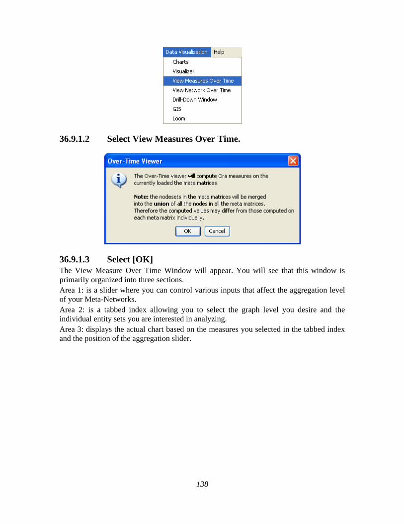
138

36.9.1.2 Select View Measures Over Time.

36.9.1.3 Select [OK] The View Measure Over Time Window will appear. You will see that this window is primarily organized into three sections. Area 1: is a slider where you can control various inputs that affect the aggregation level of your Meta-Networks. Area 2: is a tabbed index allowing you to select the graph level you desire and the individual entity sets you are interested in analyzing. Area 3: displays the actual chart based on the measures you selected in the tabbed index and the position of the aggregation slider.

139

36.10 Interpreting The Results After Performing View Measures Over-Time Analysis

In the example above, we have loaded all three of our network time captures into the View Measures Over Time Analysis tool. The result of our analysis, as we have indicated before, will be displayed as a chart in the bottom section of the ORA interface in Panel 3. But, what does this tell us? To find out, we will examine the Graph Level measure Knowledge Waste. From the tabbed measures window:

140

36.10.1.1 Graph tab > Congruence, Organization Measure, Knowledge Waste.

The result is displayed below.

We can see the chart displays an axis scale correlating to our networks over time. The graph level measure of Knowledge Waste was selected using the View Measures Over Time tool and the result is displayed in the chart area of the window. We can see that the graph level measure of Knowledge Waste held a value slightly above 40 in the first Meta-Network, 1996, displayed with 1 on the Time axis. We can deduce from the chart that in 1997 something affected our measure of Knowledge Waste to increase the value to nearly 60. This corresponds to the time scale axis of 2, which represents 1997, our second year of network data. In the final year, 1998, our measure of Knowledge Waste declined to the value in 1996. This should be visually evident with its relative line graph position. It is clear that the value for the Knowledge Waste Measure increased from the first Meta-Network (1996) to the second (1997) and then retreated back to its original (1996) level. It would be up to you to determine what may have affected that measure for it to undergo this progression and regression.


At this point, you should be able to complete the following tasks to perform a View Measures Over-Time Analysis:

141

• Load multiple data files into ORA (in the form of Meta-Networks) representative of your network across certain periods of time.

• Select an aggregation level and choose a graph level or entity set to analyze. • Analyze the data output in the charting tool located in the bottom section of the

View Measures Over Time window. • See how your network may have changed from one time capture to the next for

any given graph level or entity node measure. • Use this visual comprehension to draw conclusions about how your network

changed across multiple time period.

142

37 Lesson 8: Network Converter 37.1 Load Network

The Network Converter is used for changing dataset file formats.

If you have Analyst Notebook data then select the [Analyst Notebook >>>] button to reveal the section. Select the [<<< Analyst Notebook] button to hide it.

37.2 Transform Network

143

Create bipartite: Creates a set of nodes decomposed into two disjoint sets such that no two nodes within the same set are adjacent.

Remove isolate nodes: If the Meta-Network you are transforming contains any Isolate nodes they will be removed in the transformed Meta-Network.

Remove pendant nodes: If the Meta-Network you are transforming contains any Pendants nodes they will be removed in the transformed Meta-Network.

Symmetrize by method: The two options are Minimum or Maximum. Symmetrizing turns a directed or asymmetric network data into un-directed or symmetric data. Both methods use a pair of values from the upper and lower portions of the table

[Transform] button: Performs any of the checkmarked functions above.

144

[Make IDs Canonical] button: Removes leading and trailing spaces, replaces internal spaces with underscores, replaces apostrophes with dashes, and converts everything to lowercase. (NOTE: works on IDs only, does not touch the Title Attribute)

[Load and Apply Thesaurus] button:

Make thesaurus canonical:

[Move Node IDs to Node Titles] button: Moves the values in the Entity ID column into the Entity Title Column and renumbers the Entity ID.

[Move Titles IDs to Node IDs] button: Moves the values in the Entity Title column into the Entity ID column and deletes the Entity Title column.

145

37.3 Node Sets

The Node Sets tab allows you to alter what, and how, a Meta-Network will be converted. It starts with a list of the NodeSets and empty checkboxes

37.4 Nodes Add

You can add a node to any set by placing a checkmark in the NodeSets' box and selecting the [Add] button. For this example a checkmark was placed in the Agent box and the [Add] button is selected. The dialog box will ask how many nodes you want to add.

Type in the number of nodes to add, in this case we'll only add 1, and select [OK]. The AGENT section accordians to show a new agent node, 17.

146

37.5 Nodes Delete

Now say you want to delete an agent, say 17. Place a checkmark in the checkbox and select the [Delete] button and it will be removed.

147

37.6 Nodes Merge

The third button in the Nodes section is [Merge]. With this function you can combine two or more nodes into a single node. Here I place checkmarks next to the members of SG-1 to combine them into a single node.

148

After selected the [Merge] button the Merge AGENT Nodes dialog asks me to give it both an ID and Title. I give it an ID unique from the original dataset, A17, and an unique Title, sg-1.

col_jack_o'neill, daniel_jackson, maj-samantha_carter, & teal'c have been removed and the new node, sg-1 has been added.

149

37.7 Node Properties

This section allows you to Add/Edit/Delete attributes to individual Nodes in a NodeSet. One important plot point was finding a human who spoke Gou'ald, and that was daniel_jackson. Place a checkmark in his box.

151

Select the [Add] button to bring up the Add AGENT Attribute window. in ID: type in the name of the new attribute. In Title: type in the value. Then select [OK].

daniel_jackson now has the attribute speak-gou'ald=yes.

152

But other agents also spoke the language. But instead of adding them one at time place a checkmark in the box next to each agent that will receive that attribute. Then select [Add] and specify the attribute and value as done previously. NOTE: Be sure to spell the attribute the same or ORA will add it as a different attribute.

Save this new MetaNetwork under a new name. Select the Save Network tab, select the [Save…] button, and save it under a new name in the directory of your choice. Close the Network Converter window.

153

Open up the new MetaNetwork form the main menu, File ⇒ Open Meta -Network…. Viewing the agent NodeSet, select the Editor tab. A new attribute column, speak_gou'ald, shows the values inserted by the Network Converter.

154

37.8 Graphs

37.9 Save Networks

155

38 Basic Lesson in Automap

156

Using a Concept List

38.1 Description

Concept Lists (the frequency of concepts in one file) and Union Concept Lists (the frequency of concepts throughout all loaded files) can be used to work with concepts from one or more text files. It lists the frequency, relative frequency, and gram type. When working with multiple files you'll find the Union Concept List useful.

38.1.1.1.1.1 NOTE : The number of unique concepts considers each concept only once. The number of total concepts considers repetitions of concepts.

38.2 Concept List Procedure

38.2.1 1. Select a text file(s) to use

Place your text file(s) in an empty directory. Load the file(s) by selecting from the Pull Down Menu File => Select Input Directory.

38.2.1.1 theBoy.txt:

See the boy named Dave. He has 2 balls. 1 ball is red. 1 ball is blue.

38.2.1.2 milkAndCookies.txt:

Dave wants milk and cookies. He drives to the store. Then he buys milk and cookies.

38.2.2 2. Create Concept List

From the Pull Down Menu select Generate => Concept List. Navigate to where you want to save the file(s) and click Select.

38.2.3 3. Decide if you need Union Concept List

After specifying the directory for the Concept List(s) AutoMap will ask if you want to create a Union Concept List. Unless you know you will not need it, click Yes.

157

38.2.4 4. Review a Concept List in the Concept List Viewer

The Concept List(s) and Union Concept List can be viewed using Concept List Viewer. From the Pull Down Menu select Tools => Concept List Viewer. From the Viewer Pull Down Menu select File => Open File and navigate to the location of the concept list to view.

38.3 Concept List Viewer functions

38.3.1 Sorting a Concept List

A Concept List can be sorted by clicking on any of the headers. This will sort the list in an ascending order. Clicking the same header again will reverse the sorting order to descending. Which header is being used will be denoted by a small triangle to the left of the header name.

38.3.1.1.1.1 NOTE : The small triangle to the right of the header will tell you which header is used for sorting and whether it's in ascending upward facing arrow or descending downward facing arrow order.

38.3.2 Creating a Delete List

A Delete List can be created from the Concept List Viewer. Place a check mark in the Selected column of each concept to include in a Delete List. From the Pull Down Menu select File => Save as Delete List. AutoMap will prompt you to select a location to save the Delete List. Give it a unique filename and click Open.

158

38.3.2.1.1.1 NOTE : The Delete List can be saved in either the .txt or a .csv format.

This new Delete File can now be loaded and applied to your texts.

38.3.3 Selecting Concepts

In the Viewer Edit menu the viewer gives you options for selecting/deselecting multiple concepts.

Select All : Places a check mark in every check box.

Select None : Clears all check marks from the concept list.

Select Greater Than : Allows the user to set the frequency threshold which will select only those concepts whose frequency is That value or greater.

You can also manually select and deselect individual concepts by using the check marks in the Selected column.

38.3.4 Compare Files

AutoMap can compare a second file to the currently loaded concept list. The viewer will display concepts found in only one file in either red or green. Concepts found in both files remain on a white background.

38.3.4.1 milkAndCookies.txt

Dave wants milk and cookies. He drives to the store. Then he buys milk and cookies.

38.3.4.2 theBoy.txt

See the boy named Dave. He has 2 balls. 1 ball is red. 1 ball is blue.

From the Viewer Pull Down Menu select File => Open File and navigate to the first concept file. From the Viewer Pull Down Menu select File => Compare Files and navigate to the second concept file to compare.

159

38.3.4.2.1.1 For demonstration purpose I have done a Edit => Select All before I ran Compare files so it was possible to see which concepts belong to the first file before using File => Compare Files. This is not normal procedure.

Unhighlighted with a check mark : These concepts appear in both files.

Red highlight with a check mark : These concepts appear only in milkAndCookies.txt.

Green highlight without a check mark : These concepts appear only theBoy.txt.

The importance of this function allows you to see which concepts are unique to individual files. If also assists in determining concepts which can be considered unneeded or unwanted.

38.4 Concept List and Stop Characters

It's important to know that certain punctuation act as stop characters when generating a Concept List. When AutoMap encounters an apostrophed or hyphened name it considers the parts before and after these punctuation as separate concepts.

160

38.4.1.1.1.1 O'Neill would be seen as two concepts: O and Neill and al-jazeera would be seen as two concepts: al and jazeera.

Using a Delete List

38.5 Description

Delete Lists allow you to remove non-content bearing conjunctions, articles and other noise from texts. It also allows you to delete concepts that you just don't care about for analysis purposes.

Delete Lists can be created internally in AutoMap or externally in a text editor or spreadsheet. They are a preprocessing stage done before doing any output.

38.5.1.1.1.1 NOTE : Whether you apply the Delete List(s) before or after applying a Thesauri will depend on your exact circumstances. AutoMap allows for applying multiple Delete Lists is that is a necessity, one before and one after.

38.6 Delete List Procedure

38.6.1 1. Select a text file(s) to use

Place the text to use in an empty directory. Below is an example text.

38.6.1.1 Text:

Ted lives in the United States of America. He lives on a dairy farm. He considers it a good life. Would he ever consider leaving?

38.6.2 2. Create a Concept List

To create a Delete List it helps to know the frequency of the concepts in the files. From the Pull Down Menu select Generate => Concept List. Save the file in your output directory.

38.6.3 3. Create a Delete List

A Delete List can be created within AutoMap using the Concept List Viewer. From the Pull Down Menu select Tools => Concept List Viewer. Navigate to the directory containing the Concept List file and select a file. In the Viewer place a check mark in the

161

Selected column next to the concepts to include. From the View Pull Down Menu select File => Save as Delete List. Save the file in your support directory. The Delete List created can be viewed in the Delete List Viewer by selecting Tools => Delete List Viewer.

A Delete List can also be created in Excel. Load the Concept List in Excel and sort by the frequency column. Create a new column and label it Delete List. Place an X next to all concepts to include in the Delete List. Sort the spreadsheet by the Delete List column. Copy all the rows containing an X in the Delete List column. Create a new sheet and paste these rows into it. Delete the column with the Xs. Save this file as a .txt file.

38.6.3.1.1.1 NOTE : For large concept lists review the top 100 entries and add concepts to the Delete List items. Resort primarily by the Delete List column and secondarily by the concept column. Review the top 100 again. Repeat this process until the top 100 entries are of interest. review the rest of the list for other unneeded or unwanted concepts. Save this list as a .txt file.

38.6.3.1.1.2 TIP : Create a cut-off limit (e.g. a word needs to be used at least three times. Concepts used less than that are placed on the Delete List.

38.6.3.2 Delete List:

Below is the Delete List created for the example file.

in the of he on a it

38.6.4 4. Apply a Delete List

From the Pull Down Menu select Preprocess => Apply Delete List. Navigate to the directory where your delete list is stored.

38.6.5 5. Adjacency Option

AutoMap will ask what type of adjacency you what to use. The Adjacency option determines whether AutoMap will replace deleted concepts with a placeholder or not.

• Direct Adjacency : Removes concepts in the text that match concepts specified in the delete list and causes the remaining concepts to become adjacent.

162

• Rhetorical Adjacency : Removes concepts in the text that match concepts specified in the delete list and replaces them with (xxx). The placeholders retain the original distances of the deleted concepts. This is helpful for visual analysis.

38.6.6 6. The newly pre-processed texts can be viewed in the main window.

38.6.6.1 Delete List with Rhetorical Adjacency

Ted lives xxx xxx United States xxx America. He lives xxx xxx dairy farm. He considers xxx xxx good life. Would he ever consider leaving?

38.6.6.2 Delete List with Direct Adjacency

Ted lives United States America. He lives dairy farm. He considers good life. Would he ever consider leaving?

38.6.6.2.1.1 NOTE : If using Direct Adjacency the concepts are NOT replaced with anything. The concepts are moved next to the ones before and after. For more information on Delete Lists see the Content section.

38.6.6.2.1.2 NOTE : If you need to remove the Delete List it can be Un-applied using the Undo function under the Pull Down Menu Preprocess or from the quick launch buttons.

38.7 Other Delete List Functions

38.7.1 Multiple Delete Lists

Multiple delete lists can be applied to the same text in any order the user wants. They can be viewed in order using the Pull Down Menu.

38.7.1.1.1.1 NOTE : This is useful if you have multiple specialty Delete Lists.

38.7.2 Modifying a Delete List

After a Delete list is created you can modify it using the Delete List Editor. From the Pull Down Menu select Tools => Delete List Editor. From the View Pull Down Menu select Open File and navigate to the Delete List to view.

163

From this window you can:

• Add Concepts: In the textbox above the list type one new concept then click [Add Word]. Your new concept will be added to the list. Repeat until you've added all concepts necessary. The next time you save the Delete List it will be saved without the checked concepts.

• Remove Concepts : Click in the check box next to the concept to remove in the Select to Remove column.. The next time you save the Delete List it will be saved without the checked concepts.

38.7.2.1.1.1 NOTE : No concepts are added or deleted until you actually save the file. • Create New Delete List : From the viewer Pull Down Menu select File => Save

as Delete List. AutoMap will prompt you to select a directory and give the file a new file name.

38.7.2.1.1.2 NOTE : Make sure to give the file the .txt extension.

38.7.3 Save text(s) after Delete List

After applying a Delete you can save your texts by selecting from the Pull Down Menu File => Save Preprocess Files. This step must be done before any other preprocessing as this option saves the texts at the highest level of preprocessing.

164

Using a Generalization Thesaurus

38.8 Description

Thesauri are generally used to take multiple concepts, in different forms, and compile them under one key concept. If this is not done then the same concept could be listed many times as individual concepts.

38.9 Thesauri Procedure

38.9.1 1. Select your text file(s)

Copy these files into a text editor and save them as johnSmith.txt and countryThesauri.csv. Place the johnSmith.txt in a folder by itself. Place countryThesauri.csv in an accessible folder other than where johnSmith.txt resides.

38.9.1.1 johnSmith.txt

John Smith lives in the USA. He is a United States citizen.

38.9.2 2. Prepare your Thesauri

For this simple file the thesauri is short. Larger texts could easily have hundreds of entries. This can be done in either a text editor or a spreadsheet.

165

38.9.2.1.1.1 NOTE : It's important to put your thesaurus in a string length order to get a meaningful result. If not your results might not be programatically correct. More importantly this will not result in an error message.

38.9.2.2 thesauri.csv The United States of America,United_States United states,United_States John Smith,John_Smith America,United_States U.S.,United_States

38.9.3 3. Loading the files

From the main menu select File => Select Input Directory. Navigate to the directory where you placed johnSmith.txt and click Select. The file will appear in the main window.

38.9.4 4. Applying the thesauri

From the main menu select Preprocess => Apply Generalization Thesauri. Navigate to the directory where you placed countryThesauri.csv and click Select. The thesauri will be applied and a new text will appear in the window with the thesauri substitutions. Apply Thesauri (2) will now appear in the dropdown menu denoting AutoMap has applied the thesauri.

38.9.4.1 johnSmith.txt after thesauri applied

John_Smith lives in the United_States. He is a United_States citizen.

38.10 Thesauri Editor

AutoMap contains a Thesauri Editor making it easy to revise your thesauri files. From the dropdown menu select Tools => Thesauri Editor.

From the Thesauri Editor menu select File => Open File. Navigate to the directory with your thesauri and click [Okay]. From the Thesauri Editor you can make changes to the thesauri.

38.11 Questions regarding Thesauri

38.11.1 Different Thesauri for different purposes

You might initially think it's necessary to keep all the thesauri entries in one place. Just easier to find everything. But it essence it would make it easier to keep track by splitting

166

up the thesauri into smaller files, each with it's own purpose. Below are some of the specialty thesauri used in this lesson.

You might have a general countries thesauri that is always used to fix multiple ways of posting a country. The U.S. can be listed in a multitude of ways:

U.S., America, United States, The United States of America

A country thesauri could have all these permutations listed and convert them all to the same concept say, United_States. So instead of four individual concepts you would have one.

U.S.,United_States America,United_States United states,United_States The United States of America,United_States

If your project concentrates on a particular field you could have a thesauri that contains names of organizations, resources, or people's names which appear with regularity.

Analysts working on a similar subject every day would need the same names, places, and resource for each run. A special thesauri could take care of that and would be easier to maintain as a single file.

38.11.2 Running the Delete List Before or After the Thesauri

You may also find it necessary to run a Delete List on your files. Whether you apply a delete list before or after applying a generalization thesauri will depend on your set of files. A longer discussion can be found in the Content section under Process Sequencing.

38.11.3 Using of one large thesauri vs. multiple smaller thesauri

This will be a personal choice of the user. Multiple thesauri have the advantage of easier editing but the downside is needing to apply multiple thesauri to the same set of files.

167

38.11.3.1.1.1 NOTE : When doing multiple runs on the same data some analysts prefer to maintain a single thesaurus.

First Run with the GUI

38.12 Description

This is an overview of your first run of AutoMap3. It is not an all-inclusive view of AutoMap but will cover the, more or less, necessary basics.

38.13 Procedure

38.13.1 1. Create Workspace

A good starting point is creating a project directory, a place where all your input files and output files will reside. This helps prevent files from getting lost. One suggestion is to create a top level project directory and create input and output directories within that directory. I also create a directory to place all support files such as Delete Lists and all the Thesauri.

Place all your input files into the input directory. Place any Delete Lists, Thesauri and other files to be used in the support directory. Direct all your results to the output directory.

168

38.13.2 2. Preparing Your Files

Files can come from any source. But to use in AutoMap3 they must be .txt files. Files in a Word format or html files will not be accepted into AutoMap. Any of these formats must be re-saved as a .txt format. This could be as simple as re-saving the file in the correct format to doing a copy-and-paste of the text into a text editor.

38.13.2.1.1.1 NOTE : AutoMap accepts a variety of text encodings but they must be in a .txt format.

38.13.3 3. Load your files into AutoMap

Once the text files are in the correct format they can be loaded into AutoMap. From the Pull Down Menu select File = Select Input Directory and navigate to the directory where you placed your text files. The first of these files will appear in the main window.

38.13.3.1 johnSmith.txt

John Smith lives in the USA. He is a United States citizen.

169

38.13.4 4. Decide on the Preprocessing Functions to use

Functions from the Preprocessing Menu affect all loaded text. None of these functions create any output files (though some require externally created files to work). These functions remove excess concepts (e.g. Remove Punctuation, Numbers, extra white spaces, or Symbols) or modify concept names (e.g. Thesauri for creating key_concepts) for easier generation and post-processing functions.

38.13.5 5. Creating a Generalization Thesaurus

Many people, places and things can be known by a variety of different formats of their names. A General Thesauri helps consolidate these various names under one unifying term. Below is an example. The format is concept,key_concept. Concept can be one or more words but key_concept must be one single word which can use the underscore.

170

John Smith,John_Smith United States,United_States_of_America USA,United_States_of_America

38.13.5.1.1.1 NOTE : The Thesaurus changes both the 2nd and 3rd concepts to the key_concept United_States_of_America.

Create this file in a text editor or spreadsheet program and save it as a .csv file.

38.13.6 6. Apply a Generalization Thesaurus

From the Pull Down Menu select Preprocess => Apply Generalization Thesauri and navigate to your Generalization Thesaurus. After applying the text will change to reflect the application of the thesaurus.

38.13.6.1 johnSmith.txt after General Thesauri applied

John_Smith lives xxx xxx United_States_of_America. He xxx xxx United_States_of_America citizen.

38.13.7 7. Edit your General Thesauri

After applying a Thesaurus the list can be altered by selecting from the Pull Down Menu Tools => Thesauri Editor.

38.13.8 8. Delete Extra/Unneeded Concepts

Texts usually have many extra concepts, or noise, that are not relevant to the semantic connections. A Delete List removes those extra words. From the Pull Down Menu select Preprocess => Apply Delete List and navigate to the Delete List you want to use. The text in the main will change to reflect the application of the Delete List.

38.13.8.1 Delete List

Delete List for example text.

in the is a

38.13.8.2 johnSmith.txt after Delete List with rhetorical adjacency

John Smith lives xxx xxx USA. He xxx xxx United States citizen.

171

38.13.9 9. View and Alter Delete Lists

After creating Delete List you may want to make changes to it with the Delete List Editor. From the Pull Down Menu select Tools => Delete List Editor. From this tool you can add or remove concepts from a Delete List. From the Pull Down Menu select File => Save as Delete List and either replace the old file or save it as a new file.

38.13.9.1.1.1 NOTE : If you decide to make changes to the Delete List then Undo the applied Delete List and reapply the new one.

38.13.10 10. Generate Output

After preprocessing the text it's time to produce output from them. The Pull Down Menu Generate contains functions that tell AutoMap to write output for the function selected; Concept Lists, Semantic List, Parts of Speech, and other useful functions.

Each function outputs files that can be examined for analysis and used to further process the text files.

38.13.11 11. Example of Output for Concept List

From the Pull Down Menu select Generate => Concept List. AutoMap will ask for the directory to save the concept list.

172

concept,frequency,relative_frequency,gram_type He,1,0.33333334,single John_Smith,1,0.33333334,single United_States_of_America,2,0.6666667,single citizen,1,0.33333334,single lives,1,0.33333334,single xxx,4,1.3333334,single

Extracting a Semantic Network

38.14 Description

Text files have connections but they are some times difficult to see. You can load your text files into AutoMap and process them to create semantic networks which are viewable in ORA.

This lesson details processing text files in AutoMap to extract a Semantic Network, how to view it in ORA, and which reports are used in analysing semantic networks.

38.14.1 What is a Semantic Network?

Semantic networks are knowledge representation schemes involving nodes and links between nodes. It is a way of representing relationships between concepts. The nodes represent concepts and the links represent relations between nodes. The links are directed and labeled; thus, a semantic network is a directed graph.

38.15 Procedure

Throughout this lesson we will be using the following two files below: dairyFarm.txt and breadAndMilk.txt. You can copy this text in a text editor and create your own files. Place them in your designated input directory.

38.15.1.1 dairyFarm.txt

John Smith runs a dairy farm in the USA. John's farm has Jersey cows. His milk gets the USDA seal.

173

38.15.1.2 breadAndMilk.txt

John and Mary Smith need milk and bread. They drive to the Mega Mart supermarket. Mary buys milk and bread and John buys cookies.

38.15.2 Load text documents into AutoMap

Place all the text files for conversion into a single folder. From the Pull Down Menu select File => Select Input Directory. The first text will be displayed in the main window and the filename will appear in the Filename Box. Using the File Navigation Buttons you can navigate through the loaded files.

38.15.3 Build a General Thesauri

Many people, places and things are made of two or more words. For example John Smith, the White House, cell phone. Before producing any output it's necessary to combine these multi-word concepts into key concepts.

38.15.3.1.1.1 NOTE : Many concepts include the definite article in their name and should be included in the thesaurus.

If you have no previous thesaurus then one will need to be created from scratch. This will require going through the text files and finding those multi-word concepts and creating a list of key concepts. The format for this is multi word concept,key_concept.

38.15.3.1.1.2 NOTE : Be sure NOT to leave any spaces before or after the comma.

38.15.3.2 Thesaurus for the files loaded Mega Mart supermarket,Mega_Mart_supermarket Jersey cows,Jersey_cows dairy farm,dairy_farm John Smith,John_Smith Mary Smith,Mary_Smith the USDA,The_United_States_Department_of_Agriculture farm,dairy_farm John,John_Smith Mary,Mary_Smith USA,United_States_of_America

38.15.4 Apply a General Thesauri

After the thesaurus is created it is time to apply it to the text. From the Pull Down Menu select Preprocess => Apply Generalization Thesauri. Navigate to the directory where the thesauri is saved and click [Select].

174


John_Smith runs a dairy_farm in the United_States_of_America. John_Smith 's dairy_farm has jersey_cows. His milk gets The_United_States_Department_of_Agriculture seal.

38.15.4.2 breadAndCookies.txt

John_Smith and Mary_Smith need milk and bread. They drive to the Mega_Mart_supermarket. Mary_Smith buys milk and bread and John_Smith buys cookies.

Notes about Thesaurus Building: 1. In this example John and Mary were converted to John_Smith and

Mary_Smith as there are a small number of agents. In larger texts you will not be able to make an assumption like that as there may be multiple agents with the same first name.

2. The definite article in the concept the USDA was placed in the Thesaurus instead of being deleted in the Delete List.

38.15.5 Remove Punctuation

In dairyFarm.txt there is a possessive, John Smith's. After the thesaurus is applied it becomes John_Smith 's. Removing punctuation will delete the apostrophe.

From the Pull Down Menu select Preprocess => Remove Punctuation. In this example the apostrophe is the only item removed.


John_Smith runs a dairy_farm in the United_States_of_America. John_Smith s dairy_farm has jersey_cows. His milk gets The_United_States_Department_of_Agriculture seal.


John_Smith and Mary_Smith need milk and bread. They drive to the Mega_Mart_supermarket. Mary_Smith buys milk and bread and John_Smith buys cookies.

175

38.15.6 Create the Concept Lists

Now you need to create a Delete List to remove unneeded and unwanted concepts. This is done by first creating a Concept List. This will assist us in determining unneeded and unwanted concepts.

From the main menu select Generate => Concept List. Navigate to the directory to save the files and click [Select]. AutoMap will ask if you want to create a Union Concept List. Click [Yes] as you will need this fill later.

A Concept List will be created for each file. But the file you're interested in is The Union Concept File which contains entries for all text files loaded.

38.15.6.1.1.1 TIP : It's advisable to create individual directories for your results to assure that AutoMap doesn't overwrite these files in a future run.

38.15.7 The Delete List

A Delete List will now be used to remove unneeded and unwanted concepts. These consist of articles, preposition, and other concepts which you know will not be of any value in an analysis.

38.15.8 Build a Delete List in Excel

Open up Excel and load the Union Concept file. If you do not see the file in the directory make sure Excel can see All Files (*.*).

Insert a column to the right of the concept column. Select the entire worksheet. Sort the sheet on the frequency column from Largest to Smallest. Place an X in the newly inserted column for the terms you want in your Delete List. Select the entire worksheet again and sort on the column, Z to A where you placed the Xs. These concepts are you Delete List.

Highlight and copy those values, create a new worksheet, and paste them into a new worksheet. Save this worksheet as a .csv file.

176

38.15.9 Build a Delete List in AutoMap

AutoMap also contains a tool for creating a Delete List, the Concept List Viewer. From the Pull Down Menu select Tools => Concept List Viewer. From the viewer menu select File => Open File. Navigate to the directory containing the newly created Union Concept List and click [OK].

To build a Delete List place a check mark in the Selected column for all the concepts you wish to delete. The list in use here contains: **put the list of words here**. From the viewer menu select File => Save Delete List and navigate to where you want to save the Delete List file. Close the Viewer.

177

38.15.10 Apply a Delete List

From the main menu select Preprocess => Apply Delete List. Navigate to the directory with your newly created file and click [OK]. You will be asked whether you want Rhetorical (replaces deleted concepts with a placeholder xxx) or Direct (removes the concept entirely) adjacency. I choose rhetorical in this instance. Below is the results for the two files.


John_Smith xxx xxx dairy_farm xxx xxx United_States_of_America. John_Smith xxx dairy_farm xxx jersey_cows. xxx milk xxx The_United_States_Department_of_Agriculture seal.


John_Smith xxx Mary_Smith xxx milk xxx bread. xxx xxx xxx xxx Mega_Mart_supermarket. Mary xxx milk xxx bread xxx John_Smith xxx cookies.

178

38.15.10.2.1.1 NOTE : The placeholder xxx will not output to the DyNetML file as a concept.

38.15.11 Create a DyNetML file

It's now time to generate the DyNetML. From the Pull Down Menu select Generate => Semantic Network. AutoMap will output one XML file for each text file loaded. AutoMap will ask a couple of questions as to how you want to format the DyNetML file.

• Directionality : Choose either Unidirectional or Bidirectional. Unidirectional will consider only words that come after it. Bidirectional will consider words both after and before it. (This example uses Unidirectional)

• Select Window Size : Determines the distance a concept can be to another and be connected. (This example uses 5)

• Select Stop Unit : Options are Clause, word, sentence paragraph, or all. (This example uses sentence)

• Select Number of Sentences : (This example uses 1)

38.16 Loading files into ORA

Start ORA. From the menu select File => Open MetaNetwork. Navigate to the directory with the files created in Automap. Select a file(s) and press [OK]. Selecting multiple files can be done by holding down the [CTRL] key while clicking on each file..

38.16.1.1.1.1 NOTE : If there are already file(s) loaded into ORA, choose the Append As Additional Meta-Network option.

38.16.2 Visualize your meta-networks

In the left panel of ORA highlight one of the newly loaded Meta-Network. Then press the Visualize this Meta-Network. That file will appear in the Visualizer.

179

38.16.2.1.1.1 NOTE : The concept xxx remains in the dataset. This will be removed in the Visualizaer.

Once the file is loaded into the Visualizer click the Show Arrows button on the Visualizer menubar to display the direction the words are going. Now right-click on the xxx node and select Hide Node.

38.17 Display the Files

The files are now displayed in ORA showing their semantic connections.

180



38.18 ORA Reports

181

There are five reports of special interest in analyzing semantic networks: Communicative Power, Hot Topics, Key Entity, Parts of Speech, and Semantic Networks.

38.18.1 Procedure

All reports are accessed from ORAs Pull Down menu Analysis -> Generate Reports. Select A Report and place a check mark next to the file(s) to analyze then press the [Next] button. Then select the formats for the reports: Text, HTML, and CSV . Navigate to the directory to save the files then enter a prefix for the files. Then press the [Finish] button.

38.18.2 Communicative Power

Concepts are classified according to whether they have high and low values for the measures: total degree centrality, betweenness centrality, and consensus. The classifications are:

Type Degree Betweenness Consensus

Ordinary low degree low betweenness low consensus

Factoids low degree low betweenness high consensus

Buzzwords low degree high betweenness low consensus

Emblems low degree high betweenness high consensus

Allusions high degree low betweenness low consensus

Stereotypes high degree low betweenness high consensus

Placeholders high degree high betweenness low consensus

Symbols high degree high betweenness high consensus

38.18.3 Hot Topics

Displays statistics on the concepts and links in the map and the distribution of concept frequencies. It lists the most frequent and the least frequent concepts in the map. It also gives information on the distribution of frequency values.

Information from this report includes: General Statistics on Total and Unique Nodes analyzed, most frequent concepts, least frequent concepts, and distribution frequencies.

182

38.18.4 Key Entity

An important report in ORA for determining Content Analysis is Key Entity. This report detects highly ranked concepts based on two measures: Dominant Knowledge (Total Degree Centrality) and Supply Chain Criticality (Betweenness Centrality).

When multiple text files are loaded into AutoMap the report is altered to reflect this. Values for the concepts are listed for both files and a %Difference column appears on the right side of the table.

• The Knowledge chart shows the concept that repeatedly ranks in the top three measures.

• Dominant Knowledge (total degree centrality) is the normalized sum of its row and column degrees.

• Supply Chain Criticality (betweenness centrality) The Betweenness Centrality of node v in a network is defined as: across all node pairs that have a shortest path containing v, the percentage that pass through v.

38.18.5 Parts of Speech

An important report in ORA for determining Content Analysis is Parts of Speech which detects and analyzes the concepts in each text. This report counts the number of times each part of speech is used in a text, or set of texts, along with other information such as the intersection and union of concepts in multiple texts.

Analyzing a single text AutoMap will determine frequency and part of speech distribution. Other tables created are Most frequent parts of speech, Total degree of centrality for parts of speech, Betweenness centrality for parts of speech, and links between parts of speech.

When analyzing two texts ORA will display one column for each text containing a count for each row plus a column showing the Percentage Difference between the two files.

When analyzing three or more texts ORA will instead display a column for the mean and the Standard Deviation plus columns for the Min and Max.

38.18.6 Semantic Networks

The Semantic Network Report gives information on each concepts in relation to the following measures: Total Degree Centrality, Betweenness Centrality, and Consensus. Each is rated as either high or low.

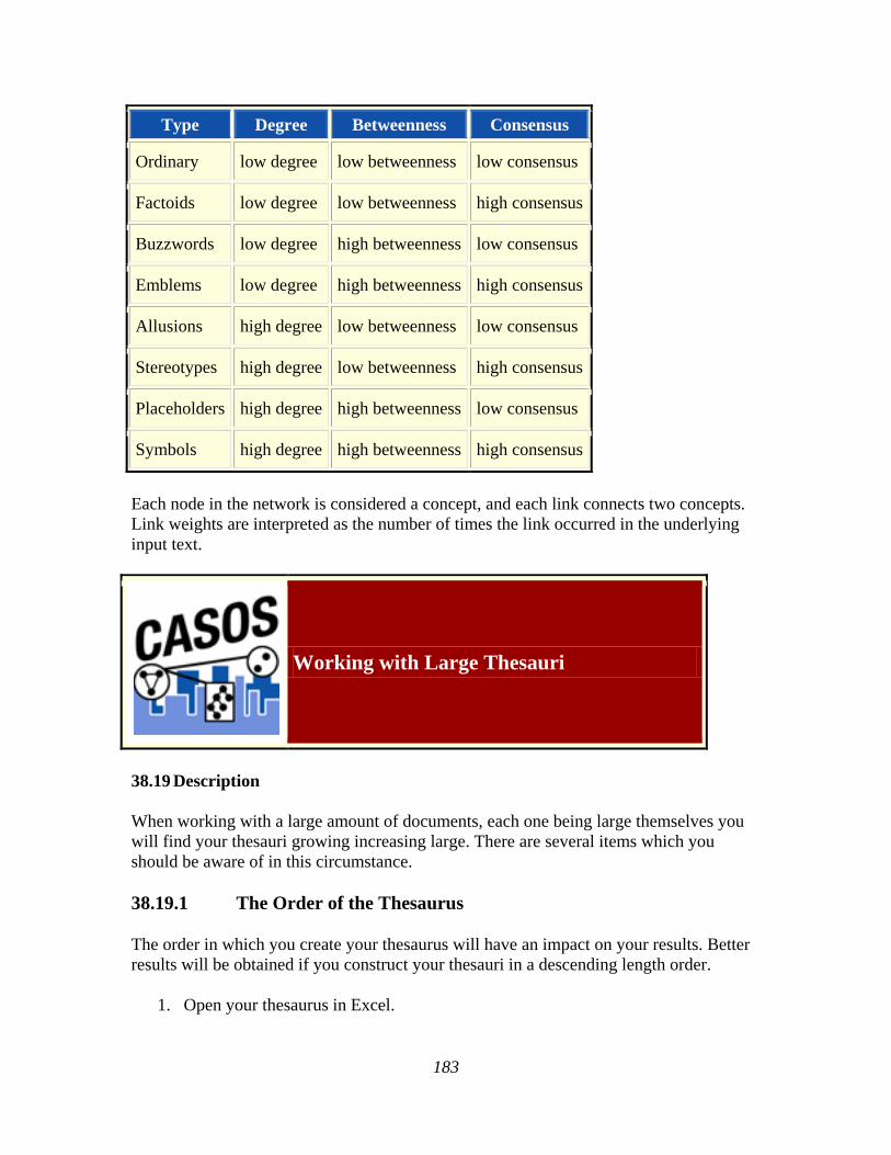
183

Type Degree Betweenness Consensus

Ordinary low degree low betweenness low consensus

Factoids low degree low betweenness high consensus

Buzzwords low degree high betweenness low consensus

Emblems low degree high betweenness high consensus

Allusions high degree low betweenness low consensus

Stereotypes high degree low betweenness high consensus

Placeholders high degree high betweenness low consensus

Symbols high degree high betweenness high consensus

Each node in the network is considered a concept, and each link connects two concepts. Link weights are interpreted as the number of times the link occurred in the underlying input text.

Working with Large Thesauri

38.19 Description

When working with a large amount of documents, each one being large themselves you will find your thesauri growing increasing large. There are several items which you should be aware of in this circumstance.

38.19.1 The Order of the Thesaurus

The order in which you create your thesaurus will have an impact on your results. Better results will be obtained if you construct your thesauri in a descending length order.

1. Open your thesaurus in Excel.

184

2. Create a new column.

3. Place the formula =len(A1). Replace the A1 with the column containing your first concept.

4. Copy and Paste Special this formula into all cells next to a concept. In the Paste Special dialog use the value option.

5. Sort the spreadsheet by the new column.

6. Delete the new column which will leave only the generalized and primary name columns.

38.19.2 Conflicts in Data

A problem can occur when you have more than one agent or location with the same name. In the beginning the text may specifically refer to John Smith and John Doe but afterwards you might find that a person is only referred to as John. AutoMap will use the first occurrence of John it finds when making substitutions.

AutoMap processes a thesaurus from top to bottom. This is why it's important to sort a thesaurus by the length of the entries.

38.19.3 Sequence of Operations

Mohammed abd al-Sha'bai

This name contains both punctuation and symbols. Depending on the order of the preprocessing you could end up with any of the following three:

Mohammed_abd_al_Sha_bai Mohammed_abd_al-Sha'bai Mohammed_abd_alShabai

38.19.4 How General Is Too General?

If you start with a 2,000 page text set, you will probably be unable to read all of the text prior to starting the processing. One of the problems you may encounter in such situations relates to common names and terms. For example, a preliminary review of the text may reveal that the documents contain an individual named Joe. Given that this is very common name, the data may contain several other individuals named Joe. Should this occur the program will incorrectly process all Joes as if they were the first Joe. Users need to exhibit caution before including common names and common terms in their thesauri.

185

If your text contains two names, Joe Smith and Joe Jones and a thesaurus entry for the name Joe then AutoMap will substitute all Joes for the first entry in the thesaurus.

38.19.5 Using the ThesauriContentOnly option

You create a MetaNetwork with the one-grams dog, cow, and farm. If you are going to use the UseThesauriContentOnly option then those three terms need to be in your General Thesaurus also. If they are not in the thesaurus then they will be eliminated from the output and the MetaNetwork will not see them to tag them.

38.19.6 Positive or Negative Links

AutoMap creates links between nodes. But AutoMap does not differentiate between positive and negative links. After processing that is up to the analyst.

The U.S. lacks formal diplomatic relations with North Korea, Bhutan, and Cuba, but has close relationships with Canada and the U.K.

Using a large window will create a fully connected graph with all links the same type. It will also make connections for all the countries involved. The reality is that there should be positive links to Canada and the U.K. and negative links to North Korea, Bhutan, and Cuba.

Using a small window size would create a link set that is wrong:

US => North Korea => Bhutan => Cuba => Canada => UK

38.19.6.1 right:

negative links: US => North Korea; US => Bhutan; US => Cuba

positive links: US => Canada; US => UK

186

First Run with the Script

38.20 Description

All of AutoMap's functions can be accessed through the script. The two required files are the AM3Script (The AutoMap program) and a .config file (designed by the user). Additional files could include Delete Lists, Thesauri, or other list files necessary by the program.

38.20.1 Create a Workspace

A good starting point is creating a project directory, a place where all your input (your text files), output (files AutoMap writes), and support (required files by certain functions) files will reside. This helps prevent files from getting lost. One suggestion is to create a top level project directory then create input, output, and support directories within that directory.

C:\My Documents\dave\project\input C:\My Documents\dave\project\output C:\My Documents\dave\project\support

38.20.2 The .config file

Find the blank .config file in the AutoMap directory and make a copy. Rename this to something regarding your project. Open it in your text editor to begin editing the file. The blank .config file will appear as below.

<?xml version="1.0" encoding="UTF-8"?> <Script> <Settings>

AutoMap textDirectory="" tempWorkspace="" textEncoding=""/>

187

</Settings> <Utilities> <PreProcessing> </PreProcessing> <Processing> </Processing> <PostProcessing> </PostProcessing> </Utilities> </Script>

38.20.3 Initial Setup

The first thing to do is tell AutoMap where your input files are and where you want the output files to be written.

<Settings> AutoMap textDirectory="C:\My Documents\dave\project\input" tempWorkspace="C:\My Documents\dave\project\output" textEncoding="" />

</Settings>

38.21 PreProcessing Functions

Now decide which functions of AutoMap you need to run on your files. These are divided into three areas: Preprocessing, Processing, and PostProcessing. Review the documentation on the various functions to decide which functions you need to run on your text.

38.21.1 A Generalization Thesaurus

Usually a Generalization Thesaurus is the first file to create. This can be done in either a text editor or spreadsheet. Create a list of single/multi word concepts from the text and the key concepts they should be translated to.

In a text editor create each pair on a single line separated by a comma. Make sure to NOT leave a space between the comma and the two items.

United States of America,United_States_of_America

188

Save this file as a .csv file.

In a spreadsheet program place the single/multi word concept in the first column and the key concept in the second column.

A B

United States of America United_States_of_America


In your project .config file in the Preprocessing section insert the command for applying a Generalization Thesaurus. Place the pathway to the newly created thesaurus in the thesauriLocation parameter and choose whether to use the thesauriContentOnly option.

38.21.1.1.1.1 NOTE : thesauriContentOnly is set to y (put only concepts from the thesaurus in the output file) or n (use all concepts form the text files).

<PreProcessing> <Generalization thesauriLocation="C:\My Documents\dave\project\support\thesauri.csv" useThesauriContentOnly="y" />

</PreProcessing>

Save the file.

38.21.2 A Delete List

After all the key concepts have been identified it's time to find the unneeded and unwanted concepts. A Delete List removes these concepts and reduces the overall number of concepts to analyze. The procedure for applying a Delete List is similar to applying a thesaurus.

In a text editor create a list of concepts to be removed from the text. Each line should contain only one concept which consists of a single word. There should be no extra spaces or punctuation included.

and the but


In a spreadsheet program place each concept to delete in a single cell in the first column

189

A

and

the

but


In your project .config file in the Preprocessing section insert the command for applying a Delete List. Put the pathway to the newly created Delete List in the deleteListLocation parameter and choose whether to use the saveTexts option.

<PreProcessing> <Generalization thesauriLocation="C:\My Documents\dave\project\support\thesauri.csv" useThesauriContentOnly="y" /> <DeleteList adjacency="r" deleteListLocation="C:\My Documents\dave\project\support\deleteList.txt" saveTexts="y"/>

</PreProcessing>

Save the file.

38.21.3 Other Preprocessing Functions

Any number of the preprocessing functions can be included in the script file in whatever order you need them. Insert the commands within the <Preprocessing tags in the order you need them performed.

38.21.3.1.1.1 NOTE : am3script will perform these function in the order they are placed in the script. Make sure you know what order you need to perform each task.

38.22 Processing Functions

Next thing to consider are the steps to take after the preprocessing is finished. These include most of the functions that output files and are based on the text after preprocessing. To run a Processing function the command is placed between the <Processing> tags.

38.22.1 Processing functions with no parameters

Processing functions which take no parameters include Anaphora, ConceptList, UnionConceptList, and NGramExtraction. Placing these tags between the <Processing> tags automatically performs these functions in the order that order.

190

<Processing> <ConceptList /> <UnionConceptList />

</Processing>

38.22.2 Processing functions with parameters

All other Processing functions require parameters to set for successful completion. This is either the location of a support file or parameters necessary to complete the function. The parameters follow the tag and are separated by a space and the value is enclosed in quotes.

<Processing> <SemanticNetworkList directional="U" resetNumber="1" textUnit="S" windowsize="5" />

</Processing>

If a tag requires a file to work then the pathway needs to be placed in the location parameter. An incorrect pathway will cause the AutoMap function to fail.

<Processing> <MetaNetwork thesauriLocation="C:\My Documents\dave\project\support\thesauri.csv" />

</Processing>

38.23 PostProcessing Functions

The last step is to determine which, if any, postprocessing functions are needed. These are used to alter the DyNetML before running in ORA. They include addAttribute, addAttribute3Col, and UnionDynetml. The addAttribute and addAttribute3Col both take an external file with a list of attributes to add. The UnionDynetml requires the unionType to create either a s semantic or m metaNetwork output file.

<PostProcessing> <addAttribute attributeFile="C:\My Documents\dave\project\support\attribute.csv" /> <unionDynetml unionType="s" />

</PostProcessing>

Output files will be written to the designated output directory.

38.24 Running the Script

After all the Preprocessing and Processing tags are completed the script can now be run.

191

Open a Command Window from the Start menu and navigate to the directory containing AM3Script. Move your .config file to this directory. At the command prompt type am3script project.config. Am3script will execute using the .config specified. Output files will be found in the directory specified in the tempWorkspace parameter.

<Settings> AutoMap textDirectory="" tempWorkspace="" textEncoding=""/>

192

</Settings>

38.24.1.1.1.1 NOTE : Be sure to leave a space between am3script and the name of your config file.

Institute for Software Research School of Computer Science Carnegie Mellon University

Pittsburgh, PA 15213

Basic Lessons in *ORA and Automap 2009casos.cs.cmu.edu/publications/papers/CMU-ISR-09-117.pdf ·...

Documents

Transcript of Basic Lessons in *ORA and Automap 2009casos.cs.cmu.edu/publications/papers/CMU-ISR-09-117.pdf ·...