Basic Electrostatics - German Research School for ... Basic electrostatics • Classical...

From Molecular to Con/nuum Physics I WS 11/12Emiliano Ippoli/| October, 2011

Basic Electrostatics

Wednesday, October 12, 2011

Emiliano Ippoliti

Review

2

Physics • Basic thermodynamics • Temperature, ideal gas, kinetic gas theory, laws of thermodynamics • Statistical thermodynamics • Canonical ensemble, Boltzmann statistics, partition functions, internal and free energy, entropy • Basic electrostatics • Classical mechanics • Newtonian, Lagrangian, Hamiltonian mechanics • Quantum mechanics • Wave mechanics • Wave function and Born probability interpretation • Schrödinger equation • Simple systems for which there is an analytical solution • Free particle • Particle in a box, particle on a ring • Rigid rotator • Harmonic oscillator • Basics • Uncertainty relation • Operators and expectation values • Angular momentum • Hydrogen atom • Energy values, atomic orbitals • Electron spin • Quantum mechanics of several particles (Pauli principle) • Many electron atoms • Periodic system: structural principle • Molecules • Two-atomic molecules (H2+,H2, X2) • Many-atomic molecules

Chemistry...

Informatics...

Mathematics...


Emiliano Ippoliti

Coulomb’s law

3

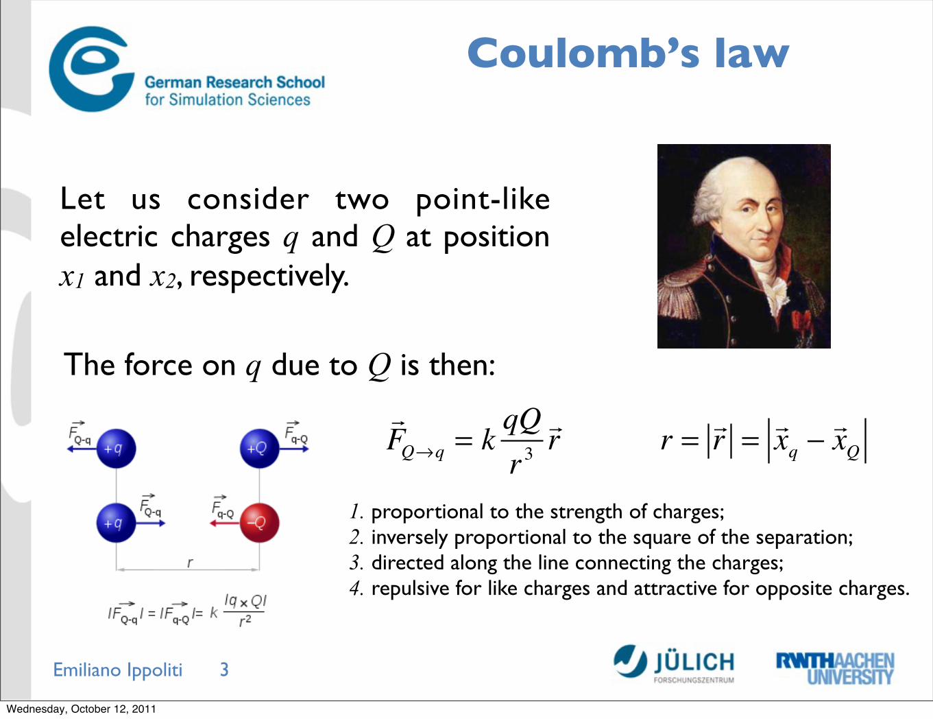
Let us consider two point-like electric charges q and Q at position x1 and x2, respectively.

The force on q due to Q is then:

FQ→q = k

qQr3r r = r = xq −

xQ

1. proportional to the strength of charges;2. inversely proportional to the square of the separation;3. directed along the line connecting the charges;4. repulsive for like charges and attractive for opposite charges.


Emiliano Ippoliti

Units

4

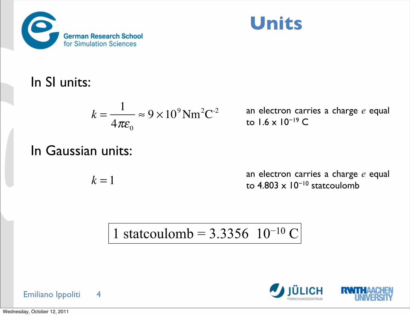
In SI units:

In Gaussian units:

k = 14πε0

≈ 9 ×109Nm2C-2

k = 1

an electron carries a charge e equal to 1.6 x 10−19 C

an electron carries a charge e equal to 4.803 x 10−10 statcoulomb

1 statcoulomb = 3.3356 10−10 C


Emiliano Ippoliti

Electric field

5

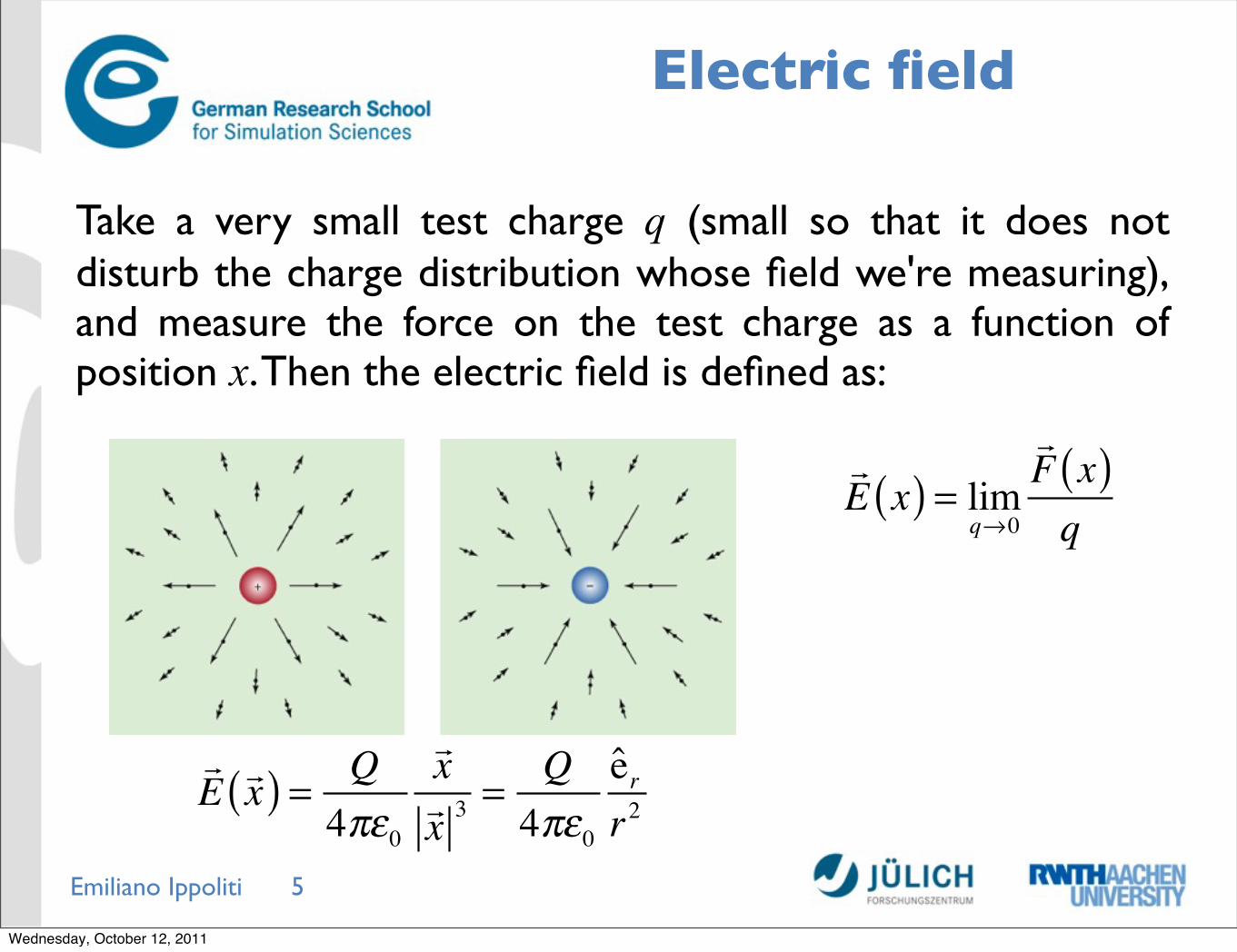
Take a very small test charge q (small so that it does not disturb the charge distribution whose field we're measuring), and measure the force on the test charge as a function of position x. Then the electric field is defined as:

E x( ) = lim

q→0

F x( )q

E x( ) = Q

4πε0

xx 3 =

Q4πε0

err2


Emiliano Ippoliti

Superposition principle

6

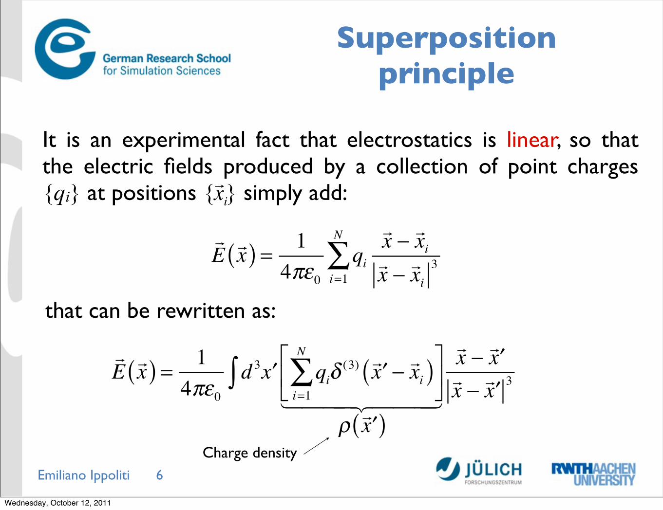
E x( ) = 1

4πε0qi

i=1

N

∑x − xix − xi

3

It is an experimental fact that electrostatics is linear, so that the electric fields produced by a collection of point charges {qi} at positions { } simply add:

xi

that can be rewritten as:

E x( ) = 1

4πε0d 3 ′x qi

i=1

N

∑ δ (3) ′x − xi( )⎡⎣⎢

⎤⎦⎥

ρ ′x( )

x − ′xx − ′x 3∫

Charge density


Emiliano Ippoliti

Dirac delta function

7

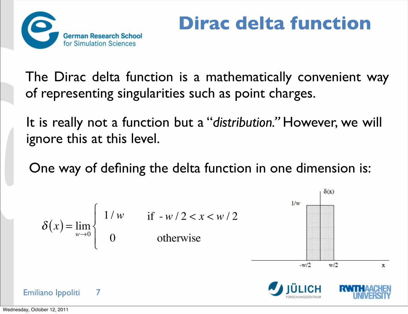
The Dirac delta function is a mathematically convenient way of representing singularities such as point charges.

It is really not a function but a “distribution.” However, we will ignore this at this level.

One way of defining the delta function in one dimension is:

δ x( ) = limw→0

1 / w if -w / 2 < x < w / 2

0 otherwise

⎧⎨⎪

⎩⎪


Emiliano Ippoliti

Dirac delta function Properties

8

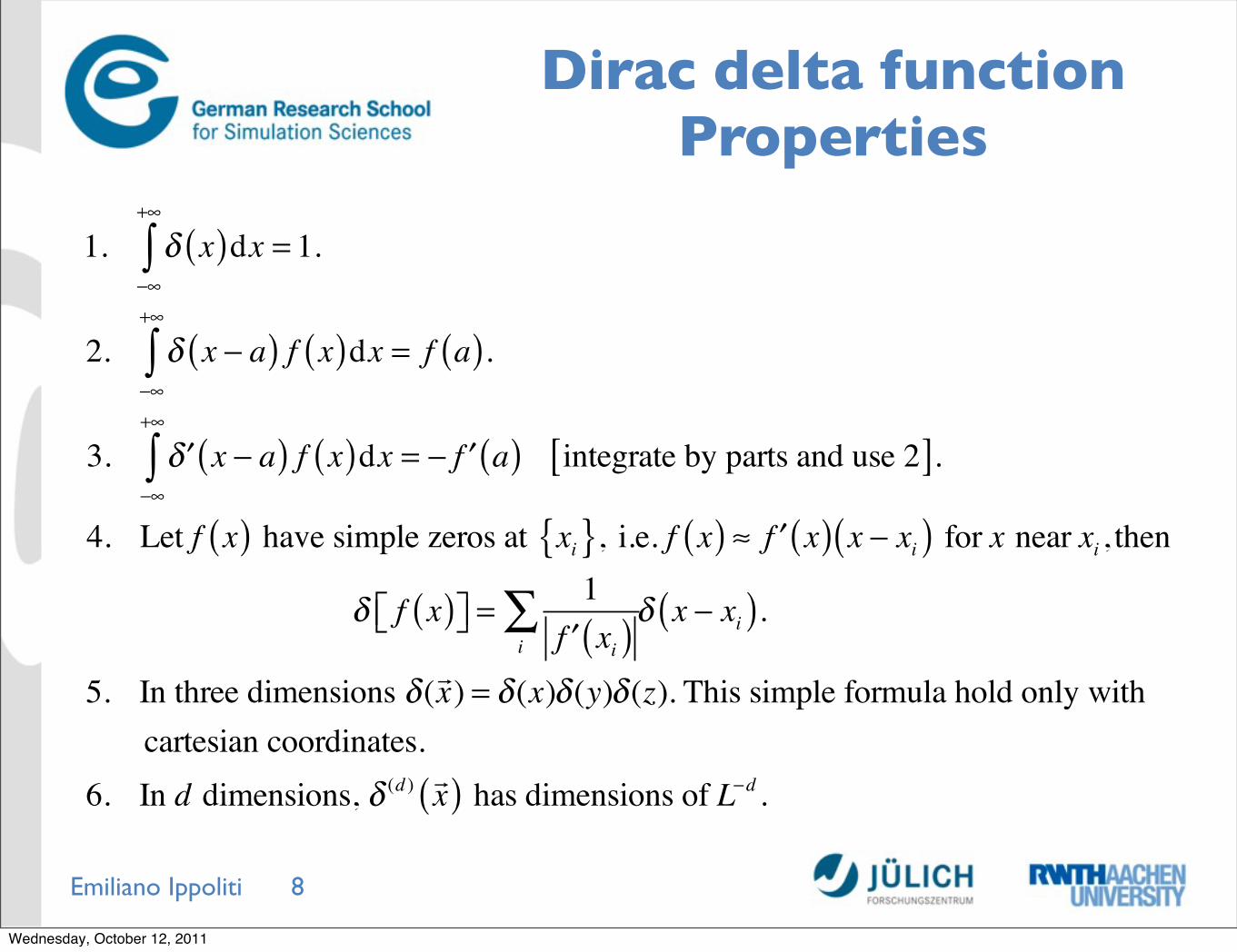
1. δ x( )dx−∞

+∞

∫ = 1.

2. δ x − a( ) f x( )dx−∞

+∞

∫ = f a( ).

3. ′δ x − a( ) f x( )dx−∞

+∞

∫ = − ′f a( ) integrate by parts and use 2[ ].

4. Let f x( ) have simple zeros at xi{ }, i.e. f x( ) ≈ ′f x( ) x − xi( ) for x near xi , then

δ f x( )⎡⎣ ⎤⎦ =1′f xi( )i

∑ δ x − xi( ).

5. In three dimensions δ (x) = δ (x)δ (y)δ (z). This simple formula hold only with cartesian coordinates.

6. In d dimensions, δ (d ) x( ) has dimensions of L−d .


Emiliano Ippoliti

Gauss’ law

9

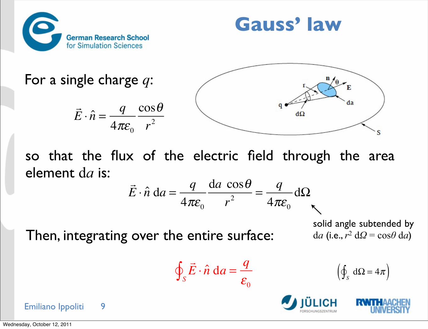
For a single charge q:

E ⋅ n = q

4πε0cosθr2

so that the flux of the electric field through the area element da is:

E ⋅ n da = q

4πε0da cosθ

r2=

q4πε0

dΩ

solid angle subtended by da (i.e., r2 dΩ = cosθ da)Then, integrating over the entire surface:

E ⋅ n da

S∫ =qε0

dΩS∫ = 4π( )


Emiliano Ippoliti

Differential form of the Gauss’ law

10

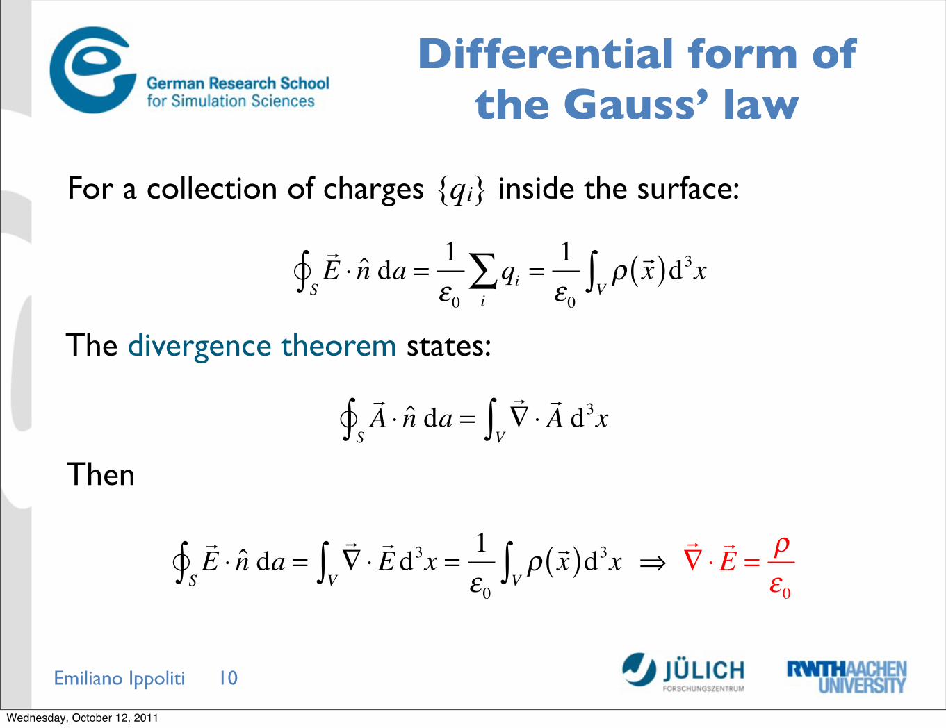
For a collection of charges {qi} inside the surface:

E ⋅ n da

S∫ =1ε0

qii∑ =

1ε0

ρ x( )d3xV∫

The divergence theorem states:

A ⋅ n da

S∫ =∇ ⋅A

V∫ d3x

Then

E ⋅ n da

S∫ =∇ ⋅E d3x

V∫ =1ε0

ρ x( )d3xV∫ ⇒

∇ ⋅E =

ρε0


Emiliano Ippoliti

Electrostatic potential

11

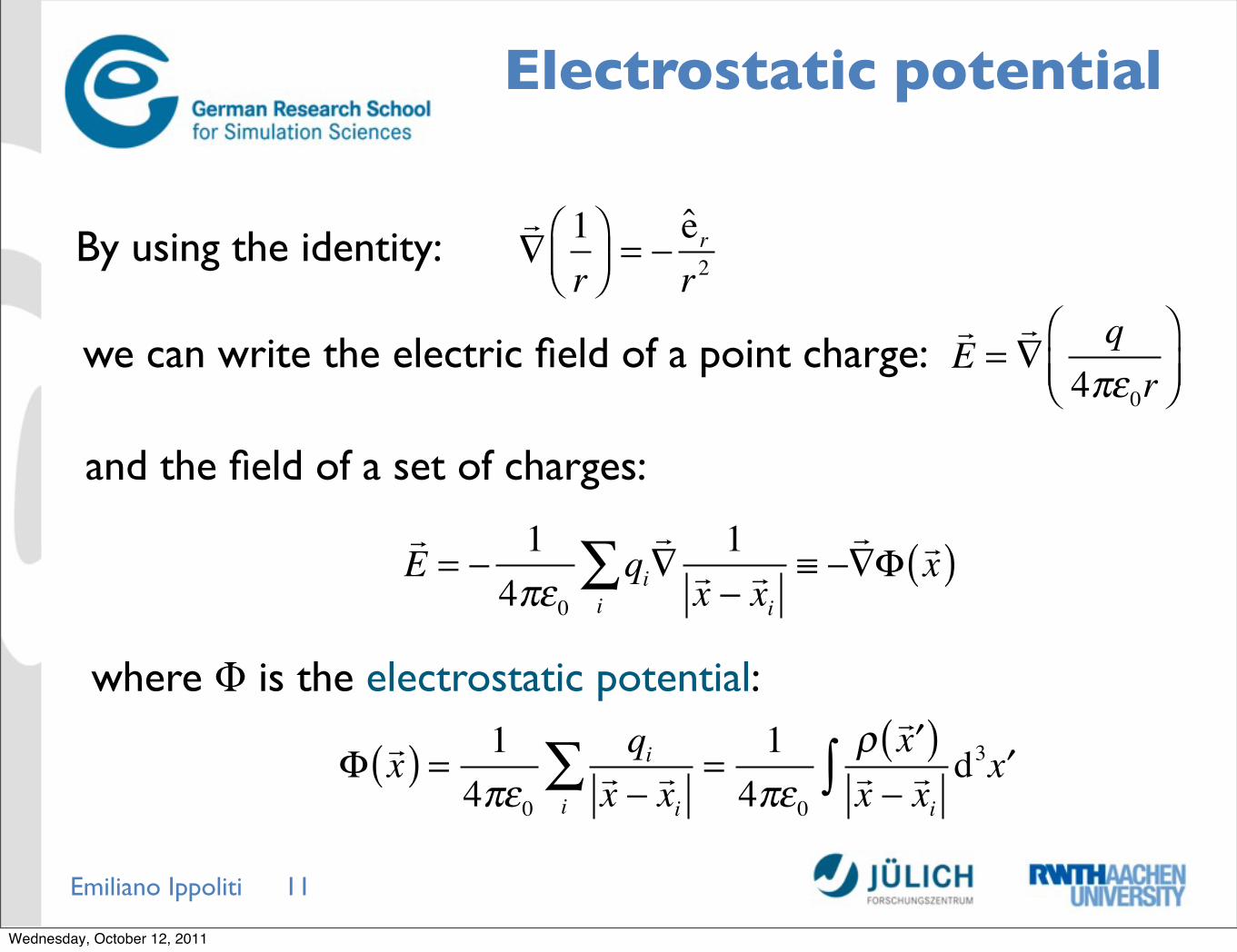
By using the identity:

∇1r

⎛⎝⎜

⎞⎠⎟= −

err2

we can write the electric field of a point charge:

E =∇

q4πε0r

⎛⎝⎜

⎞⎠⎟

and the field of a set of charges:

E = −

14πε0

qi∇

1x − xii

∑ ≡ −∇Φ x( )

where Φ is the electrostatic potential:

Φ x( ) = 1

4πε0qix − xii

∑ =14πε0

ρ ′x( )x − xi

d3 ′x∫


Emiliano Ippoliti

Meaning of Φ

12

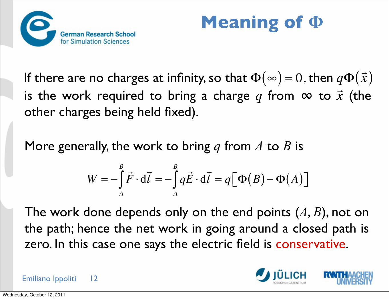
If there are no charges at infinity, so that Φ ∞( ) = 0, then qΦx( )

is the work required to bring a charge q from ∞ to x (the other charges being held fixed).

More generally, the work to bring q from A to B is

W = −

F ⋅dl

A

B

∫ = − qE ⋅dl

A

B

∫ = q Φ B( ) − Φ A( )⎡⎣ ⎤⎦

The work done depends only on the end points (A, B), not on the path; hence the net work in going around a closed path is zero. In this case one says the electric field is conservative.

x


Emiliano Ippoliti

Curl of the electric field

13

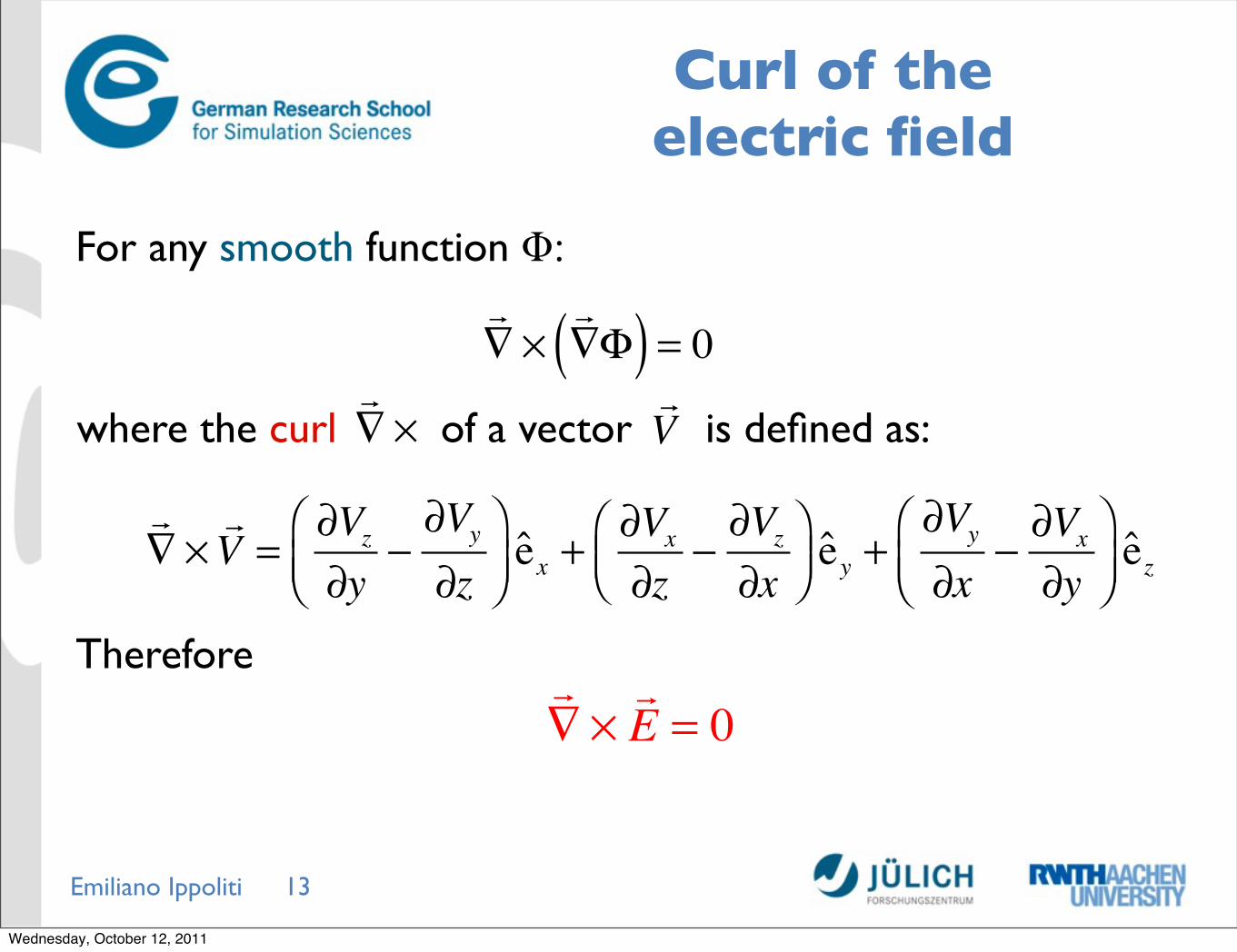
For any smooth function Φ:

∇ ×

∇Φ( ) = 0

where the curl ∇ × of a vector

V is defined as:

∇ ×V =

∂Vz∂y

−∂Vy∂z

⎛⎝⎜

⎞⎠⎟ex +

∂Vx∂z

−∂Vz∂x

⎛⎝⎜

⎞⎠⎟ey +

∂Vy∂x

−∂Vx∂y

⎛⎝⎜

⎞⎠⎟ez

Therefore

∇ ×E = 0


Emiliano Ippoliti

Stokes’ theorem

14

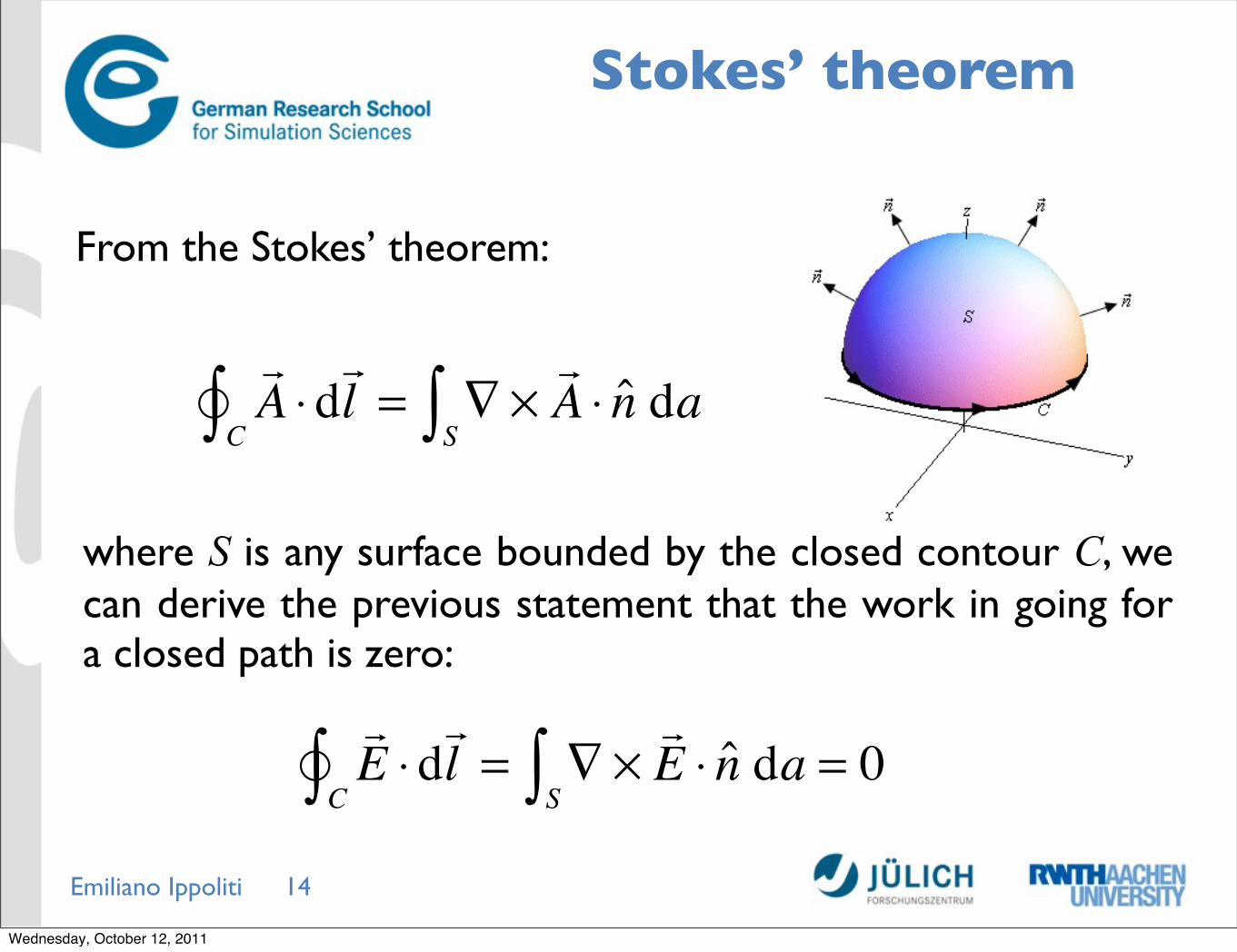
From the Stokes’ theorem:

where S is any surface bounded by the closed contour C, we can derive the previous statement that the work in going for a closed path is zero:

A ⋅dl

C∫ = ∇ ×A ⋅ n da

S∫

E ⋅dl

C∫ = ∇ ×E ⋅ n da

S∫ = 0


Emiliano Ippoliti

Lines of forces

15

The lines of force (also called the field lines) provide a method for graphing the electric field.

• They are everywhere tangent to the electric field and therefore for a point charge are tangent to the force exerted by the field on the particle.• They begin on positive charges and terminate on negative charges.• The local density of the field lines is proportional to the strength of the electric field.• The electric field lines do not cross (otherwise the field would not be unique at that point).

E

The lines of force are not particle trajectories! The particle trajectories are obtained by solving with .

F = ma

F = q

E


Emiliano Ippoliti

Lines of forcesExamples

16

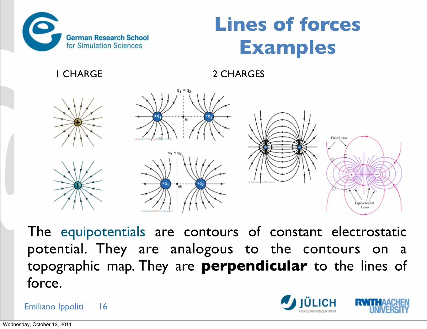
The equipotentials are contours of constant electrostatic potential. They are analogous to the contours on a topographic map. They are perpendicular to the lines of force.

1 CHARGE 2 CHARGES


Emiliano Ippoliti

Dipole

17

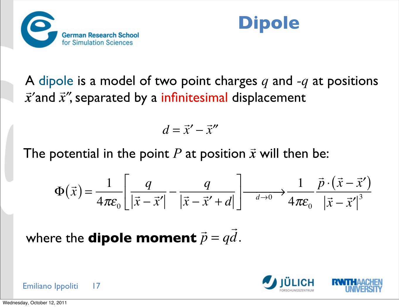
A dipole is a model of two point charges q and -q at positions x and x , separated by a infinitesimal displacement ′x

′′x

d = ′x − ′′x

The potential in the point P at position x will then be: x

Φ x( ) = 1

4πε0qx − ′x

−q

x − ′x + d⎡

⎣⎢

⎤

⎦⎥ d→0⎯ →⎯⎯

14πε0

p ⋅ x − ′x( )x − ′x 3

where the dipole moment p = q

d.


Emiliano Ippoliti

Dipole

18

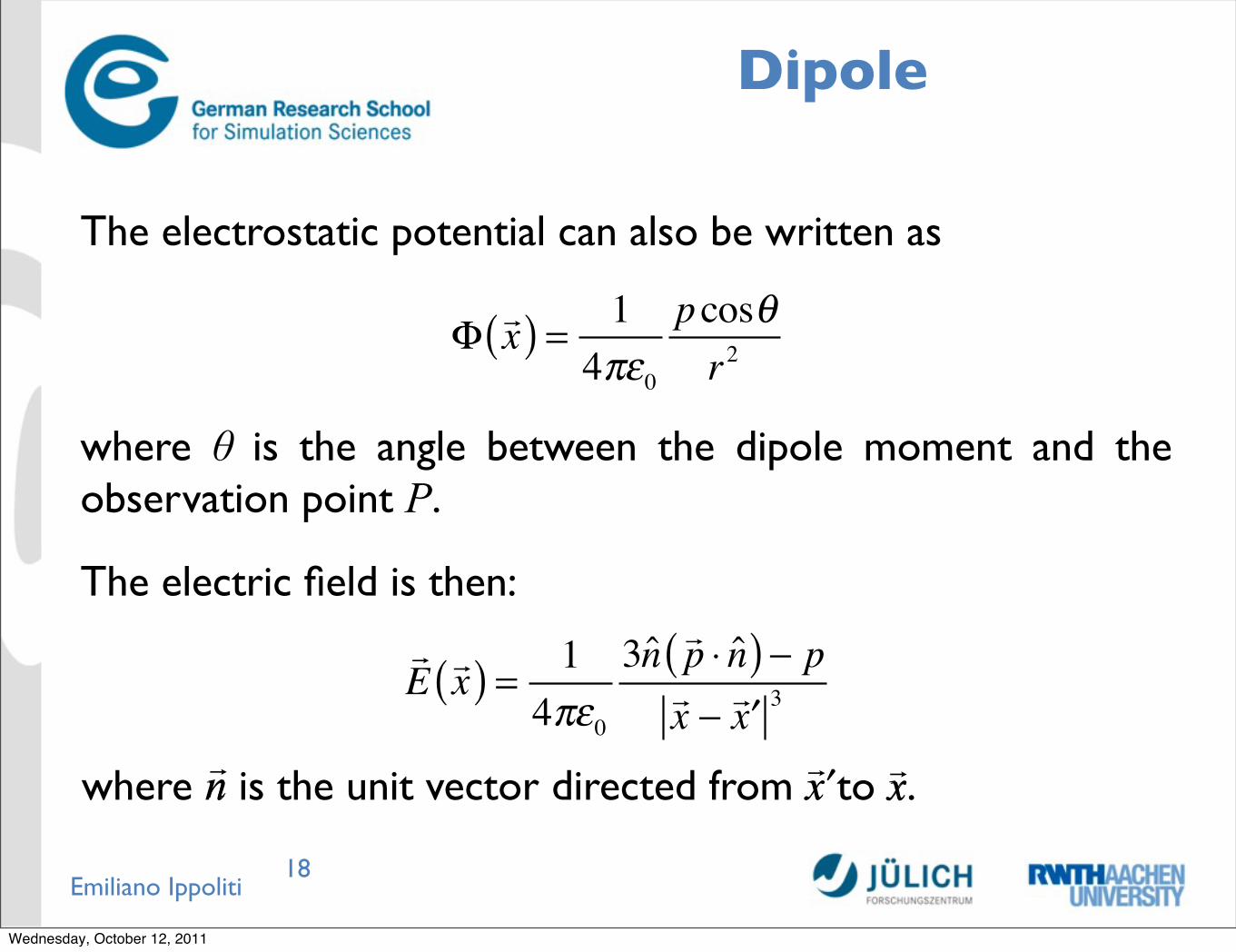
The electrostatic potential can also be written as

Φ x( ) = 1

4πε0pcosθr2

where θ is the angle between the dipole moment and the observation point P.

The electric field is then:

E x( ) = 1

4πε0

3n p ⋅ n( ) − px − ′x 3

where n is the unit vector directed from x to x. ′x

n x


Emiliano Ippoliti

Poisson equation

19

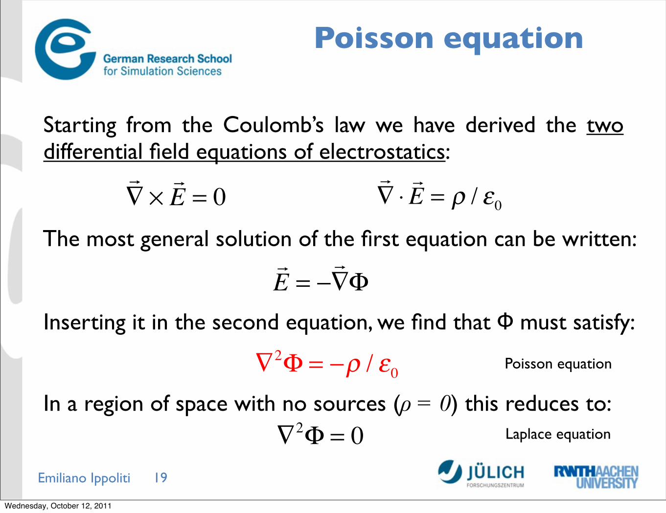
Starting from the Coulomb’s law we have derived the two differential field equations of electrostatics:

∇ ×E = 0

∇ ⋅E = ρ / ε0

The most general solution of the first equation can be written:

E = −

∇Φ

Inserting it in the second equation, we find that Φ must satisfy:

∇2Φ = −ρ / ε0 Poisson equation

In a region of space with no sources (ρ = 0) this reduces to:∇2Φ = 0 Laplace equation


Emiliano Ippoliti

References

20

1. A. Dorsey. Basic Electrostatics. http://www.phys.ufl.edu/~dorsey/phy6346-00/lectures/lect01.pdf 2. D.J. Griffiths. Introduction to Electrodynamics. 3th Eds. Benjamin Cummings, New Jersey, 1999.

3. J.D. Jackson. Classical Electrodynamics. 3th Eds. John Wiley & Son, New York, 1998.


http://www.phys.ufl.edu/~dorsey/phy6346-00/lectures/lect01.pdf




Basic Electrostatics - German Research School for ... Basic electrostatics • Classical...

Documents

Transcript of Basic Electrostatics - German Research School for ... Basic electrostatics • Classical...