Basic Concepts in Convexity and Computation - UC Davis …deloera/TEACHING/RM… · ·...
96
Crash Course on Combinatorial Convexity A Catalogue of famous and useful polytopes Crash Course on Computational Complexity Basic Concepts in Convexity and Computation Jes´ us A. De Loera, UC Davis June 19, 2011
Transcript of Basic Concepts in Convexity and Computation - UC Davis …deloera/TEACHING/RM… · ·...

Crash Course on Combinatorial ConvexityA Catalogue of famous and useful polytopesCrash Course on Computational Complexity
Basic Concepts in Convexity and Computation
Jesus A. De Loera, UC Davis
June 19, 2011

Crash Course on Combinatorial ConvexityA Catalogue of famous and useful polytopesCrash Course on Computational Complexity
Combinatorial Convexity

Crash Course on Combinatorial ConvexityA Catalogue of famous and useful polytopesCrash Course on Computational Complexity
Convexity I
Everything we do takes place inside Euclidean d-dimensionalspace Rd .
We have the traditional Euclidean inner-product, norm ofvectors, and distance between two points x , y defined by√
(x1 − y1)2 + . . . (x2 − y2)2.
The set of all points [x , y ] := {αx + (1− α)y : 0 ≤ α ≤ 1} iscalled the line segment between x and y . The points x and yare the endpoints of the interval.
A subset S of Rn is called convex if for any two distinct pointsx1, x2 in S the line segment joining x1, x2, lies completely in S .

Crash Course on Combinatorial ConvexityA Catalogue of famous and useful polytopesCrash Course on Computational Complexity
Convexity II
A linear functional f : Rd → R is given by a vectorc ∈ Rd , c 6= 0.
For a number α ∈ R we say that Hα = {x ∈ Rd : f (x) = α}is an affine hyperplane or hyperplane for short.
The intersection of finitely many hyperplanes is an affinespace. The affine hull of a set A is the smallest affine spacecontaining A.
Note that a hyperplane divides Rd into two halfspacesH+α = {x ∈ Rd : f (x) ≥ α} and H−α = {x ∈ Rd : f (x) ≤ α}.
Halfspaces are convex sets.

Crash Course on Combinatorial ConvexityA Catalogue of famous and useful polytopesCrash Course on Computational Complexity
Convexity III
The intersection of finitely many half-spaces is a polyhedron
Similarly: A polyhedron is then the set of solutions of asystem of linear inequalities
P = {x ∈ Rd :< ci , x >≤ βi},
for some non-zero vectors ci in Rd and some real numbers βi .
The intersection of convex sets is always convex. Let A ⊂ Rd ,the convex hull of A, denoted by conv(A), is the intersectionof all the convex sets containing A.
A polytope is the convex hull of a finite set of points in Rd . Itis the smallest convex set containing the points.
The image of a convex set under a linear transformation isagain a convex set.
Polyhedra and polytopes are always a convex sets!!
How are POLYTOPES and POLYHEDRA related?

Crash Course on Combinatorial ConvexityA Catalogue of famous and useful polytopesCrash Course on Computational Complexity
Convexity IV
Theorem: [Weyl-Minkowski] Every polytope is a polyhedron.Every bounded polyhedron is a polytope.
This allows us to represent all polytopes in two ways inside acomputer!! Either as a list of vertices, or as system ofinequalities.

Crash Course on Combinatorial ConvexityA Catalogue of famous and useful polytopesCrash Course on Computational Complexity
Convexity IV
Theorem: [Weyl-Minkowski] Every polytope is a polyhedron.Every bounded polyhedron is a polytope.This allows us to represent all polytopes in two ways inside acomputer!! Either as a list of vertices, or as system ofinequalities.

Crash Course on Combinatorial ConvexityA Catalogue of famous and useful polytopesCrash Course on Computational Complexity
Convexity V
Definition: Given finitely many points A := {x1, x2, . . . , xn}we say the linear combination
∑γixi is
an affine combination if∑γi = 1.
a convex combination if it is affine and γi ≥ 0 for all i .
Lemma: (EXERCISE) For a set of points A in Rd we havethat conv(A) equals all finite convex combinations of A:
conv(A) = {∑xi∈A
γixi : γi ≥ 0 and γ1 + . . . γk = 1}
Definition A set of points x1, . . . , xn is affinely dependent ifthere is a linear combination
∑aixi = 0 with
∑ai = 0.
Otherwise we say they are affinely independent.
Lemma: A set of d + 2 or more points in Rd is affinelydependent.

Crash Course on Combinatorial ConvexityA Catalogue of famous and useful polytopesCrash Course on Computational Complexity
Convexity VI
Here are three classical theorems about convex sets. We invite youto provide proofs for them (EXERCISE)!!
Theorem: (Caratheodory’s theorem): If x ∈ conv(S) ⊂ Rd ,then x is the convex combination of d + 1 points.
Theorem: (Radon’s theorem): If a set A with d + 2 points inRd then A can be partitioned into two sets X ,Y such thatconv(X ) ∩ conv(Y ) 6= ∅.Theorem: (Helly’s theorem): If C is a collection of closedbounded convex sets in Rd such that each d + 1 sets havenonempty intersection then the intersection of all sets in C isnon-empty.

Crash Course on Combinatorial ConvexityA Catalogue of famous and useful polytopesCrash Course on Computational Complexity
Convexity VI
Here are three classical theorems about convex sets. We invite youto provide proofs for them (EXERCISE)!!
Theorem: (Caratheodory’s theorem): If x ∈ conv(S) ⊂ Rd ,then x is the convex combination of d + 1 points.
Theorem: (Radon’s theorem): If a set A with d + 2 points inRd then A can be partitioned into two sets X ,Y such thatconv(X ) ∩ conv(Y ) 6= ∅.
Theorem: (Helly’s theorem): If C is a collection of closedbounded convex sets in Rd such that each d + 1 sets havenonempty intersection then the intersection of all sets in C isnon-empty.

Crash Course on Combinatorial ConvexityA Catalogue of famous and useful polytopesCrash Course on Computational Complexity
Convexity VI
Here are three classical theorems about convex sets. We invite youto provide proofs for them (EXERCISE)!!
Theorem: (Caratheodory’s theorem): If x ∈ conv(S) ⊂ Rd ,then x is the convex combination of d + 1 points.
Theorem: (Radon’s theorem): If a set A with d + 2 points inRd then A can be partitioned into two sets X ,Y such thatconv(X ) ∩ conv(Y ) 6= ∅.Theorem: (Helly’s theorem): If C is a collection of closedbounded convex sets in Rd such that each d + 1 sets havenonempty intersection then the intersection of all sets in C isnon-empty.

Crash Course on Combinatorial ConvexityA Catalogue of famous and useful polytopesCrash Course on Computational Complexity
Convexity VI
For a convex set S in Rd . A linear inequality f (x) ≤ α is saidto be valid on S if every point in P satisfies it.
A set F ⊂ S is a face of P if and only there exists a linearinequality f (x) ≤ α which is valid on P and such thatF = {x ∈ P : f (x) = α}. Then the hyperplane defined by f isa supporting hyperplane of F .
The dimension of an affine set is the largest number ofaffinely independent points in the set minus one. Thedimension of a set in Rd is the dimension of its affine hull.
A face of dimension 0 is called a vertex. A face of dimension 1is called an edge, and a face of dimension dim(P)− 1 is calleda facet. The empty set is defined to be a face of P ofdimension −1. Faces that are not the empty set or P itself arecalled proper.

Crash Course on Combinatorial ConvexityA Catalogue of famous and useful polytopesCrash Course on Computational Complexity
Convexity VII
Theorem: The set of of faces of a polyhedron (polytope)forms also a finite poset by containment.
For any d-polytope, denote by fi (P) the number of i-faces ofP. The f-vector of P is
f (P) = (f0(P), f1(P), . . . , fd−1(P)).
Theorem (Euler-Poincare formula) For any d-dimensionalPolytope P, then
d∑i=−1
(−1)i fi (P) = 0
Theorem (Upper bound theorem) For any d-polytope P withn vertices has no
fi (P) ≤ fi (C (n, d))
Where C (n, d) is a special polytope, the cyclic polytope. Inparticular fd−1(P) ≤ O(nbd/2c).

Crash Course on Combinatorial ConvexityA Catalogue of famous and useful polytopesCrash Course on Computational Complexity
Convexity VII
Theorem: The set of of faces of a polyhedron (polytope)forms also a finite poset by containment.For any d-polytope, denote by fi (P) the number of i-faces ofP. The f-vector of P is
f (P) = (f0(P), f1(P), . . . , fd−1(P)).
Theorem (Euler-Poincare formula) For any d-dimensionalPolytope P, then
d∑i=−1
(−1)i fi (P) = 0
Theorem (Upper bound theorem) For any d-polytope P withn vertices has no
fi (P) ≤ fi (C (n, d))
Where C (n, d) is a special polytope, the cyclic polytope. Inparticular fd−1(P) ≤ O(nbd/2c).
Crash Course on Combinatorial ConvexityA Catalogue of famous and useful polytopesCrash Course on Computational Complexity
Convexity VIII
Definition: Two polytopes are combinatorially isomorphic iftheir face posets are the same.
It follows: two polytopes P,Q are isomorphic if there is aone-to-one correspondence pi to qi between the vertices suchthat conv(pi : i ∈ I ) is a face of P if and only ifconv(qi : i ∈ I ) is a face of Q.
Definition: The graph of a polytope (or polyhedron) is thegraph given of 1-dimensional faces (edges) and the vertices(0-dimensional faces).
Theorem: (Balinski’s theorem) The graphs of d-dimensionalpolytopes are always d-connected.
QUESTION: How can we compute the faces of a polyhedron?

Crash Course on Combinatorial ConvexityA Catalogue of famous and useful polytopesCrash Course on Computational Complexity
Convexity IX
For A ⊂ Rd polar of A is
Ao = {x ∈ Rd :< x , a >≤ 1 for every a ∈ A}
Another way of thinking of the polar is as the intersection ofthe halfspaces, one for each element a ∈ A, of the form
{x ∈ Rd :< x , a >≤ 1}
Example 1: Take L a line in R2 passing through the origin,what is Lo? the perpendicular line that passes through theorigin.
Example 2: If the line L does not pass through the originthen, Lo is a clipped line orthogonal to the given line thatpasses through the origin.

Crash Course on Combinatorial ConvexityA Catalogue of famous and useful polytopesCrash Course on Computational Complexity
Convexity IX
For A ⊂ Rd polar of A is
Ao = {x ∈ Rd :< x , a >≤ 1 for every a ∈ A}
Another way of thinking of the polar is as the intersection ofthe halfspaces, one for each element a ∈ A, of the form
{x ∈ Rd :< x , a >≤ 1}
Example 1: Take L a line in R2 passing through the origin,what is Lo?
the perpendicular line that passes through theorigin.
Example 2: If the line L does not pass through the originthen, Lo is a clipped line orthogonal to the given line thatpasses through the origin.

Crash Course on Combinatorial ConvexityA Catalogue of famous and useful polytopesCrash Course on Computational Complexity
Convexity IX
For A ⊂ Rd polar of A is
Ao = {x ∈ Rd :< x , a >≤ 1 for every a ∈ A}
Another way of thinking of the polar is as the intersection ofthe halfspaces, one for each element a ∈ A, of the form
{x ∈ Rd :< x , a >≤ 1}
Example 1: Take L a line in R2 passing through the origin,what is Lo? the perpendicular line that passes through theorigin.
Example 2: If the line L does not pass through the originthen,
Lo is a clipped line orthogonal to the given line thatpasses through the origin.

Crash Course on Combinatorial ConvexityA Catalogue of famous and useful polytopesCrash Course on Computational Complexity
Convexity IX
For A ⊂ Rd polar of A is
Ao = {x ∈ Rd :< x , a >≤ 1 for every a ∈ A}
Another way of thinking of the polar is as the intersection ofthe halfspaces, one for each element a ∈ A, of the form
{x ∈ Rd :< x , a >≤ 1}
Example 1: Take L a line in R2 passing through the origin,what is Lo? the perpendicular line that passes through theorigin.
Example 2: If the line L does not pass through the originthen, Lo is a clipped line orthogonal to the given line thatpasses through the origin.

Crash Course on Combinatorial ConvexityA Catalogue of famous and useful polytopesCrash Course on Computational Complexity
Convexity IX
For A ⊂ Rd polar of A is
Ao = {x ∈ Rd :< x , a >≤ 1 for every a ∈ A}
Another way of thinking of the polar is as the intersection ofthe halfspaces, one for each element a ∈ A, of the form
{x ∈ Rd :< x , a >≤ 1}
Example 1: Take L a line in R2 passing through the origin,what is Lo? the perpendicular line that passes through theorigin.
Example 2: If the line L does not pass through the originthen, Lo is a clipped line orthogonal to the given line thatpasses through the origin.

Crash Course on Combinatorial ConvexityA Catalogue of famous and useful polytopesCrash Course on Computational Complexity
Convexity X
Theorem For any polytope P, there is a polytope P∗, a polarpolytope of P, whose face lattice is isomorphic to the reversedposet of the face lattice of P.
idea of proof: Translate P ⊂ Rd to contain the origin as itsinterior point. For a non-empty face F of P define
F = {x ∈ Po :< x , y >= 1for all y ∈ F}
and for the empty face defineˆ= P0.The hat operation applied to faces of a d-polytope P satisfies
1 The set F is a face of Po
2 dim(F ) + dim(F ) = d − 1.
3 The hat operation is involutory: ˆF = F .4 If F ,G ⊂ P are faces and F ⊂ G ⊂ P, then G , F are faces of
Po and G ⊂ F .

Crash Course on Combinatorial ConvexityA Catalogue of famous and useful polytopesCrash Course on Computational Complexity
A few key examples to play...
Crash Course on Combinatorial ConvexityA Catalogue of famous and useful polytopesCrash Course on Computational Complexity
Simplices
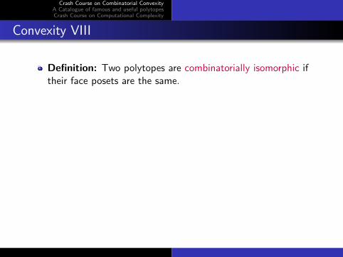
Let e1, e2, . . . , ed+1 be the standard unit vectors in Rd+1. Thestandard d-dimensional simplex ∆d is conv({e1, . . . , ed+1}).Thus∆d = {x = (x1, . . . , xd+1) : xi ≥ 0 and x1 + x2 + · · ·+ xd+1 =1}.Note that for polytope P = conv({a1, . . . , am}) we can definea linear map f : ∆m−1 → P by the formulaf (λ1, . . . , λm) = λ1a1 + · · ·+ λmam. Thus f (∆m−1) = P.Every polytope is the image of the standard simplex under alinear transformation.

Crash Course on Combinatorial ConvexityA Catalogue of famous and useful polytopesCrash Course on Computational Complexity
Cubes and Zonotopes
Let {ui : i ∈ I} be the set of all 2d vectors in Rd whosecoordinates are either 1 or -1.
The polytope Id = conv({ui : i ∈ I} is called the standard unitd-dimensional cube. Thus I d = {(x1, . . . , xd) : −1 ≤ xi ≤ 1}.The images of a cube under linear transformations receive thename of zonotopes.

Crash Course on Combinatorial ConvexityA Catalogue of famous and useful polytopesCrash Course on Computational Complexity
Birkhoff’s polytope
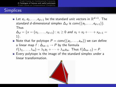
Let Bn be the convex polytope of real non-negative matriceswith all row and column sums equal to one (doubly-stochasticmatrices). The dimension of Bn is (n − 1)2.The polytope Bn is called the Birkhoff polytope, theassignment polytope, or the Birkhoff-von Neumann polytope.
Graph of Bn: The vertices of Bn are the n × n permutationmatrices. The edges of Bn correspond to cycles in thecomplete bipartite Kn,n. Its graph has diameter 2.
Facets: For each pair (i , j) with 1 ≤ i , j ≤ n, the doublystochastic matrices with (i , j) entry equal to 0 is a facet(maximal proper face) of Bn and all facets arise in this way.
The linear projection of Bn given by multiplying each matrixby a vector v gives a Permutahedron.

Crash Course on Combinatorial ConvexityA Catalogue of famous and useful polytopesCrash Course on Computational Complexity
Birkhoff’s polytope
Let Bn be the convex polytope of real non-negative matriceswith all row and column sums equal to one (doubly-stochasticmatrices). The dimension of Bn is (n − 1)2.The polytope Bn is called the Birkhoff polytope, theassignment polytope, or the Birkhoff-von Neumann polytope.
Graph of Bn: The vertices of Bn are the n × n permutationmatrices. The edges of Bn correspond to cycles in thecomplete bipartite Kn,n. Its graph has diameter 2.
Facets: For each pair (i , j) with 1 ≤ i , j ≤ n, the doublystochastic matrices with (i , j) entry equal to 0 is a facet(maximal proper face) of Bn and all facets arise in this way.
The linear projection of Bn given by multiplying each matrixby a vector v gives a Permutahedron.

Crash Course on Combinatorial ConvexityA Catalogue of famous and useful polytopesCrash Course on Computational Complexity
Cyclic Polytopes
The moment curve is a curve parametrized as follows:γ(t) = (t, t2, t3, . . . , td).
definition Take n different values for t. That gives n differentpoints in the curve. The cyclic polytope C (n, d) is the convexhull of such points.
Lemma: Every hyperplane intersects the moment curveγ(t) = (t, t2, t3, . . . , td) in no more than d points.
Theorem: The largest possible number of i-dimensional facesof a d-polytope with n vertices is achieved by the cyclicpolytope C (n, d).

Crash Course on Combinatorial ConvexityA Catalogue of famous and useful polytopesCrash Course on Computational Complexity
Computational Complexity

Crash Course on Combinatorial ConvexityA Catalogue of famous and useful polytopesCrash Course on Computational Complexity
Computational Complexity
We need a theory to measure how difficult is to compute!!!
The study of the efficiency of algorithms and the difficulty ofproblems.
Problem: a generic computational question that can bestated without any data specificied.
Examples:
Clique: Given a graph G = (V ,E ) and an integer k, does Ghave a clique of size k?
An instance of a problem is a particular specification of thedata.
Examples:
Does the Peterson graph have a clique of size 4?

Crash Course on Combinatorial ConvexityA Catalogue of famous and useful polytopesCrash Course on Computational Complexity
Computational Complexity
We need a theory to measure how difficult is to compute!!!
The study of the efficiency of algorithms and the difficulty ofproblems.
Problem: a generic computational question that can bestated without any data specificied.
Examples:Clique: Given a graph G = (V ,E ) and an integer k, does Ghave a clique of size k?
An instance of a problem is a particular specification of thedata.
Examples:Does the Peterson graph have a clique of size 4?

Crash Course on Combinatorial ConvexityA Catalogue of famous and useful polytopesCrash Course on Computational Complexity
Algorithms
An algorithm is a finite set of instructions for performing basicoperations on an input to produce an output.
An algorithm A solves a problem P if given a representationof each instance I as input it supplies as output the solutionof instance I .
Instances can have more than one representation.
A graph G = (V ,E ) can be represented as a adjacency matrix,incidence matrix, adjacency list, etc.

Crash Course on Combinatorial ConvexityA Catalogue of famous and useful polytopesCrash Course on Computational Complexity
Running time
Question: How to measure the efficiency of an algorithm A?
Answer: Running time - count of the number of elementaryoperations needed to run the algorithm.
Key insight: the number of operations depends on thedifficulty of the instance and the size of the input.
Worst case difficulty: consider run times of “hard” instances.Express run time as a function of the amount of “memory”needed to represent the instance!

Crash Course on Combinatorial ConvexityA Catalogue of famous and useful polytopesCrash Course on Computational Complexity
Running time
Question: How to measure the efficiency of an algorithm A?
Answer: Running time - count of the number of elementaryoperations needed to run the algorithm.
Key insight: the number of operations depends on thedifficulty of the instance and the size of the input.
Worst case difficulty: consider run times of “hard” instances.
Express run time as a function of the amount of “memory”needed to represent the instance!
Crash Course on Combinatorial ConvexityA Catalogue of famous and useful polytopesCrash Course on Computational Complexity
Running time
Question: How to measure the efficiency of an algorithm A?
Answer: Running time - count of the number of elementaryoperations needed to run the algorithm.
Key insight: the number of operations depends on thedifficulty of the instance and the size of the input.
Worst case difficulty: consider run times of “hard” instances.Express run time as a function of the amount of “memory”needed to represent the instance!

Crash Course on Combinatorial ConvexityA Catalogue of famous and useful polytopesCrash Course on Computational Complexity
Binary encoding size of an instance
The size of an instance depends on its representation.
The encoding size of a representation is the number of binarydigits (bits) needed to encode it into memory.
Some examples of binary encoding sizes:
1 n = 118.
n = 64 + 32 + 16 + 4 + 2
= 110110 (in binary)
That is, |n| = 7 bitsMore generally, n ∈ Z can be encoded in around log2 n bits.
2 The set S = {0, . . . , n} can also be encoded in around log2 nbits.

Crash Course on Combinatorial ConvexityA Catalogue of famous and useful polytopesCrash Course on Computational Complexity
Binary encoding size of an instance
The size of an instance depends on its representation.
The encoding size of a representation is the number of binarydigits (bits) needed to encode it into memory.
Some examples of binary encoding sizes:1 n = 118.
n = 64 + 32 + 16 + 4 + 2
= 110110 (in binary)
That is, |n| = 7 bits
More generally, n ∈ Z can be encoded in around log2 n bits.2 The set S = {0, . . . , n} can also be encoded in around log2 n
bits.

Crash Course on Combinatorial ConvexityA Catalogue of famous and useful polytopesCrash Course on Computational Complexity
Binary encoding size of an instance
The size of an instance depends on its representation.
The encoding size of a representation is the number of binarydigits (bits) needed to encode it into memory.
Some examples of binary encoding sizes:1 n = 118.
n = 64 + 32 + 16 + 4 + 2
= 110110 (in binary)
That is, |n| = 7 bitsMore generally, n ∈ Z can be encoded in around log2 n bits.
2 The set S = {0, . . . , n} can also be encoded in around log2 nbits.

Crash Course on Combinatorial ConvexityA Catalogue of famous and useful polytopesCrash Course on Computational Complexity
Binary encoding size of an instance
The size of an instance depends on its representation.
The encoding size of a representation is the number of binarydigits (bits) needed to encode it into memory.
Some examples of binary encoding sizes:1 n = 118.
n = 64 + 32 + 16 + 4 + 2
= 110110 (in binary)
That is, |n| = 7 bitsMore generally, n ∈ Z can be encoded in around log2 n bits.
2 The set S = {0, . . . , n} can also be encoded in around log2 nbits.

Crash Course on Combinatorial ConvexityA Catalogue of famous and useful polytopesCrash Course on Computational Complexity
Polynomial time algorithms
If the running time of an algorithm is bounded by apolynomial function of the input size, then we say thealgorithm runs in polynomial time.
For example: ordering a finite list L of numbers
Input size of the normal form representation of L is the size n.
Silly algorithm requires around(n2
)comparisons and
re-ordering of the lists.

Crash Course on Combinatorial ConvexityA Catalogue of famous and useful polytopesCrash Course on Computational Complexity
P vs NP: What you need to know
What do you mean is HARD TO COMPUTE X ??
Figure: I tried to compute X, I can’t do it, therefore it must be hard!
Crash Course on Combinatorial ConvexityA Catalogue of famous and useful polytopesCrash Course on Computational Complexity
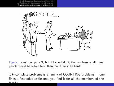
Figure: I can’t compute X, but if I could do it, the problems of all thesepeople would be solved too! therefore it must be hard!
#P-complete problems is a family of COUNTING problems, if onefinds a fast solution for one, you find it for all the members of thefamily!

Crash Course on Combinatorial ConvexityA Catalogue of famous and useful polytopesCrash Course on Computational Complexity
Many of the problems we care about require LISTING all theelements of a set: e.g., list all facets, all vertices. There are nouniformly accepted complexity notions for LISTING algorithms,and the output size can be LARGE.
An algorithm is output sensitive if it runs in TIME polynomialin both the input size and the output size.
An algorithm is compact if it runs in SPACE polynomial in theinput size ONLY.An ideal listing algorithm is a compact output-sensitivealgorithm. Hard to find!!!

Crash Course on Combinatorial ConvexityA Catalogue of famous and useful polytopesCrash Course on Computational Complexity
Thank you