Baseline eco-efficiency assessment for the analysed...
67
Meso-level eco-efficiency indicators to assess technologies and their uptake in water use sectors Collaborative project, Grant Agreement No: 282882 Deliverable 2.2 Baseline eco-efficiency assessment for the analysed agricultural water systems April 2014
Transcript of Baseline eco-efficiency assessment for the analysed...

Meso-level eco-efficiency indicators to assess
technologies and their uptake in water use sectors
Collaborative project, Grant Agreement No: 282882
Deliverable 2.2
Baseline eco-efficiency assessment for the
analysed agricultural water systems
April 2014
DOCUMENT INFORMATION
Project
Project acronym: EcoWater
Project full title: Meso-level eco-efficiency indicators to assess
technologies and their uptake in water use sectors
Grant agreement no.: 282882
Funding scheme: Collaborative Project
Project start date: 01/11/2011
Project duration: 36 months
Call topic: ENV.2011.3.1.9-2: Development of eco-efficiency
meso-level indicators for technology assessment
Project web-site: http://environ.chemeng.ntua.gr/ecowater
Document
Deliverable number: Deliverable 2.2
Deliverable title: Baseline eco-efficiency assessment in agricultural
water systems
Due date of deliverable: 31 October 2013
Actual submission date: 08 April 2014
Editor(s): CIHEAM-IAMB
Author(s): CIHEAM-IAMB, UPORTO
Reviewer(s): NTUA
Work Package no.: WP2
Work Package title: Eco-efficiency assessments in agricultural water
systems and use
Work Package Leader: Centro Internazionale di Alti Studi Agronomici
Mediterranei – Istituto Agronomico Mediterraneo di
Bari
Dissemination level: Public
Version: 2
Draft/Final: Final
No of pages (including cover): 67
Keywords: Eco-efficiency assessment, Agricultural Water Use
D2.2 Baseline eco-efficiency assessment for the analysed agricultural water systems Page 3 of 67
Abstract
This document delivers the results of baseline meso-level eco-efficiency assessment
of Sinistra Ofanto irrigation scheme (CS1) and the Monte Novo Irrigation Scheme
(CS2). The methodological approach followed is the same in both case studies.
Inventory analysis is used for data collection to estimate all the inputs (resources)
and outputs (emissions) in relation to the functional unit. The input and output data
include the use of resources (water, energy, fuel and N and P fertilizers) and the
releases to air, soil and water associated with the processes. Two types of data are
gathered for each unit process: environmental flows and economic flows.
For the Sinistra Ofanto irrigation scheme, the assessment was performed for two
different cases; normal and dry year, corresponding to annual precipitation of 514
and 420 mm, respectively. The on-field agronomic and water management practices,
water delivery and economic data refer to year 2007. Hence, the baseline scenario
adopts the application of deficit irrigation strategy for artichoke, olives, orchards and
sugarbeet, and full irrigation for other crops except wheat which was grown under
rainfed conditions.
The eco-efficiency was estimated as a ratio between the economic performances of
the system and produced environmental impacts. Economic performance was
expressed in terms of the Total Value Added from the water use and adopted
management practices, whereas the environmental performance referred to 11
midpoint environmental impact categories which were selected as the more
representative for the environmental assessment of the system. The analysis was
performed by using the Environmental Analysis Tool (SEAT) and Economic Value
chain Analysis Tool (EVAT), both developed in EcoWater project. The environmental
impacts analysis on a cluster (crop) level is performed on the basis of the irrigation
(water) supply to crops and corresponding agronomic practices.

D2.2 Baseline eco-efficiency assessment for the analysed agricultural water systems Page 4 of 67
Table of Contents
1 Baseline eco-efficiency assessment of the Sinistra Ofanto Irrigation Scheme, Italy .......................................................................................................... 11
1.1 Goal and scope definition .......................................................................... 11
1.1.1 Objectives .......................................................................................... 11
1.1.2 System Boundaries ............................................................................ 11
1.1.3 Functional unit .................................................................................... 13
1.2 Inventory Analysis ..................................................................................... 14
1.2.1 Elementary Flows .............................................................................. 14
1.3 Resource modeling and data input ............................................................ 14
1.3.1 Water service related materials .......................................................... 15
1.3.2 Supplementary Resources ................................................................. 17
1.3.3 Emissions to Air and Water ................................................................ 19
1.3.4 Water to Aquifer Recharge, Surface Recharge and Evaporation ........ 22
1.3.5 Products ............................................................................................. 23
1.4 Economic Data .......................................................................................... 24
1.4.1 Total Value Added and Financial Costs .............................................. 24
1.4.2 Water tariffs........................................................................................ 25
1.5 Baseline eco-efficiency assessment .......................................................... 25
1.5.1 Calculated life cycle inventory flows (Normal Hydrological Year)........ 25
1.5.2 Calculated life cycle inventory flows (Dry Year) .................................. 29
1.5.3 Environmental Impact Assessment of the Entire System.................... 31
1.5.4 Economic performance assessment .................................................. 38
1.6 Eco-efficiency indicators ............................................................................ 40
1.7 Conclusions .............................................................................................. 41
2 Baseline eco-efficiency assessment of the Monte Novo Case Study ....... 43
2.1 Introduction ............................................................................................... 43
2.2 Goal and Scope Definition ......................................................................... 43
2.2.1 Objectives .......................................................................................... 43
2.2.2 System boundaries ............................................................................ 44
2.2.3 Function unit definition ....................................................................... 47
2.3 Environmental Assessment ....................................................................... 47
2.3.1 Inventory analysis .............................................................................. 48
2.3.2 Impact Assessment ............................................................................ 49
2.3.3 Environmental impact categories ....................................................... 49
2.4 Value Assessment .................................................................................... 57
2.5 Eco-Efficiency Quantification ..................................................................... 58
2.6 Conclusions .............................................................................................. 58

D2.2 Baseline eco-efficiency assessment for the analysed agricultural water systems Page 5 of 67
3 References .............................................................................................. 60
Annex A - The results of environmental impact indicators at cluster level for a normal hydrological year ..................................................................................................... 62
D2.2 Baseline eco-efficiency assessment for the analysed agricultural water systems Page 6 of 67
List of tables
Table 1. Foreground and Background processes of the Sinistra Ofanto Irrigation Scheme ................................................................................................................ 13
Table 2. Resources of Sinistra Ofanto agricultural water system ............................. 14
Table 3. Water losses in different delivery stages of SO scheme ............................ 15
Table 4. Seasonal ETc, Peff, and NIR for average and dry year conditions ............. 16
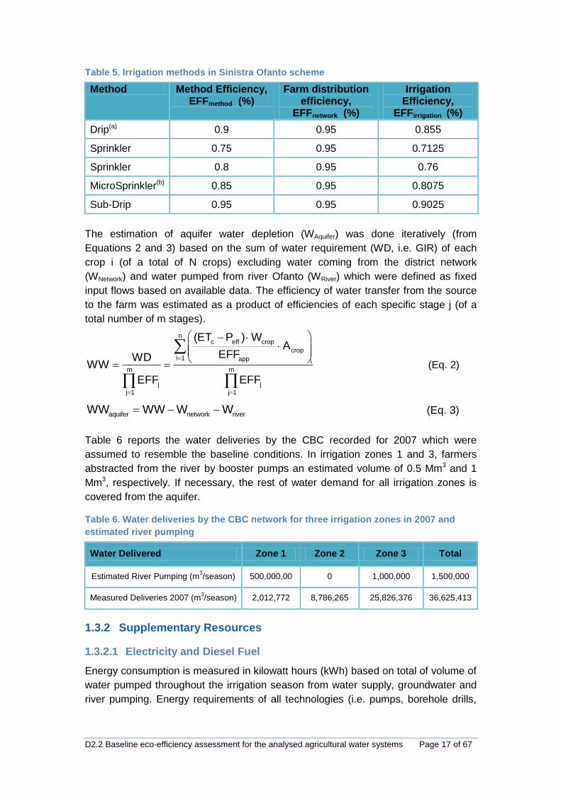
Table 5. Irrigation methods in Sinistra Ofanto scheme ............................................ 17
Table 6. Water deliveries by the CBC network for three irrigation zones in 2007 and estimated river pumping .......................................................................................... 17
Table 7. Energy requirements in the water supply chain (CBC, and pumping from river and from aquifer) ............................................................................................. 18
Table 8. Recommended Nitrogen and Phosphorus requirements for the crops in the CS ................................................................................................................ 18
Table 9. Crop distribution [ha] in the sub-schemes of the CS area for the baseline . 18
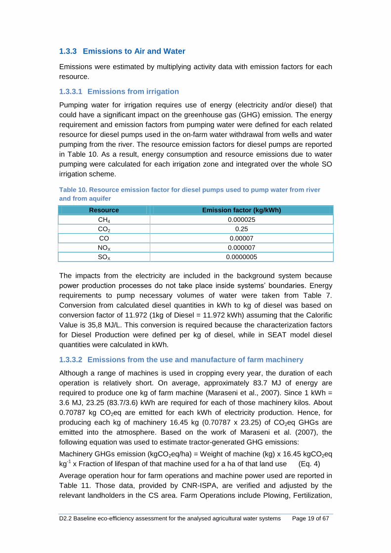
Table 10. Resource emission factor for diesel pumps used to pump water from river and from aquifer ...................................................................................................... 19
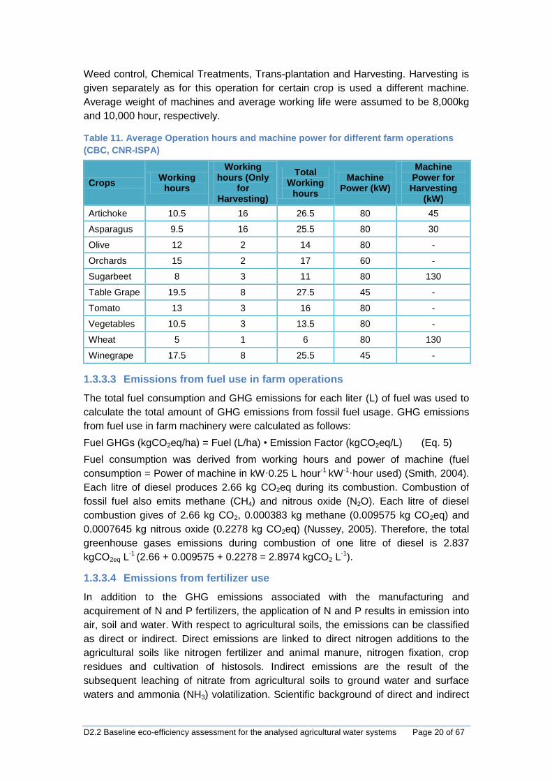
Table 11. Average Operation hours and machine power for different farm operations (CBC, CNR-ISPA) ................................................................................................... 20
Table 12. Low, average, and high emission factors used for estimating N2O emissions from N fertilizer and lime using IPCC (Eggleston et al., 2006) guidelines. 21
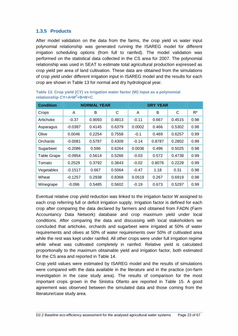
Table 13. Crop yield (CY) vs irrigation water factor (W) input as a polynomial relationship CY=A•W2+B•W+C ............................................................................... 23
Table 14. Crop yield declared for FADN 2007, maximum obtainable yield under local condition and irrigation factor (W) defined for each crop. ......................................... 24
Table 15. Simulated and observed crop yield values (t/ha)...................................... 24
Table 16. Gross Market Price and production cost (FADN, 2007) ........................... 25
Table 17. Life cycle inventory flows of the Sinistra Ofanto Irrigation Scheme (2007, a normal hydrological year) ........................................................................................ 27
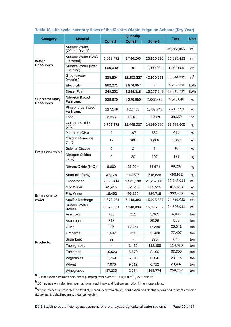
Table 18. Life cycle inventory flows of the Sinistra Ofanto Irrigation Scheme (Dry Year) ................................................................................................................ 30
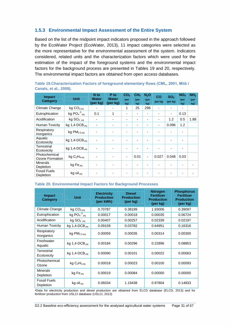
Table 19.Characterization Factors of foreground elementary flows (CML, 2001, Milà i Canals, et al., 2009). ............................................................................................... 31
Table 20. Environmental Impact Factors for Background Processes ....................... 31
Table 21. Environmental Impacts of the Study System (Normal Hydrological Year) 33
Table 22. Environmental Impacts of the Study System (Dry Year) .......................... 36
Table 23. Economic performance results (Normal Hydrological Year) ..................... 38
Table 24. Economic performance results (Dry Year) ............................................... 39
Table 25. Eco-efficiency indicators for the baseline scenario of Sinistra Ofanto agricultural water system ......................................................................................... 41
Table 26. Stages, processes and technologies in the Monte Novo case study. ....... 44
Table 27. Foreground and Background processes of the Monte Novo Irrigation Scheme. ................................................................................................................ 46
D2.2 Baseline eco-efficiency assessment for the analysed agricultural water systems Page 7 of 67
Table 28. Function unit definition according to two different approaches. ................ 47
Table 29. Resources of the Monte Novo case study................................................ 48
Table 30. Life cycle inventory flows of the Monte Novo Irrigation Scheme (from SEAT). ................................................................................................................ 49
Table 31. Unit costs of raw materials and supplementary resources. ...................... 49
Table 32. Midpoint impact categories and impact assessment methods. ................. 50
Table 33. Characterization factors of foreground elementary flows. ........................ 50
Table 34. Background processes and relevant data sources. .................................. 51
Table 35. Environmental impact factors for background processes. ........................ 51
Table 36. Environmental impacts from foreground and background systems. ......... 52
Table 37. Financial summary per actor. ................................................................... 57
Table 38. Eco-efficiency indicators. ......................................................................... 58
D2.2 Baseline eco-efficiency assessment for the analysed agricultural water systems Page 8 of 67
List of figures
Figure 1. Stages and involved actors in the water value chain of the Sinistra Ofanto Irrigation Scheme .................................................................................................... 11
Figure 2. Foreground and background systems ...................................................... 12
Figure 3. Simplified soil-water-balance .................................................................... 15
Figure 4. Simplified concept of N and P balances ................................................... 21
Figure 5. Greenhouse gas emissions from farm supplementary resources in Sinistra Ofanto irrigation scheme ......................................................................................... 28
Figure 6. Contribution of Foreground and Background Systems in the environmental impact categories for normal year conditions .......................................................... 33
Figure 7. Environmental Impact Breakdown, percentage per stage (1/2) ................. 34
Figure 8. Environmental Impact Breakdown, percentage per stage (2/2) ................. 35
Figure 9. Contribution of Foreground and Background Systems in the environmental impact categories for dry year conditions ................................................................ 36
Figure 10. Environmental Impact Breakdown, percentage per stage (1/2) - Dry Year .. ................................................................................................................ 37
Figure 11. Environmental Impact Breakdown, percentage per stage (2/2) - Dry Year .. ................................................................................................................ 37
Figure 12. Environmental Performance per Actor (Normal Hydrological Year) ........ 38
Figure 13. Environmental Performance per Actor (Dry Year) ................................... 40
Figure 14. The eco-ifficiency equation. .................................................................... 43
Figure 15. Stages, processes and involved actors in the water supply chain of the Monte Novo Case Study. ........................................................................................ 45
Figure 16. Life Cycle Diagram of the Study System including Foreground and Background Systems. ............................................................................................. 46
Figure 17. Environmental impact assessment for foreground and background systems. ................................................................................................................ 52
Figure 18. Environmental impact assessment on cluster scale – Type I indicators. . 54
Figure 19. Environmental impact assessment on cluster scale – Type II indicators. 56
Figure 20. Environmental impact indicators per stage. ............................................ 57
Figure 21. Economic performance per actor. ........................................................... 58

D2.2 Baseline eco-efficiency assessment for the analysed agricultural water systems Page 9 of 67
List of acronyms and abbreviations
CBC Consortium of “Bonifica della Capitanata”
CH4 Methane
CNR National Research Council
CO Carbon monoxide
CO2 Carbon dioxide
CS Case study
CWR Crop Water Requirement
EDIA Empresa para o Desenvolvimento das Infraestruturas de
Alqueva
EEI Eco-Efficiency Indicators
ETc Crop Evapotransipiration
ETo Reference Evapotransipiration
EVAT Economic Value Chain Analysis Tool
FADN Farm Accountancy Data Network
FEA Fundação Eugénio de Almeida
GHG Greenhouse gas emission
GIR Gross Irrigation Requirement
IPCC Intergovernmental Panel on Climate Change
ISO International Organization for Standardization
ISPA Institute of Sciences of Food Production
kgCO2eq Kilogram CO2 equivalent
kWh Kilowatt hours
L Liter
LCA Life Cycle Assessment
LCA Life-cycle analysis
LCI Life Cycle Inventory
LCIA Life Cycle Impact Assessment
m³/s Cubic meter per second
mm/d Millimeter per day
Mm3 Million cubic meter
N2O Nitrous oxide
NH3 Ammonia
NIR Net Irrigation Requirement
NO3 Nitrates
NOx Nitrogen oxides
ODS Olivais do Sul
Peff Effective Rainfall

D2.2 Baseline eco-efficiency assessment for the analysed agricultural water systems Page 10 of 67
PO4 Phosphates
SEAT Systemic Environmental Analysis Tool
SO Sinistra Ofanto
SO2 Sulphur dioxide
TFCWS Total Financial Cost related to Water Supply provision for the
specific use
TVA Total Value Added
W Irrigation factor

D2.2 Baseline eco-efficiency assessment for the analysed agricultural water systems Page 11 of 67
1 Baseline eco-efficiency assessment of the Sinistra Ofanto
Irrigation Scheme, Italy
1.1 Goal and scope definition
1.1.1 Objectives
The main goal of this study is the assessment of the environmental impacts and the
eco-efficiency performance associated with the water value chain in the case of the
Sinistra Ofanto (SO) Irrigation Scheme in Italy. The main problem of the area is that
water supply through the network has already reached its maximum and farmers
resort to abstracting water from the aquifer, which creates environmental concerns
compromising the conditions of ecosystems, affecting agricultural production, long-
term sustainability and economic growth in the area. The analysis is targeted on a
meso-level that encompasses the water supply and water use chains and entails the
consideration of the interrelations among the heterogeneous actors. Assessment is
performed in the baseline scenario which represents the reference point for
benchmarking enhancements resulting from the upgrade of the value chain through
the introduction of innovative technologies, which will be examined in a later stage.
1.1.2 System Boundaries
The agricultural water system of the SO irrigation scheme considers the entire life
cycle of water from its origin (source) as a natural resource to the final use in
agricultural fields. The main stages in the system include the water supply system
(conveyance canal and reservoirs), the distribution systems (pumping plants,
reservoirs and farm network infrastructures) and the final stage (fields) where water
is used for agricultural production. As already presented and described in Deliverable
2.1, the entire command area of the Sinistra Ofanto irrigation system consists of
three different chains of agricultural water supply which are identified and
schematically represented in Figure 1.
Figure 1. Stages and involved actors in the water value chain of the Sinistra Ofanto Irrigation Scheme

D2.2 Baseline eco-efficiency assessment for the analysed agricultural water systems Page 12 of 67
The Supply Chain 1 corresponds to the sub-scheme of Districts 1, 2 and 3 where
conveyance occurs by gravity and distribution through water pumping/lifting. The
Supply Chain 2, represented by the Upper Zone (Districts 11-14) where water is
conveyed by lifting to the reservoirs at higher elevations and then distributed by
gravity to the fields. The Supply Chain 3 is represented by the sub-scheme of Lower
Zone (Districts 4-10) and it is characterized by gravity-fed conveyance and
distribution of water to the final users.
Each stage has been defined in such way that encloses the relevant actors involved
in the system and the interactions among them. Two main actors (Figure 1) are
involved in the system:
Consortium of “Bonifica della Capitanata” (CBC) which is the primary water
supplier and it is in charge of the water abstraction from Ofanto River,
conveyance and storage in Capacciotti Dam and district reservoirs and
delivery to the agricultural farms (farm delivery points, hydrants);
Farmer’s Associations operating downstream of the farm delivery points of
the distribution networks and having full control on the management and use
of irrigation water on their fields. Farmers use water mainly from the CBC
water delivery network. However, in the case of water shortage, they also
withdraw water directly from river Ofanto (irrigation zones 1 and 3) and from
aquifers (all zones).
Figure 2. Foreground and background systems
The system is divided into “foreground” and “background” subsystems (Figure 2).
The former is the system of direct interest and includes all the stages along the water
value chain (the water abstraction and supply stage, the water distribution systems
and the irrigation zones/final water use stages) where resources are used. The latter
D2.2 Baseline eco-efficiency assessment for the analysed agricultural water systems Page 13 of 67
includes the resource production processes (nitrogen and phosphorus based
fertilizer, electricity and diesel).
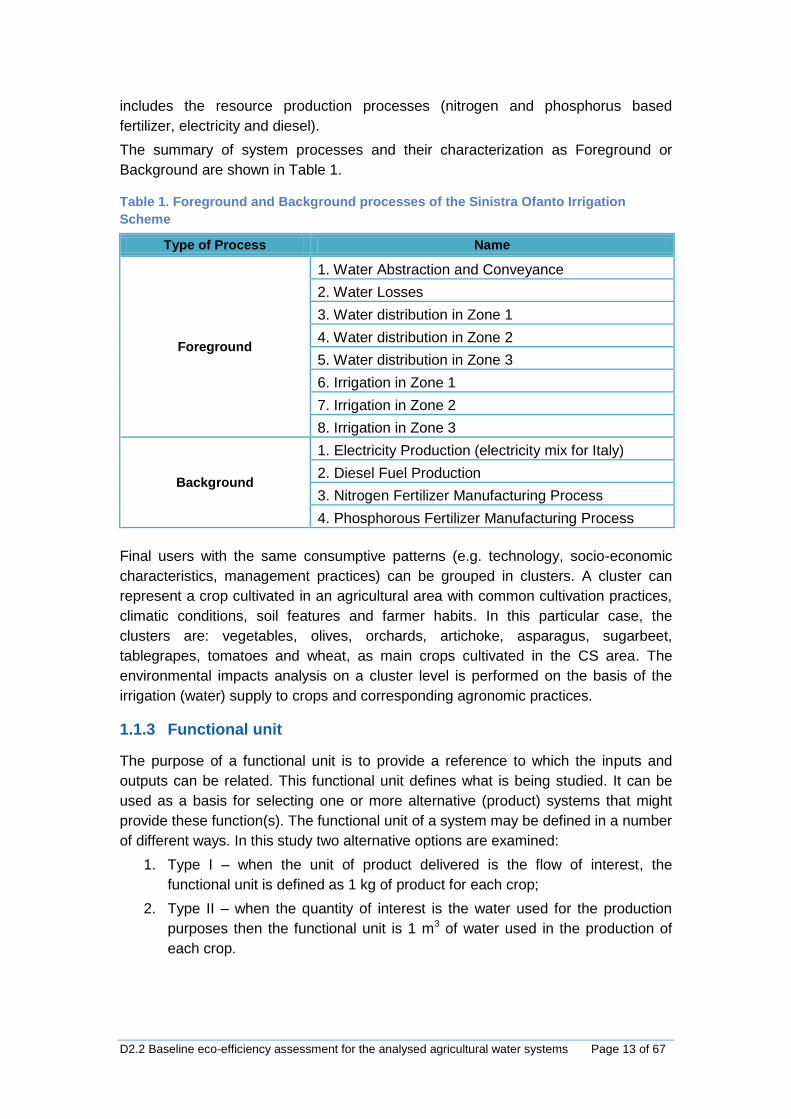
The summary of system processes and their characterization as Foreground or
Background are shown in Table 1.
Table 1. Foreground and Background processes of the Sinistra Ofanto Irrigation
Scheme
Type of Process Name
Foreground
1. Water Abstraction and Conveyance
2. Water Losses
3. Water distribution in Zone 1
4. Water distribution in Zone 2
5. Water distribution in Zone 3
6. Irrigation in Zone 1
7. Irrigation in Zone 2
8. Irrigation in Zone 3
Background
1. Electricity Production (electricity mix for Italy)
2. Diesel Fuel Production
3. Nitrogen Fertilizer Manufacturing Process
4. Phosphorous Fertilizer Manufacturing Process
Final users with the same consumptive patterns (e.g. technology, socio-economic
characteristics, management practices) can be grouped in clusters. A cluster can
represent a crop cultivated in an agricultural area with common cultivation practices,
climatic conditions, soil features and farmer habits. In this particular case, the
clusters are: vegetables, olives, orchards, artichoke, asparagus, sugarbeet,
tablegrapes, tomatoes and wheat, as main crops cultivated in the CS area. The
environmental impacts analysis on a cluster level is performed on the basis of the
irrigation (water) supply to crops and corresponding agronomic practices.
1.1.3 Functional unit
The purpose of a functional unit is to provide a reference to which the inputs and
outputs can be related. This functional unit defines what is being studied. It can be
used as a basis for selecting one or more alternative (product) systems that might
provide these function(s). The functional unit of a system may be defined in a number
of different ways. In this study two alternative options are examined:
1. Type I – when the unit of product delivered is the flow of interest, the
functional unit is defined as 1 kg of product for each crop;
2. Type II – when the quantity of interest is the water used for the production
purposes then the functional unit is 1 m3 of water used in the production of
each crop.
D2.2 Baseline eco-efficiency assessment for the analysed agricultural water systems Page 14 of 67
1.2 Inventory Analysis
Inventory analysis is used for data collection to estimate all the inputs (resources)
and outputs (emissions) in relation to the functional unit. The input and output data
include the use of resources (water, energy, fuel and N and P fertilizers) and the
releases to air, soil and water associated with the processes. Two types of data are
gathered for each unit process: environmental flows and economic flows.
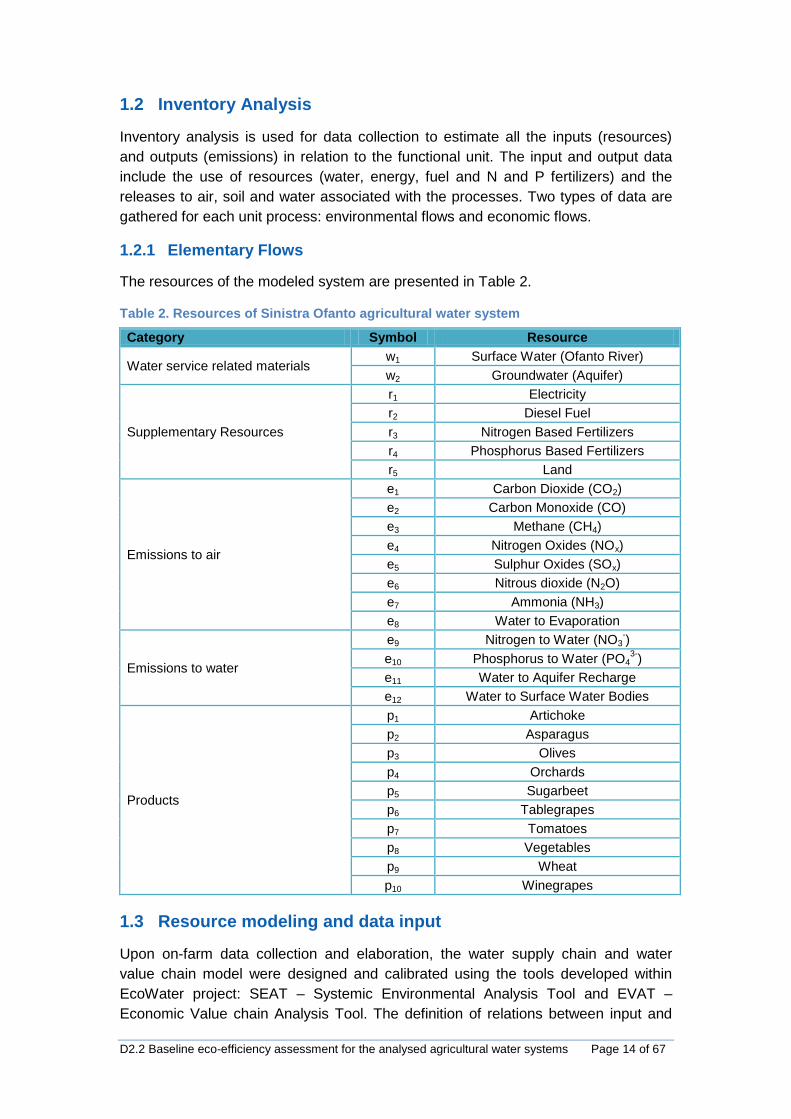
1.2.1 Elementary Flows
The resources of the modeled system are presented in Table 2.
Table 2. Resources of Sinistra Ofanto agricultural water system
Category Symbol Resource
Water service related materials w1 Surface Water (Ofanto River)
w2 Groundwater (Aquifer)
Supplementary Resources
r1 Electricity
r2 Diesel Fuel
r3 Nitrogen Based Fertilizers
r4 Phosphorus Based Fertilizers
r5 Land
Emissions to air
e1 Carbon Dioxide (CO2)
e2 Carbon Monoxide (CO)
e3 Methane (CH4)
e4 Nitrogen Oxides (NOx)
e5 Sulphur Oxides (SOx)
e6 Nitrous dioxide (N2O)
e7 Ammonia (NH3)
e8 Water to Evaporation
Emissions to water
e9 Nitrogen to Water (NO3-)
e10 Phosphorus to Water (PO43-
)
e11 Water to Aquifer Recharge
e12 Water to Surface Water Bodies
Products
p1 Artichoke
p2 Asparagus
p3 Olives
p4 Orchards
p5 Sugarbeet
p6 Tablegrapes
p7 Tomatoes
p8 Vegetables
p9 Wheat
p10 Winegrapes
1.3 Resource modeling and data input
Upon on-farm data collection and elaboration, the water supply chain and water
value chain model were designed and calibrated using the tools developed within
EcoWater project: SEAT – Systemic Environmental Analysis Tool and EVAT –
Economic Value chain Analysis Tool. The definition of relations between input and
D2.2 Baseline eco-efficiency assessment for the analysed agricultural water systems Page 15 of 67
output flows were specified along with the resource flows to and from each process
of the model of the system. The primary information supplied by CBC has been
complemented with secondary additional information, coming from scientific literature
and official statistics.
1.3.1 Water service related materials
Water abstracted from Ofanto River was estimated on the basis of total gross water
requirements (GIR) of each zone deducting water losses which were defined based
on literature review conducted for each type of distribution system. Water losses in
different stages and processes of Sinistra Ofanto irrigation scheme were modelled as
a percentage of total water flowing to stage or processes (Table 3) and are
considered as part of evaporation component of water balance.
Table 3. Water losses in different delivery stages of SO scheme
Stages – Processes Water losses (as % of total flow/volume)
Canestrello Reservoir 3%
Capaciotti Dam 7%
Canals 4%
Reservoirs 3%
Pumping station 1%
Delivery Network 2%
District Network 2%
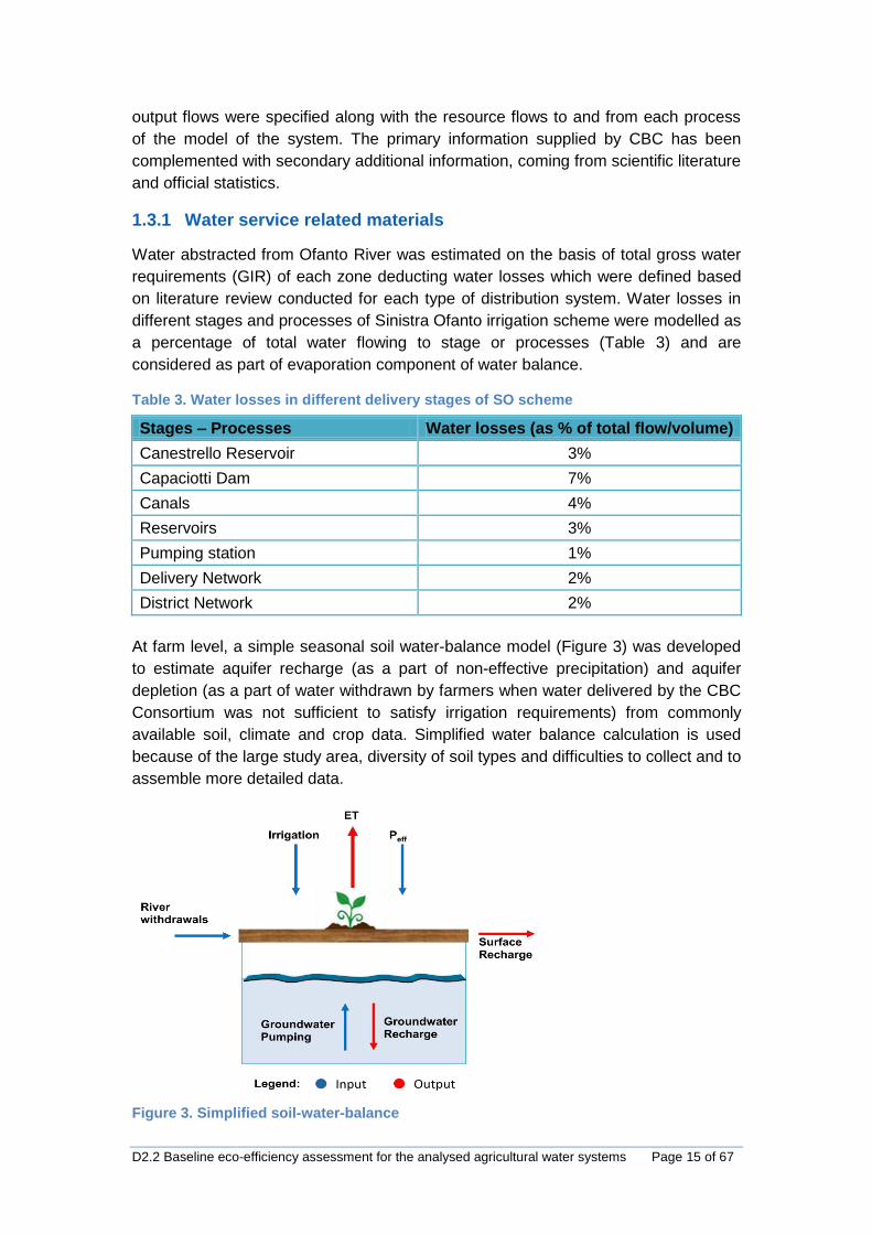
At farm level, a simple seasonal soil water-balance model (Figure 3) was developed
to estimate aquifer recharge (as a part of non-effective precipitation) and aquifer
depletion (as a part of water withdrawn by farmers when water delivered by the CBC
Consortium was not sufficient to satisfy irrigation requirements) from commonly
available soil, climate and crop data. Simplified water balance calculation is used
because of the large study area, diversity of soil types and difficulties to collect and to
assemble more detailed data.
Figure 3. Simplified soil-water-balance

D2.2 Baseline eco-efficiency assessment for the analysed agricultural water systems Page 16 of 67
The components of agricultural water balance (crop water requirements – CWR,
effective precipitation – Peff, net irrigation requirements – NIR) and crop yield
response to water were estimated for each crop on a monthly basis by using
ISAREG irrigation water management decision support tool (Pereira et al., 2003).
The Penman-Monteith reference evapotranspiration (ETo), crop evapotranpiration
(ETc) and NIR were estimated following the FAO standard method for crop
evapotranspiration estimate (Allen et al., 1998). The effective rainfall was calculated
with ISAREG over the whole growing season using the method of fixed percentage;
in this work it was fixed to 80% of total monthly precipitation. The irrigation
requirements for the baseline conditions, calculated with ISAREG model, are
presented in Table 4. These data were used to estimate the total water demand for
the three irrigation zones and the groundwater withdrawal.
Table 4. Seasonal ETc, Peff, and NIR for average and dry year conditions
Crops CWR (mm) Peff (mm) Peff_Dry (mm) NIR (mm) NIR_Dry (mm)
Artichoke 645.0 257.28 245.0 387.7 400.0
Asparagus 896.0 411.36 328.3 484.6 567.7
Olive 552.0 309.44 227.4 242.6 324.6
Orchards 714.0 227.52 133.0 486.5 581.0
Sugarbeet 677.0 314.4 269.4 362.6 407.6
Table Grape 620.0 168.96 126.6 451.0 493.4
Tomato 511.0 86.88 58.9 424.1 452.1
Vegetables 457.4 177.44 97.4 280.0 360.0
Wheat 450.8 294.88 245.8 155.9 205.0
Winegrape 524.0 168.96 126.6 355.0 397.4
The crop water demand (WDCrop) expressed as gross irrigation requirement (GIR)
was estimated for each area covered by specific crop (Acrop) according to Equation 1
from the NIR computed by ISAREG model and considering the beneficial water use
ratio (BWUR) for the network (EFFnetwork), the application efficiency of the irrigation
method (EFFmethod), and the irrigation factor W (0 for rainfed and 1 for full irrigation)
which represents the product of the percentage of area irrigated and the water supply
regime (a percentage of water supply by irrigation in respect to that necessary to
cover completely evapotranspiration demand).
c eff crop
Crop crop
method network
(ET P ) WWD A
EFF EFF
(Eq. 1)
For each zone, total water demand at the level of hydrant was expressed as a sum of
water requirements of individual crops served from that hydrant. The analysis was
conducted for different irrigation zones and for each crop in the study area (cluster).
Irrigation methods and their application efficiency are presented in Table 5. For each
method on-farm distribution efficiency of 95% was assigned to calculate overall
irrigation efficiency which is a product of irrigation method efficiency and on-farm
distribution efficiency.
D2.2 Baseline eco-efficiency assessment for the analysed agricultural water systems Page 17 of 67
Table 5. Irrigation methods in Sinistra Ofanto scheme
Method Method Efficiency, EFFmethod (%)
Farm distribution efficiency,
EFFnetwork (%)
Irrigation Efficiency,
EFFirrigation (%)
Drip(a) 0.9 0.95 0.855
Sprinkler 0.75 0.95 0.7125
Sprinkler 0.8 0.95 0.76
MicroSprinkler(b) 0.85 0.95 0.8075
Sub-Drip 0.95 0.95 0.9025
The estimation of aquifer water depletion (WAquifer) was done iteratively (from
Equations 2 and 3) based on the sum of water requirement (WD, i.e. GIR) of each
crop i (of a total of N crops) excluding water coming from the district network
(WNetwork) and water pumped from river Ofanto (WRiver) which were defined as fixed
input flows based on available data. The efficiency of water transfer from the source
to the farm was estimated as a product of efficiencies of each specific stage j (of a
total number of m stages).
nc eff crop
crop
i 1 app i
m m
j j
j 1 j 1
(ET P ) WA
EFFWDWW
EFF EFF
(Eq. 2)
aquifer network riverWW WW W W (Eq. 3)
Table 6 reports the water deliveries by the CBC recorded for 2007 which were
assumed to resemble the baseline conditions. In irrigation zones 1 and 3, farmers
abstracted from the river by booster pumps an estimated volume of 0.5 Mm3 and 1
Mm3, respectively. If necessary, the rest of water demand for all irrigation zones is
covered from the aquifer.
Table 6. Water deliveries by the CBC network for three irrigation zones in 2007 and
estimated river pumping
Water Delivered Zone 1 Zone 2 Zone 3 Total
Estimated River Pumping (m3/season) 500,000,00 0 1,000,000 1,500,000
Measured Deliveries 2007 (m3/season) 2,012,772 8,786,265 25,826,376 36,625,413
1.3.2 Supplementary Resources
1.3.2.1 Electricity and Diesel Fuel
Energy consumption is measured in kilowatt hours (kWh) based on total of volume of
water pumped throughout the irrigation season from water supply, groundwater and
river pumping. Energy requirements of all technologies (i.e. pumps, borehole drills,

D2.2 Baseline eco-efficiency assessment for the analysed agricultural water systems Page 18 of 67
hydrants, etc.) involved in the water supply chain of Sinistra Ofanto irrigation scheme
are reported in Table 7 for different irrigation zones.
Table 7. Energy requirements in the water supply chain (CBC, and pumping from river
and from aquifer)
Process/Stage Zone 1 Zone 2 Zone3
CBC Energy Requirement (kWh/m³) 0.42 0.42 0
Pumping from River Energy Requirement (kWh/m³) 0.25 0 0.25
Groundwater pumping Energy Requirement(kWh/m³) 0.35 0.35 0.35
1.3.2.2 Agrochemical requirements
Total agrochemical used for each crop was estimated per unit area of land
cultivation. Agrochemical requirement presented in Table 8 were obtained from CNR-
ISPA (Dr. Vito Cantore, pers. comm.). They represent the recommended quantity
used for plant growth and refer to pure nitrogen (N) and phosphorus (P)
requirements. Potassium (K) application is not relevant because the land in Apulia is
very reach with K and it should not be applied.
Table 8. Recommended Nitrogen and Phosphorus requirements for the crops in the CS
Crops N_Req (kg/ha/yr) P_Req (kg/ha/yr)
Artichoke 200 100
Asparagus 160 60
Olive 90 45
Orchards 110 60
Sugarbeet 110 85
Table Grape 170 95
Tomato 150 110
Vegetables 180 80
Wheat 110 33
Winegrape 170 90
1.3.2.3 Land Allocation
The crop land allocation for each irrigation zone is reported in Table 9 and refers to
the period 2007-2012.
Table 9. Crop distribution [ha] in the sub-schemes of the CS area for the baseline
Crops Zone 1 Zone 2 Zone 3
Artichoke 43 20 506
Asparagus 102 0 5
Olive 60 3656 3619
Orchards 67 13 3147
Sugarbeet 3 0 25
Table Grape 0 41 3233
Tomato 218 63 90
Vegetables 47 215 483
Wheat 2218 2604.6 1943
Winegrape 98 3793 7338
TOTAL 2856 10405 20389
D2.2 Baseline eco-efficiency assessment for the analysed agricultural water systems Page 19 of 67
1.3.3 Emissions to Air and Water
Emissions were estimated by multiplying activity data with emission factors for each
resource.
1.3.3.1 Emissions from irrigation
Pumping water for irrigation requires use of energy (electricity and/or diesel) that
could have a significant impact on the greenhouse gas (GHG) emission. The energy
requirement and emission factors from pumping water were defined for each related
resource for diesel pumps used in the on-farm water withdrawal from wells and water
pumping from the river. The resource emission factors for diesel pumps are reported
in Table 10. As a result, energy consumption and resource emissions due to water
pumping were calculated for each irrigation zone and integrated over the whole SO
irrigation scheme.
Table 10. Resource emission factor for diesel pumps used to pump water from river
and from aquifer
Resource Emission factor (kg/kWh)
CH4 0.000025
CO2 0.25
CO 0.00007
NOX 0.000007
SOX 0.0000005
The impacts from the electricity are included in the background system because
power production processes do not take place inside systems’ boundaries. Energy
requirements to pump necessary volumes of water were taken from Table 7.
Conversion from calculated diesel quantities in kWh to kg of diesel was based on
conversion factor of 11.972 (1kg of Diesel = 11.972 kWh) assuming that the Calorific
Value is 35,8 MJ/L. This conversion is required because the characterization factors
for Diesel Production were defined per kg of diesel, while in SEAT model diesel
quantities were calculated in kWh.
1.3.3.2 Emissions from the use and manufacture of farm machinery
Although a range of machines is used in cropping every year, the duration of each
operation is relatively short. On average, approximately 83.7 MJ of energy are
required to produce one kg of farm machine (Maraseni et al., 2007). Since 1 kWh =
3.6 MJ, 23.25 (83.7/3.6) kWh are required for each of those machinery kilos. About
0.70787 kg CO2eq are emitted for each kWh of electricity production. Hence, for
producing each kg of machinery 16.45 kg (0.70787 x 23.25) of CO2eq GHGs are
emitted into the atmosphere. Based on the work of Maraseni et al. (2007), the
following equation was used to estimate tractor-generated GHG emissions:
Machinery GHGs emission (kgCO2eq/ha) = Weight of machine (kg) x 16.45 kgCO2eq
kg-1 x Fraction of lifespan of that machine used for a ha of that land use (Eq. 4)
Average operation hour for farm operations and machine power used are reported in
Table 11. Those data, provided by CNR-ISPA, are verified and adjusted by the
relevant landholders in the CS area. Farm Operations include Plowing, Fertilization,
D2.2 Baseline eco-efficiency assessment for the analysed agricultural water systems Page 20 of 67
Weed control, Chemical Treatments, Trans-plantation and Harvesting. Harvesting is
given separately as for this operation for certain crop is used a different machine.
Average weight of machines and average working life were assumed to be 8,000kg
and 10,000 hour, respectively.
Table 11. Average Operation hours and machine power for different farm operations
(CBC, CNR-ISPA)
Crops Working
hours
Working hours (Only
for Harvesting)
Total Working
hours
Machine Power (kW)
Machine Power for Harvesting
(kW)
Artichoke 10.5 16 26.5 80 45
Asparagus 9.5 16 25.5 80 30
Olive 12 2 14 80 -
Orchards 15 2 17 60 -
Sugarbeet 8 3 11 80 130
Table Grape 19.5 8 27.5 45 -
Tomato 13 3 16 80 -
Vegetables 10.5 3 13.5 80 -
Wheat 5 1 6 80 130
Winegrape 17.5 8 25.5 45 -
1.3.3.3 Emissions from fuel use in farm operations
The total fuel consumption and GHG emissions for each liter (L) of fuel was used to
calculate the total amount of GHG emissions from fossil fuel usage. GHG emissions
from fuel use in farm machinery were calculated as follows:
Fuel GHGs (kgCO2eq/ha) = Fuel (L/ha) • Emission Factor (kgCO2eq/L) (Eq. 5)
Fuel consumption was derived from working hours and power of machine (fuel
consumption = Power of machine in kW·0.25 L hour-1 kW-1·hour used) (Smith, 2004).
Each litre of diesel produces 2.66 kg CO2eq during its combustion. Combustion of
fossil fuel also emits methane (CH4) and nitrous oxide (N2O). Each litre of diesel
combustion gives of 2.66 kg CO2, 0.000383 kg methane (0.009575 kg CO2eq) and
0.0007645 kg nitrous oxide (0.2278 kg CO2eq) (Nussey, 2005). Therefore, the total
greenhouse gases emissions during combustion of one litre of diesel is 2.837
kgCO2eq L-1 (2.66 + 0.009575 + 0.2278 = 2.8974 kgCO2 L
-1).
1.3.3.4 Emissions from fertilizer use
In addition to the GHG emissions associated with the manufacturing and
acquirement of N and P fertilizers, the application of N and P results in emission into
air, soil and water. With respect to agricultural soils, the emissions can be classified
as direct or indirect. Direct emissions are linked to direct nitrogen additions to the
agricultural soils like nitrogen fertilizer and animal manure, nitrogen fixation, crop
residues and cultivation of histosols. Indirect emissions are the result of the
subsequent leaching of nitrate from agricultural soils to ground water and surface
waters and ammonia (NH3) volatilization. Scientific background of direct and indirect

D2.2 Baseline eco-efficiency assessment for the analysed agricultural water systems Page 21 of 67
N2O emissions from agricultural soils is explained elsewhere (Eggleston, 2006; van
Schijndel 2007). In order to provide a useful approximation of GHG emissions from
direct (nitrification and denitrification) and indirect (leaching, runoff, and ammonia
(NH3) volatilization) soil emission from N application and P emissions we used a
simplified concept as presented in Figure 4.
Figure 4. Simplified concept of N and P balances
The IPCC default values for emission factors were used in this study in combination
with the CS activity data on fertilizer application for each crop as presented
previously in Table 8. Low, average, and high emission factors for estimating N2O
emissions from N fertilizer and lime are proposed by the IPCC guidelines (Eggleston
et al., 2006) as presented in Table 12.
Table 12. Low, average, and high emission factors used for estimating N2O emissions
from N fertilizer and lime using IPCC (Eggleston et al., 2006) guidelines.
Low Average High
Emission factor for direct N2O emission 0.003 0.01 0.03
Fraction of N fertilizier that volatilizes 0.05 0.2 0.5
Emission factor for volatilized N 0.002 0.01 0.05
Fraction of N fertilizier that leach 0.1 0.3 0.8
Emission factor for leached N 0.0005 0.0075 0.025
Emission factor for applied lime 0.12 0.125 0.13
Direct emissions are computed as the product of the direct N2O emissions factor and
the amount of N applied. The global mean fertilizer-induced emissions for N2O and
NO amount to 0.9% and 0.7%, respectively, of the N applied (Bouwman, 2002).
However, due to the uncertainties associated with N2O and the inclusion in the
inventory calculation of other contributions to the nitrogen additions (e.g., from crop

D2.2 Baseline eco-efficiency assessment for the analysed agricultural water systems Page 22 of 67
residues and the mineralisation of soil organic matter), the round value of 1% is
appropriate (Eggleston, 2006). This method estimates the total direct N2O emissions,
irrespective of type of soils, of land use (e.g. grassland and cropland soils) and of
vegetation, irrespective of the nitrogen compounds (e.g. organic, inorganic nitrogen),
and irrespective of climatic factors.
Indirect N2O emissions were broken down into those due to volatilization and those
due to leaching or runoff. Each indirect emission path is calculated as the product of
the amount of N applied, the fraction of N lost through that emission path, and the
emission factor for that path. Leaching in groundwater and surface runoff fractions
are expressed in percentage of N and P applied via fertilizer and calculated from the
amount of applied fertilizers. The IPCC default value for fraction of N lost in leaching
and runoff is 30%. For humid regions or in dryland regions where irrigation (other
than drip irrigation) is used, the default FracLEACH-(H) is 0.30. For dry land regions,
where precipitation is lower than evapotranspiration throughout most of the year and
leaching is unlikely to occur, the default FracLEACH is zero. In Sinistra Ofanto, the
command area is a flat plain and soil is mainly loamy clay with low percolation
potential. Taking into account the slope of the area, precipitation surplus, irrigation,
evaporation, soil type and diversity of crops grown, N leached for Sinistra Ofanto
area was assumed 20% of N fertilizer applied and partitioned as 10% into
groundwater and 10% into surface water. It is assumed that all N that leaches from
the rooting zone is present as NO3-. Beyond the original site of N additions, the
indirect N2O emissions occur from N leached/lost in runoff with an emission factor of
0.75% of N leached (Eggleston, 2006).
The losses through NH3-N volatilization were based on IPCC methodology which
assumes that 10% of the fertilizer applied is lost through NH3-N volatilization. The
IPCC Guidelines explain that the calculations should be based on the emissions of
NOx and NH3 originating from nitrogen fertilizers and animal manure in the country
and not on the deposition of NOx and NH3 on the country territory. Atmospheric
deposition of nitrogen was calculated using the IPCC default emission factor 0.01 kg
N2O-N per kg emitted NH3.
Conversion of emission for each pollutant (N2O, NH3, NO3) was performed by
dividing the molecular/ionic mass of the species with the atomic mass of N.
Conversion between emission gases was made according to the standard suggested
by the IPCC (Eggleston et al., 2006).
The partitioning of P was assumed as 3% to surface water, 2% to groundwater and
4% for immobilization into calcium phosphate which cannot be used by plants (pers.
comm. Judgment, Dr. Vito Cantore, CNR-ISPA). It is assumed that all P that leaches
is present as PO43-. Conversion factor 3.06 is used to convert from PO4
3-- P to PO43-.
1.3.4 Water to Aquifer Recharge, Surface Recharge and Evaporation
The difference between total annual precipitation and effective rainfall for each
crop was assumed to be partitioned into the recharge of surface and groundwater
and evaporation losses by 30, 30, and 40 %, respectively.
D2.2 Baseline eco-efficiency assessment for the analysed agricultural water systems Page 23 of 67
1.3.5 Products
After model validation on the data from the farms, the crop yield vs water input
polynomial relationship was generated running the ISAREG model for different
irrigation scheduling options (from full to rainfed). The model validation was
performed on the statistical data collected in the CS area for 2007. The polynomial
relationship was used in SEAT to estimate total agricultural production expressed as
crop yield per area of land cultivation. These data are obtained from the simulations
of crop yield under different irrigation input in ISAREG model and the results for each
crop are shown in Table 13 for normal and dry hydrological year.
Table 13. Crop yield (CY) vs irrigation water factor (W) input as a polynomial
relationship CY=A•W2+B•W+C
Condition NORMAL YEAR DRY YEAR
Crops A B C A B C R²
Artichoke -0.37 0.9093 0.4813 -0.11 0.667 0.4515 0.98
Asparagus -0.0387 0.4145 0.6379 0.0002 0.466 0.5302 0.98
Olive 0.0046 0.2254 0.7558 -0.1 0.469 0.6257 0.99
Orchards -0.0081 0.5787 0.4309 -0.14 0.8787 0.2802 0.99
Sugarbeet -0.2086 0.596 0.6264 0.0036 0.496 0.5025 0.98
Table Grape -0.0954 0.5614 0.5266 -0.03 0.572 0.4738 0.99
Tomato 0.2529 0.3792 0.3843 -0.02 0.8076 0.2228 0.99
Vegetables -0.1517 0.667 0.5064 -0.47 1.18 0.31 0.98
Wheat -0.1257 0.2938 0.8368 0.0519 0.267 0.6919 0.98
Winegrape -0.096 0.5485 0.5602 -0.19 0.673 0.5297 0.99
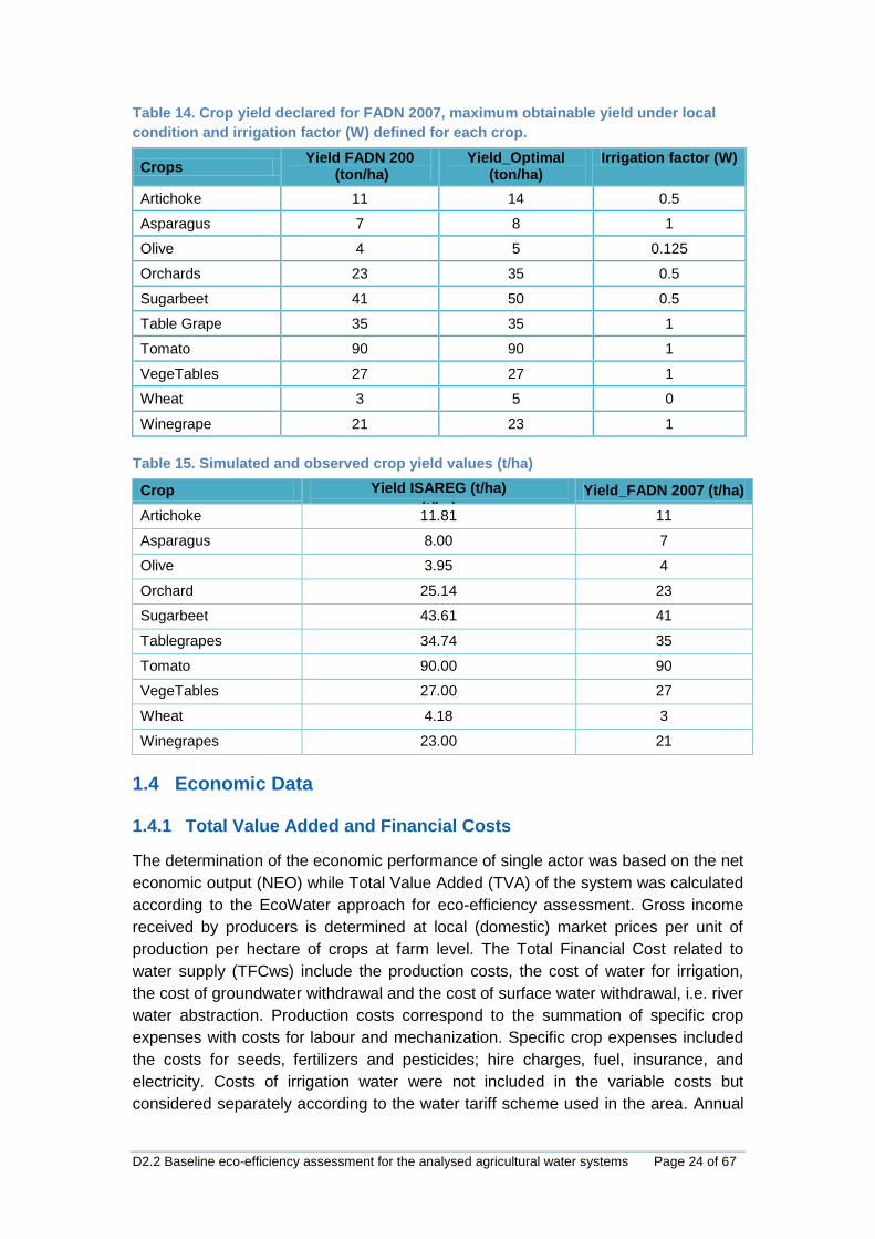
Eventual relative crop yield reduction was linked to the irrigation factor W assigned to
each crop referring full or deficit irrigation supply. Irrigation factor is defined for each
crop after comparing the data declared by farmers and obtained from FADN (Farm
Accountancy Data Network) database and crop maximum yield under local
conditions. After comparing the data and discussing with local stakeholders we
concluded that artichoke, orchards and sugarbeet were irrigated at 50% of water
requirements and olives at 50% of water requirements over 50% of cultivated area
while the rest was kept under rainfed. All other crops were under full irrigation regime
while wheat was cultivated completely in rainfed. Relative yield is calculated
proportionally to the maximum obtainable yield and irrigation factor, both estimated
for the CS area and reported in Table 14.
Crop yield values were estimated by ISAREG model and the results of simulations
were compared with the data available in the literature and in the practice (on-farm
investigation in the case study area). The results of comparison for the most
important crops grown in the Sinistra Ofanto are reported in Table 15. A good
agreement was observed between the simulated data and those coming from the
literature/case study area.
D2.2 Baseline eco-efficiency assessment for the analysed agricultural water systems Page 24 of 67
Table 14. Crop yield declared for FADN 2007, maximum obtainable yield under local
condition and irrigation factor (W) defined for each crop.
Crops Yield FADN 200
(ton/ha) Yield_Optimal
(ton/ha) Irrigation factor (W)
Artichoke 11 14 0.5
Asparagus 7 8 1
Olive 4 5 0.125
Orchards 23 35 0.5
Sugarbeet 41 50 0.5
Table Grape 35 35 1
Tomato 90 90 1
VegeTables 27 27 1
Wheat 3 5 0
Winegrape 21 23 1
Table 15. Simulated and observed crop yield values (t/ha)
Crop Yield ISAREG (t/ha)
(t/ha) Yield_FADN 2007 (t/ha)
Artichoke 11.81 11
Asparagus 8.00 7
Olive 3.95 4
Orchard 25.14 23
Sugarbeet 43.61 41
Tablegrapes 34.74 35
Tomato 90.00 90
VegeTables 27.00 27
Wheat 4.18 3
Winegrapes 23.00 21
1.4 Economic Data
1.4.1 Total Value Added and Financial Costs
The determination of the economic performance of single actor was based on the net
economic output (NEO) while Total Value Added (TVA) of the system was calculated
according to the EcoWater approach for eco-efficiency assessment. Gross income
received by producers is determined at local (domestic) market prices per unit of
production per hectare of crops at farm level. The Total Financial Cost related to
water supply (TFCws) include the production costs, the cost of water for irrigation,
the cost of groundwater withdrawal and the cost of surface water withdrawal, i.e. river
water abstraction. Production costs correspond to the summation of specific crop
expenses with costs for labour and mechanization. Specific crop expenses included
the costs for seeds, fertilizers and pesticides; hire charges, fuel, insurance, and
electricity. Costs of irrigation water were not included in the variable costs but
considered separately according to the water tariff scheme used in the area. Annual

D2.2 Baseline eco-efficiency assessment for the analysed agricultural water systems Page 25 of 67
price and production cost including variable and fixed costs (Table 16) were obtained
from regional economic data Farm Accountancy Data Network (FADN, 2007).
Table 16. Gross Market Price and production cost (FADN, 2007)
Crops Price (€/t) Production Cost (€/ha)
Artichoke 736 5795
Asparagus 1142 5052
Olive 1297 2932
Orchards 516 5074
Sugarbeet 53 1950
Tablegrapes 423 6556
Tomato 95 4702
VegeTables 408 3513
Wheat 341 548
Winegrapes 258 4424
1.4.2 Water tariffs
In the case of the “Sinistra Ofanto” irrigation scheme farmers usually pay for irrigation
service a tariff that is composed of two parts, a fixed rate with a fixed annual tariff per
hectare (15.5 €/ha), which must be paid whether irrigated or not to cover running
costs, and a variable rate which depends on volume of water used with an average
water duty 2050 m3/ha and with three levels as indicated hereafter:
0.09 €/m3 for seasonal water withdrawal between 0 - 2050 m3/ha;
0.18 €/m3 for seasonal water withdrawal between 2050 - 3000 m3/ha;
0.24 €/m3 for seasonal water withdrawals higher than 3000 m3/ha.
The water fees include all the costs of personnel, maintenance of structures, and
consumables, but they do not include any profit mark-up, because the CBC is a non-
profit organization and operates under the regime of full cost-sharing among the
water users. In reality, the CBC bears the cost of 0.2 €/m3 for supplying water in zone
1, 0.19 €/m3 for supplying water in zone 2 and 0.16 €/m3 for supplying water in zone
3. Although the cost for supplying irrigation water is significantly different between the
areas supplied by gravity and those served by pumping and/or lifting, the CBC
applies the same irrigation tariffs regardless the location of farms. In such a way, the
CBC has enforced the principle of solidarity among the farmers and different served
areas (irrigation zones 1, 2 and 3). Referring to other sources of water, farmers bear
the cost of 0.40 €/m3 (which includes equipment costs and energy costs) for
groundwater abstraction and 0.20 €/m3 for pumping water directly from Ofanto River.
1.5 Baseline eco-efficiency assessment
1.5.1 Calculated life cycle inventory flows (Normal Hydrological Year)
Calculation of life cycle inventory flow for baseline conditions was performed for
normal and dry year, corresponding to annual precipitation of 514 (similar to year
D2.2 Baseline eco-efficiency assessment for the analysed agricultural water systems Page 26 of 67
2007) and 420 mm (similar to year 1990), respectively. The baseline scenario refers
to the management practices in 2007, i.e. the application of deficit irrigation strategy
for artichoke, olives, orchards and sugarbeet, when other crops were cultivated under
full irrigation while wheat was under rainfed conditions as described previously. The
year 2007 was assumed to be the most appropriate for the baseline eco-efficiency
assessment because of data availability related to water distribution, crops cultivation
and market prices etc. Moreover, the precipitation in that year was very close to the
22-years average precipitation (1990-2011). Finally, the local stakeholders (CBC)
indicated that year as the most appropriate one because some changes in the water
management and the introduction of new technologies and management practices
started since that period. Accordingly, the water supply and value chain mapping
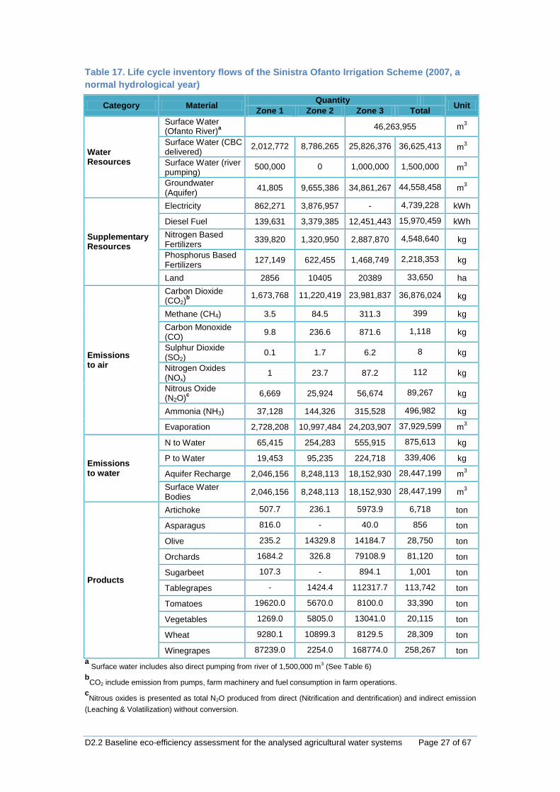
were performed for the baseline conditions in SEAT and EVAT. Table 17 presents
the calculated life cycle inventory flows for each irrigation zone for normal conditions.
This information for the use of resources was extracted from SEAT model and all
flows are referred to annual average values.
Total water withdrawal from Ofanto river was estimated by SEAT to be approximately
44,7 Mm3 taking into account the on-farm water availability of 36.6 Mm3 and water
conveyance, delivery and storage losses as described in section 1.3.1. Water
delivery simulated by SEAT fits well the volumes effectively delivered by the CBC in
2007. Overall losses in conveyance, storage and distribution account are about 8.1
Mm3 or 18 % of total volume withdrawn. This is also in accordance with the values
provided by the CBC where losses ranged from 15-20%. According to our model the
highest losses occurred in canal due to the highest volume conveyed and relatively
high conveyance distance. The assessment of global water losses shows that
system performs good. Total water use on farm level, including the groundwater
withdrawal and surface water originated from Ofanto River was estimated as 82.6
Mm³ showing that the groundwater accounts in on-farm water input for 54%. There
was significant difference among groundwater use between irrigation zones
indicating that groundwater pumping was mostly affected by different cropping
patterns and water management practices. Zone 1 presents the lowest groundwater
withdrawals due to high presence of wheat (78%) which is not irrigated. In zone 2,
with a diversified cropping pattern, more than 50% of total water requirements were
fulfilled from aquifer. The highest groundwater withdrawals were found in zone 3 with
a rate of 1889 m3/ha due to largest surface area and high allocation of water
demanding crops. Similar results for groundwater exploitation varying between 1000
and 4000 m3/ha were simulated by Oueslati (2007) in Sinistra Bradano scheme
located close to the Sinistra Ofanto irrigation scheme. The water recharge mostly
occurs during the autumn and winter months. The total annual recharge of
groundwater and surface water from average precipitation of 514 mm/year is
estimated as 56.8 Mm3 which represents about 63% of total water withdrawal and
corresponds to overall water deficit of 34 Mm3. The annual recharge of the aquifer
was estimated as 28.45 Mm3 which, in the case of average year, represents about
64% of water withdrawal from the aquifer and indicates an annual trend of water
depletion in the aquifer of 16.11 Mm3.
D2.2 Baseline eco-efficiency assessment for the analysed agricultural water systems Page 27 of 67
Table 17. Life cycle inventory flows of the Sinistra Ofanto Irrigation Scheme (2007, a
normal hydrological year)
Category Material Quantity
Unit Zone 1 Zone 2 Zone 3 Total
Water Resources
Surface Water (Ofanto River)
a
46,263,955 m3
Surface Water (CBC delivered)
2,012,772 8,786,265 25,826,376 36,625,413 m3
Surface Water (river pumping)
500,000 0 1,000,000 1,500,000 m3
Groundwater (Aquifer)
41,805 9,655,386 34,861,267 44,558,458 m3
Supplementary Resources
Electricity 862,271 3,876,957 - 4,739,228 kWh
Diesel Fuel 139,631 3,379,385 12,451,443 15,970,459 kWh
Nitrogen Based Fertilizers
339,820 1,320,950 2,887,870 4,548,640 kg
Phosphorus Based Fertilizers
127,149 622,455 1,468,749 2,218,353 kg
Land 2856 10405 20389 33,650 ha
Emissions to air
Carbon Dioxide (CO2)
b
1,673,768 11,220,419 23,981,837 36,876,024 kg
Methane (CH4) 3.5 84.5 311.3 399 kg
Carbon Monoxide (CO)
9.8 236.6 871.6 1,118 kg
Sulphur Dioxide (SO2)
0.1 1.7 6.2 8 kg
Nitrogen Oxides (NOx)
1 23.7 87.2 112 kg
Nitrous Oxide (N2O)
c
6,669 25,924 56,674 89,267 kg
Ammonia (NH3) 37,128 144,326 315,528 496,982 kg
Evaporation 2,728,208 10,997,484 24,203,907 37,929,599 m3
Emissions to water
N to Water 65,415 254,283 555,915 875,613 kg
P to Water 19,453 95,235 224,718 339,406 kg
Aquifer Recharge 2,046,156 8,248,113 18,152,930 28,447,199 m3
Surface Water Bodies
2,046,156 8,248,113 18,152,930 28,447,199 m3
Products
Artichoke 507.7 236.1 5973.9 6,718 ton
Asparagus 816.0 - 40.0 856 ton
Olive 235.2 14329.8 14184.7 28,750 ton
Orchards 1684.2 326.8 79108.9 81,120 ton
Sugarbeet 107.3 - 894.1 1,001 ton
Tablegrapes - 1424.4 112317.7 113,742 ton
Tomatoes 19620.0 5670.0 8100.0 33,390 ton
Vegetables 1269.0 5805.0 13041.0 20,115 ton
Wheat 9280.1 10899.3 8129.5 28,309 ton
Winegrapes 87239.0 2254.0 168774.0 258,267 ton
a Surface water includes also direct pumping from river of 1,500,000 m
3 (See Table 6)
bCO2 include emission from pumps, farm machinery and fuel consumption in farm operations.
cNitrous oxides is presented as total N2O produced from direct (Nitrification and dentrification) and indirect emission
(Leaching & Volatilization) without conversion.

D2.2 Baseline eco-efficiency assessment for the analysed agricultural water systems Page 28 of 67
Energy use varies considerably between three irrigation zones depending largely on
water supply. Although water is delivered and distributed to the farmers by gravity,
zone 3 is the major contributor to the energy consumption and related resource
emissions due to the greatest groundwater pumping to the fields. Total GHG
emissions from the use of pumps for irrigation were estimated at 119 kg CO2eq ha-1.
Insignificant emissions resulted for CH4, CO, NOx and SOx which accounted for only
0.041% of total CO2eq emission.
The main source of field losses for N was ammonia (NH3) volatilization. Ammonia is
not a GHG, but some of this N in the atmosphere can return to the soil through
atmospheric deposition, of which a certain amount will be nitrified, denitrified, or lost
as N2O. Nitrous oxide (N2O) was the main source for field emissions. The total direct
nitrous oxide emissions (N2O) from agricultural soils for Sinistra Ofanto were
estimated at 89.2·103 kg or 26.6·106 kgCO2eq. This corresponds with 2.62 kgN2O·ha-1
or 795 kg CO2eq·ha-1 agricultural soil. The largest source of N2O was emitted through
nitrification and denitrification which accounted for 80% of total N2O emissions.
Indirect emissions accounted for 12% in leaching and runoff and 8% from
volatilization. The distribution of these emissions through different pathways is shown
in Figure 5. The total GHG emissions from operation of machinery and fuel
consumption ranged from 207 kg CO2-eq ha-1 to 770 kg CO2-eq ha-1. In consistence
with Table 11, the highest source for this emission was artichoke cultivation due to
high working hours and high power of machine needed for farm operations.
Figure 5. Greenhouse gas emissions from farm supplementary resources in Sinistra Ofanto irrigation scheme
Total agricultural production amounts to 572·103 ton with the highest production of
winegrapes of about 45% of total production due to highest land allocation and
relatively high production yield.
21,3
3,2
2,1
25,36
4,97 6,98
-
5,0
10,0
15,0
20,0
25,0
30,0
GHG Fertilizier GHG FuelConsumption
GHG Irrigation GHG Machinery
Millio
ns k
g C
O2eq
GHG Direct GHG Leaching GHG Volatilization
GHG Fuel Consumption GHG Irrigation GHG Machinery
D2.2 Baseline eco-efficiency assessment for the analysed agricultural water systems Page 29 of 67
1.5.2 Calculated life cycle inventory flows (Dry Year)
Table 18 presents the calculated life cycle inventory flows for each irrigation zone for
dry year conditions with a precipitation of about 420 mm/year and effective
precipitation and crop irrigation water requirements presented in Table 4. Total water
requirements were increased by approximately 11 Mm3 or 12% comparing to a
normal hydrological year. This increase in water requirements was compensated by
the groundwater withdrawals which reached 55.5 Mm3. The overall water deficit has
increased from 34 Mm3 (for a normal hydrological year) to 52.2 Mm3. The highest
water requirements and groundwater withdrawal are observed in irrigation zone 3
mainly due to intensive cultivation of vineyards which in zone 3 constitute 52% of
total cultivated area. Due to increase of groundwater withdrawals energy
consumption was increased in respect to normal hydrological year by 24% which
means 24% higher related resource emissions in the atmosphere. No changes in
emission from fertilizer, farm operation and machinery occurred due to no change in
fertilizer application and on farm management practices. Overall total agricultural
production decreased by 2.1% mostly affected from wheat with total decrease of 17%
for three irrigation zones.
D2.2 Baseline eco-efficiency assessment for the analysed agricultural water systems Page 30 of 67
Table 18. Life cycle inventory flows of the Sinistra Ofanto Irrigation Scheme (Dry Year)
Category Material Quantity
Total Unit Zone 1 Zone2 Zone 3
Water Resources
Surface Water (Ofanto River)
a
46,263,955 m3
Surface Water (CBC delivered)
2,012,772 8,786,265 25,826,376 36,625,413 m3
Surface Water (river pumping)
500,000 0 1,000,000 1,500,000 m3
Groundwater (Aquifer)
355,864 12,252,337 42,936,711 55,544,912 m3
Supplementary Resources
Electricity 862,271 3,876,957 - 4,739,228 kWh
Diesel Fuel 249,552 4,288,318 15,277,849 19,815,719 kWh
Nitrogen Based Fertilizers
339,820 1,320,950 2,887,870 4,548,640 kg
Phosphorus Based Fertilizers
127,149 622,455 1,468,749 2,218,353 kg
Land 2,856 10,405 20,389 33,650 ha
Emissions to air
Carbon Dioxide (CO2)
b
1,701,272 11,448,207 24,690,186 37,839,665 kg
Methane (CH4) 6 107 382 495 kg
Carbon Monoxide (CO)
17 300 1,069 1,386 kg
Sulphur Dioxide 0 2 8 10 kg
Nitrogen Oxides (NOx)
2 30 107 139 kg
Nitrous Oxide (N2O)c 6,669 25,924 56,674 89,267 kg
Ammonia (NH3) 37,128 144,326 315,528 496,982 kg
Evaporation 2,229,414 9,531,190 21,287,410 33,048,014 m3
Emissions to water
N to Water 65,415 254,283 555,915 875,613 kg
P to Water 19,453 95,235 224,718 339,406 kg
Aquifer Recharge 1,672,061 7,148,393 15,965,557 24,786,011 m3
Surface Water Bodies
1,672,061 7,148,393 15,965,557 24,786,011 m3
Products
Artichoke 456 212 5,365 6,033 ton
Asparagus 813 - 39.86 853 ton
Olive 205 12,481 12,355 25,041 ton
Orchards 1,607 312 75,488 77,407 ton
Sugarbeet 92 - 770 862 ton
Tablegrapes - 1,435 113,155 114,590 ton
Tomatoes 19,620 5,670 8,100 33,390 ton
Vegetables 1,269 5,805 13,041 20,115 ton
Wheat 7,673 9,012 6,722 23,407 ton
Winegrapes 87,239 2,254 168,774 258,267 ton
a Surface water includes also direct pumping from river of 1,500,000 m
3 (See Table 6)
bCO2 include emission from pumps, farm machinery and fuel consumption in farm operations.
cNitrous oxides is presented as total N2O produced from direct (Nitrification and dentrification) and indirect emission
(Leaching & Volatilization) without conversion.
D2.2 Baseline eco-efficiency assessment for the analysed agricultural water systems Page 31 of 67
1.5.3 Environmental Impact Assessment of the Entire System
Based on the list of the midpoint impact indicators proposed in the approach followed
by the EcoWater Project (EcoWater, 2013), 11 impact categories were selected as
the more representative for the environmental assessment of the system. Indicators
considered, related units and the characterization factors which were used for the
estimation of the impact of the foreground systems and the environmental impact
factors for the background process are presented in Tables 19 and 20, respectively.
The environmental impact factors are obtained from open access databases.
Table 19.Characterization Factors of foreground elementary flows (CML, 2001, Milà i
Canals, et al., 2009).
Impact Category
Unit N to
Water (per kg)
P to Water
(per kg)
CO2
(per
kg)
CH4
(per
kg)
N₂O
(per
kg)
CO
(per kg) SO2
(per kg)
NOX
(per
kg)
NH₃
(per
kg)
Climate Change kg CO2,eq - - 1 25 298 - - -
Eutrophication kg PO4-3
,eq 0.1 1 - - - - - 0.13
Acidification kg SO2-,eq - - - - - - 1.2 0.5 1.88
Human Toxicity kg 1,4-DCB,eq - - - - - - 0.096 1.2
Respiratory Inorganics
kg PM2.5,eq - - - - - - - -
Aquatic Ecotoxicity
kg 1,4-DCB,eq - - - - - - - -
Terrestrial Ecotoxicity
kg 1,4-DCB,eq - - - - - - - -
Photochemical Ozone Formation
kg C2H4,eq - - - 0.01 - 0.027 0.048 0.03
Minerals Depletion
kg Fe,eq - - - - - - - - -
Fossil Fuels Depletion
kg oil,eq - - - - - - - - -
Table 20. Environmental Impact Factors for Background Processes
Impact Category
Unit Electricity Production (per kWh)
Diesel Production
(per kg)
Nitrogen Fertilizer
Production (per kg)
Phosphorus Fertilizer
Production (per kg)
Climate Change kg CO2,eq 0.70787 0.38199 1.93006 0.39097
Eutrophication kg PO4-3
,eq 0.00017 0.00018 0.00035 0.06724
Acidification kg SO2-,eq 0.00407 0.00257 0.02339 0.02197
Human Toxicity kg 1,4-DCB,eq 0.09159 0.03782 0.64951 0.16316
Respiratory
Inorganics kg PM2.5,eq 0.00059 0.00035 0.00314 0.00300
Freshwater
Aquatic
Ecotoxicity
kg 1,4-DCB,eq 0.00184 0.00296 0.22896 0.08853
Terrestrial
Ecotoxicity kg 1,4-DCB,eq 0.00090 0.00101 0.00022 0.00063
Photochemical
Ozone
Formation
kg C2H4,eq 0.00018 0.00023 0.00100 0.00093
Minerals
Depletion kg Fe,eq 0.00019 0.00084 0.00000 0.00000
Fossil Fuels
Depletion kg oil,eq 0.06034 1.19438 0.97804 0.14833
•Data for electricity production and diesel production are obtained from ELCD database (ELCD, 2013) and for fertilizer production from USLCI database (USLCI, 2013)

D2.2 Baseline eco-efficiency assessment for the analysed agricultural water systems Page 32 of 67
1.5.3.1 Environmental Impact Assessment of the Entire System (Normal
Hydrological Year)
The results of the environmental impacts of the entire system including also the
results of the environmental impacts Type I (environmental impacts per unit of
product – kg of yield) and Type II Impact Indicators (environmental impacts per m3 of
water used) for average climatic conditions are presented in Table 21.
Disaggregation on the clusters level for a normal hydrological year is shown in Annex
A. The contribution of background and foreground system in the environmental
impact assessment is given in Figure 6 while the environmental impact breakdown
for each indicator is presented in Figures 7 and 8. The studied system is
characterized by significant contribution of the foreground processes in climate
change impact category due to direct emissions from fertilizer consumption,
eutrophication of groundwater and surface water due to NO3 and PO43- leaching,
acidification on non-agricultural soils through deposition of NH3 and freshwater
depletion due to irrigation (Figure 6).
Comparing the performance of the different clusters (i.e. crops), it is observed that, in
type I of indicator (based on crop production) olives, asparagus and wheat had the
highest impact indicators in most cases. The highest impacts refer to olives which
represent higher unitary emission in respect to wheat and lower emission in respect
to asparagus. However, when the environmental impacts are divided by the yield
production, then the highest environmental impacts indicator corresponds to olives
which has the lowest yield value (3.92 ton/ha). For olives, the most relevant impact
categories in foreground processes are climate change and eutrophication potential
whereas in background processes it is eutrophication potential. Wheat crop has the
highest contribution in foreground processes related to acidification and in
background processes to the freshwater aquatic eco-toxicity. On one side, this is due
to greater induced related unitary emission of wheat in respect to olives and the
lower in respect to asparagus. On the other hand, this is due to the fact that wheat
has lower yield than asparagus but higher than olives. Asparagus presents the
highest impact indicators in the case of foreground processes for impact categories
of freshwater depletion, human toxicity and in the case of background processes for
impact categories of human toxicity, respiratory inorganics, terrestrial eco-toxicity,
photochemical ozone formation, mineral depletion, fossil depletion. This is because
asparagus has the unitary highest related emission due to the highest water
requirements, leading to a higher impact on the environment, directly associated with
the water depletion, and also with the energy consumption (used in the water
distribution process) and the corresponding impacts, among other factors.
From graphs of Type II indicators (given in Annex A and based on water use) the
olives, characterized by the lowest unitary related emission and unitary water use,
lead to highest impact indicator. This is explained by the fact that Type II indicators
represent the ratio between the environmental impacts and crop water use. Hence,
the crops with the high irrigation requirements are those with the lowest impact
indicators. The exception is for the mineral depletion and terrestrial eco-toxicity
impact categories where the highest impact refers to asparagus which for this
category has the highest unitary related emission. The same is true for impact

D2.2 Baseline eco-efficiency assessment for the analysed agricultural water systems Page 33 of 67
indicator of human toxicity for foreground processes where the highest impact is
caused by tablegrapes.
Table 21. Environmental Impacts of the Study System (Normal Hydrological Year)
Indicator Value (Unit)
Foreground Value (Unit)
Background Value(Unit)
Type I Indicator (per kg
product)
Type II Indicator (per m
3
water used)
Climate Change (tCO2eq)
76,988,401 63,477,607 13,510,794 0.1345 0.9311
Fossil Fuels Depletion (kg oil,eq)
6,657,080 0 6,657,080 0.0116 0.0805
Freshwater Resource Depletion (m
3)
13,623,492 13,623,492 0 0.0238 0.1648
Eutrophication (kgPO4eq)
878,982 727,182 151,800 0.0015 0.0106
Human Toxicity (kg1,4-DBeq)
3,800,986 134 3,800,852 0.0066 0.0460
Acidification (kgSO2eq)
1,112,264 934,417 177,847 0.0019 0.0135
Aquatic Ecotoxicity (kg1,4-DBeq)
1,250,516 0 1,250,516 0.0022 0.0151
Terrestrial Ecotoxicity (kg1,4-DBeq)
8,011 0 8,011 0.0000 0.0001
Respiratory Inorganics (kgPM10,eq)
24,201 0 24,201 0.0000 0.0003
Photochemical Ozone Formation (kgC2H4,eq)
7,808 36 7,772 0.0000 0.0001
Mineral Depletion (kgFe-eq)
2,021 0 2,021 0.0000 0.0000
Figure 6. Contribution of Foreground and Background Systems in the environmental impact categories for normal year conditions
The GHG emissions (related to climate change) due to the foreground processes
necessary for crop production accounted for 82% of total GHG emission of the study
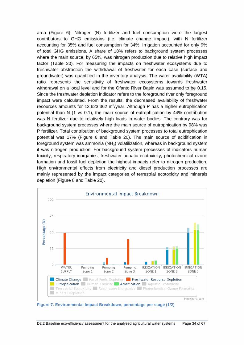
D2.2 Baseline eco-efficiency assessment for the analysed agricultural water systems Page 34 of 67
area (Figure 6). Nitrogen (N) fertilizer and fuel consumption were the largest
contributors to GHG emissions (i.e. climate change impact), with N fertilizer
accounting for 35% and fuel consumption for 34%. Irrigation accounted for only 9%
of total GHG emissions. A share of 18% refers to background system processes
where the main source, by 65%, was nitrogen production due to relative high impact
factor (Table 20). For measuring the impacts on freshwater ecosystems due to
freshwater abstraction the withdrawal of freshwater for each case (surface and
groundwater) was quantified in the inventory analysis. The water availability (WTA)
ratio represents the sensitivity of freshwater ecosystems towards freshwater
withdrawal on a local level and for the Ofanto River Basin was assumed to be 0.15.
Since the freshwater depletion indicator refers to the foreground river only foreground
impact were calculated. From the results, the decreased availability of freshwater
resources amounts for 13,623,362 m3/year. Although P has a higher eutrophication
potential than N (1 vs 0.1), the main source of eutrophication by 44% contribution
was N fertilizer due to relatively high loads in water bodies. The contrary was for
background system processes where the main source of eutrophication by 98% was
P fertilizer. Total contribution of background system processes to total eutrophication
potential was 17% (Figure 6 and Table 20). The main source of acidification in
foreground system was ammonia (NH3) volatilization, whereas in background system
it was nitrogen production. For background system processes of indicators human
toxicity, respiratory inorganics, freshwater aquatic ecotoxicity, photochemical ozone
formation and fossil fuel depletion the highest impacts refer to nitrogen production.
High environmental effects from electricity and diesel production processes are
mainly represented by the impact categories of terrestrial ecotoxicity and minerals
depletion (Figure 8 and Table 20).
Figure 7. Environmental Impact Breakdown, percentage per stage (1/2)
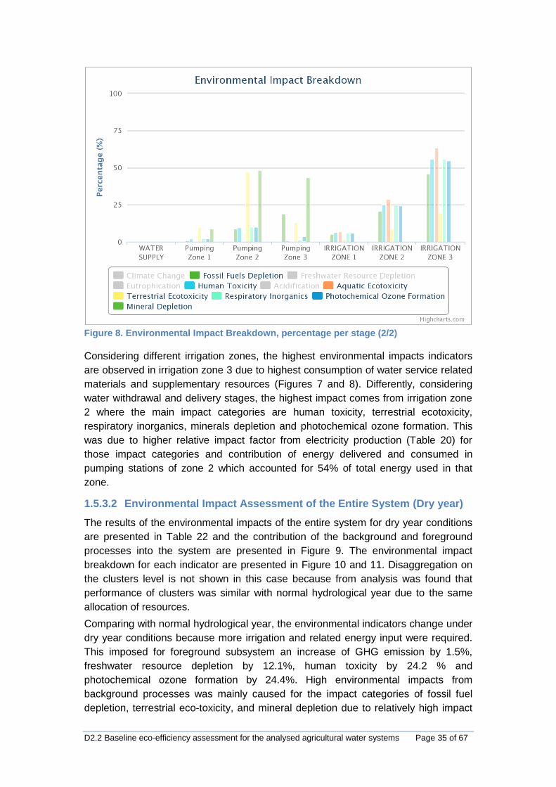
D2.2 Baseline eco-efficiency assessment for the analysed agricultural water systems Page 35 of 67
Figure 8. Environmental Impact Breakdown, percentage per stage (2/2)
Considering different irrigation zones, the highest environmental impacts indicators
are observed in irrigation zone 3 due to highest consumption of water service related
materials and supplementary resources (Figures 7 and 8). Differently, considering
water withdrawal and delivery stages, the highest impact comes from irrigation zone
2 where the main impact categories are human toxicity, terrestrial ecotoxicity,
respiratory inorganics, minerals depletion and photochemical ozone formation. This
was due to higher relative impact factor from electricity production (Table 20) for
those impact categories and contribution of energy delivered and consumed in
pumping stations of zone 2 which accounted for 54% of total energy used in that
zone.
1.5.3.2 Environmental Impact Assessment of the Entire System (Dry year)
The results of the environmental impacts of the entire system for dry year conditions
are presented in Table 22 and the contribution of the background and foreground
processes into the system are presented in Figure 9. The environmental impact
breakdown for each indicator are presented in Figure 10 and 11. Disaggregation on
the clusters level is not shown in this case because from analysis was found that
performance of clusters was similar with normal hydrological year due to the same
allocation of resources.
Comparing with normal hydrological year, the environmental indicators change under
dry year conditions because more irrigation and related energy input were required.
This imposed for foreground subsystem an increase of GHG emission by 1.5%,
freshwater resource depletion by 12.1%, human toxicity by 24.2 % and
photochemical ozone formation by 24.4%. High environmental impacts from
background processes was mainly caused for the impact categories of fossil fuel
depletion, terrestrial eco-toxicity, and mineral depletion due to relatively high impact

D2.2 Baseline eco-efficiency assessment for the analysed agricultural water systems Page 36 of 67
factors for diesel production. Minor change was found for eutrophication due to low
impact factor for resource production processes and no changes in fertilizer
application.
Table 22. Environmental Impacts of the Study System (Dry Year)
Indicator Value (Unit)
Foreground Value (Unit)
Background Value(Unit)
Type I Indicator (per kg
product)
Type II Indicator (per m
3
water used)
Climate Change (tCO2eq)
78,072,936 64,439,461 13,633,474 0.1364 0.9442
Fossil Fuels Depletion (MJ)
7,040,670 0 7,040,670 0.0123 0.0852
Freshwater Resource Depletion (m
3)
15,271,330 15,271,330 0 0.0267 0.1847
Eutrophication (kgPO4eq)
879,040 727,182 151,858 0.0015 0.0106
Human Toxicity (kg1,4-DBeq)
3,813,165 166 3,812,998 0.0067 0.0461
Acidification (kgSO2eq)
1,113,110 934,438 178,672 0.0019 0.0135
Aquatic Ecotoxicity (kg1,4-DBeq)
1,251,467 0 1,251,467 0.0022 0.0151
Terrestrial Ecotoxicity (kg1,4-DBeq)
8,335 0 8,335 0.0000 0.0001
Respiratory Inorganics (kgPM10,eq)
24,313 0 24,313 0.0000 0.0003
Photochemical Ozone Formation (kgC2H4,eq)
7,890 45 7,845 0.0000 0.0001
Mineral Depletion (kgFe-eq)
2,291 0 2,291 0.0000 0.0000
Figure 9. Contribution of Foreground and Background Systems in the environmental impact categories for dry year conditions
On the farm level (considering the irrigation zones), the most significant
environmental impacts were observed in irrigation zone 3 due to highest
consumption of water service related materials and supplementary resources.
Similarly to the normal hydrological year, when considering the water distribution

D2.2 Baseline eco-efficiency assessment for the analysed agricultural water systems Page 37 of 67
stages and withdrawals (pumping zones), the highest impact was observed in
irrigation zone 2 for impact categories of human toxicity, terrestrial eco-toxicity,
respiratory inorganics, and photochemical ozone formation. Differences were
observed for the impact category of mineral depletion where the main source was
irrigation zone 3 due to highest impact from diesel production for this category.
Figure 10. Environmental Impact Breakdown, percentage per stage (1/2) - Dry Year
Figure 11. Environmental Impact Breakdown, percentage per stage (2/2) - Dry Year
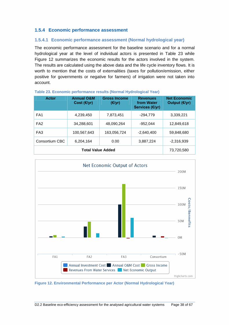
D2.2 Baseline eco-efficiency assessment for the analysed agricultural water systems Page 38 of 67
1.5.4 Economic performance assessment
1.5.4.1 Economic performance assessment (Normal hydrological year)
The economic performance assessment for the baseline scenario and for a normal
hydrological year at the level of individual actors is presented in Table 23 while
Figure 12 summarizes the economic results for the actors involved in the system.
The results are calculated using the above data and the life cycle inventory flows. It is
worth to mention that the costs of externalities (taxes for pollution/emission, either
positive for governments or negative for farmers) of irrigation were not taken into
account.
Table 23. Economic performance results (Normal Hydrological Year)
Actor Annual O&M Cost (€/yr)
Gross Income (€/yr)
Revenues from Water
Services (€/yr)
Net Economic Output (€/yr)
FA1 4,239,450 7,873,451 -294,779 3,339,221
FA2 34,288,601 48,090,264 -952,044 12,849,618
FA3 100,567,643 163,056,724 -2,640,400 59,848,680
Consortium CBC 6,204,164 0.00 3,887,224 -2,316,939
Total Value Added 73,720,580
Figure 12. Environmental Performance per Actor (Normal Hydrological Year)

D2.2 Baseline eco-efficiency assessment for the analysed agricultural water systems Page 39 of 67
The Total Value Added (TVA) to the product from the water use of the Sinistra Ofanto
irrigation system was estimated about 73.7 M€ or 2190 €/ha. Overall, the results
indicate that the total value added of the system greatly depends upon the yields
achieved, i.e. upon the level of water use. From Figure 12, it can be observed that
the highest benefits are gained in FA3 with 2935 €/ha due to largest gross income
which is the consequence of more profitable cropping pattern and greater irrigation
water supply (3023 m3/ha) in respect to zones 1 and 2 (895 and 1751 m3/ha).
Despite having a smaller surface in comparison with zone 2 and high land occupation
of wheat, zone 1 shows a better economic performance due to lower unitary life cycle
cost (i.e. production cost) which depends on cropping pattern. In fact, in zone 2, the
large areas are cultivated with table grape which has high production cost (6556
€/ha). On the contrary, in zone 1, the large areas are cultivated with wheat under
rainfed and with low production cost (548 €/ha). The costs for groundwater pumping
represents about 13% of total expenditures, varying proportionally between zones
according to water demand. The total costs for CBC estimated for the reference year
2007 were about 6.2 million € where fixed cost was about 4.34 million € (70% of
total) while the variable cost of water distribution was 1.86 million € (30% of total).
The analysis of the CBC economic balance shows a large difference between the
cost of water and revenues with a negative balance of more than 2 million €. The
lowest cost of the CBC for supplying water is relative to the irrigation zone 1,
although this zone has the biggest unitary cost. The low total cost in this zone is due
to the lower volume of water supplied (2 Mm3) in respect to zones 2 and 3 (8.7 and
25.8 Mm3, respectively).
1.5.4.2 Economic performance assessment (Dry year)
The economic performance assessment for baseline scenario for dry year conditions
at the level of individual actors is presented in Table 24 while Figure 13 summarizes
the economic results for actors involved.
Table 24. Economic performance results (Dry Year)
Actor Annual O&M Cost (€/yr)
Gross Income (€/yr)
Revenues from Water Services
(€/yr)
Net Economic Output (€/yr)
FA1 4,365,073.70 7,234,120.60 -294,779.28 2,574,267.61
FA2 35,327,381.66 45,101,881.88 -952,044.85 8,822,455.37
FA3 103,797,820.34 158,306,858.08 -2,640,400.84 51,868,636.90
Consortium CBC 6,204,164.16 0.00 3,887,224.97 -2,316,939.19
Total Value Added 60,948,420
The Total Value Added (TVA) of the Sinistra Ofanto irrigation system for dry year was
estimated about 60.9 M€ or 1811 €/ha. Differences between both average and high
water demand conditions were very significant. With regard to average year, in dry
year TVA decreased by 12.7 M€ or 21 %. Life cycle (production) costs were
increased by 3.1% due to greater water withdrawals to compensate the reduction of
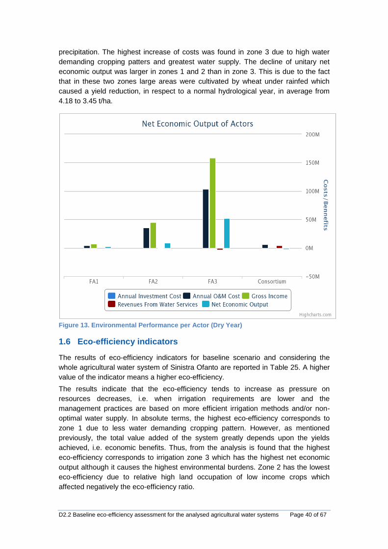
D2.2 Baseline eco-efficiency assessment for the analysed agricultural water systems Page 40 of 67
precipitation. The highest increase of costs was found in zone 3 due to high water
demanding cropping patters and greatest water supply. The decline of unitary net
economic output was larger in zones 1 and 2 than in zone 3. This is due to the fact
that in these two zones large areas were cultivated by wheat under rainfed which
caused a yield reduction, in respect to a normal hydrological year, in average from
4.18 to 3.45 t/ha.
Figure 13. Environmental Performance per Actor (Dry Year)
1.6 Eco-efficiency indicators
The results of eco-efficiency indicators for baseline scenario and considering the
whole agricultural water system of Sinistra Ofanto are reported in Table 25. A higher
value of the indicator means a higher eco-efficiency.
The results indicate that the eco-efficiency tends to increase as pressure on
resources decreases, i.e. when irrigation requirements are lower and the
management practices are based on more efficient irrigation methods and/or non-
optimal water supply. In absolute terms, the highest eco-efficiency corresponds to
zone 1 due to less water demanding cropping pattern. However, as mentioned
previously, the total value added of the system greatly depends upon the yields
achieved, i.e. economic benefits. Thus, from the analysis is found that the highest
eco-efficiency corresponds to irrigation zone 3 which has the highest net economic
output although it causes the highest environmental burdens. Zone 2 has the lowest
eco-efficiency due to relative high land occupation of low income crops which
affected negatively the eco-efficiency ratio.
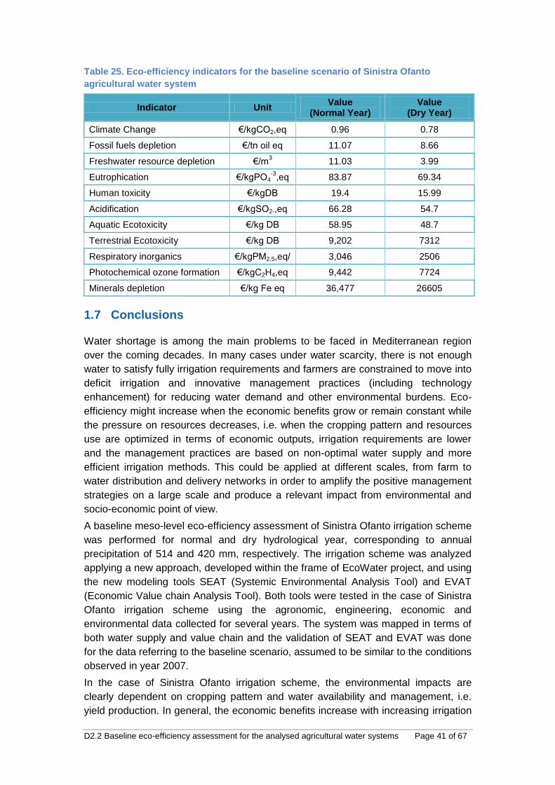
D2.2 Baseline eco-efficiency assessment for the analysed agricultural water systems Page 41 of 67
Table 25. Eco-efficiency indicators for the baseline scenario of Sinistra Ofanto
agricultural water system
Indicator Unit Value
(Normal Year) Value
(Dry Year)
Climate Change €/kgCO2,eq 0.96 0.78
Fossil fuels depletion €/tn oil eq 11.07 8.66
Freshwater resource depletion €/m3 11.03 3.99
Eutrophication €/kgPO4-3
,eq 83.87 69.34
Human toxicity €/kgDB 19.4 15.99
Acidification €/kgSO2-,eq 66.28 54.7
Aquatic Ecotoxicity €/kg DB 58.95 48.7
Terrestrial Ecotoxicity €/kg DB 9,202 7312
Respiratory inorganics €/kgPM2.5,eq/ 3,046 2506
Photochemical ozone formation €/kgC2H4,eq 9,442 7724
Minerals depletion €/kg Fe eq 36,477 26605
1.7 Conclusions
Water shortage is among the main problems to be faced in Mediterranean region
over the coming decades. In many cases under water scarcity, there is not enough
water to satisfy fully irrigation requirements and farmers are constrained to move into
deficit irrigation and innovative management practices (including technology
enhancement) for reducing water demand and other environmental burdens. Eco-
efficiency might increase when the economic benefits grow or remain constant while
the pressure on resources decreases, i.e. when the cropping pattern and resources
use are optimized in terms of economic outputs, irrigation requirements are lower
and the management practices are based on non-optimal water supply and more
efficient irrigation methods. This could be applied at different scales, from farm to
water distribution and delivery networks in order to amplify the positive management
strategies on a large scale and produce a relevant impact from environmental and
socio-economic point of view.
A baseline meso-level eco-efficiency assessment of Sinistra Ofanto irrigation scheme
was performed for normal and dry hydrological year, corresponding to annual
precipitation of 514 and 420 mm, respectively. The irrigation scheme was analyzed
applying a new approach, developed within the frame of EcoWater project, and using
the new modeling tools SEAT (Systemic Environmental Analysis Tool) and EVAT
(Economic Value chain Analysis Tool). Both tools were tested in the case of Sinistra
Ofanto irrigation scheme using the agronomic, engineering, economic and
environmental data collected for several years. The system was mapped in terms of
both water supply and value chain and the validation of SEAT and EVAT was done
for the data referring to the baseline scenario, assumed to be similar to the conditions
observed in year 2007.
In the case of Sinistra Ofanto irrigation scheme, the environmental impacts are
clearly dependent on cropping pattern and water availability and management, i.e.
yield production. In general, the economic benefits increase with increasing irrigation
D2.2 Baseline eco-efficiency assessment for the analysed agricultural water systems Page 42 of 67
water supply and moving to the more commercial cropping pattern (as in the case of
irrigation zone 3). However, it is increasing the environmental burden because
greater water service related materials and supplementary resources are used. In
general, the hydrological conditions play a relevant role in the eco-efficiency
assessment because more precipitation usually means (at least for winter crops)
lower irrigation requirements and therefore less consumption of resources. However,
in the case of a dry year, with annual precipitation of around 400mm or less, several
problems could occur in terms of both economic and environmental sustainability
(including an excessive depletion of the aquifers).
As a whole and in the case of a normal hydrological year, the results of this study
confirm that the system is performing below the expected sustainability limits
because the groundwater withdrawal is greater than the recharge for about 16.1 Mm3
per year which indicates a clear trend of reduction of water availability in the region
and worsening of environmental conditions. Therefore, the introduction of new
technologies and their uptake are urgently needed to contribute in the improvement
of actual situation and the eco-efficiency of the system. These improvements are
even more relevant for the system running under dry conditions. The upgrading of
the value chain through innovative technologies should aim at improving the key
indicators which are related to the use of non-renewable energy sources, fresh water
abstraction and chemicals use (Human Toxicity, Fresh water and Terrestrial Eco-
toxicity, Freshwater depletion, Fossil fuels depletion, Acidification). Indicative options
towards that are the following:
The adaptation of more efficient irrigation technologies that will reduce energy
and fresh water consumption on the agricultural use level. This will result to:
o Decrease of the “climate change” eco-efficiency indicator and of the
indicators related to the electricity production (human toxicity,
terrestrial and aquatic ecotoxicity); and
o Reduction of fresh water depletion indicator.
Reduction of the discharge of pollutants due to the use of less toxic chemicals
(fertilizers) which will affect the “eutrophication” and “acidification” eco-
efficiency indicators.

D2.2 Baseline eco-efficiency assessment for the analysed agricultural water systems Page 43 of 67
2 Baseline eco-efficiency assessment of the Monte Novo
Case Study
2.1 Introduction
The baseline eco-efficiency assessment of the Case Study # 2: Monte Novo Irrigation
Area – Portugal was performed taking into account the five phases of an eco-
efficiency assessment (ISO, 2012): (i) Goal and Scope Definition, (ii) Environment
Assessment, (iii) Value Assessment, (iv) Quantification of Eco-efficiency and (v)
Interpretation. The eco-efficiency assessment is a quantitative tool which enables the
study of the environmental impacts in this specific case, of an agricultural product
along with its value.
The environmental impacts were evaluated using a Life Cycle Assessment (LCA)
oriented approach, based on the creation of an inventory of elementary flows
(relevant energy, resource inputs and environmental releases) that allows the Life
Cycle Impact Assessment (LCIA); identification and evaluation of the potential
environmental impacts associated with identified inputs and releases.
The value assessment was performed considering the full life cycle of the product
system. The values were calculated in monetary terms (€) and are expressed
through costs, price, willingness to pay, added value, profit, etc.). The Total Value
Added (TVA) was the economic performance indicator used.
Finally, the quantification of eco-efficiency was determined by relating the results of
the environmental assessment to the results of the value assessment, based on the
“eco-efficiency equation” (Figure 14). By the end of the study, 11 Eco-Efficiency
Indicators (EEI) were obtained, one for each environmental impact category, as it will
be hereafter presented.
Eco-efficiency =Value of product or service
Environmental impacts
Enhancing the value
Reducing the impacts
Figure 14. The eco-ifficiency equation.
2.2 Goal and Scope Definition
2.2.1 Objectives
The main goal of this study is the assessment of the environmental and economic
impacts and the eco-efficiency performance associated with the water value chain in
the Monte Novo case study. The analysis is targeted on a meso-level that
encompasses the water supply and water use chains and entails the consideration of
the interrelations among the heterogeneous actors.

D2.2 Baseline eco-efficiency assessment for the analysed agricultural water systems Page 44 of 67
The assessment is performed in the baseline scenario which represents the
reference point for benchmarking enhancements resulting from the upgrade of the
value chain through the introduction of innovative technologies, which will be
examined in a later stage.
2.2.2 System boundaries
The main stages of the Monte Novo case study are the water abstraction, water
distribution, water use and disposal. Table 26 presents the stages, processes and
technologies corresponding to the water supply chain presented in Figure 15.
Table 26. Stages, processes and technologies in the Monte Novo case study.
Stage 1: Water abstraction
Process 1: primary network
Technology 1: pumping station
Technology 2: conveyance canals and ducts
Stage 2: Water distribution
Process 2: secondary network – low pressure
Technology 3: regulating reservoirs
Process 3: secondary network – high pressure
Technology 1: pumping station
Technology 3: regulating reservoirs
Stage 3: Water use
Process 4: farmers – low pressure (olives, maize, pastures)
Technology 4: drip irrigation (olives – intensive and super intensive)
Technology 5: sprinkler irrigation (maize, pastures)
Process 5: farmers – high pressure (olives, maize, pastures)
Technology 4: drip irrigation (olives – intensive and super intensive)
Technology 5: sprinkler irrigation (maize, pastures)
Stage 4: Disposal
Residual water discharged to the environment (SW and GW)
More specifically, one can indicate that:
the primary network corresponds to water abstraction in the Alqueva reservoir
(main storage reservoir of the system), elevation and water transport to the
secondary networks;
the secondary network includes the regulating storage made through several
reservoirs (R1, R2, R3, R4, R4.1), the elevation stage and the water
distribution to the different irrigated farms considered;
the farmers (users) in the Monte Novo case study are represented by means
of the most representative crops in the area.

D2.2 Baseline eco-efficiency assessment for the analysed agricultural water systems Page 45 of 67
Figure 15. Stages, processes and involved actors in the water supply chain of the Monte Novo Case Study.
Three actors are directly involved in the system:
EDIA (“Empresa para o Desenvolvimento das Infraestruturas de Alqueva).
EDIA is the entity responsible for the management and development of the
Alqueva multipurpose project, including the operation of primary and
secondary irrigation network where the Monte Novo irrigation perimeter is
included.
AB Monte Novo (“Associação de Beneficiários de Monte Novo”), which
represents all the farmers which are connected to the Alqueva water
distribution system from EDIA, and
Farmers that will benefit from the irrigation networks, more specifically, FEA
(“Fundação Eugénio de Almeida”) and ODS (“Olivais do Sul”). The main
crops of Fundação Eugénio de Almeida are vineyards and olives. Olivais do
Sul are specialized in olive growing and olive oil production. The olive
production is made using both intensive and super-intensive methods.
As referred above, the environmental and eco-efficiency assessment incorporating a
life cycle oriented approach along the water supply chain considers the
environmental impacts of: the input resources and materials, the energy use and the
agricultural facilities. Regarding the system boundary used for the LCA, the “cradle-
to-gate” analysis was considered, which is an assessment of a partial product life
cycle, i.e. starting from the extraction of primary resources (cradle) to the point that
products leave the agricultural system boundaries (before the transportation to the
consumer). However, no use or end life is taking into account.
With this approach, the system’s boundaries of the Monte Novo Case Study were
identified, emphasizing that the foreground and background systems have to be
distinguished:

D2.2 Baseline eco-efficiency assessment for the analysed agricultural water systems Page 46 of 67
the foreground system corresponds to the set of processes whose selection
or mode of operation is affected directly by decisions based on the study;
the background system includes all other activities which delivers energy
and raw materials to the foreground system, usually via a homogeneous
market so that individual plants and operations cannot be identified.
Figure 16 presents these concepts applied to the Monte Novo case study, according
to the stages presented in Table 26.
Figure 16. Life Cycle Diagram of the Study System including Foreground and Background Systems.
Table 27. Foreground and Background processes of the Monte Novo Irrigation
Scheme.
Type of Process Name
Foreground 1. Water abstraction – primary network
2. Water distribution – secondary network (low pressure)
3. Water distribution – secondary network (high pressure)
4. Water use – farmers (low pressure)
5. Water use – farmers (high pressure)
6. Disposal
Background 1. Electricity production
2. Nitrogen fertilizer manufacturing process
3. Phosphorus fertilizer manufacturing process
The Life Cycle Assessment approach considers the impacts from elementary flows
entering the system and also the direct emission to the environment from the
operations of the study system itself. The foreground system was focused on all the
stages along the water value chain where supplementary resources (agro-chemicals
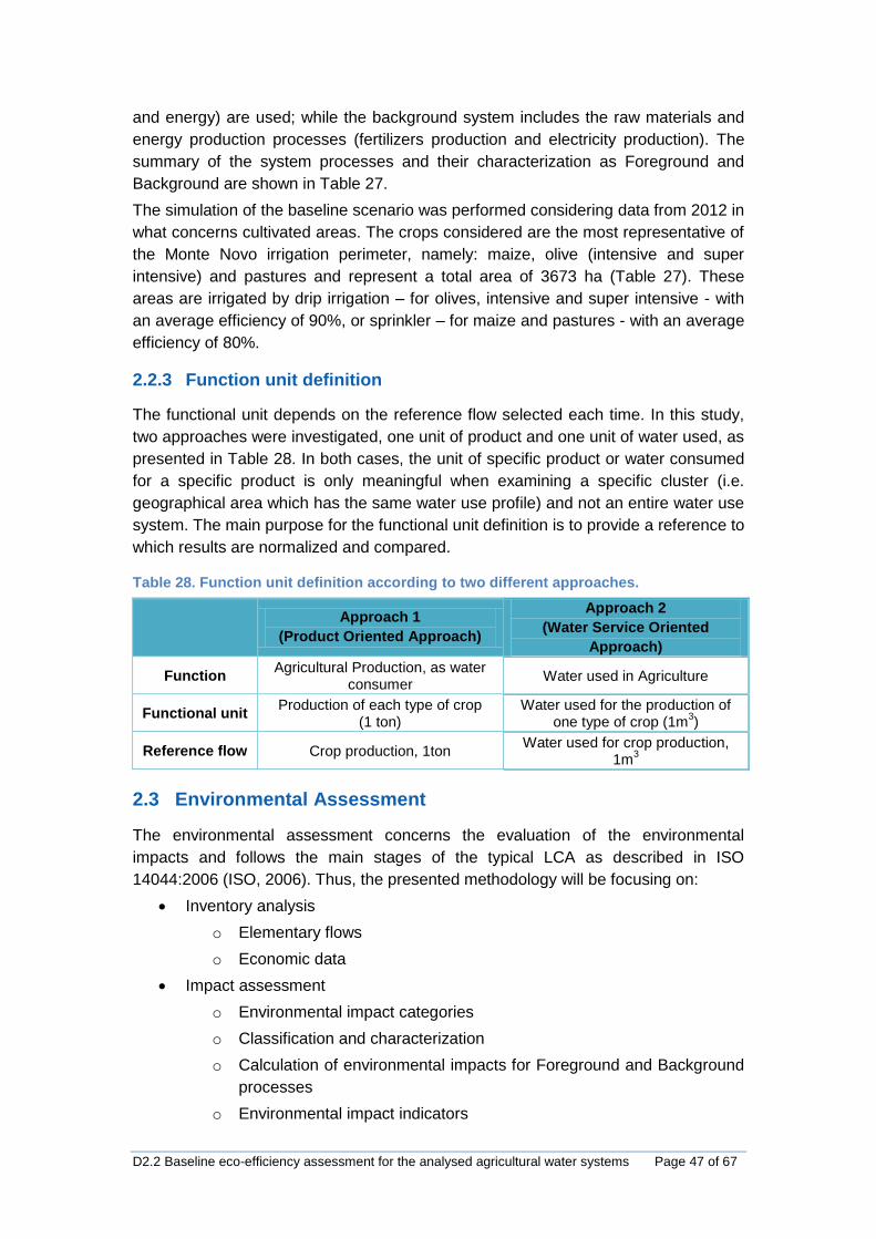
D2.2 Baseline eco-efficiency assessment for the analysed agricultural water systems Page 47 of 67
and energy) are used; while the background system includes the raw materials and
energy production processes (fertilizers production and electricity production). The
summary of the system processes and their characterization as Foreground and
Background are shown in Table 27.
The simulation of the baseline scenario was performed considering data from 2012 in
what concerns cultivated areas. The crops considered are the most representative of
the Monte Novo irrigation perimeter, namely: maize, olive (intensive and super
intensive) and pastures and represent a total area of 3673 ha (Table 27). These
areas are irrigated by drip irrigation – for olives, intensive and super intensive - with
an average efficiency of 90%, or sprinkler – for maize and pastures - with an average
efficiency of 80%.
2.2.3 Function unit definition
The functional unit depends on the reference flow selected each time. In this study,
two approaches were investigated, one unit of product and one unit of water used, as
presented in Table 28. In both cases, the unit of specific product or water consumed
for a specific product is only meaningful when examining a specific cluster (i.e.
geographical area which has the same water use profile) and not an entire water use
system. The main purpose for the functional unit definition is to provide a reference to
which results are normalized and compared.
Table 28. Function unit definition according to two different approaches.
Approach 1
(Product Oriented Approach)
Approach 2
(Water Service Oriented
Approach)
Function Agricultural Production, as water
consumer Water used in Agriculture
Functional unit Production of each type of crop
(1 ton) Water used for the production of
one type of crop (1m3)
Reference flow Crop production, 1ton Water used for crop production,
1m3
2.3 Environmental Assessment
The environmental assessment concerns the evaluation of the environmental
impacts and follows the main stages of the typical LCA as described in ISO
14044:2006 (ISO, 2006). Thus, the presented methodology will be focusing on:
Inventory analysis
o Elementary flows
o Economic data
Impact assessment
o Environmental impact categories
o Classification and characterization
o Calculation of environmental impacts for Foreground and Background
processes
o Environmental impact indicators

D2.2 Baseline eco-efficiency assessment for the analysed agricultural water systems Page 48 of 67
o Cluster and area indicators
2.3.1 Inventory analysis
2.3.1.1 Elementary flows
The LCI analysis involves the creation of an inventory of flows entering and leaving
every process in the foreground system. In the Monte Novo case study, the data
requirement is focused on:
i) Foreground data (direct emissions and water abstraction) extracted from SEAT
model:
Nitrogen to Water
Phosphorus to Water
Water consumption
ii) Characterization factors for background processes:
Electricity production
Nitrogen fertilizer manufacturing process
Phosphorus fertilizer manufacturing process
For the next stage of the environmental assessment – the impact assessment –the
main inputs and outputs coming from SEAT model were collected, for the baseline
scenario. Table 29 presents the different resources involved in the Monte Novo case
study.
Table 29. Resources of the Monte Novo case study.
Category Symbol Resource
Water service related materials w Water
Supplementary resources r1 Energy
r2 Fertilizer (Phosphorus)
r3 Fertilizer (Nitrogen)
r4 Irrigated area
Emissions e1 CO2
e2 Wastewater
e3 Nitrogen to water
e4 Phosphorus to water
Products p1 Maize (grain)
p2 Olives
p3 Pastures
The corresponding elementary flows and associated quantities are depicted in Table
30. The information presented was extracted from SEAT model and all flows are
referred to annual average values.

D2.2 Baseline eco-efficiency assessment for the analysed agricultural water systems Page 49 of 67
Table 30. Life cycle inventory flows of the Monte Novo Irrigation Scheme (from SEAT).
Category Material Quantity
Water service related materials Water 24,904,792 m3
Supplementary resources Energy 13,370,830 kWh
Fertilizer (Phosphorus) 587,680 kg
Fertilizer (Nitrogen) 330,570 kg
Irrigated area 3,673 m2
Emissions CO2 6,779,011 kg
Wastewater 6,546,100 m3
Nitrogen to water 110,190 kg
Phosphorus to water 7,346 kg
Products Maize (grain) 20,055 ton
Olives 18,360 ton
Pastures 5,090 ton
2.3.1.2 Economic data
Table 31 summarizes the economic data considered in the study.
Table 31. Unit costs of raw materials and supplementary resources.
Cost category Item Amount
Cost
Water – LP 0.0258 €/m3
Water – HP 0.042 €/m3
Electricity 0.118 €/kWh
Fertilizer (N) 2.34 €/kg
Fertilizer (P) 2.34 €/kg
Benefit
Maize (grain) 220 €/ton
Olive 234 €/ton
Pastures 135 €/ton
2.3.2 Impact Assessment
2.3.3 Environmental impact categories
The assessment of the environmental performance of the EcoWater meso-level
water use system, and specifically, of the Monte Novo Case Study, follows a life-
cycle oriented approach using the midpoint impact categories presented in Table 32,
and according to each selected Impact Assessment Method.

D2.2 Baseline eco-efficiency assessment for the analysed agricultural water systems Page 50 of 67
Table 32. Midpoint impact categories and impact assessment methods.
Impact Category Unit Impact Assessment Method
Climate change kgCO2, eq CML 2001
Eutrophication kgPO43-
, eq CML 2001
Acidification kgSO2-,eq CML 2001
Human toxicity kg DB CML 2001
Respiratory inorganics kgPM10, eq Trace
Fresh water aquatic ecotoxicity kg DB CML 2001
Ecotoxicity Terrestrial kg DB CML 2001
Photochemical ozone formation kgC2H4, eq CML 2001
Minerals depletion kg Fe, eq Recipe
Fossil fuels depletion kg oil, eq Recipe
Freshwater depletion m3 (Milà i Canals et al., 2009)
2.3.3.1 Classification and characterization
During the classification phase, the results of the inventory, expressed as elementary
flows, are assigned to impact categories according to the ability of resource/emission
to contribute to different environmental problems.
The characterization factors for each Impact Assessment Method, according to the
Impact Categories that they cover (Table 32), were collected. Tables 33 and 35
present the characterization factors which are used for the estimation of the impact of
the foreground systems and the environmental impact factors for the background
processes, respectively.
Table 33. Characterization factors of foreground elementary flows.
Impact category Unit N to water
(per kg)
P to water
(per kg)
Water (per
m3)
Climate change kg CO2, eq
Eutrophication kg PO4-3
, eq 0.42 3.06
Acidification kg SO2-, eq
Human toxicity kg 1,4-DB, eq
Respiratory inorganics kgPM10, eq
Aquatic ecotoxicity kg DB
Terrestrial ecotoxicity kg DB
Photochemical ozone formation kgC2H4, eq
Minerals depletion kg Fe, eq
Fossil fuels depletionn kg oil, eq
Freshwater depletion m
3
0.15

D2.2 Baseline eco-efficiency assessment for the analysed agricultural water systems Page 51 of 67
Table 34. Background processes and relevant data sources.
Process Data Sources
Electricity Production ELCD database (Process Name: Electricity Mix, AC, consumption
mix, at consumer, 230V PT)
Nitrogen fertilizer
production
USLCI database (Process name: Nitrogen fertilizer, production mix,
at plant/kg/US)
Phosphorus fertilizer
production
USLCI database (Process Name: Phosphorous fertilizer, production
mix, at plant/kg/US)
Table 35. Environmental impact factors for background processes.
Impact category Unit
Electricity
Production
(per kWh)
Nitrogen
Fertilizer
Productio
n (per kg)
Phosphorus
Fertilizer
Production
(per kg)
Climate change kg CO2, eq 0.80139 1.93006 0.39097
Eutrophication kg PO4-3
, eq 0.00030 0.00035 0.06724
Acidification kg SO2-, eq 0.00606 0.02339 0.02197
Human toxicity kg 1,4-DB, eq 0.06648 0.64951 0.16316
Respiratory inorganics kgPM10, eq 0.00095 0.00314 0.00300
Aquatic ecotoxicity kg DB 0.00311 0.22896 0.08853
Terrestrial ecotoxicity kg DB 0.00154 0.00022 0.00063
Photochemical ozone
formation kgC2H4, eq 0.00025 0.00100 0.00093
Minerals depletion kg Fe, eq 0.00018 0.00000 0.00000
Fossil fuels depletionn kg oil, eq 0.20155 0.97804 0.14833
2.3.3.2 Calculation of environmental impacts for foreground and
background processes
The environmental impact was calculated by multiplying the elementary flows from
the inventory analysis with the characterization factors. This method was applied for
each impact category and the environmental impact assessment for an impact
category can be estimated as the sum of the foreground and background processes.
The results of the environmental impacts, for the foreground and background
systems, are presented in Table 36. For the foreground, two environmental indicators
are relevant: eutrophication and freshwater depletion. On the other hand, for the
background system, all the impact categories were considered.
Regarding the foreground system, it is possible to verify that eutrophication and
water depletion impact categories are the only ones affected. The eutrophication
value is a result of the nitrogen and phosphorus flows to surface water bodies and
groundwater, due to the use of N and P fertilizers in agricultural use stages, whereas
the freshwater depletion expresses the water abstraction to satisfy the irrigation
requirements at the farmer’s level.

D2.2 Baseline eco-efficiency assessment for the analysed agricultural water systems Page 52 of 67
Table 36. Environmental impacts from foreground and background systems.
Environmental
Indicators Unit
Value
Background
from
electricity
Background
from other
processes
Foreground Total
Climate change ton CO2, eq 10,715 1,264 0 11,979
Eutrophication kg PO43-
, eq 3,952 22,435 68,759 95,145
Acidification kg SO2-,eq 81,054 21,007 0 102,061
Human toxicity ton DB 889 436 0 1,324
Respiratory
inorganics kg PM10, eq 12,767 2,839 0 15,606
Aquatic ecotoxicity ton DB 42 164 0 205
Terrestrial ecotoxicity kg DB 20,542 338 0 20,880
Photochemical ozone
formation kg C2H4, eq 3,396 897 0 4,292
Minerals depletion kg Fe, eq 2,443 0 0 2,443
Fossil fuels depletion ton oil, eq 2,695 624 0 3,319
Freshwater depletion m3 0 0 3,735,719 3,735,719
Figure 17 summarizes the values presented in Table 36, and enables their better
interpretation. In fact, it is possible to highlight the high environmental effect from the
electricity production for most of the impact categories, namely, climate change,
acidification, human toxicity, respiratory inorganics, terrestrial ecotoxicity,
photochemical ozone formation, mineral depletion and fossil fuels depletion.
Moreover, it is possible to verify the considerable contribution of the fertilizer
manufacturing processes (“background from other processes”) in the freshwater
aquatic ecotoxicity due to the presence of toxic substances.
Figure 17. Environmental impact assessment for foreground and background systems.

D2.2 Baseline eco-efficiency assessment for the analysed agricultural water systems Page 53 of 67
2.3.3.3 Environmental impacts indicators
The environmental impact indicators were calculated by expressing the
environmental impacts per unit of a product or per unit of water used (depending on
the choice of functional unit). In this case study, both indicators are presented,
following the two approaches:
Type I (per ton of drop production)
Type II (per m3 of water used for crop production).
The Type I impact indicators are presented in the graphs presented in Figure 18.
a) b)
c) d)
e) f)
g) h)
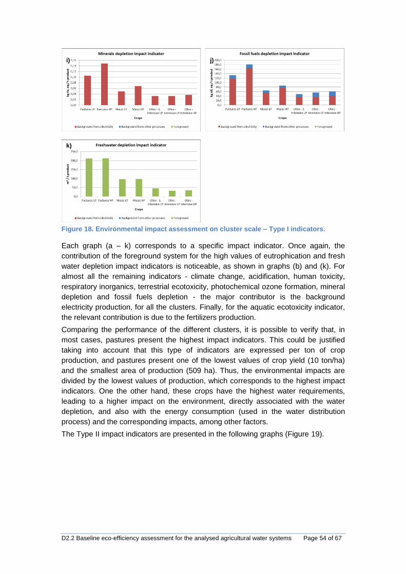
D2.2 Baseline eco-efficiency assessment for the analysed agricultural water systems Page 54 of 67
Figure 18. Environmental impact assessment on cluster scale – Type I indicators.
Each graph (a – k) corresponds to a specific impact indicator. Once again, the
contribution of the foreground system for the high values of eutrophication and fresh
water depletion impact indicators is noticeable, as shown in graphs (b) and (k). For
almost all the remaining indicators - climate change, acidification, human toxicity,
respiratory inorganics, terrestrial ecotoxicity, photochemical ozone formation, mineral
depletion and fossil fuels depletion - the major contributor is the background
electricity production, for all the clusters. Finally, for the aquatic ecotoxicity indicator,
the relevant contribution is due to the fertilizers production.
Comparing the performance of the different clusters, it is possible to verify that, in
most cases, pastures present the highest impact indicators. This could be justified
taking into account that this type of indicators are expressed per ton of crop
production, and pastures present one of the lowest values of crop yield (10 ton/ha)
and the smallest area of production (509 ha). Thus, the environmental impacts are
divided by the lowest values of production, which corresponds to the highest impact
indicators. One the other hand, these crops have the highest water requirements,
leading to a higher impact on the environment, directly associated with the water
depletion, and also with the energy consumption (used in the water distribution
process) and the corresponding impacts, among other factors.
The Type II impact indicators are presented in the following graphs (Figure 19).
i) j)
k)
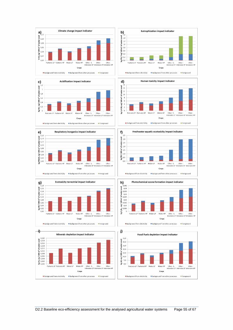
D2.2 Baseline eco-efficiency assessment for the analysed agricultural water systems Page 55 of 67
a) b)
c) d)
e) f)
g) h)
i) j)
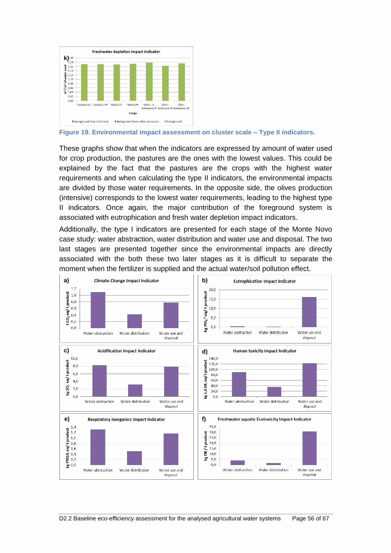
D2.2 Baseline eco-efficiency assessment for the analysed agricultural water systems Page 56 of 67
Figure 19. Environmental impact assessment on cluster scale – Type II indicators.
These graphs show that when the indicators are expressed by amount of water used
for crop production, the pastures are the ones with the lowest values. This could be
explained by the fact that the pastures are the crops with the highest water
requirements and when calculating the type II indicators, the environmental impacts
are divided by those water requirements. In the opposite side, the olives production
(intensive) corresponds to the lowest water requirements, leading to the highest type
II indicators. Once again, the major contribution of the foreground system is
associated with eutrophication and fresh water depletion impact indicators.
Additionally, the type I indicators are presented for each stage of the Monte Novo
case study: water abstraction, water distribution and water use and disposal. The two
last stages are presented together since the environmental impacts are directly
associated with the both these two later stages as it is difficult to separate the
moment when the fertilizer is supplied and the actual water/soil pollution effect.
k)
a) b)
c) d)
e) f)
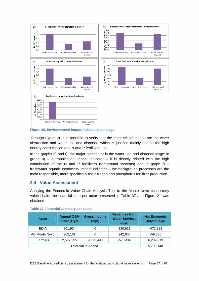
D2.2 Baseline eco-efficiency assessment for the analysed agricultural water systems Page 57 of 67
Figure 20. Environmental impact indicators per stage.
Through Figure 20 it is possible to verify that the most critical stages are the water
abstraction and water use and disposal, which is justified mainly due to the high
energy consumption and N and P fertilizers use.
In the graphs b) and f), the major contributor is the water use and disposal stage: in
graph b) – eutrophication impact indicator – it is directly related with the high
contribution of the N and P fertilizers (foreground systems) and in graph f) –
freshwater aquatic ecotoxicity impact indicator – the background processes are the
main responsible, more specifically the nitrogen and phosphorus fertilizer production.
2.4 Value Assessment
Applying the Economic Value Chain Analysis Tool to the Monte Novo case study
value chain, the financial data per actor presented in Table 37 and Figure 21 was
obtained.
Table 37. Financial summary per actor.
Actor Annual O&M
Cost (€/yr)
Gross Income
(€/yr)
Revenues from
Water Services
(€/yr)
Net Economic
Output (€/yr)
EDIA 801,934 0 330,611 -471,323
AB Monte Novo 302,161 0 242,805 -59,356
Farmers 2,582,255 9,395,490 -573,416 6,239,819
Total Value Added 5,709,140
g) h)
i) j)
k)

D2.2 Baseline eco-efficiency assessment for the analysed agricultural water systems Page 58 of 67
The Total Value Added (TVA), to the product from the water use, is the sum of the
net economic output of the actors, which is equal to 5,709,140 €.
Figure 21. Economic performance per actor.
2.5 Eco-Efficiency Quantification
The Eco-Efficiency Indicators are defined as the ratio of the economic performance
to the environmental performance of the system. Table 38 presents the eco-
efficiency indicators, corresponding to the 11 relevant environmental impact
categories.
Table 38. Eco-efficiency indicators.
Category impact Unit Eco-eficiency assessment
Climate change €/tnCO2, eq 476.6
Eutrophication €/kgPO43-
, eq 60.0
Acidification €/kgSO2-, eq 56.0
Human toxicity €/tnDB 4,310.5
Resp inorganics €/kgPM10, eq 365.8
Freshwater aquatic ecotoxicity €/kg DB 27,802.9
Terrestrial ecotoxicity €/ kg DB 273.4
Photochemical ozone formation €/kgC2H4, eq 1,330.1
Minerals depletion €/kg Fe, eq 2,337.2
Fossil fuels depletion €/tn oil, eq 1,720.3
Freshwater depletion €/m3 1.5
2.6 Conclusions
An upgrading of the water value chain should focus on the improvement of these
eco-efficiency indicators, directly related with the non-renewable sources
D2.2 Baseline eco-efficiency assessment for the analysed agricultural water systems Page 59 of 67
consumption: e.g. freshwater; and the chemicals use (such as the fertilizers
components). These contributors increase the environmental impacts associated with
agriculture (e.g. freshwater depletion, eutrophication, acidification, etc). The
improvement of the Monte Novo environmental performance should focus on:
Water supply chain technologies
Production chain technologies
o The adaptation of irrigation technologies that will reduce energy
consumption on the agricultural use level and subsequently
decreasing the “climate change” eco-efficiency indicator and the
indicators related with the electricity production (human toxicity,
terrestrial and freshwater ecotoxicity).
o Cultivation of crop types/production methods with lower agrochemical
needs, resulting to:
Reduction of the discharge of pollutants due to the use of
fertilizers
Decrease of the “eutrophication” eco-efficiency indicator

3 References Allen R.G., Pereira, L.S., Raes, D., Smith, M., 1998. Crop evapotranspiration. Guidelines for computing crop water requirements. Food and Agricultural Organization of the United Nations, Irrigation and Drainage Paper 56, FAO, Rome, pp.300.
Altieri, S., 1995. Sinistra Ofanto irrigation scheme : management and maintenance problems. In: L.S. Pereira (ed.). Bonifica, n. 1-2: 40-47.
Bouwman, A. F., Boumans, L. J. M., & Batjes, N. H. (2002). Modeling global annual N2O and NO emissions from fertilized fields. Global Biogeochemical Cycles, 16(4), 28-1.
Bouwman, A. F., Van Drecht, G., & Van der Hoek, K. W. (2005). Global and Regional Surface Nitrogen Balances in Intensive Agricultural Production Systems for the Period 1 ¼—2¼3¼. Pedosphere, 15(2), 137-155.
Consorzio per la Bonifica della Capitanata (CBC: www.consorzio.fg.it ).
D'Arcangelo G. (2005). Operation, maintenance and management of irrigation schemes in Italy: operational costs. In: Bogliotti C., Lamaddalena N., Lebdi F. and Todorovic M. (ed). Irrigation systems performance. Bari : CIHEAM, pp. 111-122. Options Méditerranéennes : Série B. Etudes et Recherches. DOI: 10.4408/IJEGE.2013-01.O-05
Eco-Water (2012). Background Note. Methodology Framework for the EcoWater Case Studies
Eco-Water (2012). Deliverable 1.1 Review and selection of indicators to beused in the Eco-Water case studies. In: Meso-level eco-efficiency indicators to assess technologies and their uptake in water use sectors.
Eco-Water (2012). Deliverable 1.4 Review of existing frameworks and tools for developing eco-efficiency indicators. In: Meso-level eco-efficiency indicators to assess technologies and their uptake in water use sectors.
Eco-Water (2012). Deliverable 2.1 Value chain mapping of agricultural water systems. In: Meso-level eco-efficiency indicators to assess technologies and their uptake in water use sectors.
Eggleston, H.S., Buendia, L., Miwa, K., Ngara, T., Tanabe, K., (2006). IPCC Guidelines for National Greenhouse Gas Inventories. Institute for Global Environmental Strategies, Hayama, Japan.
ELCD (2013), ELCD database, Retrieved from ELCD website: http://elcd.jrc.ec.europa.eu/ELCD3/processList.xhtml
FADN (2007). Farm Accountancy Data Network, Regional Database.
http://elcd.jrc.ec.europa.eu/ELCD3/processList.xhtml
Flury, K., Jungbluth, N., Frischknecht, R. (2011). Water Footprint: Methods, State of the Art, Outlook. Presentation and Discussion cewas, Willisau, Switzerland 22. September 2011.
Guinée, B. J. et al., 2001. Handbook on Life Cycle Assessment: Operational Guide to the ISO Standards. Dordrecht: Kluwer Academic Publishers.
Institute of Sciences of Food Production (ISPA), National Research Council (CNR), Italy (www.ispa.cnr.it)

D2.2 Baseline eco-efficiency assessment for the analysed agricultural water systems Page 61 of 67
ISO (2006), International Organization for Standardization, ISO 14044:2006 Environmental management -- Life cycle assessment – Requirements and guidelines, Genève, Switzerland.
Jones, C. D., Fraisse, C. W., & Ozores-Hampton, M. (2012). Quantification of greenhouse gas emissions from open field-grown Florida tomato production.Agricultural Systems, 113, 64-72.
Lal R. (2004). Carbon emission from farm operations. Environment international, 30(7): 981-990.
Maraseni, T. N., Cockfield, G., & Apan, A. (2007). A comparison of greenhouse gas emissions from inputs into farm enterprises in Southeast Queensland, Australia. Journal of Environmental Science and Health Part A, 42(1), 11-18.
Milà i Canals, L. et al., 2009. Assessing freshwater use impacts in LCA: Part I - inventory modelling and characterisation factors for the main impact pathways. International Journal of Life Cycle Assessment, 14 (1), p. 28–42.
Nussey, R. Farm carbon emissions, Western Australia, Australia. 2005.
Oueslati I., Zaccaria D., Vurro M. and Lamaddalena N. (2007). A methodology to relate groundwater salinity to irrigation delivery schedules: A case study in Southern Italy.
Pereira L. S., Teodoro P. R., Rodrigues P. N. and Teixeira J. L. (2003). Irrigation Scheduling Simulation: The Model Isareg. In:Rossi G., Cancelliere A., Pereira L., Oweis T., Shatanawi M. and Zairi A. (ed). Tools for Drought Mitigation in Mediterranean Regions. Springer Netherlands, pp. 161-180. Water Science and Technology Library.
Romanazzi A., and Polemio M (2013). Modeling of coastal karst aquifers for management support: A case study of Salento (Apulia, Italy). Italian Journal of Engineering Geology and Environment.
Sivapragasam C., Vasudevan G., Maran J., Bose C., Kaza S. and Ganesh N. (2009). Modeling evaporation-seepage losses for reservoir water balance in semi-arid regions. Water resources management, 23(5): 853-867.
USLCI (2013), USLCI database, Retrieved from US Life Cycle Inventory Database website, https://www.lcacommons.gov/nrel/search
van Schijndel, M. W., & Kuikman, P. J. (2007). Direct and indirect nitrous oxide emissions from agricultural soils, 1990-2003. Background document on the calculation method for the Dutch National Inventory Report.

D2.2 Baseline eco-efficiency assessment for the analysed agricultural water systems Page 62 of 67
Annex A – The results of environmental impact indicators at cluster level for a normal hydrological year (Case Study #1)
-
0,5
1,0
1,5
2,0
2,5
3,0
3,5
4,0
4,5
5,0
kgC
O₂e
q/m
³ o
f w
ate
r u
sed
Climate Change Impact Indicator
BACKGROUND
FOREGROUND
-
100,0
200,0
300,0
400,0
500,0
600,0
kgC
O₂e
q/t
on
of
pro
du
ct
Climate Change Impact Indicator
BACKGROUND
FOREGROUND
-
0,50
1,00
1,50
2,00
2,50
3,00
3,50
4,00
4,50
5,00
kgP
O₄/
ton
of
pro
du
ct
Eutrophication Potential Impact Indicator
BACKGROUND
FOREGROUND
-
0,005
0,010
0,015
0,020
0,025
0,030
0,035
0,040
0,045
0,050
kgP
O₄/
m³
of
wat
er
use
d
Eutrophication Potential Indicator
BACKGROUND
FOREGROUND

D2.2 Baseline eco-efficiency assessment for the analysed agricultural water systems Page 63 of 67
-
1,00
2,00
3,00
4,00
5,00
6,00
7,00kg
SO₂/
ton
of
pro
du
ct
Acidification Potential Impact Indicator
BACKGROUND
FOREGROUND
-
1,00
2,00
3,00
4,00
5,00
6,00
7,00
kgSO
₂/to
n o
f p
rod
uct
Acidification Potential Impact Indicator
BACKGROUND
FOREGROUND
-
5,0
10,0
15,0
20,0
25,0
30,0
35,0
40,0
kg 1
.4 d
B e
q /
ton
of
pro
du
ct
Humant Toxicity Potential Impact Indicator BACKGROUND
FOREGROUND
-
0,02
0,04
0,06
0,08
0,10
0,12
0,14
0,16
0,18
0,20
kg 1
.4 d
B e
q /
m³
of
wat
er
use
d
Human Toxicity Impact Indicator
BACKGROUND
FOREGROUND

D2.2 Baseline eco-efficiency assessment for the analysed agricultural water systems Page 64 of 67
-
0,05
0,10
0,15
0,20
0,25kg
PM
10
, eq
/to
n o
f p
rod
uct
Respiratory Inorganics Impact Indicator
BACKGROUND
FOREGROUND
-
0,0002
0,0004
0,0006
0,0008
0,0010
0,0012
0,0014
kg P
M1
0, e
q /
m³
of
wat
er
use
d
Respiratory Inorganics Impact Indicator
BACKGROUND
FOREGROUND
-
1,0
2,0
3,0
4,0
5,0
6,0
7,0
8,0
kg 1
.4d
B, e
q /
to
n o
f p
rod
uct
Freshwater aquatic toxicity impact indicator
BACKGROUND
FOREGROUND
-
0,01
0,02
0,03
0,04
0,05
0,06
0,07
kg 1
,4d
B, e
q /
m³
of
wat
er
use
d
Freshwater aquatic toxicity impact indicator
BACKGROUND
FOREGROUND
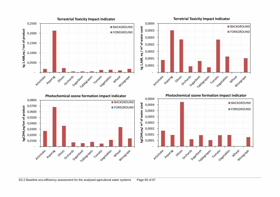
D2.2 Baseline eco-efficiency assessment for the analysed agricultural water systems Page 65 of 67
-
0,0500
0,1000
0,1500
0,2000
0,2500kg
1.4
dB
,eq
/ t
on
of
pro
du
ct
Terrestrial Toxicity Impact Indicator
BACKGROUND
FOREGROUND
-
0,0001
0,0001
0,0002
0,0002
0,0003
0,0003
0,0004
kg 1
,4d
B, e
q /
m³
of
wat
er
use
d
Terretrial Toxicity Impact Indicator
BACKGROUND
FOREGROUND
-
0,0100
0,0200
0,0300
0,0400
0,0500
0,0600
0,0700
0,0800
kgC
2H
4,e
q/t
on
of
pro
du
ct
Photochemical ozone formation impact indicator
BACKGROUND
FOREGROUND
-
0,0001
0,0001
0,0002
0,0002
0,0003
0,0003
0,0004
0,0004
kgC
2H
4,e
q/
m³
of
wat
er
use
d
Photochemical ozone formation impact indicator
BACKGROUND
FOREGROUND

D2.2 Baseline eco-efficiency assessment for the analysed agricultural water systems Page 66 of 67
-
0,0050
0,0100
0,0150
0,0200
0,0250
0,0300
0,0350
0,0400
0,0450
0,0500kg
Fe-e
q/t
on
of
pro
du
ct
Mineral Depletion Impact Indicator
BACKGROUND
FOREGROUND
-
0,0000
0,0000
0,0000
0,0000
0,0001
0,0001
0,0001
kgFe
-eq
/ m
³ o
f w
ate
r u
sed
Mineral Depletion Impact Indicator
BACKGROUND
FOREGROUND
-
5,0000
10,0000
15,0000
20,0000
25,0000
30,0000
35,0000
40,0000
45,0000
kg o
il e
q/t
on
of
pro
du
ct
Fossil Fuel Depletion Impact Indicator
BACKGROUND
FOREGROUND
-
0,0500
0,1000
0,1500
0,2000
0,2500
0,3000
kg o
il e
q /
m³
of
wat
er
use
d
Fossil Fuel Depletion Impact Indicator
BACKGROUND
FOREGROUND

D2.2 Baseline eco-efficiency assessment for the analysed agricultural water systems Page 67 of 67
-
20,0000
40,0000
60,0000
80,0000
100,0000
120,0000m
³ /
ton
of
pro
du
ct
Freshwater Depletion Impact Indicator
FOREGROUND