BANK OF REECE Workin EURg POSYSTEM aper · Our results control for household structure, degree of...
43
BANK OF GREECE EUROSYSTEM Working Paper Eirini Andriopoulou Apostolos Fasianos Athanassios Petralias Estimation of the adequate living expenses threshold during the Greek crisis 2 NGPAPERWORKINGPAPERWORKINGPAPERWORKINGPAPERWORKI MAY 2019 6 1
Transcript of BANK OF REECE Workin EURg POSYSTEM aper · Our results control for household structure, degree of...

BANK OF GREECE
EUROSYSTEM
Working Paper
Economic Research DepartmentSpec ia l S tud ies D iv i s ion21, E. Venizelos AvenueG R - 1 0 2 5 0 , A t h e n s
Tel.:+ 3 0 2 1 0 3 2 0 3 6 1 0Fax:+ 3 0 2 1 0 3 2 0 2 4 3 2w w w . b a n k o f g r e e c e . g r
BANK OF GREECE
EUROSYSTEM
WORKINGPAPERWORKINGPAPERWORKINGPAPERWORKINGPAPERISSN: 1109-6691
Eirini Andriopoulou Apostolos Fasianos
Athanassios Petralias
Estimation of the adequate living expenses threshold during the Greek crisis
2WORKINGPAPERWORKINGPAPERWORKINGPAPERWORKINGPAPERWORKINGPAPERMAY 2019
61
BANK OF GREECE Economic Analysis and Research Department – Special Studies Division 21, Ε. Venizelos Avenue GR-102 50 Athens Τel: +30210-320 3610 Fax: +30210-320 2432 www.bankofgreece.gr Printed in Athens, Greece at the Bank of Greece Printing Works. All rights reserved. Reproduction for educational and non-commercial purposes is permitted provided that the source is acknowledged. ISSN 1109-6691

ESTIMATION OF THE ADEQUATE LIVING EXPENSES THRESHOLD DURING THE GREEK CRISIS
Eirini Andriopoulou
Council of Economic Advisors, Ministry of Finance
Apostolos Fasianos Council of Economic Advisors, Ministry of Finance
Athanassios Petralias Bank of Greece
ABSTRACT The aim of this study is to present the underlying methodology behind the estimation of the Adequate Living Expenses (ALE) Threshold for the Greek population. The ALE threshold was first introduced in 2014 by the Greek authorities as a benchmark, mainly for protecting over-indebted mortgage holders from foreclosure of the primary residence. In this manuscript, we present alternative methodological approaches and specifications considered to estimate this threshold and we report updated estimates for the year 2017. The ALE threshold is defined through expenditure for the purchase of goods and services and interpreted as the income level that the household should possess in order to cover the level of acceptable living expenses, following the median expenditure pattern of Greek households. By taking into consideration the main categories of the Greek Household Budget Survey, we examined different expenditure specifications, based on the necessity of the needs covered by gradually excluding items that could be considered as “luxury” items (four scenarios were developed). Quantile regression and linear robust regression accounting for the presence of outliers was applied and various model specifications were tested. Our results control for household structure, degree of urbanization and mortgage holding, and interactions among them. In 2017, for a family with two children ALE threshold ranged from 1,196€ to 1,497€ per month, reduced by approximately 11.5% compared to 2012, depending on the expenditure specification. The estimated ALE threshold lies considerably above the poverty line in all cases. Keywords: Mortgage, household budget, insolvency, reference budget, foreclosures. JEL Classification: G18, G21 Acknowledgments: The Adequate Living Expenses threshold in Greece was first estimated in 2014, based on 2012 Household Budget Survey data, by a team consisting of Eirini Andriopoulou, Athanassios Petralias and Ioannis Vintzilaios, under the auspices of the Council of Economic Advisors of the Ministry of Finance and the General Consumers Secretariat of the Ministry for Development and Competitiveness. We are thankful to Chrysa Leventi, De Wilde Marjolijn, Tess Penne, and the participants of the Council of Economic Advisors research seminar in March 2019 for their useful comments. The methodology applied was agreed with the IMF, ECB and European Commission, in the framework of the second economic adjustment programme and was officially approved by the Governmental Council of Private Debt Management. All the remaining errors are the responsibility of the authors. The views expressed in the article are those of the authors and should not be attributed neither to the Council of Economic Advisors nor to the Bank of Greece or the Eurosystem.
Correspondence: Athanasios Petralias Department of Statistics Bank of Greece 21 El. Venizelos Av., 10250 Athens, Greece Email: [email protected]
3
1. Introduction
The Adequate Living Expenses (ALE) threshold, originally introduced in 2014, is used
by the Greek authorities as a benchmark for protecting mortgage-holders from foreclosure
of the primary residence. The threshold also serves as a guideline for courts and judiciary on
the application of the legislated home protection schemes1 on household insolvency, as well
as for the out-of-court loan restructuring procedure by the banking sector. The aim of this
study is (a) to present the methodology for the estimation of the Adequate Living Expenses
(ALE) threshold, (b) to update the 2012 estimates to the most recent ones, and, (c) to
present alternative methods that can be used to update these estimates on an annual basis.
Periodic updates of the ALE threshold are necessary in the light of changes in the
prices of the consumer basket, consumer habits, and household incomes. Furthermore,
given that the ALE threshold is a key parameter for the non-performing loans resolution, as
the level of ALE and its policy applications (protection of primary residence from foreclosure,
state-subsidy to mortgage holders etc.) may affect mortgage-holders behavior itself, it is
crucial to investigate the sensitivity of the ALE threshold results to alternative methods and
suggest possible improvements.
According to the IMF/EC/ECB Guidance on Household Debt Definitions (12/05/2013) a
definition of acceptable living expenses safeguards “a minimum standard of living so as to
protect debtors while facilitating creditors in recovering all, or at least a portion of the debts
due to them. One of the strengths of using consensual budget standards is the level of
transparency it affords in the debt resolution process. It ensures that debtors, creditors and
any third-parties involved can recognize a repayment schedule as being fair and thus
provides the confidence for all parties to expeditiously agree on new lean terms”.
Broadly, ALE is related to the notion of reference budgets. According to the European
Consumer Debt Network (ECDN, 2009), “reference budgets are expenditure patterns for
different types of households. Based on the household composition (number of members,
age), the disposable income and some other characteristics (like housing situation,
possession of a car, special needs of members), an expenditure pattern is given that suits the
situation of the household. Reference budgets can be based on empirical data (e.g. budget
enquiries) or constructed by budget experts.” On policy grounds, reference budgets and ALE
thresholds are used for multiple purposes including the estimation of an adequate standard
1 In particular, laws 3869/2010, 4161/2013, 4346/2015 and 4549/2018, govern the protection scheme
for primary residence in Greece.

4
of living, estimation of additional income support bellow the guaranteed minimum income2,
debt rescheduling, financial education, the calculation of alternative credit scores,
measuring the extent of poverty and assessing the adequacy of minimum wages and social
benefits (Goedemé et al., 2015; Storms et al., 2014).
There exists a variety of approaches on developing reference budgets (Citro and
Michael 1995), but two are predominant in the relevant literature. The first approach,
followed in this analysis, is to rely on empirical data and household surveys. Within
European countries, Denmark, Germany, Greece, and Latvia follow this approach. Another
methodological approach (used in the case of Ireland (ISI, 2013) and other countries) is to
form task groups of experts (i.e. nutrition scientists etc.), so as to synthesize baskets of
goods and services, a household is “reasonable” to consume, and evaluate their cost on a
continuous basis according to the CPI index.
According to a review of reference budgets in Europe, conducted by Storms et al.
(2014), 23 EU countries have constructed reference budgets in the past four decades that
are still being used.3 Out of the 61 reference budgets studied (some countries have
developed more than one in the past), 47 make use of expert knowledge, 41 use household
budgets survey (HBS) data, 22 focus groups decisions, 22 international and regional
guidelines, 15 survey data besides HBS and 3 market research; several countries combine
more than one data sources such as expert knowledge and focus groups decisions.
The adequate living expenses threshold in this study is estimated through the
reported household expenditure for the consumption of selected baskets of goods and
services and is interpreted as the income level that the household should possess in an
annual basis in order to be able to cover the level of acceptable living expenses. The data of
Greek Household Budget Survey (HBS) of the Hellenic Statistical Authority (ELSTAT) are used
for the estimation of the threshold.
It is tricky to determine what is “reasonable” or “adequate” when it comes to
expenditure or income and one should always try to minimize the risk of subjective
assumptions. The main idea in our approach is to propose a “statistically reasonable”
definition, by studying the observed household expenditures and try to estimate how much
2 See, for example, a recent study by Penne et al (2019), who propose reference budgets as an EU
policy indicator to assess adequacy of minimum incomes and illustrate this with the case of Belgium. 3 Notable examples include: Collins et al. (2012); Hoff et al. (2010); Kemmetmüller and Leitner (2009);
Konsument Verket (2009); Preuße (2012). A detailed list of publications outlining relevant work on reference budgets by country can be found here: https://www.referencebudgets.eu/copy-of-publications.

5
the median Greek household actually spends, after excluding non-prior and luxury expenses.
With respect to non-prior expenses we present four different specifications of them, having
in mind that adequate expenses should allow each person to receive nutritionally adequate
food, have descent clothing, cover daily transportation costs, have access to education and
health and be an active member in the society.
The rest of the manuscript proceeds as follows. The second section presents the
datasets used, the third section the methodology applied and the fourth section the results
of the econometric estimation, including a comparative analysis of the different techniques
to update ALE, a comparison with poverty thresholds and a sensitivity analysis when
applying the suggested methodology for the whole 2010-2017 period. The fifth section
concludes.
2. Data
The estimates of the ALE threshold are based on the micro-data of the Greek
Household Budget Survey (HBS) of the Hellenic Statistical Authority (ELSTAT) (see Hellenic
Statistical Authority, 2018). HBS is a national survey collecting information from a
representative sample of households, on households’ composition, members’ employment
status, living conditions and, mainly, focusing on their members’ expenditure on goods and
services. The expenditure information collected from households is very detailed.
Specifically, information is collected on the basis of total expenditure categories like "food",
‘'clothing - footwear', "health ", etc., but also separately for each expenditure, for example,
white bread, fresh whole milk, fresh beef etc., footwear for men, footwear for women etc.,
services of medical analysis laboratories, pharmaceutical products etc.
The main purpose of the HBS is to determine in detail the household expenditure
pattern in order to revise the Consumer Price Index. Moreover, HBS is the most appropriate
source in order to (a) complete the available statistical data for the estimation of the total
private consumption, (b) study the households’ expenditures and their structure in relation
with other economic, social and demographic characteristics, (c) analyze the changes in the
living conditions the households in comparison with as previous surveys, (d) study the
relation between households purchases and receipts in kind, and (e) study the changes in
the nutritional habits of the households of the country.
From 2008 it was decided, the Greek HBS survey should be annual and consistent,
6
namely has duration one year and takes place every year. In the framework of the current
analysis we analyzed the data of HBS’s of the years 2010 up to 2017. For the period 2010-
2013, the sample size is approximately 8,500 individuals and 3,500 households. From 2014
onwards the sample size has increased to approximately 14,500 individuals and 6,000
households. The sample is adjusted so as to resemble the distribution of the total
population, using ELSTAT’s HBS sampling weights. Various variables of the HBS were used for
the current analysis as described in detail below.
The second dataset used is the monthly sub-indices, sub-groups and items of the
Consumer Price Index (CPI) published by ELSTAT, along with the corresponding CPI weights.
These data are used to examine an alternative method to update ALE thresholds on an
annual basis, when only price changes are taken into account.
The third dataset, used for comparative purposes, is the European Union Statistics on
Income and Living Conditions (EU-SILC) database. EU-SILC is a cross-sectional and
longitudinal sample survey, coordinated by Eurostat, based on data from the EU member
states. EU-SILC provides data on income, poverty, social exclusion and living conditions in
the European Union. EU-SILC micro data is gathered by the member states of the European
Union and collated by Eurostat. There are two data types: Cross-sectional data pertaining to
fixed time periods, with variables on income, poverty, social exclusion and living conditions,
and longitudinal data pertaining to individual-level changes over time, observed periodically,
usually over four years. Social exclusion and housing-condition information is collected at
household level. Income at a detailed component level is collected at personal level,
with some components included in the 'Household' section. Labour, education and
health observations only apply to persons aged 16 and over. EU-SILC was established to
provide data on structural indicators of social cohesion (at-risk-of-poverty rate, S80/S20 and
gender pay gap) and to provide relevant data for the two 'open methods of coordination' in
the field of social inclusion and pensions in Europe. The 2012 and 2017 EU-SILC data are
used, so as to compare ALE thresholds for different household synthesis with the poverty
thresholds derived on basis of the EU-SILC survey.
3. Methodology
The applied methodology involves quantile and robust linear regression of total
consumption expenditure as formed after the exclusion of certain expenses, according to
the household type such as single household, household with two adults, number of
7
children, number of extra adults, mortgage holding and urbanization. Different versions of
the expenditure variable, as well as different model specifications have been tested. In the
following paragraphs, we describe the methodology in detail: (a) the construction of the
dependent variable, (b) the construction of independent variables, (c) the model
specifications and estimation techniques and (d) the strategies used to update ALE
thresholds on an annual basis.
3.1 Expenditure variable
The current study seeks to determine an adequate level of expenditure for each type
of household, translated as an adequate level of income sources that the household should
possess in order to be able to reach the adequate living expenses threshold. Therefore,
expenditure is the main variable to be defined. Using the HBS data, we have chosen to
exclude (under different exclusion scenarios) from the already calculated total household
expenditure variable of the Greek Household Budget Survey certain expenses which are
considered to be non-prior or luxury. We took into consideration all the main categories
included in the HBS: Food and non-alcoholic beverages, alcoholic beverages and tobacco,
clothing and footwear, housing, water, electricity, gas and other fuels, furnishings,
household equipment and routine maintenance of the house, health, transport,
communications, recreation and culture, education, restaurants and hotels, miscellaneous
goods and services.
The rational is that in order to provide alleviation to people in dire economic situation,
reasonable cost of living should cover basic needs of descent living. We take into account
expenses related to social services provided by the state (i.e. national health system, public
schools, public transportation etc.) and we exclude additional or alternative options
provided by private sector. Thus, the approach is focused on objective needs of households
and not on personal wishes or demands.
Based on the above rational, four different definitions of the expenditure variable
have been used for testing the sensitivity of the results, formed by gradually excluding the
following groups of expenses: The analytical HBS categories excluded from each expenditure
specification are provided in Table 1. In the 1st group of variables excluded are expenses
related to rents, private health, private education, private insurance and luxury; in the 2nd
group of variables excluded are additional expenses related to travelling, hobbies, alcohol,
tobacco and hotel expenses, except pets and veterinary services; in the 3rd group of variables
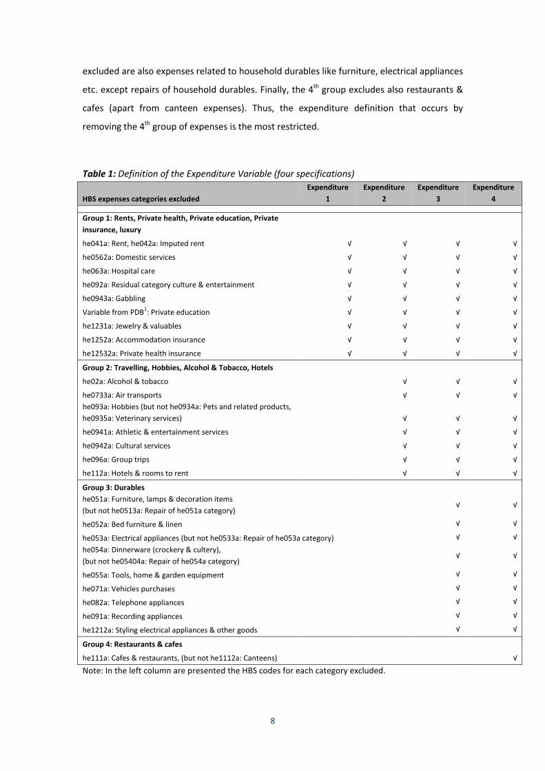
8
excluded are also expenses related to household durables like furniture, electrical appliances
etc. except repairs of household durables. Finally, the 4th group excludes also restaurants &
cafes (apart from canteen expenses). Thus, the expenditure definition that occurs by
removing the 4th group of expenses is the most restricted.
Table 1: Definition of the Expenditure Variable (four specifications)
HBS expenses categories excluded
Expenditure
1
Expenditure
2
Expenditure
3
Expenditure
4
Group 1: Rents, Private health, Private education, Private
insurance, luxury
he041a: Rent, he042a: Imputed rent √ √ √ √
he0562a: Domestic services √ √ √ √
he063a: Hospital care √ √ √ √
he092a: Residual category culture & entertainment √ √ √ √
he0943a: Gabbling √ √ √ √
Variable from PDB1: Private education √ √ √ √
he1231a: Jewelry & valuables √ √ √ √
he1252a: Accommodation insurance √ √ √ √
he12532a: Private health insurance √ √ √ √
Group 2: Travelling, Hobbies, Alcohol & Tobacco, Hotels
he02a: Alcohol & tobacco
√ √ √
he0733a: Air transports
√ √ √
he093a: Hobbies (but not he0934a: Pets and related products,
he0935a: Veterinary services) √ √ √
he0941a: Athletic & entertainment services √ √ √
he0942a: Cultural services √ √ √
he096a: Group trips
√ √ √
he112a: Hotels & rooms to rent √ √ √
Group 3: Durables
he051a: Furniture, lamps & decoration items
(but not he0513a: Repair of he051a category) √ √
he052a: Bed furniture & linen √ √
he053a: Electrical appliances (but not he0533a: Repair of he053a category) √ √
he054a: Dinnerware (crockery & cultery),
(but not he05404a: Repair of he054a category) √ √
he055a: Tools, home & garden equipment √ √
he071a: Vehicles purchases
√ √
he082a: Telephone appliances √ √
he091a: Recording appliances √ √
he1212a: Styling electrical appliances & other goods √ √
Group 4: Restaurants & cafes
he111a: Cafes & restaurants, (but not he1112a: Canteens) √
Note: In the left column are presented the HBS codes for each category excluded.
9
In total, we consider Expenditure 3 to be the version that contains all the necessities
that the households must have the ability to consume in order to be able to achieve an
adequate standard of living, including only one type of entertainment for household
members “Cafes and restaurants”. In specification 4, the “Cafes and restaurants” (excluding
canteens) expenditure has also been removed. In this report, we present the descriptive
statistics for the four different definitions of the dependent variable and the regression
results for three main alternative model specifications under each version of the
expenditure variable.
The definition of expenditure used in the current analysis does not include any kind of
imputed expenditure (e.g. from self-production). Moreover, it does not include any
expenses for loan installments/arrears and rent or payment of taxes and levies. In this way,
the thresholds of adequate living expenses are defined without housing financing costs.
Subsequently, an amount for loan repayment can be calculated proportionally to the
difference of net household income (after subtracting direct taxes and social security
contributions paid4) and ALE of each household.
3.2 Factors differentiating household expenditure
The selection of the independent variables was based on scientific criteria on what
determinants could affect the expenditure level of a household and on the final need to
produce clear, straightforward and coherent guidelines for banks and borrowers. Thus,
despite the fact that the exercise could be developed using more potential regressors (i.e.
participants’ educational level, age, gender, employment status, branch of economic
activity, nationality etc.), we had to keep it simple so that the final ALE estimation can be
calculated using objective household standards (like the household synthesis) that are
acceptable from a legal and policy making perspective. Certainly, from an academic
perspective, multiple regressors with regards to the socioeconomic status of the household
could be examined in order to identify different patterns of consumption habits, and how
the level of consumption differs as these characteristics change.
Table 2 presents the regressors considered which can be grouped into three
categories: (a) household synthesis, (b) regressors capturing potential differentiated
4 In terms of the actual implementation of the scheme, it should be taken into account that taxes paid
may differ from assessed taxes. Thus, it is important to ensure that the taxes that are subtracted during the judgement for the payment capacity of households have actually been paid. To this end, assessment based only on tax-returns clearance is not enough.
10
behavior of mortgage holders and (c) regressors capturing the level of urbanization of the
household residence.
Table 2: Independent Variables
Independent Variables
Variable Name Variable Label
A. Household (hh) synthesis
dummy_one_adult One adult in the hh
dummy_twoplus_adults At least two adults in the hh
num_add_adults Number of additional adults in hh >2
num_dep_children Number of dependent children in hh
B.Mortgage holding effect
dummy_mortgage Mortgage holding (1: mortgage, 0: home ownership/free-leasing/rent)
int_num_dep_children_mortgage Interaction number of dependent children with mortgage holding
int_twoplus_adults_mortgage Interaction at least two adults with mortgage holding
int_num_add_adults_mortgage Interaction number of additional adults with mortgage holding
C.Urbanization effect
dummy_urban Urban areas
dummy_semi_urban Semi-urban_areas
dummy_agr Agricultural_areas
int_num_dep_children_agr Interaction number of dependent children with agriculture
int_twoplus_adults_agr Interaction at least two adults with agriculture
int_num_add_adults_agr Interaction number of additional adults with agriculture
The main variable used in terms of policy to differentiate the ALE threshold is the
household synthesis. By testing various specifications, we have concluded that the best way
is to use as baseline group the single adult household type, introduce a dummy to capture
the existence of second adult in the household and then introduce linearly the number of
additional adults, since there is limited number of observations for households with three or
more dependent adults in HBS. It is important to note that the additional adults in a
household may or may not have a personal taxable income. However, they consume and
raise the expenditures of a household. Thus, we propose in practice, when comparing the
taxable income of the debtor to the households’ adequate living expenses, to use the ALE of
additional adults only in the case they are considered as dependent individuals to the debtor
by the tax office.
With regards to the children, we used the number of children linearly, since there was
a limited number of observations with four or more children in the sample, while such a
solution would be in favor of families with one child as opposed to families with more
children, which might be an awkward result from a social policy point of view. It must be
noted that we have also tested various age groups for distinguishing dependent children
11
categories. However, the sample size is a limitation for pursuing properly this exercise,
while this division also complicates the formula for the calculation of ALE for each family
type and demands frequent updates following the growing-up of children, which might not
be convenient for a long-term rescheduling of loan repayments and is costly from an
administrative point of view. For the needs of the ALE estimation dependent children are
defined as individuals aged 0-17 years old, or individuals aged 18-24 who are economically
inactive (students, soldiers, those with disabilities) and reside in the same household.
Mortgage holding of primary residence5 is introduced as a dummy in the regression
taking the value of `1’ if the household holds a mortgage for the primary residence and ‘0’
for home-ownership, free-leasing or rent of the primary residence. Interactions of the
mortgage holding dummy with the household synthesis variables are considered so as to
capture differentiated behaviors of mortgage holders in different household types.
For the construction of the urbanization dummies the HBS coding of regions into
urban, semi-urban and rural areas was used. It must be noted that we have also tested
additional specifications based on the NUTS 1 division of regions (Northern Greece, Central
Greece, Attica, Aegean islands and Crete). However, the size of the sample did not permit to
estimate more detailed regional divisions and the results based on this categorization cannot
replicate the high heterogeneity within these regions. Thus, considering the data availability
and that the division on basis of NUTS 1 codes is rather general and based solely on
administrative criteria, we propose as a more robust scenario to divide areas among
urban/semi-urban and agricultural.
It has to be noted that from the variables presented above, in the practical application
of ALE threshold only the household synthesis variable is used. As already mentioned, the
inclusion of any additional characteristic (e.g. diversification between urban and rural areas)
may be considered as discreet treatment, which is not acceptable from a legal and political
perspective. For example, if a lower threshold is estimated for agricultural regions then
those living in cities may have more beneficial terms in their loan restructuring. Also having
different thresholds for those holding a mortgage than those who don’t (taking into account
that loan payments and rents are exempted from all expenses specifications) can lead to
unfair situations when ALE thresholds are used in political courts and judiciary in general.
Moreover, we have not included a dummy to capture the existence of disable or
5 The mortgage holding indicator concerns only housing loans and no other loans that might have as
collateral the first residence.
12
chronic ill individuals in the household, because this should be assessed on a case by case
basis by financial institutions, either for loan repayment or for not starting a home-
foreclosure process, irrespectively of the consumption/ expenditure patterns of these
households.
3.3 Model specifications and estimation methods
Given the definitions of dependent and independent variables, we have estimated
three model specifications: Specification A including only the household synthesis variables
(A in Table 2), Specification B including the household synthesis and mortgage holding effect
variables (A & B in Table 2) and Specification C including the household synthesis and
urbanization effect variables (A & C in Table 2).
Note that with respect to household synthesis one adult in the household is kept as a
reference category (i.e. is not included in the regression) and with respect to urbanization
effect the reference category includes both urban and semi-urban areas, since the sample
was more limited in semi-urban areas and significant differentiation was mainly observed in
agricultural areas.
One of the main methodological issues when analyzing expenditure (or income) data
is the presence of outliers and the right-skewness of the distribution (see Figure 1). That is,
there are relatively few individuals with rather high expenses. This causes the estimates of
the average expenditure to be significantly higher than the median and thus not
representable of the consumption patterns of a typical household. We employ two
alternative econometric techniques to cope with this issue: (a) linear robust regression in
which standardized residuals with large absolute values (i.e. >2) are omitted from a second
step robust regression and (b) quantile regression which seeks to estimate the median
expenditure.
In all cases we employ a linear model of the form
𝑦 = Χ𝜃 + ε,
where 𝑦 is the (𝑛 × 1) vector containing one of the four alternative specifications for
expenditure variable, 𝛸 the (𝑛 × 𝑝) matrix containing the independent variables under
specification A, B or C above, 𝜃 the (𝑝 × 1) vector with the unknown regression parameters
to estimate and ε the (𝑛 × 1) vector with the error terms. In total, we estimate for the HBS
data of a given year 24 regressions (3 sets of independent variables with 4 different
13
specifications of the dependent variable, using either linear robust regression or quantile
regression).
Robust linear regression (see Huber, 1964, 1981; Rousseeuw & Leroy, 1987) is a
common method used to perform linear regression in the presence of outliers and
heteroscedasticity. This involves an iterative reweighted least squares algorithm that
minimizes the standardized residuals, which are multiplied with a loss function associated
with Cook’s distance. However, the robust linear regression has been reported efficient
when there exist isolated outliers. In the presence of clusters of outliers the method does
not guarantee to identify all leverage points (Rousseeuw and Van Zomeren, 1990).
Keeping in mind that we want to identify a reasonable level of expenses, so that
resembles the expenses of a “typical” household, we are mainly interested with the main
mass of the expenditure distribution, where most of households lie. Thus, omitting clusters
of outliers that lie in the tails of the distribution is not in contrast with the purposes of this
analysis.
Consequently, in order to reduce the probability the robust linear regression
estimates to be affected by clusters of outliers we remove cases the absolute standardized
residuals take values above 2, corresponding to approximately 5% of observations, and re-
run the robust linear regression (for a description of similar techniques see Ben-Gal, 2005).
The second method employed is quantile regression (see Koenker, 2005). Under this
method, median regression estimates are obtained, conditional on the values of the
independent variable, which are not affected by outliers. One of the drawbacks of quantile
regression is that the estimated conditional quantiles are empirical, so they could be
affected easily by small size samples in each category of the independent variables. To our
best knowledge, it is the first time that a consumer basket for different household types,
estimated with the quantile regression method, has been applied to an analysis of reference
budgets. Yet, quantile regressions has been found useful on obtaining robust estimates on
poverty analysis, a literature that is very close to our focus in the present study (see, for
example, Muller (2002), Muller and Bibi (2010), Brück et al (2010)).
One appealing characteristic of the model specification is its simplicity, which is
desirable for policy implementation purposes. So under Specification A, by holding the
variable “dummy_one_adult” as the reference level, the estimated constant of the
regression is actually the ALE threshold for one adult. Then, by adding the coefficient of the
variable “dummy_twoplus_adults” the ALE threshold for a two adult household is
14
calculated. By adding two times the coefficient of the variable “num_dep_children” we
obtain the ALE thresholds for a family with two children. Similarly, one can add additional
adults or children. In this way, since ALE are derived directly by the actual regression
coefficients, the calculation is completely transparent and any update with new waves of the
HBS straightforward.
3.4 Annual updates of the ALE thresholds
On basis of the above, one way to update annually the ALE thresholds is to re-run the
model(s) based on either robust linear regression or quantile regression, on basis of the
latest HBS data, which is the proposed strategy followed in this manuscript.
However using as a basis older HBS data could provide an alternate estimate of
adequate living expenses, especially when there is rapid decline or increase in real incomes,
which is not accompanied by an analogous change of prices. Anchored methods (keeping
still the base period) to determine certain thresholds (i.e. poverty line) can prove robust
during rapid recession or rapid development periods.
In such cases, one can use the ALE thresholds of a base period and update the
thresholds taking into account the changes in CPI categories. As an exercise we updated ALE
thresholds up to 2017 on basis of this method, taking the 2012 published ALE thresholds as
baseline. More specifically, for each expenditure specification (see Table 1) and year, we
constructed the corresponding re-weighted CPI index, taking into account the sub-groups
and items in the expenditure specification, on basis of ELSTAT’s CPI data and weights. Then,
the 2012 ALE thresholds increased or decreased inter-temporally according to evolution of
the re-weighted CPI index.
This method has the property that the reported ALE thresholds are not affected by
changes in income or consumer behaviors, but only from changes in prices. This is equal to
estimating at a particular point in time a specific basket of goods (according to the
consumption habits of this period) and keeping it constant through a time. For periods of
recession, it might be more appropriate because specific household types may be more
financially constrained than others and then squeeze more their consumption. Thus, the
changes in expenditures might not reflect changes in necessities or consumption patterns,
but changes in liquidity for different household types. This method can be used as an
alternative short-term strategy to update the ALE thresholds, especially in periods of rapid
income changes, but is not appropriate for long-term use, since it does not capture changes
15
in consumer consumption patterns.
4. Results
4.1 Descriptive statistics
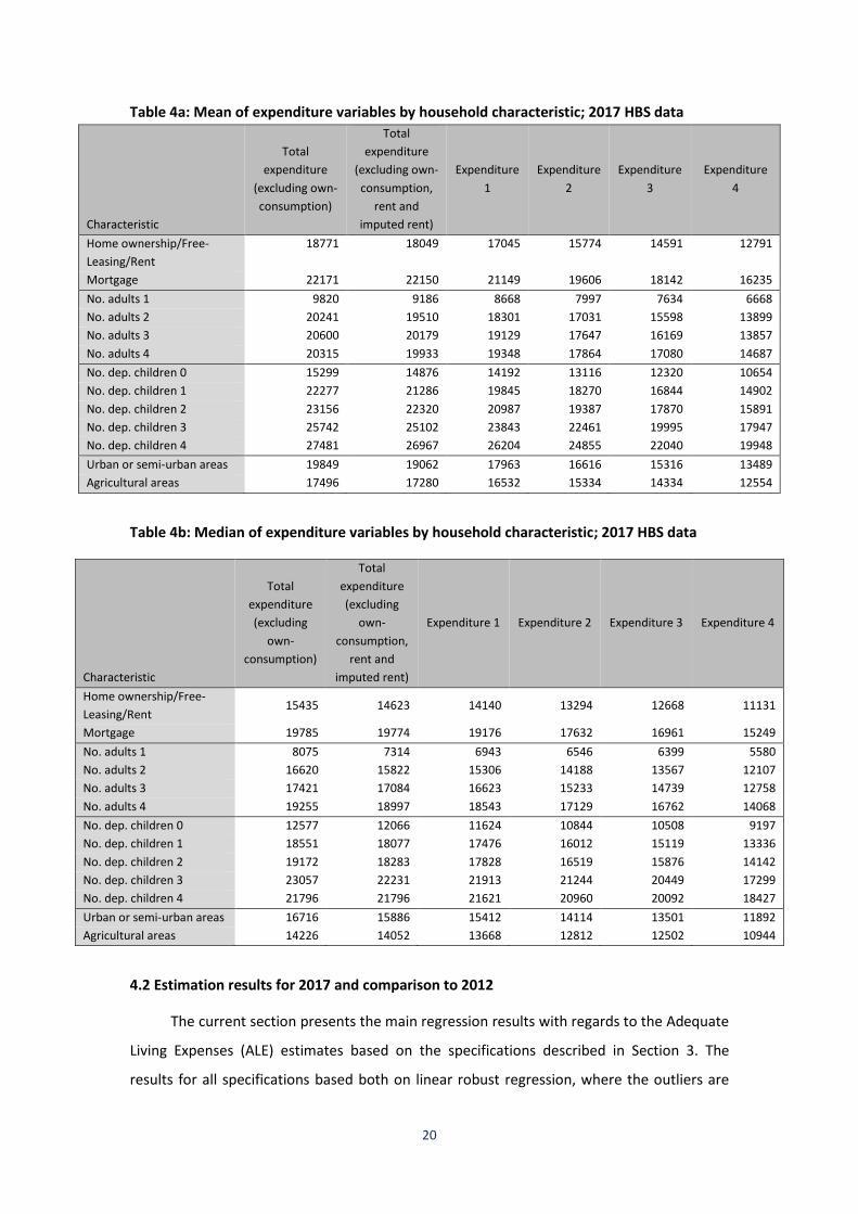
In Table 3a is presented the distribution of the four definitions of expenditure on basis
of the 2012 HBS data and in Table 3b, on basis of the 2017 data. In Tables 4a and 4b, the
distribution of the four expenditure variables for the year 2017 is presented according to the
household composition (number of adults and number of dependent children), the
mortgage holding variable, and the urbanization.
As indicated by the difference among the mean and median of the expenditure
variables (see Tables 3a, 3b and Figure 1) the distribution is right-skewed with the presence
of outliers, i.e. there exist few observations with relatively high values. For this purpose in
the regression analysis we adjust for the presence of outliers, using alternative inference
techniques.
According to the descriptive results of our analysis using the Household Budget Survey
(HBS) data:
The average (median) total household expenditure amounted to 21,796€ (17,263€)
per year in 2012 and 19,210€ (15,986€) per year in 2017, down by 11.9% (7.4%).
The average (median) total household expenditure if we remove rent and imputed
rent amounted to 21,065€ (16,552€) per year in 2012 and 18,578€ (15,420€) per
year in 2017, down by 11.8% (6.8%).
The average (median) household expenditure excluding the 1st group of expenses
(rents, private health, private education, private insurance, luxury) amounted to
19,960€ (16,101€) per year in 2012 and 17,574€ (14,967€) per year in 2017, down by
11.9% (7.0%). Note that for households below the 30% percentile, Expenditure 1
approximates the total expenditure if we remove only rent, signaling that these
households indeed consume very less of the other types of goods and services
included in the 1st group (such as private education, private health and luxury).
The average (median) household expenditure excluding the 1st group and 2nd group
of expenses (travelling, hobbies, alcohol & tobacco, hotels) amounted to 18,410€
(14,913€) per year in 2012 and 16,268€ (13,785€) per year in 2017, down by 11.6%
(7.6%).
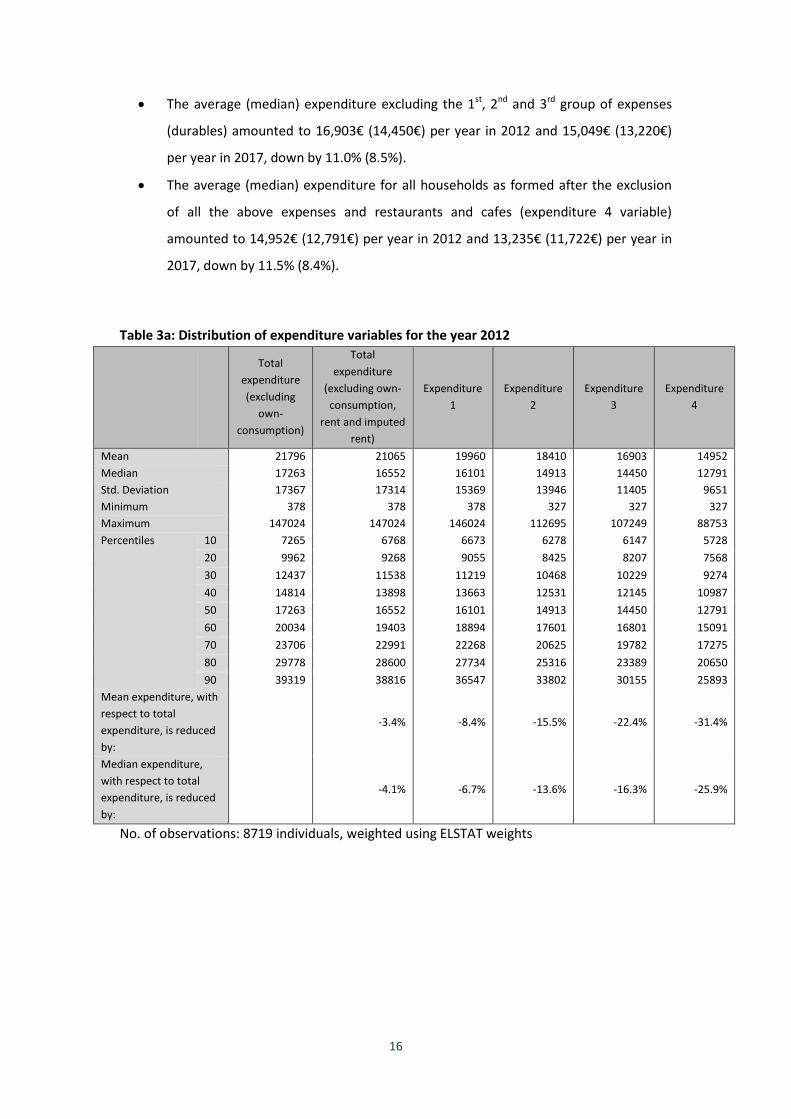
16
The average (median) expenditure excluding the 1st, 2nd and 3rd group of expenses
(durables) amounted to 16,903€ (14,450€) per year in 2012 and 15,049€ (13,220€)
per year in 2017, down by 11.0% (8.5%).
The average (median) expenditure for all households as formed after the exclusion
of all the above expenses and restaurants and cafes (expenditure 4 variable)
amounted to 14,952€ (12,791€) per year in 2012 and 13,235€ (11,722€) per year in
2017, down by 11.5% (8.4%).
Table 3a: Distribution of expenditure variables for the year 2012
Total
expenditure
(excluding
own-
consumption)
Total
expenditure
(excluding own-
consumption,
rent and imputed
rent)
Expenditure
1
Expenditure
2
Expenditure
3
Expenditure
4
Mean 21796 21065 19960 18410 16903 14952
Median 17263 16552 16101 14913 14450 12791
Std. Deviation 17367 17314 15369 13946 11405 9651
Minimum 378 378 378 327 327 327
Maximum 147024 147024 146024 112695 107249 88753
Percentiles 10 7265 6768 6673 6278 6147 5728
20 9962 9268 9055 8425 8207 7568
30 12437 11538 11219 10468 10229 9274
40 14814 13898 13663 12531 12145 10987
50 17263 16552 16101 14913 14450 12791
60 20034 19403 18894 17601 16801 15091
70 23706 22991 22268 20625 19782 17275
80 29778 28600 27734 25316 23389 20650
90 39319 38816 36547 33802 30155 25893
Mean expenditure, with
respect to total
expenditure, is reduced
by:
-3.4% -8.4% -15.5% -22.4% -31.4%
Median expenditure,
with respect to total
expenditure, is reduced
by:
-4.1% -6.7% -13.6% -16.3% -25.9%
No. of observations: 8719 individuals, weighted using ELSTAT weights

17
Table 3b: Distribution of expenditure variables for the year 2017
Total
expenditure
(excluding
own-
consumption)
Total
expenditure
(excluding own-
consumption,
rent and imputed
rent)
Expenditure
1
Expenditure
2
Expenditure
3
Expenditure
4
Mean 19210 18578 17574 16268 15049 13236
Median 15986 15420 14967 13785 13220 11722
Std. Deviation 14388 14182 12264 11105 9056 7773
Minimum 26 26 26 26 26 0
Maximum 204325 185125 126471 107106 85094 70178
Percentiles 10 6819 6390 6237 5802 5681 5190
20 9210 8653 8495 8018 7791 7010
30 11453 10812 10486 9956 9597 8605
40 13608 13031 12619 11848 11301 10025
50 15986 15420 14967 13785 13220 11722
60 18514 17988 17487 16206 15304 13406
70 21711 21039 20371 19000 17815 15710
80 25693 24802 24118 22549 21124 18427
90 34206 32471 30509 28628 26121 22770
Mean expenditure, with
respect to total
expenditure, is reduced
by:
-3.3% -8.5% -15.3% -21.7% -31.1%
Median expenditure,
with respect to total
expenditure, is reduced
by:
-3.5% -6.4% -13.8% -17.3% -26.7%
No. of observations: 14457 individuals, weighted using ELSTAT weights.
Figure 1: Histograms of expenditure variables for the year 2017
18
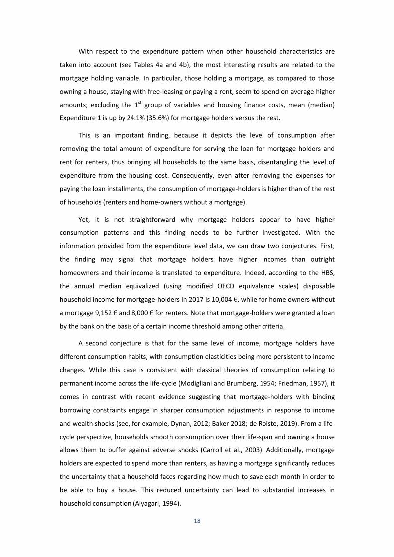
With respect to the expenditure pattern when other household characteristics are
taken into account (see Tables 4a and 4b), the most interesting results are related to the
mortgage holding variable. In particular, those holding a mortgage, as compared to those
owning a house, staying with free-leasing or paying a rent, seem to spend on average higher
amounts; excluding the 1st group of variables and housing finance costs, mean (median)
Expenditure 1 is up by 24.1% (35.6%) for mortgage holders versus the rest.
This is an important finding, because it depicts the level of consumption after
removing the total amount of expenditure for serving the loan for mortgage holders and
rent for renters, thus bringing all households to the same basis, disentangling the level of
expenditure from the housing cost. Consequently, even after removing the expenses for
paying the loan installments, the consumption of mortgage-holders is higher than of the rest
of households (renters and home-owners without a mortgage).
Yet, it is not straightforward why mortgage holders appear to have higher
consumption patterns and this finding needs to be further investigated. With the
information provided from the expenditure level data, we can draw two conjectures. First,
the finding may signal that mortgage holders have higher incomes than outright
homeowners and their income is translated to expenditure. Indeed, according to the HBS,
the annual median equivalized (using modified OECD equivalence scales) disposable
household income for mortgage-holders in 2017 is 10,004 €, while for home owners without
a mortgage 9,152 € and 8,000 € for renters. Note that mortgage-holders were granted a loan
by the bank on the basis of a certain income threshold among other criteria.
A second conjecture is that for the same level of income, mortgage holders have
different consumption habits, with consumption elasticities being more persistent to income
changes. While this case is consistent with classical theories of consumption relating to
permanent income across the life-cycle (Modigliani and Brumberg, 1954; Friedman, 1957), it
comes in contrast with recent evidence suggesting that mortgage-holders with binding
borrowing constraints engage in sharper consumption adjustments in response to income
and wealth shocks (see, for example, Dynan, 2012; Baker 2018; de Roiste, 2019). From a life-
cycle perspective, households smooth consumption over their life-span and owning a house
allows them to buffer against adverse shocks (Carroll et al., 2003). Additionally, mortgage
holders are expected to spend more than renters, as having a mortgage significantly reduces
the uncertainty that a household faces regarding how much to save each month in order to
be able to buy a house. This reduced uncertainty can lead to substantial increases in
household consumption (Aiyagari, 1994).

19
This puzzle deserves further investigation, as it might reveal the large presence of
strategic defaulters on non-performing loans (NPLs) 6, as well as the high re-default
probability of these borrowers after a loan restructuring. If this is the case, the policy
implication for NPLs is that restructuring and protection schemes should ensure that the
thresholds set do not allow the non-performing borrowers to continue an “excessive
consumption” habit compared to the rest of the population, but to direct this extra
expenditure to the repayment of the loan.
As it concerns the regressors related to household composition the results are as
expected. Generally, the higher number of adults, the higher the expenses. A large
difference is observed among one and two adults (expenses more than double), whereas the
additional expenses for extra adults in the household are relatively small, reflecting higher
economies of scale7. We observe also a large difference in expenditure when moving from
zero to one child and a smaller difference when moving from one to two children, reflecting
much larger economies of scale in the subsequent children. However, the median
expenditures for families with four children are lower or comparable to families with three
children. This can be attributed to the sociodemographic characteristics of families with
many children, as well as to the relatively small sample size of households with a high
number of children.
Total expenditure is higher in urban and semi-urban areas compared to agricultural
areas, by 13.45% on average or 4.57% on basis of the median. However, it is interesting to
note that for more conservative specifications, such as Expenditure 3 and Expenditure 4 the
median expenditure does not differ considerably on basis of urbanization. This indicates that
some of the “luxury” items that are included in specifications 1 and 2 are consumed to a
much lesser extent in rural than urban areas.
6 According to an analysis performed by the Council of Economic Advisors, using administrative data
from tax returns and information from the Hellenic Bank Association, the number of non-performing borrowers holding a mortgage loan in December of 2018 was 148,650 over 588,530 borrowers (25%), holding a total debt of 14.7 billion € over 43.9 billion € of mortgage loans (33%). 7 Αn interpretation regarding very low economies of scale in households with one and two adults may
relate to the age profile of the household. We estimated the mean consumption controlling for age of household residents, and indeed the economies of scale are more evident in older ages. For example, for 2017, the total consumption of households below 60 years of age increases by 68% as we move from the first to the second adult. The corresponding increase for those 60 and over is above 90%. This heterogeneity may reveal different consumption patterns across households of different ages.
20
Table 4a: Mean of expenditure variables by household characteristic; 2017 HBS data
Characteristic
Total
expenditure
(excluding own-
consumption)
Total
expenditure
(excluding own-
consumption,
rent and
imputed rent)
Expenditure
1
Expenditure
2
Expenditure
3
Expenditure
4
Home ownership/Free-
Leasing/Rent
18771 18049 17045 15774 14591 12791
Mortgage 22171 22150 21149 19606 18142 16235
No. adults 1 9820 9186 8668 7997 7634 6668
No. adults 2 20241 19510 18301 17031 15598 13899
No. adults 3 20600 20179 19129 17647 16169 13857
No. adults 4 20315 19933 19348 17864 17080 14687
No. dep. children 0 15299 14876 14192 13116 12320 10654
No. dep. children 1 22277 21286 19845 18270 16844 14902
No. dep. children 2 23156 22320 20987 19387 17870 15891
No. dep. children 3 25742 25102 23843 22461 19995 17947
No. dep. children 4 27481 26967 26204 24855 22040 19948
Urban or semi-urban areas 19849 19062 17963 16616 15316 13489
Agricultural areas 17496 17280 16532 15334 14334 12554
Table 4b: Median of expenditure variables by household characteristic; 2017 HBS data
Characteristic
Total
expenditure
(excluding
own-
consumption)
Total
expenditure
(excluding
own-
consumption,
rent and
imputed rent)
Expenditure 1 Expenditure 2 Expenditure 3 Expenditure 4
Home ownership/Free-
Leasing/Rent 15435 14623 14140 13294 12668 11131
Mortgage 19785 19774 19176 17632 16961 15249
No. adults 1 8075 7314 6943 6546 6399 5580
No. adults 2 16620 15822 15306 14188 13567 12107
No. adults 3 17421 17084 16623 15233 14739 12758
No. adults 4 19255 18997 18543 17129 16762 14068
No. dep. children 0 12577 12066 11624 10844 10508 9197
No. dep. children 1 18551 18077 17476 16012 15119 13336
No. dep. children 2 19172 18283 17828 16519 15876 14142
No. dep. children 3 23057 22231 21913 21244 20449 17299
No. dep. children 4 21796 21796 21621 20960 20092 18427
Urban or semi-urban areas 16716 15886 15412 14114 13501 11892
Agricultural areas 14226 14052 13668 12812 12502 10944
4.2 Estimation results for 2017 and comparison to 2012
The current section presents the main regression results with regards to the Adequate
Living Expenses (ALE) estimates based on the specifications described in Section 3. The
results for all specifications based both on linear robust regression, where the outliers are

21
removed (mean estimates), and on quantile regression (median estimates) are presented in
Annex B. The corresponding Adequate Living Expenses (ALE) estimates are presented in
Annex A.
Linear robust regression provides in general higher ALE estimates for one and two
adults, while quantile regression higher estimates for the child and extra adult multiplier
(see Annex A and B). However, the ALE level estimates for a four member family (two adults
and two dependent children) are similar under the two methods. The linear robust
regression models provided R-squared in the range of 0.17-0.28 and the quantile regression
models pseudo R-squared in the range of 0.09-0.15 (see Annex B). Both are considered as
low, however one must keep in mind that the target of this analysis is not to display a model
with high predictive ability where additional characteristics (i.e. participants’ educational
level, age, gender, family status, employment status, branch of economic activity, nationality
etc.) could be incorporated in the analysis, but to breakdown the adequate expenditure level
according to the household composition for policy purposes. In any case the linear robust
regression method seems to describe better the data, while quantile regression seems to be
affected by the limited number of observations with respect to households with many (i.e.
above 3) children or adults, thus providing lower constant estimates and higher estimates
with respect to the child and extra adult multiplier.
With regards to Specification B of the Model that includes a dummy for mortgage-
holders, significantly higher ALE thresholds are estimated, especially for households
consisting of one or two adults, signaling that these people have probably on average higher
income and higher propensity to consume compared to the rest (which is also related to
their ability or intension to grand a mortgage on the first place). However as noted above, to
specify an ALE threshold which would be stricter for people not holding a loan is socially
unfair. Moreover, as far as NPLs are concerned, an ALE thresholds should not allow for non-
performing borrowers a space to consume more than the median household in the
population, because then any policy towards the protection of the first residence of non-
performing borrowers or any subsidy of NPLs from the state budget would be regressive.
Furthermore, concerning the use of urbanization variable in Specification C, for a
family with two children, those living in rural areas display in 2017 lower ALE threshold by
6.2% on basis of Expenditure 1, by 17.4% on basis of Expenditure 2, almost equal ALE
threshold on basis of Expenditure 3 and lower ALE threshold by 3.4% on basis of Expenditure
4. Thus, when it comes to consumption of goods and services of prior need, there seems to
be lower differentiation on basis of urbanization. Also, it is interesting to note that the

22
differences on basis of urbanization for 2012 are higher compared to 2017, signaling that
consumption patterns tend to be more homogenous across the country as years advance. In
any case, specifying stricter (lower) ALE thresholds for people living in rural areas seems
social unfair, whereas it creates motivation for these people to move into urban areas.
In view of the above we propose as main scenario Specification A (with mean
estimates), since the use of a different scale according to urbanization or mortgage holding
criteria is also related to legal standards and on whether such a differentiation would be
social fair and practical in terms of implementation.
Table 5 displays the ALE estimates under the first specification (A) for each
expenditure variable on basis of robust linear regression (main scenario). For a family with
two children the 2017 monthly ALE threshold is estimated equal to 1,497€ on basis of
Expenditure 1 (down by 13.0% compared to 2012), 1,431 € on basis of Expenditure 2 (down
by 10.5% compared to 2012), 1,327 € on basis of Expenditure 3 (down by 11.8% compared
to 2012) and 1,196 € on basis of Expenditure 4 (down by 11.2% compared to 2012). It is
interesting to note that the 2017 ALE thresholds differ with respect to 2012 by -5.0% to -
6.5% for one adult household and only by -2.5% to +2.8% for two adults household
(depending on expenditure specification). Thus, the main reduction is observed in the child
multiplier (by 29.4% to 39.3% depending the expenditure variable) and in the extra adult
multiplier (by 53.4% to 64.2%). This signals that households with more members decreased
more their per capita consumption.
Table 5: Adequate Living expenses estimates based on specification A (robust linear
regression, mean) under each expenditure variable
Panel A: 2012 HBS data
Yearly Expenditure 1 Expenditure 2 Expenditure 3 Expenditure 4
One adult 8180 7655 7337 6448
Two adults 13917 12921 12142 10866
Child multiplier 3361 3126 2955 2648
Extra Adult multiplier 3550 3117 2962 2497
Two Adults with two children 20639 19173 18052 16161
Monthly
One adult 682 638 611 537
Two adults 1160 1077 1012 906
Child multiplier 280 261 246 221
Extra Adult multiplier 296 260 247 208
Two Adults with two children 1720 1598 1504 1347

23
Panel B: 2017 HBS data
Yearly Expenditure 1 Expenditure 2 Expenditure 3 Expenditure 4
One adult 7771 7180 6853 6094
Two adults 13877 13285 12121 10594
Child multiplier 2046 1942 1904 1878
Extra Adult multiplier 1415 1121 1376 1007
Two Adults with two children 17968 17168 15928 14350
Monthly
One adult 648 598 571 508
Two adults 1156 1107 1010 883
Child multiplier 170 162 159 156
Extra Adult multiplier 118 93 115 84
Two Adults with two children 1497 1431 1327 1196
As discussed in Section 3.4 an alternative strategy that can be used in periods of rapid
recession or growth, but only in the short-term, is to update the thresholds estimated on
basis of data of older years, taking into account the evolution of CPI sub-categories and
weights that match each of the four expenditure specifications. The results for 2017, taking
the 2012 ALE thresholds as a basis are presented in Table 6.
Table 6: 2017 Adequate Living expenses estimates on basis of CPI changes
Yearly Expenditure 1 Expenditure 2 Expenditure 3 Expenditure 4
One adult 7908 7144 6843 5947
Two adults 13454 12058 11325 10023
Child multiplier 3249 2917 2756 2442
Extra Adult multiplier 3432 2909 2763 2303
Two Adults with two children 19953 17893 16838 14906
Monthly
One adult 659 595 570 496
Two adults 1121 1005 944 835
Child multiplier 271 243 230 204
Extra Adult multiplier 286 242 230 192
Two Adults with two children 1663 1491 1403 1242
24
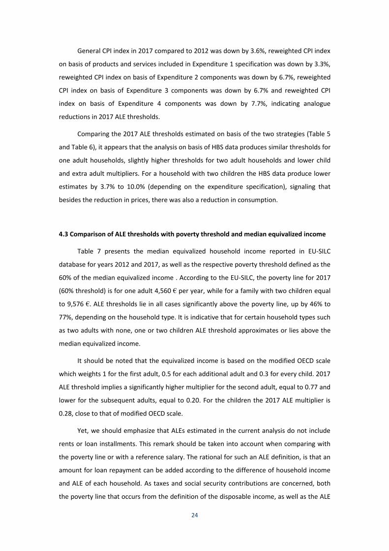
General CPI index in 2017 compared to 2012 was down by 3.6%, reweighted CPI index
on basis of products and services included in Expenditure 1 specification was down by 3.3%,
reweighted CPI index on basis of Expenditure 2 components was down by 6.7%, reweighted
CPI index on basis of Expenditure 3 components was down by 6.7% and reweighted CPI
index on basis of Expenditure 4 components was down by 7.7%, indicating analogue
reductions in 2017 ALE thresholds.
Comparing the 2017 ALE thresholds estimated on basis of the two strategies (Table 5
and Table 6), it appears that the analysis on basis of HBS data produces similar thresholds for
one adult households, slightly higher thresholds for two adult households and lower child
and extra adult multipliers. For a household with two children the HBS data produce lower
estimates by 3.7% to 10.0% (depending on the expenditure specification), signaling that
besides the reduction in prices, there was also a reduction in consumption.
4.3 Comparison of ALE thresholds with poverty threshold and median equivalized income
Table 7 presents the median equivalized household income reported in EU-SILC
database for years 2012 and 2017, as well as the respective poverty threshold defined as the
60% of the median equivalized income . According to the EU-SILC, the poverty line for 2017
(60% threshold) is for one adult 4,560 € per year, while for a family with two children equal
to 9,576 €. ALE thresholds lie in all cases significantly above the poverty line, up by 46% to
77%, depending on the household type. It is indicative that for certain household types such
as two adults with none, one or two children ALE threshold approximates or lies above the
median equivalized income.
It should be noted that the equivalized income is based on the modified OECD scale
which weights 1 for the first adult, 0.5 for each additional adult and 0.3 for every child. 2017
ALE threshold implies a significantly higher multiplier for the second adult, equal to 0.77 and
lower for the subsequent adults, equal to 0.20. For the children the 2017 ALE multiplier is
0.28, close to that of modified OECD scale.
Yet, we should emphasize that ALEs estimated in the current analysis do not include
rents or loan installments. This remark should be taken into account when comparing with
the poverty line or with a reference salary. The rational for such an ALE definition, is that an
amount for loan repayment can be added according to the difference of household income
and ALE of each household. As taxes and social security contributions are concerned, both
the poverty line that occurs from the definition of the disposable income, as well as the ALE

25
threshold are net of social security contributions and taxes. To this end, when designing
protection schemes, the eligibility of individuals should be judged on the basis of net
household income, removing all direct taxes (personal income tax, extra solidarity
contribution, property taxes), as well as social security contributions paid by household8.
Table 7: Comparison with poverty line and median equivalized income
Household type
Poverty
threshold (60%
of median
equivalised
income)
Median
equivalized
income (EU-
SILC)
ALE threshold
(Expenditure 3)
Ratio of ALE
with respect to
poverty
threshold
Ratio of ALE
with respect to
median
equivalized
income
2012 Single person 5,708 9,513 7,337 128.5% 77.1%
Two Adults 8,562 14,270 12,142 141.8% 85.1%
Child multiplier 1,712 2,854 2,955 172.6% 103.5%
Extra Adult multiplier 2,854 4,757 2,962 103.8% 62.3%
Two adults with one child 10,274 17,123 15,097 146.9% 88.2%
Two adults with one child and
one extra adult
13,128 21,880 18,059 137.6% 82.5%
Two adults with two children 11,986 19,977 18,052 150.6% 90.4%
Two adults with two children
and one extra adult
14,840 24,734 21,014 141.6% 85.0%
Two adults with three children 13,698 22,831 21,007 153.4% 92.0%
2017 Single person 4,560 7,600 6,853 150.3% 90.2%
Two Adults 6,840 11,400 12,121 177.2% 106.3%
Child multiplier 1,368 2,280 1,904 139.2% 83.5%
Extra Adult multiplier 2,280 3,800 1,376 60.4% 36.2%
Two adults with one child 8,208 13,680 14,025 170.9% 102.5%
Two adults with one child and
one extra adult
10,488 17,480 15,401 146.8% 88.1%
Two adults with two children 9,576 15,960 15,928 166.3% 99.8%
Two adults with two children
and one extra adult
11,856 19,760 17,304 146.0% 87.6%
Two adults with three children 10,944 18,240 17,832 162.9% 97.8%
Finally, with regards to the practical implementation of the ALEs Threshold, we should
emphasize that this must be considered as a lower limit, which should be revised upwards if
there are special circumstances in a household. Such examples are the presence of chronic ill
individuals, individuals with physical or mental health disabilities or with health problems
that need special pharmaceutical or surgical treatment, individuals paying marital
compensation and generally individuals having fixed annual expenses, which objectively
cannot be reduced.
8 See footnote 1.

26
4.4 Sensitivity analysis for the period 2010-2017
In order to evaluate the robustness of the methodology and the variation of the ALE
estimates through the years, we estimated the main specification A (with robust linear
regression) for the whole period 2010-2017, using the HBS data of each year acquired by
ELSTAT.
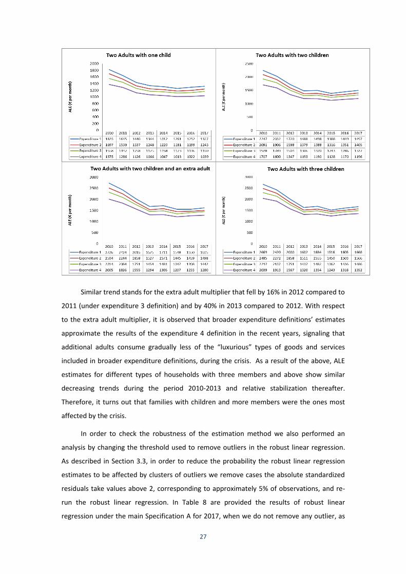
As observed in Figure 2, the ALE estimates for one adult and two adults households
fall in 2011 compared to 2010 (by 11.8% for one adult and by 8% for two adults, under
expenditure 3 definition), after the start of the implementation of the first economic
adjustment programme for Greece, and then remain at comparable levels thereafter with
both negative and positive fluctuations from one year to another. However, the child
multiplier continued to fall significantly both in years 2012 (by 29.3% compared to 2011
under expenditure 3) and 2013 (by 46.7% compared to 2012 under expenditure 3) and
remains at comparable low levels thereafter. This signals that given the budget constraints,
households with more members had to limit their total household expenditure throughout
the crisis, taking advantage of “economies of scale”, since many types of expenditures do
not rise linearly with the number of household members. It seems that during the period of
intense crisis, households gave priority to common expenses that offer utility to all members
of the household, rather than individual expenses that offer utility only to specific members.
Figure 2: Adequate Living expenses estimates for the period 2010-2017, based on specification A
(robust linear regression, mean) for different household types
27
Similar trend stands for the extra adult multiplier that fell by 16% in 2012 compared to
2011 (under expenditure 3 definition) and by 40% in 2013 compared to 2012. With respect
to the extra adult multiplier, it is observed that broader expenditure definitions’ estimates
approximate the results of the expenditure 4 definition in the recent years, signaling that
additional adults consume gradually less of the “luxurious” types of goods and services
included in broader expenditure definitions, during the crisis. As a result of the above, ALE
estimates for different types of households with three members and above show similar
decreasing trends during the period 2010-2013 and relative stabilization thereafter.
Therefore, it turns out that families with children and more members were the ones most
affected by the crisis.
In order to check the robustness of the estimation method we also performed an
analysis by changing the threshold used to remove outliers in the robust linear regression.
As described in Section 3.3, in order to reduce the probability the robust linear regression
estimates to be affected by clusters of outliers we remove cases the absolute standardized
residuals take values above 2, corresponding to approximately 5% of observations, and re-
run the robust linear regression. In Table 8 are provided the results of robust linear
regression under the main Specification A for 2017, when we do not remove any outlier, as

28
well as in the case we remove residuals with absolute value above 1.65. It is clear that the
removal of residuals with absolute value above 2 affects significantly the results of the
robust linear regression. These outliers as expected lie in the right tail of the distribution
(see also Figure 1) with mean yearly expenditure 37,996 €, as opposed to 13,947 € for the
rest of the sample. This signals that the robust linear regression is indeed significantly
affected by the top 5% of observations and thus the strategy followed to remove these, is in
the right direction to approximate the main mass of the distribution. However, removing
additional observations, i.e. for which the residuals take absolute values above 1.65, has a
rather smaller effect in the results whereas reducing further the sample size.
Table 8: Sensitivity analysis of robust linear regressions estimates on basis of percentage
of outliers removed
Yearly
Without
excluding outliers
Excluding residuals
with absolute value > 2
Excluding residuals with
absolute value > 1.65
One adult 7096 6853 6874
Two adults 13191 12121 11605
Child multiplier 2051 1904 2148
Extra Adult multiplier 1201 1376 1382
Two Adults with two children 17292 15928 15902
No. of observations removed 0 out of 14457
564 out of 14457,
corresponding to 4.8%
of the weighted sample
873 out of 14457,
corresponding to 8.0% of
the weighted sample
Mean outlier expenditure (std. dev.) 37996 (15257) 32605 (15687)
Mean sample expenditure (std. dev.) 15050 (9056) 13947 (6946) 13643 (6496)
Note: Are reported the 2017 Adequate Living expenses estimates on basis of Specification A and
Expenditure 3 definition.
Finally another sensitivity analysis conducted so as to approximate the ALE thresholds
of every year, was to run the robust liner regression estimation on basis of the total HBS
data of the whole 2010-2017 period and introduce dummies for each reference year and
interactions among years and the household synthesis variables. This strategy produced
results rather close to those reported above (i.e. with estimating every year separately), with
differences being less than 3% depending on the household type and reference year.
5. Conclusions
In this manuscript, we presented a general methodological framework to determine
the Adequate Living Expenses Threshold, based on the data from the Greek Household
Budget Survey in the period of crisis 2010-2017. We run numerous scenarios for alternative
expenditure compositions, adjusting for multiple effects, using different econometric

29
methods. The main scenarios proposed, lie in general much above the poverty line and
closer to the median income.
In view of the purpose of setting the ALE threshold for actual policy making decisions,
that counteract with other policies and need to endure a fairness across the income and
consumption distribution with regards to the protection of the first residence and the
allocation of possible state-subsidy to non-performing borrowers, we assume that the mean
or median family expenditure (after extracting non-prior and luxury expenses) should reflect
the adequate living expenses. This means that the approach is relative and in the case the
income and subsequently the expenditures of the sample population rise (fall), so does the
adequate living expenses threshold.
Although our article engages in a variety of computational estimations, the main
model proposed for policy use is the one explained by household composition. Besides the
fact that a policy tool must be practical and easy to be implemented, this is mainly done so
as to avoid social unfair situations in which poorer people have and lower ALE; rather we
seek to approximate an objective threshold applicable to the general population.
The alternative methodological approach (i.e. used in the case of Ireland and other
countries) would be to form task groups of experts, so as to synthesize baskets of goods and
services, a household is “reasonable” to consume, and evaluate their cost on a continuous
basis according to the CPI. Thus an estimation of the Adequate Living Expenses with this
method as well would be desirable, so as to identify any potential differences. Yet, the
basket method has the discrepancy that in period of rapid recession when all households are
losing income and are forced to squeeze their consumption, public policy design (like
protection and subsidy to non-performing borrowers) cannot depend on an “ideal” basket of
goods that not even the median household of the population can consume. Following such
an approach might lead to the design of regressive policies, which at the end harm the
poorest which never had access to borrowing or those that prioritize the repayment of their
debts towards satisfying other needs.
In total, the methodology proposed for the calculation of ALE possesses the advantage
of simplicity and transparency in calculations and ensures equity in the treatment across
different groups of the population and across the total income (consumption) distribution.
Therefore, its proper use in the design of public policies can generate a progressive effect in
terms of policy making. To this end, also the frequent update of the thresholds, if not every
year, but every two years is deemed necessary.

30
References
Aiyagari, S.R. (1994). “Uninsured idiosyncratic risk and aggregate saving.” The Quarterly
Journal of Economics, 109(3), 659-684.
Baker, S. (2018). “Debt and the Response to Household Income Shocks: Validation and
Application of Linked Financial Account Data.” Journal of Political Economics, 126(4),
1504-1557.
Ben-Gal I. (2005). “Outlier detection”, In: Maimon O. and Rockach L. (Eds.) Data Mining and
Knowledge Discovery Handbook: A Complete Guide for Practitioners and Researchers,
Kluwer Academic Publishers, ISBN 0-387-24435-2.
Brück, T., Danzer, A. M., Muravyev, A., & Weisshaar, N. (2010). “Poverty during transition:
Household survey evidence from Ukraine.” Journal of Comparative Economics, 38(2),
123-145.
Carroll, C., Dynan, K., & Krane, S. (2003). “Unemployment Risk and Precautionary Wealth:
Evidence from Households’ Balance Sheets.” Review of Economics and Statistics, 85(3),
586–604.
Citro, C. F. and R. T. Michael (1995). “Measuring poverty. A new approach.” Washington,
D.C., National Academy Press.
Collins, M.L., B. Mac Mahon, G. Weld and R. Thornton (2012). “A minimum income standard
for Ireland. A consensual budget standards study examining household types across the
lifecycle.” Studies in Public Policy No. 27, Dublin, Policy Institute, Trinity College Dublin.
Dynan, K., Mian, A., & Pence, K. M. (2012). “Is a household debt overhang holding back
consumption?” Brookings Papers on Economic Activity, Spring 2012, 299-362.
de Roiste, M., Fasianos, A., Kirkby, R., & Yao, F. (2019). “Household Leverage and
Asymmetric Housing Wealth Effects-Evidence from New Zealand.” Discussion Paper
Series No. DP2019/01, Reserve Bank of New Zealand.
European Consumer Debt Network (ECDN) (2009). “Reference Budgets for Social Inclusion.”
Money Matters no. 6.
Eurostat. EU-SILC database, available in: https://ec.europa.eu/eurostat/web/income-and-
living-conditions/data/database (accessed 02/2019).
Friedman, M. (1957). “A Theory of the Consumption Function.” National Bureau of Economic
Research. Princeton University Press, ISBN: 0-691-04182-2.
Goedemé, T., Storms, B., Stockman, S., Penne, T. and Van den Bosch, K., (2015). “Towards
cross-country comparable reference budgets in Europe: first results of a concerted
effort.” European Journal of Social Security, 17(1), 3-30.
Hellenic Statistical Authority (2018). “Household Budget Survey 2017.” Press Release,
Piraeus, 04/10/2018, Hellenic Statistical Authority.
Hoff, S., van Gaalen, C., Soede, A., Luten, A., Vrooman, C. and Lamers, S. (2010). “The
minimum agreed upon. Consensual budget standards for the Netherlands.” Den Hague,
The Netherlands Institute for Social Research, ISBN 978-90-377-0472-3.
31
Huber, P. (1964). “Robust Estimation of a Location Parameter.” Annals of Mathematical
Statistics, 35(1), 73-101.
Huber, P. (1981). “Robust Statistics.” New York: John Wiley and Sons.
IMF/EC/ECB (2013). “Guidance on Household Debt Definitions.” Report sent to the Greek
Government on 12/05/2013.
Insolvency Service of Ireland (ISI) (2013). “Guidelines on a reasonable standard of living and
reasonable living expenses.” Dublin.
Kemmetmüller, M. and Leitner, K. (2009). “The development of Reference Budgets in
Austria.” 3rd ecdn General Assembly and Conference Reference Budgets for Social
Inclusion, Vienna.
Koenker, R. (2005). “Quantile Regression.” Cambridge University Press. ISBN 0-521-60827-9.
Konsument Verket (2009). “Estimated costs of living. The basis of decision making for
reference budgets and budget advising in Sweden.” Karlstad: The Swedish Consumer
Agency, Report 2009:8.
Modigliani, F. and R. Brumberg (1954). “Utility Analysis and the Consumption Function: An
Interpretation of Cross-Section Data.” Post Keynesian Economics, 6, 388-436.
Muller, C. (2002). “Prices and living standards: evidence for Rwanda.” Journal of
Development Economics, 68(1), 187-203.
Muller, C. and Bibi, S. (2010). “Refining targeting against poverty evidence from Tunisia.”
Oxford Bulletin of Economics and Statistics, 72(3), 381-410.
Penne, T., Cornelis, I. and Storms, B., (2019). “Reducing out-of-pocket costs to improve the
adequacy of minimum income protection? Reference budgets as an EU policy indicator:
the Belgian case.” Herman Deleeck Centre for Spocial Policy, Working paper No. 19.06,
University of Antwerp.
Preuße, H. (2012). "Reference budgets for counselling on how to manage private household
finance–requirements and patterns based on international experience." International
Journal of Consumer Studies, 36(5), 602-610.
Rousseeuw, P. J. and A.M. Leroy. (1987). “Robust Regression and Outlier Detection.” New
York: Wiley.
Rousseeuw, P. J. and B. Van Zomeren. (1990). “Unmasking Multivariate Outliers and
Leverage Points.” Journal of the American Statistical Association, 85, 633-639.
Storms, B., Goedemé, T., Van den Bosch, K., Penne, T., Schuerman, N., Stockman, S. (2014).
“Pilot project for the development of a common methodology on reference budgets in
Europe: Review of current state of play on reference budget practices at national,
regional, and local level.” Employment, Social Affairs & Inclusion, European Commission.
32
ANNEX A:
Alternative adequate living expenses estimates based on
various model specifications

33
Table A.1: Adequate Living Expenses estimates (in €) based on Expenditure 1 and various
model specifications, for the years 2012 and 2017
Specification A Specification B Specification C
2017 ALE thresholds 2017 ALE thresholds 2017 ALE thresholds
All households Non Mortgage
holders Mortgage holders
Urban or semi-
urban region
Agricultural
region
Yearly Mean Median Yearly Mean Median Mean Median Yearly Mean Median Mean Median
One adult 7771 6688 One adult 7684 6625 10468 8767 One adult 7945 6855 7137 6051
Two adults 13877 12354 Two adults 13540 11994 16343 15701 Two adults 14142 12803 12693 10786
Child
multiplier 2046 2447
Child
multiplier 1983 2373 1910 2237
Child
multiplier 2013 2396 2175 3013
Extra Adult
multiplier 1415 2170
Extra Adult
multiplier 1787 2469 144 1001
Extra Adult
multiplier 2006 2450 1333 1859
Two Adults
with two
children
17968 17248
Two Adults
with two
children
17505 16741 20163 20175
Two Adults
with two
children
18167 17596 17043 16812
Monthly Mean Median Monthly Mean Median Mean Median Monthly Mean Median Mean Median
One adult 648 557 One adult 640 552 872 731 One adult 662 571 595 504
Two adults 1156 1029 Two adults 1128 1000 1362 1308 Two adults 1178 1067 1058 899
Child
multiplier 170 204
Child
multiplier 165 198 159 186
Child
multiplier 168 200 181 251
Extra Adult
multiplier 118 181
Extra Adult
multiplier 149 206 12 83
Extra Adult
multiplier 167 204 111 155
Two Adults
with two
children
1497 1437
Two Adults
with two
children
1459 1395 1680 1681
Two Adults
with two
children
1514 1466 1420 1401
2012 ALE thresholds 2012 ALE thresholds 2012 ALE thresholds
All households Non Mortgage
holders Mortgage holders
Urban or semi-
urban region
Agricultural
region
Yearly Mean Median Yearly Mean Median Mean Median Yearly Mean Median Mean Median
One adult 8180 6392 One adult 7894 6196 13278 11025 One adult 8499 6932 7444 5813
Two adults 13917 11833 Two adults 13438 11448 18530 16571 Two adults 14275 13042 13447 11445
Child
multiplier 3361 4157
Child
multiplier 3104 3971 2367 2171
Child
multiplier 3483 4336 3172 3866
Extra Adult
multiplier 3550 3880
Extra Adult
multiplier 3614 4005 2225 3120
Extra Adult
multiplier 4168 4347 2815 3531
Two Adults
with two
children
20639 20147
Two Adults
with two
children
19645 19389 23265 20914
Two Adults
with two
children
21241 21713 19791 19176
Monthly Mean Median Monthly Mean Median Mean Median Monthly Mean Median Mean Median
One adult 682 533 One adult 658 516 1107 919 One adult 708 578 620 484
Two adults 1160 986 Two adults 1120 954 1544 1381 Two adults 1190 1087 1121 954
Child
multiplier 280 346
Child
multiplier 259 331 197 181
Child
multiplier 290 361 264 322
Extra Adult
multiplier 296 323
Extra Adult
multiplier 301 334 185 260
Extra Adult
multiplier 347 362 235 294
Two Adults
with two
children
1720 1679
Two Adults
with two
children
1637 1616 1939 1743
Two Adults
with two
children
1770 1809 1649 1598
Notes: Specifications A, B and C are denoted in Section 3.3 and Expenditure 1 synthesis in Table 1. Mean
estimates are based on robust linear regression and median estimates on basis of quantile regression.

34
Table A.2: Adequate Living Expenses estimates (in €) based on Expenditure 2 and various
model specifications, for the years 2012 and 2017
Specification A Specification B Specification C
2017 ALE thresholds 2017 ALE thresholds 2017 ALE thresholds
All households Non Mortgage
holders Mortgage holders
Urban or semi-
urban region
Agricultural
region
Yearly Mean Median Yearly Mean Median Mean Median Yearly Mean Median Mean Median
One adult 7180 6256 One adult 7100 6227 9888 8241 One adult 7327 6440 6661 5723
Two adults 13285 11922 Two adults 12699 11150 15263 14635 Two adults 13277 11884 11791 10178
Child
multiplier 1942 2515
Child
multiplier 1892 2384 1820 2081
Child
multiplier 1890 2269 1224 1552
Extra Adult
multiplier 1121 1842
Extra Adult
multiplier 1408 2029 183 839
Extra Adult
multiplier 1529 2093 1158 1606
Two Adults
with two
children
17168 16952
Two Adults
with two
children
16484 15918 18902 18798
Two Adults
with two
children
17058 16422 14240 13282
Monthly Mean Median Monthly Mean Median Mean Median Monthly Mean Median Mean Median
One adult 598 521 One adult 592 519 824 687 One adult 611 537 555 477
Two adults 1107 993 Two adults 1058 929 1272 1220 Two adults 1106 990 983 848
Child
multiplier 162 210
Child
multiplier 158 199 152 173
Child
multiplier 158 189 102 129
Extra Adult
multiplier 93 154
Extra Adult
multiplier 117 169 15 70
Extra Adult
multiplier 127 174 97 134
Two Adults
with two
children
1431 1413
Two Adults
with two
children
1374 1327 1575 1566
Two Adults
with two
children
1421 1369 1187 1107
2012 ALE thresholds 2012 ALE thresholds 2012 ALE thresholds
All households Non Mortgage
holders Mortgage holders
Urban or semi-
urban region
Agricultural
region
Yearly Mean Median Yearly Mean Median Mean Median Yearly Mean Median Mean Median
One adult 7655 6082 One adult 7362 5896 12463 10841 One adult 7819 6416 7123 5314
Two adults 12921 11076 Two adults 12482 10836 17255 15679 Two adults 13247 11397 12514 10640
Child
multiplier 3126 3884
Child
multiplier 2998 3475 2385 2105
Child
multiplier 3372 5871 2955 3340
Extra Adult
multiplier 3117 3551
Extra Adult
multiplier 3000 3458 1891 2446
Extra Adult
multiplier 3651 3585 2338 2864
Two Adults
with two
children
19173 18845
Two Adults
with two
children
18478 17785 22025 19889
Two Adults
with two
children
19991 23138 18424 17319
Monthly Mean Median Monthly Mean Median Mean Median Monthly Mean Median Mean Median
One adult 638 507 One adult 613 491 1039 903 One adult 652 535 594 443
Two adults 1077 923 Two adults 1040 903 1438 1307 Two adults 1104 950 1043 887
Child
multiplier 261 324
Child
multiplier 250 290 199 175
Child
multiplier 281 489 246 278
Extra Adult
multiplier 260 296
Extra Adult
multiplier 250 288 158 204
Extra Adult
multiplier 304 299 195 239
Two Adults
with two
children
1598 1570
Two Adults
with two
children
1540 1482 1835 1657
Two Adults
with two
children
1666 1928 1535 1443
Notes: Specifications A, B and C are denoted in Section 3.3 and Expenditure 2 synthesis in Table 1. Mean
estimates are based on robust linear regression and median estimates on basis of quantile regression.

35
Table A.3: Adequate Living Expenses estimates (in €) based on Expenditure 3 and various
model specifications, for the years 2012 and 2017
Specification A Specification B Specification C
2017 ALE thresholds 2017 ALE thresholds 2017 ALE thresholds
All households Non Mortgage
holders Mortgage holders
Urban or semi-
urban region
Agricultural
region
Yearly Mean Median Yearly Mean Median Mean Median Yearly Mean Median Mean Median
One adult 6853 6112 One adult 6826 6086 9299 8121 One adult 7013 6295 6327 5555
Two adults 12121 10981 Two adults 11897 10784 14417 13235 Two adults 12446 11344 11155 9876
Child
multiplier 1904 2388
Child
multiplier 1688 2246 2137 2315
Child
multiplier 1744 2187 2472 2891
Extra Adult
multiplier 1376 1917
Extra Adult
multiplier 1591 2114 233 1475
Extra Adult
multiplier 1665 2137 915 1553
Two Adults
with two
children
15928 15756
Two Adults
with two
children
15274 15276 18691 17864
Two Adults
with two
children
15934 15718 16098 15657
Monthly Mean Median Monthly Mean Median Mean Median Monthly Mean Median Mean Median
One adult 571 509 One adult 569 507 775 677 One adult 584 525 527 463
Two adults 1010 915 Two adults 991 899 1201 1103 Two adults 1037 945 930 823
Child
multiplier 159 199
Child
multiplier 141 187 178 193
Child
multiplier 145 182 206 241
Extra Adult
multiplier 115 160
Extra Adult
multiplier 133 176 19 123
Extra Adult
multiplier 139 178 76 129
Two Adults
with two
children
1327 1313
Two Adults
with two
children
1273 1273 1558 1489
Two Adults
with two
children
1328 1310 1342 1305
2012 ALE thresholds 2012 ALE thresholds 2012 ALE thresholds
All households Non Mortgage
holders Mortgage holders
Urban or semi-
urban region
Agricultural
region
Yearly Mean Median Yearly Mean Median Mean Median Yearly Mean Median Mean Median
One adult 7337 5896 One adult 7166 5794 12055 11501 One adult 7636 6124 7046 5245
Two adults 12142 10906 Two adults 11859 10549 16219 15485 Two adults 12356 11271 11831 10353
Child
multiplier 2955 3440
Child
multiplier 2765 3358 2057 1696
Child
multiplier 3147 4041 2685 3211
Extra Adult
multiplier 2962 3294
Extra Adult
multiplier 2828 3251 1909 2543
Extra Adult
multiplier 3499 3983 2275 2556
Two Adults
with two
children
18052 17785
Two Adults
with two
children
17389 17266 20333 18878
Two Adults
with two
children
18650 19353 17200 16774
Monthly Mean Median Monthly Mean Median Mean Median Monthly Mean Median Mean Median
One adult 611 491 One adult 597 483 1005 958 One adult 636 510 587 437
Two adults 1012 909 Two adults 988 879 1352 1290 Two adults 1030 939 986 863
Child
multiplier 246 287
Child
multiplier 230 280 171 141
Child
multiplier 262 337 224 268
Extra Adult
multiplier 247 275
Extra Adult
multiplier 236 271 159 212
Extra Adult
multiplier 292 332 190 213
Two Adults
with two
children
1504 1482
Two Adults
with two
children
1449 1439 1694 1573
Two Adults
with two
children
1554 1613 1433 1398
Notes: Specifications A, B and C are denoted in Section 3.3 and Expenditure 3 synthesis in Table 1. Mean
estimates are based on robust linear regression and median estimates on basis of quantile regression.
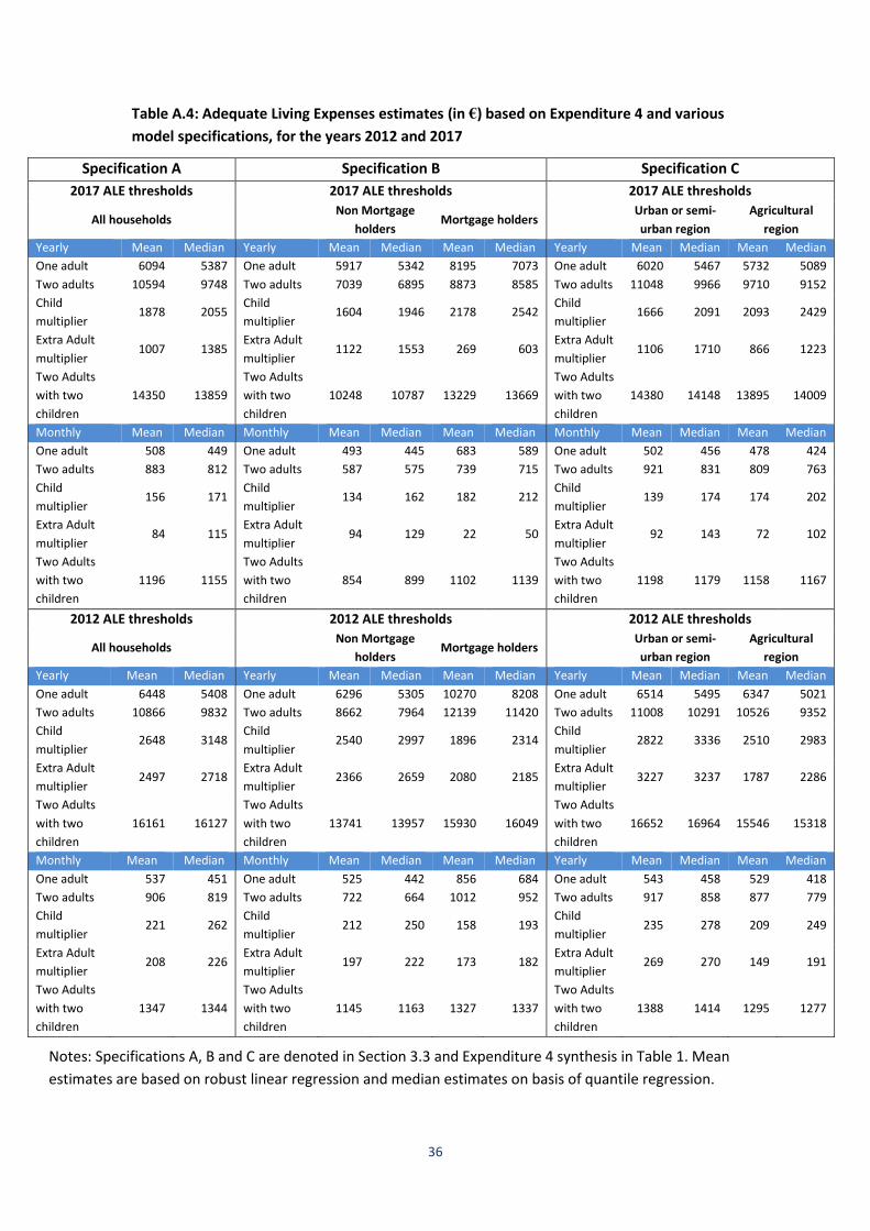
36
Table A.4: Adequate Living Expenses estimates (in €) based on Expenditure 4 and various
model specifications, for the years 2012 and 2017
Specification A Specification B Specification C
2017 ALE thresholds 2017 ALE thresholds 2017 ALE thresholds
All households Non Mortgage
holders Mortgage holders
Urban or semi-
urban region
Agricultural
region
Yearly Mean Median Yearly Mean Median Mean Median Yearly Mean Median Mean Median
One adult 6094 5387 One adult 5917 5342 8195 7073 One adult 6020 5467 5732 5089
Two adults 10594 9748 Two adults 7039 6895 8873 8585 Two adults 11048 9966 9710 9152
Child
multiplier 1878 2055
Child
multiplier 1604 1946 2178 2542
Child
multiplier 1666 2091 2093 2429
Extra Adult
multiplier 1007 1385
Extra Adult
multiplier 1122 1553 269 603
Extra Adult
multiplier 1106 1710 866 1223
Two Adults
with two
children
14350 13859
Two Adults
with two
children
10248 10787 13229 13669
Two Adults
with two
children
14380 14148 13895 14009
Monthly Mean Median Monthly Mean Median Mean Median Monthly Mean Median Mean Median
One adult 508 449 One adult 493 445 683 589 One adult 502 456 478 424
Two adults 883 812 Two adults 587 575 739 715 Two adults 921 831 809 763
Child
multiplier 156 171
Child
multiplier 134 162 182 212
Child
multiplier 139 174 174 202
Extra Adult
multiplier 84 115
Extra Adult
multiplier 94 129 22 50
Extra Adult
multiplier 92 143 72 102
Two Adults
with two
children
1196 1155
Two Adults
with two
children
854 899 1102 1139
Two Adults
with two
children
1198 1179 1158 1167
2012 ALE thresholds 2012 ALE thresholds 2012 ALE thresholds
All households Non Mortgage
holders Mortgage holders
Urban or semi-
urban region
Agricultural
region
Yearly Mean Median Yearly Mean Median Mean Median Yearly Mean Median Mean Median
One adult 6448 5408 One adult 6296 5305 10270 8208 One adult 6514 5495 6347 5021
Two adults 10866 9832 Two adults 8662 7964 12139 11420 Two adults 11008 10291 10526 9352
Child
multiplier 2648 3148
Child
multiplier 2540 2997 1896 2314
Child
multiplier 2822 3336 2510 2983
Extra Adult
multiplier 2497 2718
Extra Adult
multiplier 2366 2659 2080 2185
Extra Adult
multiplier 3227 3237 1787 2286
Two Adults
with two
children
16161 16127
Two Adults
with two
children
13741 13957 15930 16049
Two Adults
with two
children
16652 16964 15546 15318
Monthly Mean Median Monthly Mean Median Mean Median Yearly Mean Median Mean Median
One adult 537 451 One adult 525 442 856 684 One adult 543 458 529 418
Two adults 906 819 Two adults 722 664 1012 952 Two adults 917 858 877 779
Child
multiplier 221 262
Child
multiplier 212 250 158 193
Child
multiplier 235 278 209 249
Extra Adult
multiplier 208 226
Extra Adult
multiplier 197 222 173 182
Extra Adult
multiplier 269 270 149 191
Two Adults
with two
children
1347 1344
Two Adults
with two
children
1145 1163 1327 1337
Two Adults
with two
children
1388 1414 1295 1277
Notes: Specifications A, B and C are denoted in Section 3.3 and Expenditure 4 synthesis in Table 1. Mean
estimates are based on robust linear regression and median estimates on basis of quantile regression.

37
ANNEX B:
Regression results

38
Table B.1: Regression results based on Expenditure 1 and various model specifications, for
the years 2012 and 2017
2012 ALE estimates 2017 ALE estimates
Specification A
Robust linear regression
(mean)
Quantile reggression
(median)
Robust linear regression
(mean)
Quantile reggression
(median)
Variable Coef.
Std.
Err. P>|t| Coef.
Std.
Err. P>|t| Coef.
Std.
Err. P>|t| Coef.
Std.
Err. P>|t|
num_dep_children 3361.00 3.39 0.00 4157.04 6.78 0.00 2045.56 2.11 0.00 2447.28 2.39 0.00
dummy_twoplus_adu
lts
5736.89 7.61 0.00 5441.16 21.01 0.00 6105.32 6.09 0.00 5665.92 9.10 0.00
num_add_adults 3550.47 4.80 0.00 3879.72 9.16 0.00 1415.38 3.08 0.00 2169.90 3.17 0.00
_cons 8179.93 6.32 0.00 6391.80 19.09 0.00 7771.37 4.71 0.00 6687.96 8.15 0.00
R-squared = 0.175 Pseudo R-squared = 0.095 R-squared = 0.202 Pseudo R-squared =0.126
Specification B
Robust linear regression
(mean)
Quantile reggression
(median)
Robust linear regression
(mean)
Quantile reggression
(median)
Variable Coef.
Std.
Err. P>|t| Coef.
Std.
Err. P>|t| Coef.
Std.
Err. P>|t| Coef.
Std.
Err. P>|t|
num_dep_children 3103.77 3.49 0.00 3970.56 3.89 0.00 1982.99 2.46 0.00 2373.24 2.94 0.00
dummy_twoplus_adu
lts
5543.20 7.56 0.00 5252.52 11.57 0.00 5855.67 6.23 0.00 5369.40 10.24 0.00
num_add_adults 3613.96 5.06 0.00 4004.88 5.32 0.00 1787.39 3.70 0.00 2468.64 3.83 0.00
dummy_mortgage 5383.86 30.31 0.00 4828.92 42.18 0.00 2784.17 31.88 0.00 2142.24 46.57 0.00
int_twoplus_adults_
mortgage
-291.26 30.89 0.00 294.00 43.11 0.00 19.12 33.92 0.57 1564.73 48.28 0.00
int_num_dep_childre
n_mortgage
-736.48 10.90 0.00 -1799.16 10.55 0.00 -72.74 4.71 0.00 -136.37 6.73 0.00
int_num_add_adults_
mortgage
-1388.53 15.10 0.00 -884.40 12.98 0.00 -1643.06 6.30 0.00 -1467.62 9.08 0.00
_cons 7894.38 6.13 0.00 6195.84 10.41 0.00 7683.84 4.70 0.00 6625.08 9.09 0.00
R-squared = 0.192 Pseudo R-squared = 0.101 R-squared =0.213 Pseudo R-squared =0.131
Specification C
Robust linear regression
(mean)
Quantile reggression
(median)
Robust linear regression
(mean)
Quantile reggression
(median)
Variable Coef.
Std.
Err. P>|t| Coef.
Std.
Err. P>|t| Coef.
Std.
Err. P>|t| Coef.
Std.
Err. P>|t|
num_dep_children 3482.82 4.60 0.00 4335.72 2.E-12 0.00 2012.61 2.51 0.00 2396.35 2.46 0.00
dummy_twoplus_adu
lts
5776.23 9.67 0.00 6109.32 6.E-12 0.00 6196.38 7.24 0.00 5947.68 9.03 0.00
num_add_adults 4167.86 6.35 0.00 4347.12 3.E-12 0.00 2006.28 3.80 0.00 2450.28 3.75 0.00
dummy_agr -1054.53 12.78 0.00 -1119.24 9.E-12 0.00 -807.74 9.96 0.00 -803.76 17.59 0.00
int_twoplus_adults_a
gr
226.24 15.34 0.00 -476.88 1.E-11 0.00 -641.29 12.55 0.00 -1212.96 19.44 0.00
int_num_dep_childre
n_agr
-310.74 6.60 0.00 -470.22 3.E-12 0.00 162.79 4.69 0.00 616.65 4.69 0.00
int_num_add_adults_
agr
-1352.49 9.52 0.00 -816.24 4.E-12 0.00 -673.06 6.31 0.00 -591.00 5.69 0.00
_cons 8498.90 7.78 0.00 6932.28 6.E-12 0.00 7945.17 5.50 0.00 6855.24 8.04 0.00
R-squared = 0.181 Pseudo R-squared = 0.101 R-squared =0.212 Pseudo R-squared = 0.131
Notes: Specifications A, B and C are denoted in Section 3.3 and Expenditure 1 synthesis in Table 1.

39
Table B.2: Regression results based on Expenditure 2 and various model specifications, for
the years 2012 and 2017
2012 ALE estimates 2017 ALE estimates
Specification A
Robust linear regression
(mean)
Quantile reggression (median) Robust linear regression
(mean)
Quantile reggression
(median)
Variable Coef.
Std.
Err. P>|t| Coef.
Std.
Err. P>|t| Coef.
Std.
Err. P>|t| Coef.
Std.
Err. P>|t|
num_dep_children 3126.38 3.08 0.00 3884.38 0.66 0.00 1941.65 1.99 0.00 2515.04 1.51 0.00
dummy_twoplus_a
dults
5265.99 7.01 0.00 4993.58 2.04 0.00 5792.00 5.47 0.00 5116.72 5.76 0.00
num_add_adults 3117.32 4.33 0.00 3550.88 0.89 0.00 1120.74 2.88 0.00 1842.28 2.01 0.00
_cons 7654.61 5.82 0.00 6082.34 1.86 0.00 7179.60 4.19 0.00 6255.60 5.16 0.00
R-squared = 0.175 Pseudo R-squared = 0.096 R-squared = 0.205 Pseudo R-squared =0.120
Specification B
Robust linear regression
(mean)
Quantile reggression (median) Robust linear regression
(mean)
Quantile reggression
(median)
Variable Coef.
Std.
Err. P>|t| Coef.
Std.
Err. P>|t| Coef.
Std.
Err. P>|t| Coef.
Std.
Err. P>|t|
num_dep_children 2998.29 3.24 0.00 3474.54 4.06 0.00 1892.42 2.33 0.00 2383.98 2.13 0.00
dummy_twoplus_a
dults
5120.27 7.01 0.00 4940.16 12.07 0.00 5598.23 5.61 0.00 4923.36 7.43 0.00
num_add_adults 2999.74 4.45 0.00 3458.34 5.55 0.00 1408.25 3.47 0.00 2029.08 2.78 0.00
dummy_mortgage 5101.12 28.10 0.00 4945.32 44.00 0.00 2787.59 30.32 0.00 2013.84 33.79 0.00
int_twoplus_adults
_mortgage
-328.13 28.66 0.00 -102.12 44.98 0.02 -223.71 32.06 0.00 1471.44 35.03 0.00
int_num_dep_child
ren_mortgage
-613.30 10.13 0.00 -1369.62 11.00 0.00 -72.76 4.50 0.00 -302.94 4.89 0.00
int_num_add_adult
s_mortgage
-1108.59 14.10 0.00 -1012.50 13.54 0.00 -1225.42 6.04 0.00 -1189.80 6.59 0.00
_cons 7361.59 5.70 0.00 5895.60 10.86 0.00 7100.43 4.18 0.00 6226.80 6.60 0.00
R-squared = 0.193 Pseudo R-squared = 0.102 R-squared = 0.214 Pseudo R-squared = 0.128
Specification C
Robust linear regression
(mean)
Quantile reggression (median) Robust linear regression
(mean)
Quantile reggression
(median)
Variable Coef.
Std.
Err. P>|t| Coef. Std. Err. P>|t| Coef.
Std.
Err. P>|t| Coef.
Std.
Err. P>|t|
num_dep_children 3371.99 4.32 0.00 5870.58 132.45 0.00 1890.34 2.33 0.00 2269.02 3.12 0.00
dummy_twoplus_a
dults
5428.16 8.88 0.00 4981.08 384.77 0.00 5949.93 6.50 0.00 5444.15 11.45 0.00
num_add_adults 3650.55 5.84 0.00 3584.88 181.50 0.00 1529.16 3.47 0.00 2093.28 4.76 0.00
dummy_agr -696.48 11.99 0.00 -1101.96 570.60 0.05 -666.22 8.83 0.00 -716.76 22.31 0.00
int_twoplus_adults
_agr
-37.02 14.33 0.01 344.88 625.14 0.58 -819.57 11.29 0.00 -989.51 24.66 0.00
int_num_dep_child
ren_agr
-416.67 6.12 0.00 -2530.86 196.09 0.00 220.50 4.51 0.00 656.82 5.95 0.00
int_num_add_adult
s_agr
-1312.20 8.52 0.00 -720.48 263.71 0.01 -371.16 5.94 0.00 -487.02 7.22 0.00
_cons 7819.10 7.04 0.00 6415.80 345.77 0.00 7327.29 4.89 0.00 6440.04 10.20 0.00
R-squared = 0.183 Pseudo R-squared = 0.102 R-squared =0.213 Pseudo R-squared = 0.127
Notes: Specifications A, B and C are denoted in Section 3.3 and Expenditure 2 synthesis in Table 1.
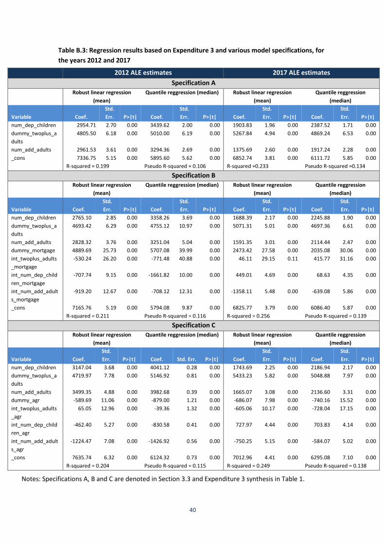
40
Table B.3: Regression results based on Expenditure 3 and various model specifications, for
the years 2012 and 2017
2012 ALE estimates 2017 ALE estimates
Specification A
Robust linear regression
(mean)
Quantile reggression (median) Robust linear regression
(mean)
Quantile reggression
(median)
Variable Coef.
Std.
Err. P>|t| Coef.
Std.
Err. P>|t| Coef.
Std.
Err. P>|t| Coef.
Std.
Err. P>|t|
num_dep_children 2954.71 2.70 0.00 3439.62 2.00 0.00 1903.83 1.96 0.00 2387.52 1.71 0.00
dummy_twoplus_a
dults
4805.50 6.18 0.00 5010.00 6.19 0.00 5267.84 4.94 0.00 4869.24 6.53 0.00
num_add_adults 2961.53 3.61 0.00 3294.36 2.69 0.00 1375.69 2.60 0.00 1917.24 2.28 0.00
_cons 7336.75 5.15 0.00 5895.60 5.62 0.00 6852.74 3.81 0.00 6111.72 5.85 0.00
R-squared = 0.199 Pseudo R-squared = 0.106 R-squared =0.233 Pseudo R-squared =0.134
Specification B
Robust linear regression
(mean)
Quantile reggression (median) Robust linear regression
(mean)
Quantile reggression
(median)
Variable Coef.
Std.
Err. P>|t| Coef.
Std.
Err. P>|t| Coef.
Std.
Err. P>|t| Coef.
Std.
Err. P>|t|
num_dep_children 2765.10 2.85 0.00 3358.26 3.69 0.00 1688.39 2.17 0.00 2245.88 1.90 0.00
dummy_twoplus_a
dults
4693.42 6.29 0.00 4755.12 10.97 0.00 5071.31 5.01 0.00 4697.36 6.61 0.00
num_add_adults 2828.32 3.76 0.00 3251.04 5.04 0.00 1591.35 3.01 0.00 2114.44 2.47 0.00
dummy_mortgage 4889.69 25.73 0.00 5707.08 39.99 0.00 2473.42 27.58 0.00 2035.08 30.06 0.00
int_twoplus_adults
_mortgage
-530.24 26.20 0.00 -771.48 40.88 0.00 46.11 29.15 0.11 415.77 31.16 0.00
int_num_dep_child
ren_mortgage
-707.74 9.15 0.00 -1661.82 10.00 0.00 449.01 4.69 0.00 68.63 4.35 0.00
int_num_add_adult
s_mortgage
-919.20 12.67 0.00 -708.12 12.31 0.00 -1358.11 5.48 0.00 -639.08 5.86 0.00
_cons 7165.76 5.19 0.00 5794.08 9.87 0.00 6825.77 3.79 0.00 6086.40 5.87 0.00
R-squared = 0.211 Pseudo R-squared = 0.116 R-squared = 0.256 Pseudo R-squared = 0.139
Specification C
Robust linear regression
(mean)
Quantile reggression (median) Robust linear regression
(mean)
Quantile reggression
(median)
Variable Coef.
Std.
Err. P>|t| Coef. Std. Err. P>|t| Coef.
Std.
Err. P>|t| Coef.
Std.
Err. P>|t|
num_dep_children 3147.04 3.68 0.00 4041.12 0.28 0.00 1743.69 2.25 0.00 2186.94 2.17 0.00
dummy_twoplus_a
dults
4719.97 7.78 0.00 5146.92 0.81 0.00 5433.23 5.82 0.00 5048.88 7.97 0.00
num_add_adults 3499.35 4.88 0.00 3982.68 0.39 0.00 1665.07 3.08 0.00 2136.60 3.31 0.00
dummy_agr -589.69 11.06 0.00 -879.00 1.21 0.00 -686.07 7.98 0.00 -740.16 15.52 0.00
int_twoplus_adults
_agr
65.05 12.96 0.00 -39.36 1.32 0.00 -605.06 10.17 0.00 -728.04 17.15 0.00
int_num_dep_child
ren_agr
-462.40 5.27 0.00 -830.58 0.41 0.00 727.97 4.44 0.00 703.83 4.14 0.00
int_num_add_adult
s_agr
-1224.47 7.08 0.00 -1426.92 0.56 0.00 -750.25 5.15 0.00 -584.07 5.02 0.00
_cons 7635.74 6.32 0.00 6124.32 0.73 0.00 7012.96 4.41 0.00 6295.08 7.10 0.00
R-squared = 0.204 Pseudo R-squared = 0.115 R-squared = 0.249 Pseudo R-squared = 0.138
Notes: Specifications A, B and C are denoted in Section 3.3 and Expenditure 3 synthesis in Table 1.
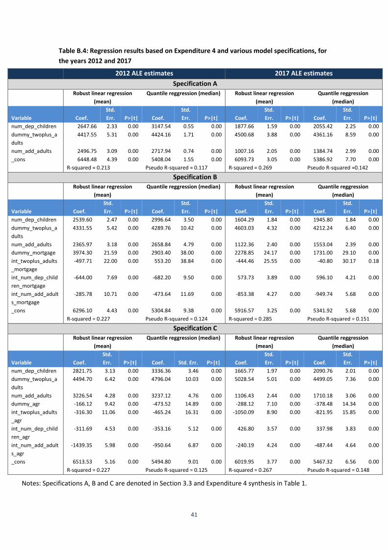
41
Table B.4: Regression results based on Expenditure 4 and various model specifications, for
the years 2012 and 2017
2012 ALE estimates 2017 ALE estimates
Specification A
Robust linear regression
(mean)
Quantile reggression (median) Robust linear regression
(mean)
Quantile reggression
(median)
Variable Coef.
Std.
Err. P>|t| Coef.
Std.
Err. P>|t| Coef.
Std.
Err. P>|t| Coef.
Std.
Err. P>|t|
num_dep_children 2647.66 2.33 0.00 3147.54 0.55 0.00 1877.66 1.59 0.00 2055.42 2.25 0.00
dummy_twoplus_a
dults
4417.55 5.31 0.00 4424.16 1.71 0.00 4500.68 3.88 0.00 4361.16 8.59 0.00
num_add_adults 2496.75 3.09 0.00 2717.94 0.74 0.00 1007.16 2.05 0.00 1384.74 2.99 0.00
_cons 6448.48 4.39 0.00 5408.04 1.55 0.00 6093.73 3.05 0.00 5386.92 7.70 0.00
R-squared = 0.213 Pseudo R-squared = 0.117 R-squared = 0.269 Pseudo R-squared =0.142
Specification B
Robust linear regression
(mean)
Quantile reggression (median) Robust linear regression
(mean)
Quantile reggression
(median)
Variable Coef.
Std.
Err. P>|t| Coef.
Std.
Err. P>|t| Coef.
Std.
Err. P>|t| Coef.
Std.
Err. P>|t|
num_dep_children 2539.60 2.47 0.00 2996.64 3.50 0.00 1604.29 1.84 0.00 1945.80 1.84 0.00
dummy_twoplus_a
dults
4331.55 5.42 0.00 4289.76 10.42 0.00 4603.03 4.32 0.00 4212.24 6.40 0.00
num_add_adults 2365.97 3.18 0.00 2658.84 4.79 0.00 1122.36 2.40 0.00 1553.04 2.39 0.00
dummy_mortgage 3974.30 21.59 0.00 2903.40 38.00 0.00 2278.85 24.17 0.00 1731.00 29.10 0.00
int_twoplus_adults
_mortgage
-497.71 22.00 0.00 553.20 38.84 0.00 -444.46 25.55 0.00 -40.80 30.17 0.18
int_num_dep_child
ren_mortgage
-644.00 7.69 0.00 -682.20 9.50 0.00 573.73 3.89 0.00 596.10 4.21 0.00
int_num_add_adult
s_mortgage
-285.78 10.71 0.00 -473.64 11.69 0.00 -853.38 4.27 0.00 -949.74 5.68 0.00
_cons 6296.10 4.43 0.00 5304.84 9.38 0.00 5916.57 3.25 0.00 5341.92 5.68 0.00
R-squared = 0.227 Pseudo R-squared = 0.124 R-squared = 0.285 Pseudo R-squared = 0.151
Specification C
Robust linear regression
(mean)
Quantile reggression (median) Robust linear regression
(mean)
Quantile reggression
(median)
Variable Coef.
Std.
Err. P>|t| Coef. Std. Err. P>|t| Coef.
Std.
Err. P>|t| Coef.
Std.
Err. P>|t|
num_dep_children 2821.75 3.13 0.00 3336.36 3.46 0.00 1665.77 1.97 0.00 2090.76 2.01 0.00
dummy_twoplus_a
dults
4494.70 6.42 0.00 4796.04 10.03 0.00 5028.54 5.01 0.00 4499.05 7.36 0.00
num_add_adults 3226.54 4.28 0.00 3237.12 4.76 0.00 1106.43 2.44 0.00 1710.18 3.06 0.00
dummy_agr -166.12 9.42 0.00 -473.52 14.89 0.00 -288.12 7.10 0.00 -378.48 14.34 0.00
int_twoplus_adults
_agr
-316.30 11.06 0.00 -465.24 16.31 0.00 -1050.09 8.90 0.00 -821.95 15.85 0.00
int_num_dep_child
ren_agr
-311.69 4.53 0.00 -353.16 5.12 0.00 426.80 3.57 0.00 337.98 3.83 0.00
int_num_add_adult
s_agr
-1439.35 5.98 0.00 -950.64 6.87 0.00 -240.19 4.24 0.00 -487.44 4.64 0.00
_cons 6513.53 5.16 0.00 5494.80 9.01 0.00 6019.95 3.77 0.00 5467.32 6.56 0.00
R-squared = 0.227 Pseudo R-squared = 0.125 R-squared = 0.267 Pseudo R-squared = 0.148
Notes: Specifications A, B and C are denoted in Section 3.3 and Expenditure 4 synthesis in Table 1.
42
BANK OF GREECE WORKING PAPERS
256. Eleftheriadis, P., “Solidarity in the Eurozone”, January 2019.
257. Crivellaro, E. and A. Karadimitropoulou “The Role of Financial Constraints on Labour Share Developments: Macro- and Micro-Level Evidence”, February 2019.
258. Sartzetakis, S. E., “Green Bonds as an Instrument to Finance Low Carbon Transition”, March 2019.
259. Milionis, A.E, “A Simple Return Generating Model in Discrete Time; Implications for Market Efficiency Testing”, April 2019.
260. Anastasiou, D., Z. Bragoudakis and I. Malandrakis, “Non-performing loans, governance indicators and systemic liquidity risk: evidence from Greece”, May 2019.