Bank Monitoring and Accounting Recognition: The case of aging-report requirements

Richard Frankel Olin Business School

Washington University in St. Louis Campus Box 1133

One Brookings Drive St. Louis, MO 63130-4899

frankel@wustl.edu

Bong Hwan Kim

American University Kogod School of Business

4400 Massachusetts Avenue, NW Washington, DC 20016

bkim@american.edu

Tao Ma

Olin Business School Washington University in St. Louis

Campus Box 1133 One Brookings Drive

St. Louis, MO 63130-4899 taoma@wustl.edu

Xiumin Martin Olin Business School

Washington University in St. Louis Campus Box 1133

One Brookings Drive St. Louis, MO 63130-4899

xmartin@wustl.edu

First draft: December 2010 Revised: March 2011

We thank…

1

Bank Monitoring and Accounting Recognition: The case of aging-report requirements

Abstract We study changes in borrower accounting recognition surrounding initiation of loans requiring the provision of aging schedules to the lender. Our purpose is to understand how scrutiny by lenders of underlying documents affects financial reporting incentives. We find that bad debt expense recognition increases significantly after loan initiation controlling for current and future write-offs, receivable turnover, and the beginning allowance balance. This increase is more pronounced for loans characterized by increased monitoring intensity. Our results provide direct confirmation of two notions. Banks add to the oversight that already exists for public, audited companies and banks influence borrowers to adopt more conservative accounting policies.

2

1. Introduction

We study whether bank monitoring affects accounting recognition. We identify

loan contracts with covenants requiring the borrower to provide periodic accounts

receivable aging reports to the lender and measure changes in the borrower’s recognition

of bad debt expense before and after loan initiation. We also examine whether these

changes are related to proxies for banks’ monitoring incentives and monitoring intensity.

We find that borrowers recognize higher bad debt expense after borrowing, and the

increase in the bad debt expense is more pronounced for loans with a single lender, for

loans where transmittal of aging reports is more frequent, and during periods when

lenders indicate covenants on new loans are more binding.

Our purpose is to understand how the initiation of bank monitoring affects

financial reporting incentives. Research finds borrowers’ signed discretionary accruals

(Ahn and Choi [2009]) and the future cash flow implications of current accruals

(Bushman and Wittenberg-Moerman [2010]) are related to the size of the lender and

concludes that monitoring or screening by higher reputation banks improves accounting

quality. Mester, Nakamura, and Renault [2007] study receivable and inventory-based

loans made by one bank to small, management-owned firms. They find transactions

accounts related to these loans provide lenders with information useful for monitoring

borrowers. We integrate these approaches to test the connection between bank monitoring

and financial reporting.

By studying the initiation of loans that require an aging report be supplied to

lenders, we isolate borrowers facing bank scrutiny of a specific balance sheet item

(Banrett [1997]). The focus on a specific account permits us to construct a tailored model

3

for predicted accruals (McNichols and Wilson [1988] and Jackson and Liu [2009]). We

also broaden the results of Mester et al., [2007] who study a set of small, private firms to

the population of audited, public companies that is typically examined by researchers

attempting to determine whether bank loans are associated with enhanced monitoring or

screening (e.g., Mikkelson and Partch [1986]; James [1987]; Lummer and McConnell

[1989]; Best and Zhang [1993]; Billet, Flannery, and Garfinkel [1995]).

Our research also sheds light on an institutional mechanism that can give lenders

access to information necessary to monitor whether borrower accounting choices are

consonant with lender preferences (e.g., Watts [2003]). Research assumes borrowers’

accounting policies are shaped by lender wishes without indentifying methods used by

lenders to monitor conformance (e.g., Ahmed, Billings, Morton, Stanford-Harris [2002];

Watts [2003]; LaFond and Watts [2008]; Khan and Watts [2009]; Frankel and

Roychowdhury [2009]). Such monitoring presumably requires an information source

beyond the current financial statements.

The majority of loans in our sample are borrowing base revolvers using accounts

receivable as collateral and/or to determine the maximum loan amount (Flannery and

Wang [2011]). The total accounts receivable used to compute the borrowing base is

determined by using accounts listed in the aging report which corresponds the reported

value of gross receivables on the balance sheet. Financial reporting decisions are also

likely to be of concern to the lender because loans often contain financial covenants and

because accruals provide ‘hard’ evidence to support discretionary adjustments to the

borrowing based allowed to the lender in the loan agreement. Given the information

available to the lender, a borrower wishing to maintain a lending relationship faces

4

increased costs when understating reserves.1 Thus, on average, we expect borrowers to

increase allowance account levels after loan initiation.

Changes in allowance account levels can also reflect changes in underlying

default risk of credit customers. If banks prefer borrowers to have a diversified portfolio

of credit customers and borrowers alter their customer portfolios accordingly, then this

change can lead to a reduction in allowance account levels after loan initiation. 2

Alternatively, ‘unused fees’ and fixed costs associated with credit lines reduce the

incremental cost associated with additional borrowing once the line is established. This

cost structure could encourage borrowers to provide financing for customers, thereby

relaxing credit policies. The possibility of changing default risk associated with the

initiation of borrowing requires us to control for this effect. 3

Using a key word search of SEC filings between 1994 and 2006, we identify 248

firms with loan contracts requiring the borrower to periodically supply the lender with an

accounts receivable aging report. 4 Our sample size is limited and contains one

observation per firm, because we include only the first aging-report-requirement loan for

each firm in our sample to capture incremental affects associated with a transition to a

regime of increased lender monitoring. We denote the year of loan initiation as year t.

1 See Bolton and Scharfstein [1990] for a model supporting the notion that borrowers have an incentive to repay loans even when cash flows cannot be observed by the lender (or verified by a third party), because borrower would like to continue the relationship. 2 Limits are typically imposed on the amount that can be due from any customer in the computation of the borrowing base. In addition, banks often impose a cross-aging requirement on borrowers, rendering the entire balance owed by a given customer ineligible for inclusion in the borrowing base if one invoice is past due. 3 Other factors can affect the observed increased in bad debt expense. If firms engaging in asset-based borrowing tend to overstate reported allowance for doubtful accounts prior to loan initiation (Jackson and Liu [2009]), then the observed increase will be muted. On the other hand, if bank lending coupled with bank access to inside information, reduces demand for timeliness of financial reporting (Ball, Kothari, and Robin [2000]) and increased allowance balances provide the means for income smoothing (Jackson and Liu [2009]) then we expect increases in bad debt expense recognition. 4 An aging report lists the amounts owed to the borrower by its credit customers and sorts these customer balances by age outstanding.

5

Pooling data between years t-2 and t+1, we regress current bad debt expense on the prior

balance in the allowance for doubtful accounts, current and future period write-offs and

other control variables. Our main variable of interest is an indicator equals one in year t

and t+1.

We find that the amount of bad debt expenses increases by 3.8 million dollars

after loan initiation, an increase of more than 50%. Consistent with the hypothesis that

bank monitoring drives this increase, our results show that the increase in bad debt

expenses for firms with single-lender loans is more than twice that of firms with

syndicated loans. Furthermore, firms required to provide aging reports on a weekly or

monthly basis increase bad debt expenses more than firms with a less frequent aging

report requirements. We also find that the significant increase in bad debt expense is

concentrated in periods when lenders tend to set tighter loan covenants as indicated by

the Federal Reserve survey of lending officers. Our results are robust to inclusion of

interactions for size and analyst following and to alternative scaling variables (assets and

accounts receivable).

Our study makes several contributions. First, prior studies examining accounting

conservatism arising from debt contracting efficiency are mute on the institutional

features used to enforce accounting conservatism. The results of our paper indicate that

active monitoring by banks of a key revenue accrual account is associated with more

conservative accounting by borrowing firms. In this respect, our study complements Tan

[2010] who documents increased accounting conservatism after covenant violation and

conjectures that this effect results from stepped up bank monitoring. In addition, our

6

study suggests that information intermediaries such as analysts and auditors do not

substitute for the unique monitoring effect of banks.

Our study also provides empirical support for the theory that banks have an

advantage in obtaining or producing private information about borrowers (LeLand and

Pyle [1977]; Diamond [1984]; Fama [1985]). Specifically, we document effects arising

when banks obtain detailed information on borrowers’ accounts receivables that is

otherwise not observable by outside investors. Further, our results offer an explanation

for the mixed findings in the literature examining managers’ earnings management

incentives to avoid covenant violations.5 Perhaps, bank access to information can deter

managers from manipulating accounting information to avoid debt covenants. Our results

demonstrate that banks’ active monitoring can reduce such incentives of managers,

highlighting the importance of controlling for banks’ monitoring when examining debt

covenant hypothesis.

2. Background

2.1 Relation to Literature

The presence of banks suggests they perform some function intermediating

between borrowers and savers more efficiently than is available via direct exchange in

capital markets. Our research question springs from theory implying the uniqueness of

banks’ monitoring. Research argues that banks enjoy a comparative advantage in

producing information that enables them to add value via debt-related monitoring (e.g.,

Diamond [1984]). For example, Fama [1985] classifies bank debt as an insider debt

5  The empirical results on debt covenant hypothesis are mixed. DeFond and Jiambalvo [1994] and Sweeney [1994] find managers use discretionary accruals or income-increasing accounting changes to avoid debt covenant constraints. Healy and Paleppu [1990] and DeAngelo, DeAngelo and Skinner [1994] do not find support for the debt covenant hypothesis.  

7

because banks have access to information from an organization’s decision process not

otherwise publicly available. Researchers have sought evidence of bank monitoring in the

reaction of borrower’s stock to loan announcements. They find significant positive

reactions. The results suggest banks have access to non-public information that allows

them to screen or to subsequently monitor borrowers (e.g., Mikkelson and Partch [1986];

James [1987]; Lummer and McConnell [1989]; Best and Zhang [1993]; Billet, Flannery,

and Garfinkel [1995]). Some studies (i.e., Lummer and McConnell [1989]; Best and

Zhang [1993]) distinguish between new loans and revisions of existing agreements and

find a significant positive reaction only for agreements that are revised favorably. This

result implies that banks gain an information advantage only after they establish a

relationship with borrowers. These studies do not provide evidence on the methods used

by banks to acquire private information.

Mester, Nakamura, and Renault [2007] fill this gap, by studying loans made by a

Canadian bank to small, management-owned firms. These borrowers maintain a checking

account at the bank and are required to provide the bank with accounts receivable and

inventory information. Mester et al. find that the transaction information available to the

bank predicts credit down grades, loan write-downs and loan reviews. Thus, the bank acts

‘as if’ it uses transaction information to assess its loans. Related work analyzing credit

lines suggests credit line usage by borrowers reflects default risk (Jimenez, Lopez, and

Saurina [2009] and Sufi [2009]) and predicts default (Norden and Weber [2010]). The

implication is that credit line usage gives banks private information on their borrowers.

We link research on bank monitoring to accounting policy. We test the joint

hypothesis that bank monitoring activities produce effects and that these effects, in turn,

8

lead to observable alterations in borrowers’ accounting policies. The relation between

bank monitoring and accounting policy emerges from research indicating that lenders

demand conservatism.

Watts [2003] argues that debt financing spurs demand for conservative accounting.

Studies of the relation between accounting conservatism and debt financing infer debt

holders’ demand for conservatism by examining whether conservatism is correlated with

certain loan or firm characteristics. For example, Ahmed, Billings, Morton, and Harris

[2002] document that borrowers facing more severe debt holder-shareholder conflict are

also more conservative. Lafond and Watts [2008] and Khan and Watts [2009] find that

asymmetric timeliness of earnings is positively related to leverage. Other papers look for

lender benefits associated with conservatism. Zhang [2008] shows that accounting

conservatism is associated with both timely violations of loan covenants and lower costs

of debt, suggesting that accounting conservatism benefits both lenders and borrowers.

Wittenberg-Moerman [2008] finds that the bid-ask spread in the secondary loan market is

lower for more conservative borrowers. Nikolaev [2010] demonstrates that the intensity

of covenant use in the debt contracts is positively correlated with accounting

conservatism and interprets the positive association as evidence that debt holders demand

conservatism to improve the contracting efficiency of earnings-based covenants.6

The means by which accounting conservatism is enforced has not been explored.

A critical question is how banks assess whether accounting information provided by

borrowing firms is reliable. Absent covenant violations, lenders have no right to decide

accounting policies. That right resides with managers to whom it was granted by

6 In related research, Leftwich [1983] and Beatty, Weber, and Yu [2008] infer lender demand for accounting conservatism via loan covenant computations.

9

shareholders. Researchers speculate that reputation and legal liability force borrowers to

maintain conservative accounting policies after borrowing (Beatty, Weber, and Yu [2008],

Nikolaev [2010]). Maintaining a high level of conservatism, however, is costly to

borrowers because such choices can reduce current bonuses or expedite covenant

violations, enabling lenders to exercise decision rights. 7 A key component of

enforcement is the ability to verify compliance.8 In this paper, we identify a set of loan

contracts with covenants requiring borrowers to provide accounts receivable aging

reports to lenders. Such covenants indicate that banks have access to information that

allows them to assess the conservatism of borrower accounting choices with respect to

accounts receivable.

2.2. Aging Reports and Banks’ Monitoring of Accounts Receivable

In addition to requiring borrowers to maintain certain financial ratios and

providing timely public financial reports, lenders can also require borrowers to grant

access to detailed financial information that is not publicly available. Loan contracts can

contain covenants granting lenders the right to inspect and review all original business

transaction documents and discuss financial matters with managers and independent

auditors. We focus on one such covenant: banks’ requirement that borrowers provide

periodic accounts receivable aging reports.

The following excerpt from Kontron Mobile Computing Inc.’s 1998 syndicated

loan contract illustrates the aging report requirement:

7 Evidence supporting the debt covenant hypothesis suggests that managers of the borrowing firms have incentives to reduce accounting conservatism after borrowings to avoid costly covenant violations (Watts and Zimmerman [1986]; DeFond and Jiambalvo [1994]; Sweeney [1994]; Dichev and Skinner [2002]; Kim [2010]). 8 The ability to verify a project’s returns reduces expected deadweight liquidation costs relative to a contract which can only use an unconditional threat of liquidation to give the borrower incentives to repay the debt (Diamond [1996]).

10

Borrower agrees it will: (a) Furnish to Lender in the form satisfactory to Lender: … (iv) Within 10 days after the end of each month, an aging of accounts receivable together with a reconciliation in a form satisfactory to Lender and an aging of accounts payable in form acceptable to Lender, both certified as true and accurate by an officer of the Borrower;

While this covenant requires aging reports to be provided monthly. In our sample, the

frequency of aging report provision ranges from a weekly to annual basis.

The requirement to provide aging reports is usually associated with revolving

credit lines that use accounts receivable to determine the borrowing base of the loan (i.e.,

the maximum loan amount) and/or use accounts receivable as collateral. When accounts

receivable is used as a part of the borrowing base, covenants usually require the borrower

to provide periodic borrowing base certificates to the lender documenting the

computation of the borrowing base. This computation usually begins with total accounts

receivable from which various receivables are excluded to determine “eligible accounts

receivable.” Accounts commonly excluded are

(i) receivables more than 60 (90) days past the due (invoice) date, (ii) receivables owed by the United States or any government agency, (iii) receivables owed by affiliates or related parties, (iv) receivables owed by a customer with at least 50% of receivables overdue,

and (v) receivables owned by any one customer in excess of a limit set by the

borrower. The borrowing base is commonly 85 percent of eligible receivables, but the lender

is allowed discretion to make further adjustments based on business conditions.9 Aging

reports can help banks verify the computation on the borrowing base certificate. In

addition to the aging reports, banks can require additional information from borrowers

9 These modifications to GAAP-based receivables are consistent with the findings in Leftwich [1983] that debt contracts contain clauses that make conservative adjustments to GAAP-based accounting information.

11

regarding accounts receivable. The following excerpt is also from Kontron Mobile

Computing Inc’s 1998 contract:

Borrower agrees to furnish to Lender, at least weekly, schedules describing Receivables created or acquired by Borrower (including confirmatory written assignments thereof), including copies of all invoices to account debtors and other obligors (all herein referred to as "Customers") … Borrower shall advise Lender promptly of any goods which are returned by Customers or otherwise recovered involving an amount in excess of $5,000.00. Borrower shall also advise Lender promptly of all disputes and claims by Customers involving an amount in excess of $5,000.00 and settle or adjust them at no expense to Lender.

Covenants also allow the lender to access borrower accounting records and confirm the

existence of receivables. The borrower pays the cost of this investigation. These

examples provide some flavor for the nature of the information available to lenders.

Although banks do not have direct control over firm’s accounting policy, the above

excerpts indicate banks have information necessary to accurately assess the reliability of

the borrowers’ accounting choices with respect to accounts receivable.

We argue that financial reports choices are important to the lender despite the

availability of other information. First, lending agreements often contain financial

covenants.10 Second, financial statements provide information that permits third parties

(e.g., courts) to verify a state of nature has occurred and therefore can be used to justify

decisions that are potentially damaging to the borrower but that are permitted under

contract to the lender.

The reporting requirements associated with aging reports can have a direct effect

on borrowers’ accounting systems. According to BHF-Bank,

Our customers have confirmed that the borrowing base reports and our audits are very useful from a practical point of view as they can significantly enhance the data in their finance and accounting departments. Many of our customers believe that our audit and borrowing base reports provide an

10 In a review of 30 randomly selected loan agreements from our sample, all contained accounting-based covenants.

12

important external analysis of their flows of goods and cash, as the reports consistently reveal areas in which they can optimise their companies’ business operations, both in economic and legal terms.11 , 12

Heightened legal liability on the part of auditors and borrowers associated with accounts

receivable can also accompany the provision of aging reports. Auditors are aware that an

outside party is independently assessing the quality of accounts receivable and

documenting the age and collectability of accounts. Executives are required to certify

reports to lenders. According to a white paper by managing directors at RSM McGladrey,

Knowledge of misrepresentations of these certifications can result in civil and/or criminal charges and should be taken very seriously by borrowers.13

In short, legal liability associated with the provision of aging reports is likely to be

another factor that leads to more conservative accounting with respect to accounts

receivable.

3. Research Design

Our goal is to draw conclusions about the effect of bank monitoring on

accounting policy for firms in our sample. We do not make inferences about the effect

that provision of aging reports would have for the general population of borrowers.

Banks likely require aging reports for firms where gathering such data is cost effective,

so one can reasonably assume that any effects related to provision of aging reports are

likely more pronounced in our sample than in the general population. We concentrate on

the effects within the selected sample precisely because it provides a more powerful

11 See, ‘FAQ’ on borrowing-base loans. http://www.bhf-bank.com/w3/imperia/md/content/internet/financialmarketscorporates/borrowing_base_faq_en.pdf?teaser=/w3/financialmarkets_corporates/commodity_finance/borrowing_base. 12 A conversation with a senior-vice president focusing on asset-based lending at a large US bank confirms this statement and suggests information systems with respect to receivables become more sophisticated at lower and middle market companies and managers become more aware of problems in receivable collection when required to provide borrowing base reports. 13 See, “Reading the fine print: What borrowers need to know about loan agreements in the new recession.” http://mcgladrey.com/pdf/loan_agreements.pdf.

13

setting to observe the impact of bank monitoring of accounts receivable. Our econometric

concern with regard to factors associated with the decision to provide an aging report

therefore centers around variables jointly associated with this decision and the reported

level of bad debt expense. For example, if a manager decides to borrow from banks to

ease potential capital constraints arising from expected deterioration of customer credit in

the future, bad debt expenses will increase to reflect his expectation of lowered

collectability of accounts receivable rather than bank oversight associated with the loan.

We estimate the following model:

BDXit = β0 + β1 × POSTt + β2 × ARit + β3 × ALLOWit-1 + β4 × WOit + β5 × WOit+1 + β6 × LEVit + β7 × ARTO_INDjt + β8 × SD_SALE_INDjt + β9 × ALT_INDjt + β10 × AFjt+ β11 × ASSETjt+ ΣFIRMi +ΣYEARt + εit (1)

To control for time-varying within-firm factors that simultaneously cause firms to obtain

a bank loan with an aging report requirement and drive bad debt expense levels, we

include control variables for factors that can affect firms’ bad debt expense recognition.

Following McNichols and Wilson [1988] and Jackson and Liu [2010], we include

accounts receivable (AR), prior year’s allowance for bad debt expenses (ALLOW),

contemporaneous and future write-off of accounts receivable (WO). The variables AR,

ALLOW, and WO are all scaled by contemporaneous sales. As accounts receivable

increases (reducing receivable turnover), we expect the recognition of bad debt expenses

to increase. As the current and future write-off of accounts receivable increase, bad debt

expenses should increase in expectation of increased credit risk. On the other hand, the

bad debt expenses will be lower if previous year’s allowance is high. Hence, we expect

the coefficient β2, β4, and β5 to be positive and the coefficient β3 to be negative.

14

We also include firm leverage (LEV) to control for other effects of borrowing on

reporting incentives unrelated to monitoring of receivables. For example, managers’ can

inflate earnings (decrease bad debt expenses) to avoid covenant violations (Defond and

Jiambalvo [1994]) or managers can have an incentive to increase conservatism given

leverage in the absence of explicit bank monitoring. LEV is defined as total debt to assets.

To further control for factors associated with changes in the expected frequency

of credit-customer defaults, we include controls for industry factors such as industry

receivable turnover (ARTO_IND), industry standard deviation in sales (SD_SALE_IND),

and industry bankruptcy risk (ALT_IND). Analyst following (AF) and total assets (SIZE)

are also included to control for monitoring changes related to firm size or associated with

financing. In addition, we select a set of firms matched with our test firms based on

industry and receivable levels to control for market and industry-wide factors.

We also rely on the cross-section characteristics of loan contracts to investigate

whether results are consistent with increased bank monitoring. Specifically, we examine

whether bad debt expenses vary with the intensity of banks’ monitoring. We expand

Equation (1) by interacting the variable POST with variables that proxy for bank

monitoring incentive and therefore monitoring intensity, MONCHAR.

BDXit = β0 + β1 × POSTt + β2 × POSTt * MONCHARi + β3 ×ARit

+ β4 × ALLOWit-1+ β5 × WOit + β6 × WOit+1 + β7 × LEVit + β8 × ARTO_INDjt + β9 × SD_SALE_INDjt+ β10 × ALT_INDjt + β11 × AFit + β12 × ASSETit+ ΣFIRMi +ΣYEARt + εit (3)

We use two different proxies to measure bank monitoring intensity. The first one is

whether a loan is syndicated with multiple lenders or a sole-lender loan.

MULTILENDERS is an indicator variable equal one if a loan is syndicated and zero

15

otherwise. Monitoring incentives can be weaker for multiple leader loans if the lead

arranger does not capture the full benefits of monitoring (Sufi [2009]). We also use the

frequency of aging reports to proxy for banks’ monitoring intensity. HIGHFREQ is an

indicator variable equal one if banks require the borrower to provide aging reports at a

monthly or weekly basis and zero otherwise.14

4. Sample Selection, Descriptive Statistics, and Univariate Analysis

4.1 Sample

4.1.1 Test sample

We search the material contract sections of filings with the Securities and

Exchange Commission using 10K Wizard to obtain the initial sample of loans containing

covenants requiring aging reports from 1994 to 2006. 15 Our sample period begins in

1994 because 10K Wizard started providing material contracts only after 1994. We end

the sample in 2006 to provide data on post-borrowing variables. We merge this initial

loan sample with the Compustat by firm CIK number. We require each firm to have

financial information on Compustat for the two years before (t-2 and t-1) and two years

after (t and t+1) loan origination where t represents the fiscal year that a loan is originated.

This procedure results in a sample of 1,657 debt contracts with aging report covenants for

803 unique firms. To measure the effect of initiation of aging report requirements, we

only keep the first loan contract with aging report covenants within our sample period for

each firm.16 To do this, we read all 1,657 debt contracts plus 10K and 10Q notes issued

14  We treat monthly or weekly aging reports as high frequency, because most bank contracts require quarterly financial reports.  15 Specifically, we use the key word ‘aging’ and ‘receivable’ with the condition that the two words are separated by less than five words. We review the contracts and exclude non debt contracts such as Stock and Asset Purchase agreements and M&A agreements. 16 Because 10K Wizard started providing loan contract data after 1994, we are less confident that loans from 1994 and 1995 are the first instance of an aging report requirement for the firm.

16

two years before the origination year to make sure that no similar contracts existed in the

past. Furthermore, we delete contracts that are the renewals of previous contracts with

similar aging report requirements signed before 1994 because we cannot obtain these

original contracts from 10K Wizard. After this procedure, 385 debt contracts from 385

unique firms remain.

Next, we manually collect data on bad debt expense and write-offs of accounts

receivable from Schedule II of 10K notes. To ensure the accuracy of our data, we

reconcile the beginning balance of the allowance with the ending balance of the

allowance for each firm year. Firms missing bad debt expenses or write-offs for the two

years before or the two years after loan origination are excluded from the sample. This

data restriction eliminates 137 contracts. Our final sample consists of 248 debt contracts

with 992 firm year observations (248 unique firms) spanning from 1992 to 2008.

Our tests use annually reported values of bad debt expenses and various control

variables. Therefore, if a loan is originated between nine months before and three months

after a fiscal year t, we treat the loan originated in year t.17

4.1.2 Control sample

To control for industry-wide factors affecting bad debt expense recognition, we

select a set of firms that match with our borrowing firms (test sample) based on the

following procedure. We begin with the Compustat universe that excludes our test firms

and match this sample with Loan Pricing Corporation to exclude firms with a borrowing-

base or collateralized loan over our sample period. Second, we require the matching firms

17 We allow a three-month buffer because firms are required to release their 10Ks within three months after the fiscal year-end and most firms disclose in financial statement footnotes the loans originated during the period between the fiscal-year end and the release of 10K. Hence, we assume that loans originated within 3 months after the fiscal year-end affect borrowing firms’ accounting policies for that fiscal year.

17

to be in the same industry classified by two-digit SIC code as the test firm. Third, for

firms that survive the prior filters, we select the firm that has the smallest difference in

accounts receivable scaled by sales from the test firm (difference<20%). If we cannot

find a matching firm using this criterion, we relax the standard by increasing the

difference to 40%, and to 60% etc. If we find multiple matching firms that meet these

criteria, we select the one with the smallest difference in leverage from the test firm. In

the end, we are able to find 248 matching firms that also have bad debt expense and

write-off data available from the 10K.

4.2. Descriptive statistics

We first provide a time and industry profile of our sample borrowing firms. Panel

A of table 1 shows that the number of contracts in any given year ranges from 4 in 1994

to 42 in 2001. In particular, a total of 82 contracts (more than 32% of the entire sample)

cluster in 2000 and 2001 when business conditions are weak. This is consistent with the

observation of Rajan and Winton [1995] that collateral requirement varies inversely with

business conditions. To alleviate the concern that our results are driven by economic

conditions in a particular year, we include year fixed effects and other industry-wide

economic indicators in our empirical model. Panel B provides an industry profile of the

borrowing firms. As shown in the table, our sample represents a wide range of industries

and is similar to that shown in Flannery and Wang [2011]. For example, manufacturing

industry is heavily represented in our sample (54%) compared to the Compustat Universe

firms (34.5%), but it is comparable to 51.2% reported by Flannery and Wang.

[Insert Table 1 Here]

18

Table 2 provides summary statistics on the loan characteristics for the 248 loan

contracts in our sample. As shown in panel A, the average loan amount is 52 million

dollars with a mean maturity of 2.7 years. Of the 248 loan contracts, 51% are syndicated

loans with more than one lender. The median cutoff is 90 (60) days from the invoice (due)

date of the receivables. 18 Hence, accounts receivable that are outstanding less than 90 (60)

days from the invoice (due) date of the receivables will only be considered as eligible

accounts receivable. Further, 82% of the eligible accounts receivables are used as part of

the borrowing base. Therefore, banks make several conservative adjustments to GAAP-

based accounts receivables.

Panel B presents summary statistics on the purpose of aging reports. The most

common purpose (179 contracts) is to verify eligible accounts receivables to derive the

borrowing base. In some cases, accounts receivable serve as both the collateral and the

borrowing base (113). In 66 contracts accounts receivable is used as the borrowing base

but the contract does not provide a schedule of collateral so we cannot verify whether

accounts receivable is also used as the collateral. In 40 contracts, banks require aging

reports and accounts receivables are used as collateral against firm borrowings. 29

contracts require aging reports but provide no indication that accounts receivable are used

as collateral or to set the loan amount. In general, banks appear to require aging reports to

monitor collateral and limit loan amounts to collectible collateral rather than rely on

borrower operating performance.

18 Some contracts calculate the cutoff dates based on both the invoice date and the due date of the receivables. We also collect data on the cutoff date banks use to calculate eligible accounts receivables when borrowing firms use accounts receivables as part of the borrowing base. We identify 179 loan contracts with eligible accounts receivables as borrowing base. Among these 179 loan contracts, 170 (67) contracts use invoice dates (due dates) of accounts receivables as the base to derive cutoff dates.

19

Panel C of table 2 displays the variation in the periodicity of aging report

requirements. It varies from a weekly basis reports to annual reports. 33 contracts require

borrowing firms to provide aging reports upon lender request. Available information does

not allow us to determine the frequency of such requests. The majority contracts (164 or

66% of the entire contracts) require firms to provide monthly aging reports. This

contrasts with the quarterly financial disclosures to shareholders mandated by SEC.

Hence, lenders require more frequent disclosure of information for firms in our sample

than is available to shareholders.

[Insert Table 2 Here]

Table 3 presents correlations among the dependent variable of bad debt expense

(BDX), firm characteristics, and loan characteristics for our test sample. BDX and firm

characteristics are measured at the fiscal-year end prior to the loan origination year. Two

statistics are noteworthy. First, bad debt expense is positively associated with return

volatility and leverage, but negatively associated with return on assets, cash flow from

operation and the presence of analyst following. These results are consistent with the

intuition that bad debt expense estimate is affected by firm performance and risk. Second,

return volatility reduces the likelihood of a multiple-lender loan and increases the

frequency of aging reports. In contrast, higher operating cash flow, larger assets, and the

presence of analyst following increase the likelihood of a firm borrowing via a multiple-

lender loan but decrease the frequency of aging reports.

[Insert Table 3 Here]

4.3. Univariate analysis

20

In this section, we present a univariate analysis examining the effect of bank

monitoring on borrowing firms’ bad debt expense recognition. We compare the changes

in bad debt expenses for both the borrowing firms and the matching firms along with

changes in other firm characteristics around origination of loans that require aging reports.

We assign the borrowing firm’s origination date to that of its matching firm. Table 4

presents summary statistics on the characteristics for the 248 borrowing firms and their

248 matching firms in the two years both before and in the two years after the loan

origination. The mean BDX increases from 0.010 (1.0% of total sales) in the pre-period

to 0.012 (1.2% of total sales) in the post-period. The difference (0.002) is statistically

significant at the 5% level. Allowance for uncollectible accounts receivables (ALLOW)

also increases after borrowing but it is not significant. In contrast, BDX decreases from

0.014 to 0.010 for the matching firms and this decrease is statistically significant at

the .01 level. Similarly to the test sample, allowance for doubtful accounts does not

exhibit a difference across the two periods. There are no statistically significant Pre/Post

changes in accounts receivable (AR) and leverage (LEV) between the test sample and the

control sample, which suggests that our matching procedure seems to hold constant

accounts receivable-based lending to customers and borrowing across the two samples.

[Insert Table 4 Here]

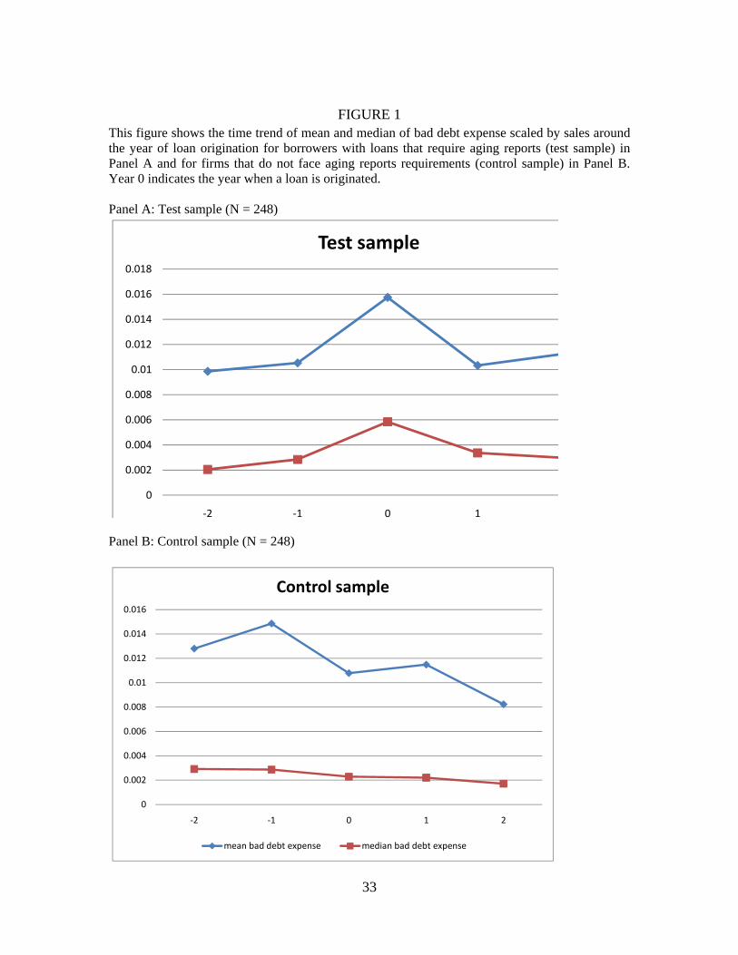
Figure 1 illustrates the change in the recognition of bad debt expense in the four

years around loan origination for both the borrowing sample and the matching sample.

The amount for the borrowing sample starts increasing in t-1, one year before loan

origination, suggesting that firms expecting to borrow from banks start to adjust their

accounting policy even before the borrowing. The amount increases sharply in the loan

21

origination year t, and remains at a level higher than that in the pre-borrowing period. In

contrast, the bad debt expense for the control sample drops in the year of loan origination

and this trend remains two years after loan origination, which could reflect overall

increases in credit quality in the customers of the industry. The univariate analysis and

the graph provide initial evidence supporting our hypothesis that firms report higher bad

debt expense given the requirement to provide an aging report to a bank.

[Insert Figure 1 Here]

The attenuated increase in ALLOW can be explained, in part, by the increases in

write-offs (WO) in the loan year. The increase in the write-offs can be either due to the

deteriorating collectability of receivables, which could cause firms simultaneously to

increase bad debt expenses and borrow from banks, or changes in accounting policy. The

second explanation assumes the decision to write-off an account involves discretion on

the part of the holder of the receivable and that active monitoring by banks can pressure

borrowers to write off questionable accounts.19 Under this explanation, the write-offs of

accounts receivables are not purely driven by the performance or the riskiness of

receivables and instead are subject to managers’ discretion. On the other hand, if write-

offs indicate future credit risk, a significant increase in write-offs after borrowings is

problematic for our empirical identification, because the increase can cause a spurious

correlation between a loan origination and an increase in bad debt expenses. Inspection

of the data indicates that the increase in write-offs occurs primarily year t and that write-

off in years t+1 and t+2 resemble pre-loan levels. This evidence suggests that the

increase in write-offs is a temporary phenomenon that coincides with the year of loan

19 This is particularly possible when banks impose a cross-aging requirement on borrowers. Under these circumstance a borrower would have an incentive to clear past due accounts out of the receivable ledger by writing them off.

22

initiation. In any event, these results suggest the necessity of controlling for future write-

offs as well as industry performance to distinguish accounting policy changes from credit

quality changes.

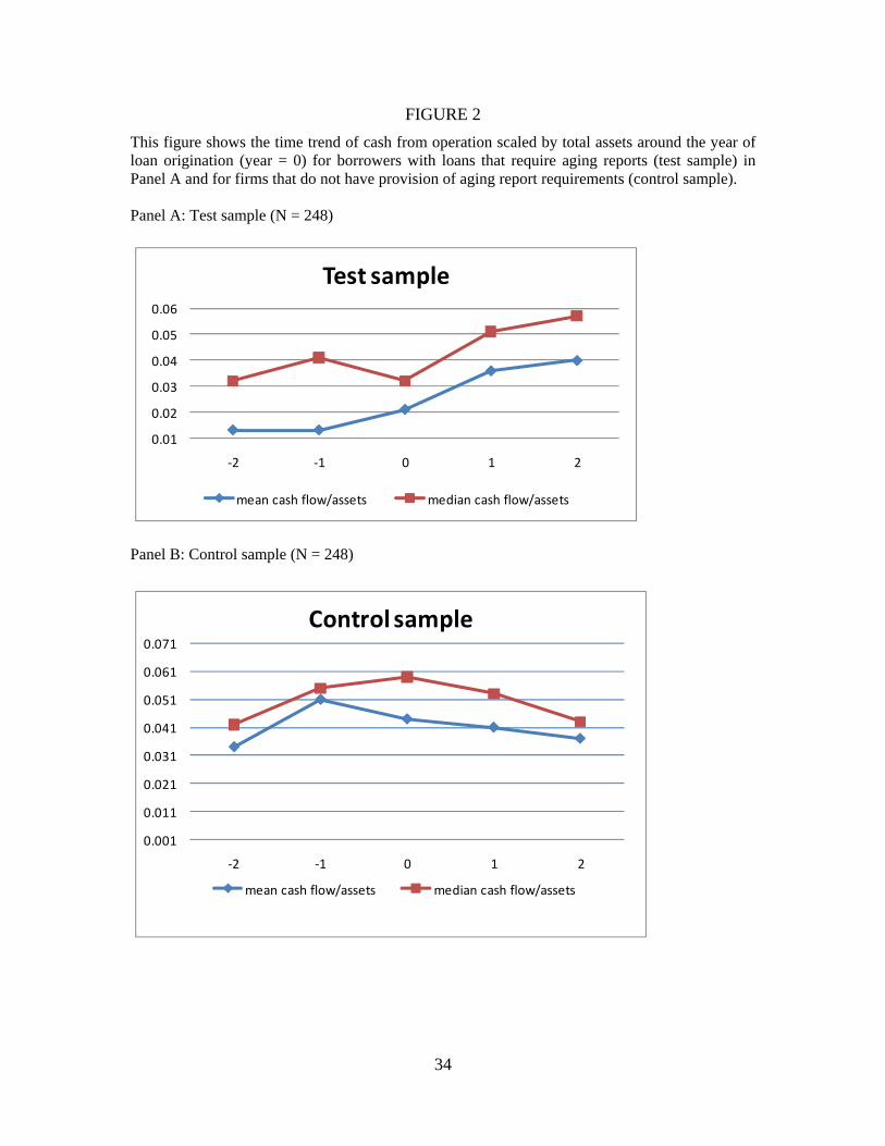
A firm’s performance is likely to be negatively affected by deteriorating credit

quality of its customers. We compare borrowing firms’ operating performance to that of

control firms. As shown in the table, cash flows from operations (CFO) increase

significantly during the post-period for sample firms. Figure 2 also illustrates this point.

The mean values of CFO increases monotonically from 0.013 in t-2 to 0.032 in t+1,

suggesting firms’ operating performances improved after loan origination rather than

deteriorated. This increase contrasts with the control sample whose CFO declines; though

Table 4 indicates this decline is moderate.

[Insert Figure 2 Here]

In addition, Table 4 shows that total asset turnovers (SALES) remain the same

after borrowing. Compared to the matching firms, borrowing firms have higher revenue,

are smaller in size and are less likely to be followed by analysts. At the industry level, all

the changes in the economic indicator variables point in the same direction—that the

industries that borrowing firms belong to experience an improvement in the economic

performance. For example, the median accounts receivable turnover ratio at the industry

level (ARTO_IND) increases significantly; both the standard deviation of sales

(SALES_SD_IND) and Altman z-score (ALT_IND) at the industry level decrease

significantly.

5. Multivariate Analyses

5.1. Main regression results

23

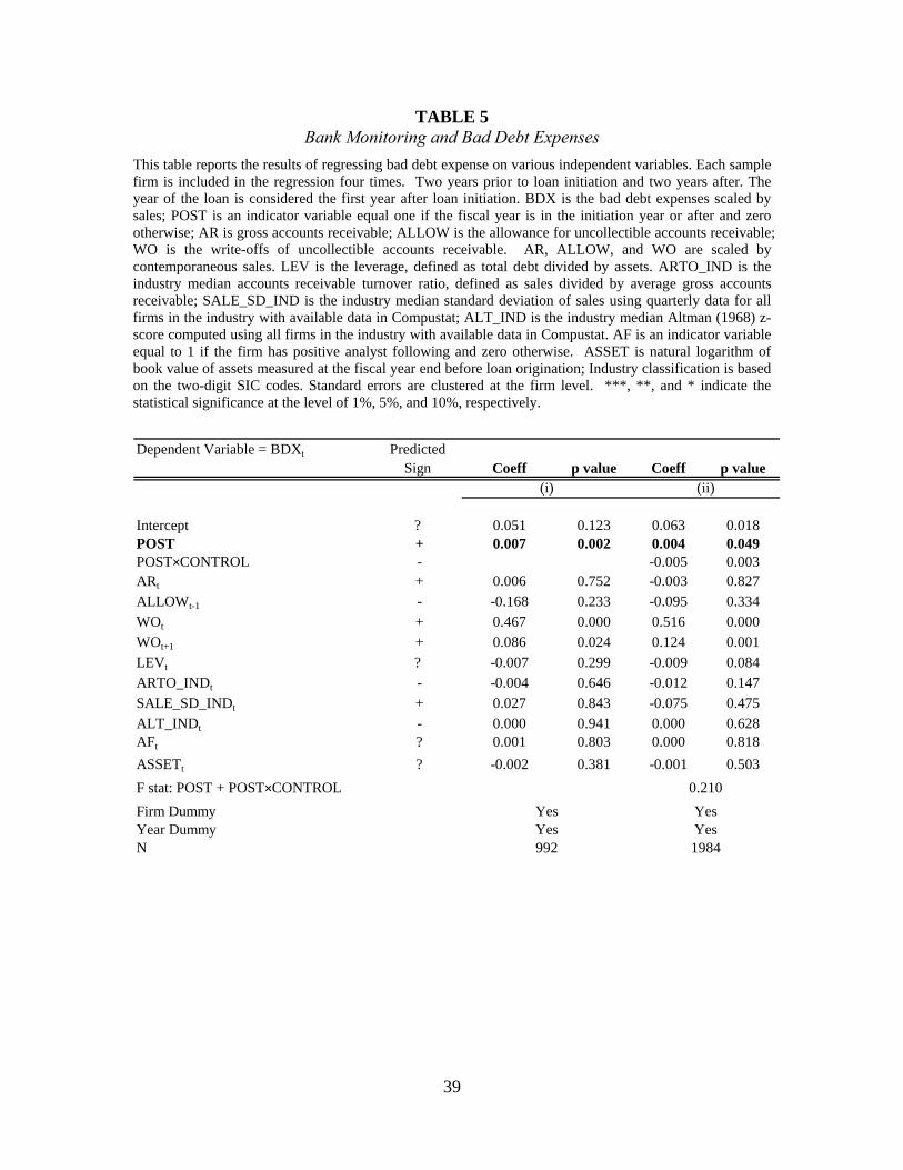
Table 5 reports the results of testing the effect of bank monitoring on the

recognition of bad debt expense for the test sample in column (i) and for the sample

containing both the test firms and the control firms in column (ii). The coefficient on

POST is positive and statistically significant in column (i), suggesting that after

borrowing, firms increase their bad debt expense significantly. In terms of magnitude,

borrowing firms experience an increase in bad debt expenses of 0.007 (0.7% of total

sales). The increase is also economically significant. The average of BDX in the period

before borrowings is 0.010 (1.0% of total sales), and a change of 0.7% of sales in bad

debt expenses represents a more than 50% increase. Given that the average sales are 542

million dollars, bad debt expenses increase by 3.8 million dollars after borrowing.

For the control variables, both current and next period’s write-offs of accounts

receivable are positively correlated with bad debt expenses, suggesting that firm’s bad

debt expense reflects expected credit quality of receivables. The coefficient on LEV is

negative but not significant (β6 = -0.007 with a p-value of 0.299), providing weak

evidence that managers tend to reduce bad debt expenses as debt increases. Further, the

coefficients on the three industry-wide economic factors all have predicted signs but are

not statistically significant. The adjusted R-Square is 79%, suggesting that the model

explains a significant portion of the variation in bad debt expenses, but this R-square also

reflects the explanatory power of firm and year fixed effects.

In column (ii), the coefficient on POST continues to be positive and statistically

significant at the .05 level. In contrast, the coefficient on the interaction between POST

and CONTROL is negative and statistically significant at the .01 level and an F test of the

sum of POST and POST×CONTROL is not statistically significant. These results suggest

24

that test firms recognize more bad debt expense after loan origination whereas this does

not occur to the matching firms. Therefore, the increase in bad debt expense recognition

for the borrowing firms is not significantly related to industry-wide effects. In sum, we

document a significant increase in bad debt expense recognition for firms that borrow

with an aging report requirement. We attribute this increase to bank monitoring of

borrowers’ accounts receivable.

[Insert Table 5]

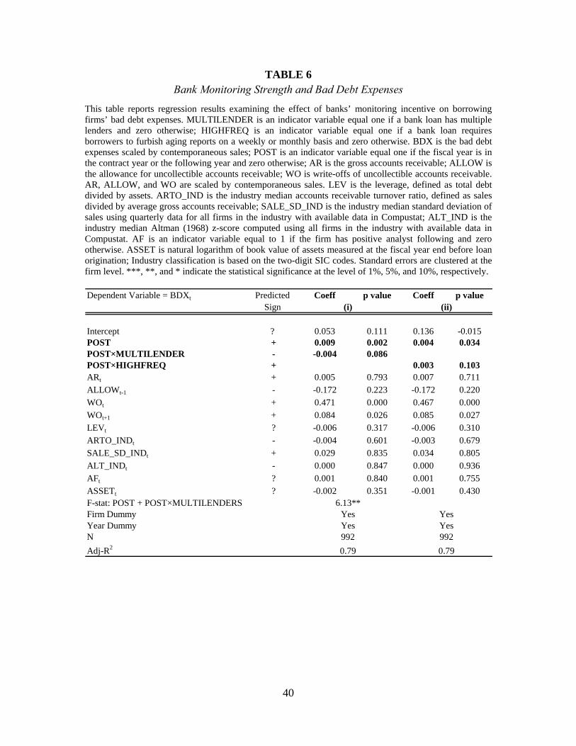
5.2 Cross-sectional analysis of bank monitoring incentive and intensity

In this section, we provide evidence on how the changes in bad debt expense vary

with banks’ monitoring intensity for our test sample. We expect that a bank’s monitoring

incentive is weaker when a loan has multiple lenders and a bank’s monitoring intensity is

stronger when a loan requires more frequent aging reports. Results presented in table 6

demonstrate that the increase in bad debt expense is lower for syndicated loans with

multiple lenders. As shown in column (i), the coefficient on POST × MULTILENDERS is

negative and statistically significant at the .10 level. Whereas firms with single-lender

loans increase their bad debt expenses by 0.009, the increase for firms with syndicated

loans is only 0.005 (0.009 – 0.004) and the F-statistic indicates that this increase remains

significant at the .05 level. Hence, the increase in bad debt expenses for borrowers with

single-lender loans is approximately twice that of borrowers with multiple-lender loans.

In column (ii) we examine whether the frequency of bank monitoring affects the

changes in bad debt expenses. The coefficient on POST * HIGHFREQ is positive and

marginally significant at the .10 level. The increase in bad debt expenses for firms with

low monitoring frequency (quarterly or longer, including upon request) is 0.004 after loan

25

origination. For firms with high frequency of aging reports (weekly or monthly), the

change in bad debt expense is 0.007 (0.004 + 0.003).

[Insert Table 6 Here]

5.3 Business conditions and bank monitoring

Bank monitoring incentives and therefore intensity can both change overtime. For

example, during weak economic conditions firms tend to perform poorly, resulting in

increased borrower credit risk and divergence between borrower and lender interests.

Bank vigilance can increase during such periods as lenders strive to protect their

investments prior to deterioration in the value of expected payments and collateral. If the

observed increase in bad debt expense results from bank monitoring, we expect a greater

increase when banks show heightened attention to covenants and credit standards.

We test this prediction using Senior Loan Officer Survey data from the Federal

Reserve.20 The Federal Reserve generally conducts quarterly surveys of senior loan

officers at approximately sixty large domestic banks and twenty-four U.S. branches and

agencies of foreign banks. Survey questions cover changes in the standards and terms of

the banks' lending and the state of business and household demand for loans. We focus

on loan officers’ response to the ‘loan terms’ question. The response has five levels

(tightened considerably, tightened somewhat, unchanged, eased somewhat, and eased

considerably).21 We compute an annual score, equal to the sum of quarterly scores. For

detailed description of the survey and the computation of the annual score, please refer to

20 We obtain Loan Officer Survey data from the Federal Reserve Board website at http://www.federalreserve.gov/boarddocs/SnLoanSurvey/. 21 The question reads as follows, “For applications for C&I (ed: commercial and industrial) loans or credit lines—other than those to be used to finance mergers and acquisitions—from large and middle-market firms and from small firms that your bank currently is willing to approve, how have the terms of those loans changed over the past three months?” We use responses related to larger borrowers (above $50M in sales) as these firms correspond to those in our tests.

26

Appendix A. We then partition our test sample into two subgroups based on the median

value of the annual score for loan covenant and run equation (1). We expect the

coefficient on POST to be greater in the tight period where the annual score is less than

11.845. Results are reported in Table 7. Indeed, we observe the coefficient of interest is

0.007 for the tight credit period and in contrast it is 0.002 in the loose credit period,

which is consistent with our expectation that increased recognition of bad debt expense

for borrowers after loan origination becomes more pronounced when banks are more alert

to financial distress.

[Insert Table 7 Here]

6. Robustness Check

6.1 Additional control variables

As shown in Table 3 firm size and the presence of analyst following are highly

correlated with multi-lender loans and the frequency of aging reports. Therefore their

interactions with POST can be a correlated omitted variable in our cross-sectional tests.

To address this concern we rerun regressions in Table 6 and include these two interaction

terms. Our results are robust to this procedure suggesting that other governance

mechanisms do not substitute the role of bank monitoring of borrowers’ accounts

receivable.

6.2 Scaling variables by accounts receivable or assets

All the results presented are based on scaling bad debt expense and other

independent variables by sales. To investigate whether our results are driven by the

choice of scaling factor, we replace sales with accounts receivable (and, alternatively,

book value of assets) as the scaling variable. The variable AR is removed from the

27

equation when receivables serves as the scaling variable, because including AR can cause

a mechanical negative association between the dependent variable and AR. Unreported

results show that our findings are not sensitive to the choice of scaling variable.

7. Conclusion

We study changes in accounting recognition related to accounts receivable

surrounding the initiation of loans requiring the provision of aging schedules to the lender.

We find that bad debt expense recognition increases significantly after loan initiation

controlling for write-offs, receivable turnover, the beginning allowance balance, and firm

and year fixed effects. This increase is more pronounced for loans characterized by

increased monitoring incentive and intensity, and during the periods of higher credit

standards. In addition, monitoring by security analysts does not substitute for this effect.

Our results provide direct confirmation of two widely held beliefs in banking and

accounting research. The first is that banks monitor firms. Such monitoring is thought to

be an important reason for the existence of banks. With some notable exceptions, prior

research provides indirect evidence of this monitoring by examining stock-price reactions

to bank loan announcements and by studying accruals before and after loans. The second

is that banks demand conservative accounting and that these demands affect firm

accounting policies. Our results suggest that banks’ influence is unique in that it is not

overwhelmed by other monitoring mechanisms in place.

28

APPENDIX Computation of Loan Officer Evaluation Score

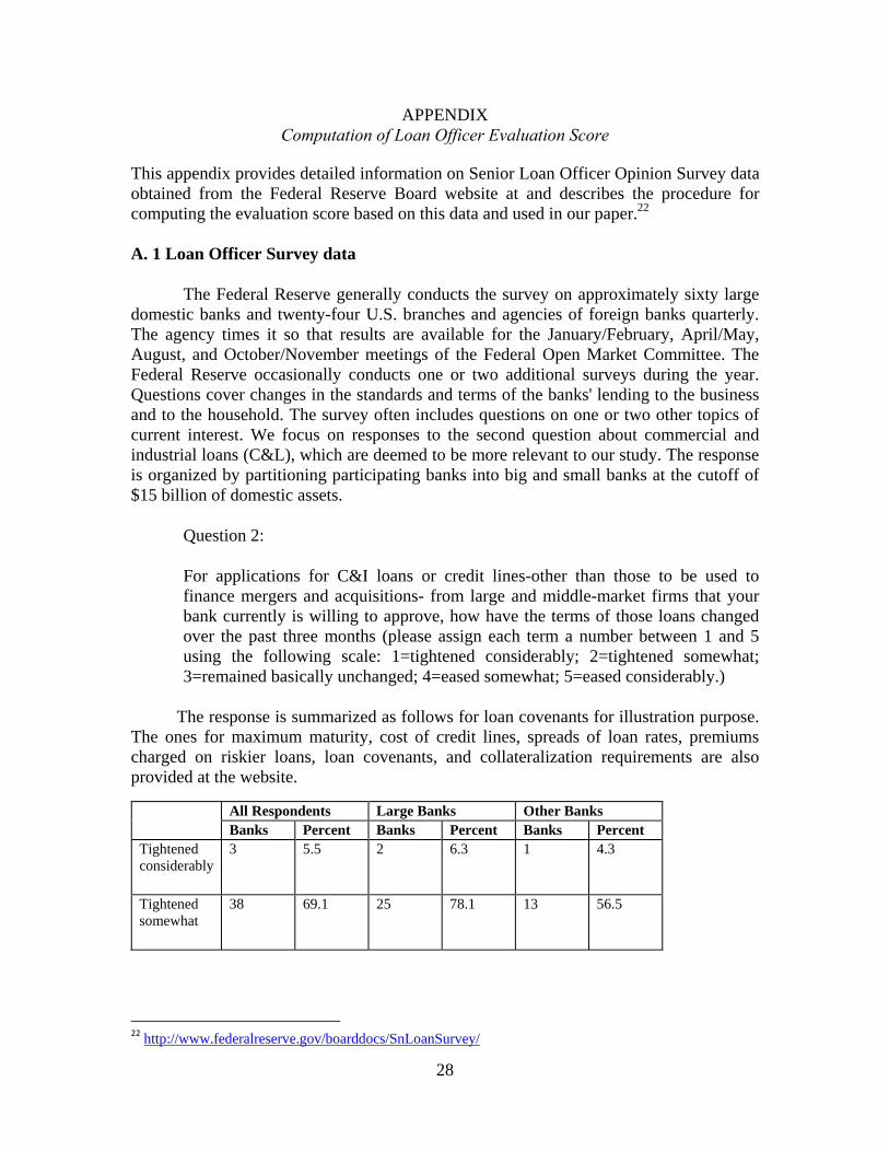
This appendix provides detailed information on Senior Loan Officer Opinion Survey data obtained from the Federal Reserve Board website at and describes the procedure for computing the evaluation score based on this data and used in our paper.22 A. 1 Loan Officer Survey data

The Federal Reserve generally conducts the survey on approximately sixty large domestic banks and twenty-four U.S. branches and agencies of foreign banks quarterly. The agency times it so that results are available for the January/February, April/May, August, and October/November meetings of the Federal Open Market Committee. The Federal Reserve occasionally conducts one or two additional surveys during the year. Questions cover changes in the standards and terms of the banks' lending to the business and to the household. The survey often includes questions on one or two other topics of current interest. We focus on responses to the second question about commercial and industrial loans (C&L), which are deemed to be more relevant to our study. The response is organized by partitioning participating banks into big and small banks at the cutoff of $15 billion of domestic assets.

Question 2:

For applications for C&I loans or credit lines-other than those to be used to finance mergers and acquisitions- from large and middle-market firms that your bank currently is willing to approve, how have the terms of those loans changed over the past three months (please assign each term a number between 1 and 5 using the following scale: 1=tightened considerably; 2=tightened somewhat; 3=remained basically unchanged; 4=eased somewhat; 5=eased considerably.)

The response is summarized as follows for loan covenants for illustration purpose. The ones for maximum maturity, cost of credit lines, spreads of loan rates, premiums charged on riskier loans, loan covenants, and collateralization requirements are also provided at the website.

All Respondents Large Banks Other Banks Banks Percent Banks Percent Banks Percent Tightened considerably

3 5.5 2 6.3 1 4.3

Tightened somewhat

38 69.1 25 78.1 13 56.5

22 http://www.federalreserve.gov/boarddocs/SnLoanSurvey/ 

29

Remained basically unchanged

14 25.5 5 15.6 9 39.1

Eased somewhat

0 0 0 0 0 0

Eased considerably

0 0 0 0 0 0

Total 55 100 32 100 23 100

A.2 Computation of loan officer evaluation score We compute the loan officer evaluation score for each surveyed quarter by multiplying

the level of response (1=tightened considerably; 2=tightened somewhat; 3=remained basically unchanged; 4=eased somewhat; 5=eased considerably) by the percentage of banks having this level of response first. Second, we sum it up across all levels of responses for both large banks and small banks for small borrowing firms only to arrive at a weighted -average response for each dimension of credit terms. We choose responses for small firms because our sample firms are relatively small. Third, we take the average of the weighted-average response score across big and small banks. Fourth, the quarterly score is summed to derive our annual measure of evaluation score for each dimension of credit terms.

In the regression, we use the annual score for loan covenant as the measure of credit market condition.

To gauge bank monitoring intensity that is orthogonal to borrowers’ credit risk, we use regression technique to regress loan covenant tightness on spreads of loan rates over base rates and obtain the residual of the regression as the measure of bank monitoring intensity. A higher level of the residual indicates a more favorable credit market condition for borrowers, thus lower bank monitoring intensity. The summary statistic for the seven dimensions of credit terms is as follows for the period 1997-2007.

Lower UpperN Mean Quartile Median Quartile Std Dev

COLLATERAL 11 11.700 11.250 11.920 12.030 0.477LOAN COVENANT 11 11.770 11.215 11.845 12.275 0.614PREMIUM RISK 10 10.339 10.045 11.170 12.030 2.796SPREADS 11 12.277 11.365 12.205 13.200 0.978COST OF CL 11 11.998 11.390 12.000 12.650 0.656MAX SIZE 11 11.957 11.705 11.985 12.190 0.384MAX MATURITY 3 11.237 9.430 11.937 12.345 1.578COMPOSITE SCORE 11 11.665 10.933 11.780 12.361 0.701RESIDUAL LOAN COVENANT 11 -0.072 -0.324 -0.036 0.053 0.215

 

 

 

30

REFERENCES AHMED, A. B., BILLINGS, R., MORTON, and M., STANFORD. ‘The Role of

Accounting Conservatism in Mitigating Bondholder-Shareholder Conflicts over Dividend Policy and in Reducing Debt Costs.’ The Accounting Review 77 (2002): 867-890.

AHN, S., and W. CHOI. ‘The Role of Bank Monitoring in Corporate Governance:

Evidence from Borrowers’ Earnings Management Behavior.’ Journal of Banking and Finance 33 (2009): 425 – 434.

BALL, R., S. P. KOTHARI, and A. ROBIN. ‘The Effect of International Institutional Factors

on Properties of Accounting Earnings.’ Journal of Accounting and Economics 29 (2000): 1-51.

BARNETT, W. ‘What’s In A Name? A Brief Overview of Asset-Based Lending.’ The Secured Lender 53(1997): 80-82

BEATTY, A., J. WEBER, and J. YU. ‘Conservatism and Debt.’ Journal of Accounting

and Economics 45 (2008): 154-174. BEST, R., and H. ZHANG. ‘Alternative Information Sources and The Information Content

of Bank Loans.’ Journal of Finance 4 (1993): 1507-1523.

BILLET, M., M. FLANNERY., and J. GARFINKEL. ‘Are Bank Loans Special? Evidence on The Post-Announcement Performance of Bank Borrowers.’ Journal of Financial and Quantitative Analysis 50 (2006): 733-751.

BOLTON, P., and D. SCHARFSTEIN. ‘A Theory of Predation Based on Agency Problem in Financial Contracting.’ The American Economic Review (1990): 93-106.

BUSHMAN, R., and R. WITTENBERG-MOERMAN. ‘The Role of Bank Reputation in “Certifying” Future Performance Implications of Borrowers’ Accounting Numbers.’ Working paper, University of North Carolina and University of Chicago, 2010.

DEANGELO, H., L. DEANGELO, and D. J. SKINNER. ‘Accounting Choice in Troubled Companies.’ Journal of Accounting and Economics 17 (1994): 113–43.

DEFOND, M., and J. JIAMBALVO. ‘Debt Covenant Violation and Manipulation of

Accruals’. Journal of Accounting and Economics 17 (1994), 145-176. DIAMOND, D. W. ‘Financial Intermediation and Delegated Monitoring.’ Review of

Economic Studies 51 (1984): 393-414. DICHEV, I., and D. SKINNER. ‘Large-Sample Evidence on The Debt Covenant

Hypothesis.’ Journal of Accounting Research 40 (2002): 1091–1123.

31

FAMA, E. ‘What’s Different About Banks?’ Journal of Monetary Economics 15 (1985): 29-39.

FLANNERY, M., and X. WANG. ‘Borrowing Base Revolvers: Liquidity for Risky Firms.’

Working Paper, University of Florida, 2011.

FRANKEL, R., and ROYCHOWDHURY, S., 2009, “Are all special items equally special? The predictive role of conservatism, Washington University working paper.

HEALY, PAUL M., and K. G. PALEPU. “Effectiveness of Accounting-Based Dividend

Covenants.” Journal of Accounting and Economics 12 (1990): 97–133. JACKSON, S. B., and X. LIU. ‘The Allowance For Uncollectible Accounts,

Conservatism, and Earnings Management.’ Journal of Accounting Research 48 (2010): 565-601.

JAMES, C. ‘Some Evidence of The Uniqueness of Bank Loans.’ Journal of financial

economics 19 (1987) : 217-235.

JIMENEZ, G., J. LOPEZ, and J. SAURINA. ‘Empirical Analysis of Corporate Credit Lines.’ Review of Financial Studies 22 (2009): 2059-5098.

KAHN, M., and R. WATTS, R. ‘Estimation And Empirical Properties of A Firm-Year

Measure of Accounting Conservatism.’ Journal of Accounting and Economics 48 (2009): 132-150.

KIM, B. H. ‘Ex-Post Change in Conservatism and Debt-Covenant Slack.’ working paper,

American University 2010 LAFOND, R., and R. WATTS. ‘The Information Role of Conservatism.’ The Accounting

Review 83 (2008): 447-478. LEFTWICH, R. ‘Accounting Information in Private Markets: Evidence From Private

Lending Agreements.’ Accounting Review 58 (1983): 23–42. LELAND, H., and D. PYLE. ‘Informational Asymmetries, Financial Structure, and

Financial Intermediation.’ Journal of Finance, 32 (1977): 371-415. LUMMER, S., and J. MCCONNELL. ‘Further Evidence on The Bank Lending Process and

The Capital Market Response to Bank Loan Agreements.’ Journal of Financial Economics 25 (1989): 99-122.

MCNICHOLS, M., and P. WILSON. ‘Evidence of Earnings Management from the Provision for Bad Debts.’ Journal of Accounting Research 26 (1988): 1–31.

32

MESTER, L. J., L. L. NAKAMURA, and M. RENAUT ‘Transactions Accounts And Loan Monitoring.’ Review of Financial Studies, 20 (2007), 529-556.

MIKKELSON, W., and M. PARTCH. ‘Valuation Effects of Securities Offerings and The

Issuance Process.’ Journal of Financial Economics 15 (1986): 31-60.

MOERMAN, M., R. ‘The Role of Information Asymmetry and Financial Reporting Quality in Debt Contracting: Evidence Form The Secondary Loan Market.’ Journal of Accounting and Economics 46 (2008): 240-260.

NIKOLAEV, V. ‘Debt Covenants and Accounting Conservatism.’ Journal of

Accounting Research 48 (2010): 137-175. NORDEN, L., and M., WEBER. ‘Credit Line Usage, Checking Account Activity, And

Default Risk of Bank Borrowers.’ Review of Financial Studies, 23 (2010): 3665-3699.

SWEENEY, A. ‘Debt-Covenant Violations and Managers’ Accounting Responses.’

Journal of Accounting and Economics 17 (1994): 281–308. SUFI, A. ‘Bank Line of Credit in Corporate Finance: An Empirical Analysis.’ Review of

Financial Studies 22 (2009): 1057-1088.

TAN, L. ‘Creditor Control, State of Nature Verification, and Financial Reporting Conservatism.’ Working paper, Northwestern University, 2011.

WATTS, R. ‘Conservatism in Accounting, Part I: Explanations and Implications.’ Accounting Horizons 17 (2003): 207–221.

WATTS, R., and J. ZIMMERMAN. Positive Accounting Theory. Prentice-Hall,

Englewood Cliffs, NJ, 1986.Englewood Cliffs, NJ, 1986. ZHANG, J. ‘The Contracting Benefits of Accounting Conservatism to Lenders and

Borrowers.’ Journal of Accounting and Economics 45 (2008): 27-54.

33

FIGURE 1

This figure shows the time trend of mean and median of bad debt expense scaled by sales around the year of loan origination for borrowers with loans that require aging reports (test sample) in Panel A and for firms that do not face aging reports requirements (control sample) in Panel B. Year 0 indicates the year when a loan is originated. Panel A: Test sample (N = 248)

0

0.002

0.004

0.006

0.008

0.01

0.012

0.014

0.016

0.018

‐2 ‐1 0 1

Test sample

Panel B: Control sample (N = 248)

0

0.002

0.004

0.006

0.008

0.01

0.012

0.014

0.016

‐2 ‐1 0 1 2

Control sample

mean bad debt expense median bad debt expense

34

FIGURE 2

This figure shows the time trend of cash from operation scaled by total assets around the year of loan origination (year = 0) for borrowers with loans that require aging reports (test sample) in Panel A and for firms that do not have provision of aging report requirements (control sample). Panel A: Test sample (N = 248)

0.01

0.02

0.03

0.04

0.05

0.06

‐2 ‐1 0 1 2

Test sample

mean cash flow/assets median cash flow/assets

Panel B: Control sample (N = 248)

0.001

0.011

0.021

0.031

0.041

0.051

0.061

0.071

‐2 ‐1 0 1 2

Control sample

mean cash flow/assets median cash flow/assets

35

TABLE 1 Time and Industry Profile of Sample

This table describes the yearly distribution of our sample of borrowers with loans that require aging reports in Panel A and its industry profile in Panel B. Panel A: Time profile of sample

year Frequency Percentage Year Frequency Pecentage

1994 4 1.60% 2001 42 16.80%

1995 12 4.80% 2002 19 7.60%

1996 23 9.20% 2003 7 2.80%

1997 23 9.20% 2004 8 3.20%

1998 31 12.40% 2005 8 3.20%

1999 27 10.80% 2006 6 2.40%

2000 40 16.00%

Panel B: Industry profile of sample

Industry FrequencyFrequency Persentage

FrequencyFrequency Percentage

Agriculture, Forestry, &Fishing 0 0.0% 57 0.3%

Mining 6 2.4% 1,183 6.7%

Construction 2 0.8% 162 0.9%

Manufacturing 134 54.0% 6,073 34.5%

Transportation & Public Utilities 5 2.0% 1,610 9.1%

Wholesale Trade 16 6.5% 539 3.1%

Retail Trade 8 3.2% 900 5.1%

Finance, Insurance, &Real Estate 2 0.8% 3,801 21.6%

Services 75 30.2% 3,068 17.4%

Nonclassifiable Establishments 0 0.0% 217 1.2%

Total 248 100.0% 17,608 100.0%

Sample Firms Compustat Universe Firms

36

TABLE 2 Characteristics of Loan Contracts with Aging Report Requirements

This table presents loan characteristics in Panel A, the purpose of aging reports in Panel B, and the frequency of aging reports in Panel C. LOAN_AMOUNT is the size of a loan in millions of dollars; MATURITY is the maturity of a loan in years; MULTILENDERS is a indicator variable equal to one for a syndicated loan with multiple lenders and zero otherwise; CUTOFF_INVOICE is the maximum number of days following the invoice date allowable for a customer receivable to be included as eligible accounts receivable in the computation of the borrowing base; CUTOFF_DUE is the maximum number of days following the due date of the invoice for a customer accounts receivable to be included in the computation of the borrowing base; PCT_BASE is the percentage of eligible accounts receivable used as the borrowing base.

Lower Upper

N Mean Quartile Median Quartile Std Dev

LOAN AMOUNT 242 52.712 18.000 18.000 50.000 102.262

MATURITY 242 2.790 2.000 3.000 3.500 1.434

MULTILENDERS 248 0.508 0.000 1.000 1.000 0.501

CUTOFF_INVOICE 170 104.612 90.000 90.000 120.000 29.000

CUTOFF_DUE 67 69.701 60.000 60.000 90.000 18.152

PCT_BASE 179 81.778 80.000 80.000 85.000 6.555

Panel A. Loan characteristics

Purpose Frequency

Borrowing Base Only 66

Collateral Only 40

Borrowing Base and Collateral

113

Other 29

Total 248

Panel B: Purpose of aging report

Panel C. Frequency of aging reportsFrequency Number Percentage

Weekly 4 1.6%

Monthly 164 66.1%

Quarterly 39 15.7%

Semi-Annually 2 0.8%

Annually 6 2.4%

By Request 33 13.3%

Total 248 100%

37

TABLE 3 Correlation between Variables

This table reports Pearson correlation below the diagonal and Spearman correlation above the diagonal for the test sample. A firm is included in the test sample when a loan contract when required aging reports can be identified. Firm characteristics are measured at the fiscal-year end immediately prior to the loan origination year. BDX is bad debt expenses scaled by contemporaneous sales; LEV is leverage, defined as total debt (long-term and short-term) divided by assets. CFO is cash flow from operation scaled by assets; ASSET is natural logarithm of book value of assets; AF is an indicator variable equal to 1 if the firm has positive analyst following and zero otherwise. MULTILENDER is an indicator variable equal one if a bank loan has multiple lenders and zero otherwise; HIGHFREQ is an indicator variable equal one if a bank loan requires borrowers to furbish aging reports on a weekly or monthly basis and zero otherwise. RETVOL is the variance of monthly returns. Correlations with significance 5% (two-tailed) are in bold.

Variable BDX RETVOL ROA CFO ASSETS LEVERAGE AFMULTILEN

DERHIGHFREQ

BDX 0.168 -0.196 -0.058 -0.022 0.061 -0.064 0.019 -0.014RETVOL 0.168 -0.318 -0.192 -0.174 -0.044 -0.118 -0.084 0.070ROA -0.228 -0.354 0.401 0.063 -0.172 0.187 0.009 -0.064CFO -0.158 -0.254 0.470 0.171 -0.060 0.145 0.114 -0.109ASSET -0.017 -0.185 0.152 0.218 0.297 0.357 0.585 -0.188LEV 0.129 0.048 -0.021 -0.043 0.272 -0.054 0.252 -0.028AF -0.137 -0.141 0.173 0.148 0.345 -0.080 0.141 -0.060MULTILENDER 0.003 -0.082 0.051 0.130 0.552 0.241 0.141 -0.108HIGHFREQ 0.045 0.075 -0.070 -0.095 -0.197 -0.027 -0.060 -0.108

38

TABLE 4 Firm Characteristics before and after the Loan Initiation

This table reports mean statistics for firm characteristics in the two years before and two years (after and including) the year of loan initiation for both the test sample and the control sample. BDX is bad debt expenses; AR is the gross accounts receivable; ALLOW is the allowance for uncollectible accounts receivable; WO is the write-offs of uncollectible accounts receivable. BDX, AR, ALLOW, and WO are scaled by contemporaneous sales. LEV is leverage, defined as total debt (long-term and short-term) divided by assets. SALES is total sales scaled by assets; CFO is cash flow from operation scaled by assets; ASSET is natural logarithm of book value of assets measured at the fiscal year end before loan origination; ‘No. Ana Follow’ is the number of analysts following the borrower. ARTO_IND is industry median accounts receivable turnover ratio, defined as sales divided by average gross accounts receivable; SALE_SD_IND is industry median standard deviation of sales using quarterly data for all firms in the same industry with available data in Compustat; ALT_IND is industry median Altman (1968) z-score computed using all firms in the industry with available data in Compustat. Industry classification is based on two-digit SIC codes. ***, **, and * indicate the statistical significance for the difference of the mean values at the level of 1%, 5%, and 10%, respectively.

Pre Post Pre Post (2) - (1) (4) - (3) (1) - (3) (2) - (4)

(1) (2) (3) (4) (5) (6) (7) (8)

BDX 0.010 0.012 0.014 0.010 0.002** -0.004*** -0.004 0.002

AR 0.191 0.179 0.185 0.169 -0.012** -0.016*** 0.006 0.010**

ALLOW 0.013 0.015 0.016 0.016 0.002 0.000 -0.003 0.001

WO 0.012 0.016 0.013 0.013 0.004*** 0.000 -0.001 0.003

LEV 0.252 0.267 0.250 0.244 0.015 -0.006 0.002 0.023

SALES 1.576 1.543 1.270 1.237 -0.033 -0.033 0.306*** 0.306***

ROA -0.027 -0.065 -0.032 -0.035 -0.038*** -0.003 0.005 -0.030*

CFO 0.013 0.032 0.043 0.041 0.019** -0.002 -0.029** -0.009

ASSET 4.559 4.842 5.355 5.509 0.283*** 0.154*** -0.796*** 0.667***

No. Ana Follow 2.237 2.332 4.528 4.463 0.095 -0.065 -2.291*** -2.131***

ARTO_IND 1.974 2.014 1.974 2.014 0.040*** 0.040***

SALES_SD_IND 0.033 0.031 0.033 0.031 -0.002*** -0.002***

ALT_IND 3.248 2.821 3.248 2.821 -0.427*** -0.427***

Panel A: Descriptive statisticsTest sample Control sample Mean Diff.

39

TABLE 5 Bank Monitoring and Bad Debt Expenses

This table reports the results of regressing bad debt expense on various independent variables. Each sample firm is included in the regression four times. Two years prior to loan initiation and two years after. The year of the loan is considered the first year after loan initiation. BDX is the bad debt expenses scaled by sales; POST is an indicator variable equal one if the fiscal year is in the initiation year or after and zero otherwise; AR is gross accounts receivable; ALLOW is the allowance for uncollectible accounts receivable; WO is the write-offs of uncollectible accounts receivable. AR, ALLOW, and WO are scaled by contemporaneous sales. LEV is the leverage, defined as total debt divided by assets. ARTO_IND is the industry median accounts receivable turnover ratio, defined as sales divided by average gross accounts receivable; SALE_SD_IND is the industry median standard deviation of sales using quarterly data for all firms in the industry with available data in Compustat; ALT_IND is the industry median Altman (1968) z-score computed using all firms in the industry with available data in Compustat. AF is an indicator variable equal to 1 if the firm has positive analyst following and zero otherwise. ASSET is natural logarithm of book value of assets measured at the fiscal year end before loan origination; Industry classification is based on the two-digit SIC codes. Standard errors are clustered at the firm level. ***, **, and * indicate the statistical significance at the level of 1%, 5%, and 10%, respectively.

Dependent Variable = BDXt PredictedSign Coeff p value Coeff p value

Intercept ? 0.051 0.123 0.063 0.018POST + 0.007 0.002 0.004 0.049POST×CONTROL - -0.005 0.003ARt + 0.006 0.752 -0.003 0.827ALLOWt-1 - -0.168 0.233 -0.095 0.334

WOt + 0.467 0.000 0.516 0.000WOt+1 + 0.086 0.024 0.124 0.001

LEVt ? -0.007 0.299 -0.009 0.084ARTO_INDt - -0.004 0.646 -0.012 0.147

SALE_SD_INDt + 0.027 0.843 -0.075 0.475ALT_INDt - 0.000 0.941 0.000 0.628AFt ? 0.001 0.803 0.000 0.818

ASSETt ? -0.002 0.381 -0.001 0.503

F stat: POST + POST×CONTROL

Firm DummyYear DummyN

YesYes1984

0.210

(i) (ii)

YesYes992

40

TABLE 6 Bank Monitoring Strength and Bad Debt Expenses

This table reports regression results examining the effect of banks’ monitoring incentive on borrowing firms’ bad debt expenses. MULTILENDER is an indicator variable equal one if a bank loan has multiple lenders and zero otherwise; HIGHFREQ is an indicator variable equal one if a bank loan requires borrowers to furbish aging reports on a weekly or monthly basis and zero otherwise. BDX is the bad debt expenses scaled by contemporaneous sales; POST is an indicator variable equal one if the fiscal year is in the contract year or the following year and zero otherwise; AR is the gross accounts receivable; ALLOW is the allowance for uncollectible accounts receivable; WO is write-offs of uncollectible accounts receivable. AR, ALLOW, and WO are scaled by contemporaneous sales. LEV is the leverage, defined as total debt divided by assets. ARTO_IND is the industry median accounts receivable turnover ratio, defined as sales divided by average gross accounts receivable; SALE_SD_IND is the industry median standard deviation of sales using quarterly data for all firms in the industry with available data in Compustat; ALT_IND is the industry median Altman (1968) z-score computed using all firms in the industry with available data in Compustat. AF is an indicator variable equal to 1 if the firm has positive analyst following and zero otherwise. ASSET is natural logarithm of book value of assets measured at the fiscal year end before loan origination; Industry classification is based on the two-digit SIC codes. Standard errors are clustered at the firm level. ***, **, and * indicate the statistical significance at the level of 1%, 5%, and 10%, respectively. Dependent Variable = BDXt Predicted Coeff p value Coeff p value

Sign

Intercept ? 0.053 0.111 0.136 -0.015POST + 0.009 0.002 0.004 0.034POST×MULTILENDER - -0.004 0.086POST×HIGHFREQ + 0.003 0.103ARt + 0.005 0.793 0.007 0.711ALLOWt-1 - -0.172 0.223 -0.172 0.220

WOt + 0.471 0.000 0.467 0.000

WOt+1 + 0.084 0.026 0.085 0.027LEVt ? -0.006 0.317 -0.006 0.310

ARTO_INDt - -0.004 0.601 -0.003 0.679SALE_SD_INDt + 0.029 0.835 0.034 0.805

ALT_INDt - 0.000 0.847 0.000 0.936

AFt ? 0.001 0.840 0.001 0.755ASSETt ? -0.002 0.351 -0.001 0.430F-stat: POST + POST×MULTILENDERSFirm DummyYear DummyN

Adj-R2 0.79 0.79

Yes YesYes Yes

6.13**

(i) (ii)

992 992

41

TABLE 7

Business Condition and Bad Debt Expenses

This table reports regression results of examining the effect of business condition on bank monitoring of borrowing firms’ bad debt expenses. Tight credit market is defined as loan officer evaluation score for loan covenant above the median (11.845) during the period 1997 -2007. Loan officer evaluation score is discussed in Appendix B based on quarterly loan officer survey on seven dimensions obtained from Federal Reserve website; POST is a indicator variable equal one if the fiscal year is in the contract year or the following year after and zero otherwise; ALLOW is the allowance for uncollectible accounts receivable; WO is the write-offs of uncollectible accounts receivable. AR, ALLOW, and WO are scaled by contemporaneous sales. LEV is the leverage, defined as total debt divided by asset. ARTO_IND is the industry median accounts receivable turnover ratio, defined as sales divided by average gross accounts receivable; SALE_SD_IND is the industry median standard deviation of sales using quarterly data for all firms in the industry with available data in Compustat; ALT_IND is the industry median Altman (1968) z-score computed using all firms in the industry with available data in Compustat. ASSET is natural logarithm of book value of assets measured at the fiscal year end before loan origination; Industry classification is based on the two-digit SIC codes. Standard errors are clustered at the firm level. ***, **, and * indicate the statistical significance at the level of 1%, 5%, and 10%, respectively. Dependent Variable = BDXt Predicted

Sign Coeff p value Coeff p value

Intercept ? -0.004 0.907 0.049 0.432POST + 0.008 0.024 0.005 0.152ARt + 0.018 0.470 0.003 0.868

ALLOWt-1 - -0.114 0.540 -0.857 0.000WOt + 0.551 0.000 0.407 0.084

WOt+1 + 0.188 0.376 0.096 0.483LEVt ? -0.013 0.186 0.006 0.449

ARTO_INDt - -0.001 0.950 -0.012 0.581

SALE_SD_INDt + 0.134 0.392 -0.224 0.628ALT_INDt - 0.000 0.867 0.001 0.625

AFt ? 0.002 0.546 0.004 0.511ASSETt ? 0.001 0.743 -0.003 0.311Firm DummyYear DummyN

Adj-R2

Tight Credit Market (<=11.845) Loose Credit Market (>11.845)

500

0.79

YesYes

YesYes321

0.90