Bank Loan Price Reactions to Corporate Events: Evidence ... Loan Price Reactions to... · Bank Loan...

Bank Loan Price Reactions to Corporate Events: Evidence from Traded Syndicated Loans

Matthew T. Billett Kelley School of Business

Indiana University Department of Finance

1309 E 10th Street Bloomington, IN 47405 [email protected]

Redouane Elkamhi

Rotman School of Management University of Toronto 105 St. George Street

Toronto, Ontario, Canada M5S3E6 [email protected]

David C. Mauer

Belk College of Business University of North Carolina at Charlotte

9201 University City Blvd. Charlotte, NC 28223 [email protected]

Raunaq S. Pungaliya

SKK Graduate School of Business International Hall, Suite 339

25-2 Sungkyunkwan-ro, Jongno-gu Seoul, Korea 110-745

[email protected]

Current version: June, 2015

Bank Loan Price Reactions to Corporate Events: Evidence from Traded Syndicated Loans

Abstract

We study the influence of financial contracting on conflicts between equity holders and creditors by examining the reaction of bank loans to open market share repurchases. Since a share repurchase dilutes the claim of outstanding debt, the increase in the market value of equity at announcement may reflect a wealth transfer from creditors. In a sample of firms with traded loans, we find that the dollar return to equity at the announcement of an open market share repurchase increases by about 75 cents for every dollar lost in loan value. Consistent with theory, we find that senior bank debt in conjunction with a larger amount of junior non-bank debt attenuates the wealth transfer from debt holders to equity holders. Creditor monitoring through loan covenants suggests that a mix of incurrence and maintenance covenants also mitigates the negative impact of share repurchase on loan prices. JEL classification: G14, G24, M41 Keywords: Financial contracting, Traded loans, Open market share repurchase

1

1. Introduction

Event studies documenting wealth effects to security holders resulting from corporate

financing and investment decisions provide abundant evidence of value creation and destruction

and thereby provide an excellent laboratory to investigate how financial contracting mitigates

agency conflicts. Given the necessity of market prices to compute security holder wealth effects,

studies have not examined the impact of corporate events on bank loans which are one of the

largest sources of debt finance.1 On the one hand, we might not expect bank loans to exhibit

significant wealth effects given their short maturity, high priority, security, and typically rich set

of covenant restrictions. On the other hand, however, loans have these contractual features because

bank dependent borrowers face particularly high agency costs due to asymmetric information and

moral hazard.2 Using a new data set on secondary market loan prices, we examine the impact of

corporate events on loan value and the effect of debt priority structure and loan covenants on

wealth transfers between equity holders and creditors.

Our empirical analysis focuses on open market share repurchases because they are

significant corporate events that have the potential to dilute the claims of existing creditors since

shares are repurchased by selling corporate assets or issuing additional debt.3 We first ask whether

traded bank loan prices decrease at announcement of share repurchases and whether there is

evidence of a wealth transfer between loans and equity. We then examine whether financial

contracting mitigates the loss in loan value and any associated wealth transfer to equity. Our

analysis focuses on debt priority structure and loan covenants. In particular, we ask whether the

mix of bank debt and junior non-bank debt and the types of covenants in bank loans can attenuate

the impact of share repurchase on loan value.

1 Colla, Ippolito, and Li (2013) find that bank credit lines and term loans are the most commonly employed debt type after senior bonds and notes. 2 For example, see Diamond (1984, 1989, 1991, 1993), Rajan (1992), Chemmanur and Fulghieri (1994), Bolton and Freixas (2000), and Park (2000). See also Roberts and Sufi (2009) and Graham and Leary (2011) for recent surveys of the voluminous financial contracting and empirical capital structure literature. 3 We also examine the influence of seasoned equity issues on loan prices.

2

We examine the effect of open market share repurchase (OMR) announcements on bank

loan prices using a new data set on secondary market trading in the syndicated loan market. This

is a growing segment of the debt market with over $605 billion loans issued in 2013. Loan

syndicators are especially attracted to below investment grade borrowers because the fees for

arranging the loans are larger and because the higher spreads on “leveraged loans” are attractive

to investors. The most actively traded loans fund mergers and acquisitions (e.g., leveraged

buyouts), leveraged recapitalizations, and investment projects. In addition to banks, participants in

this market include pension funds, mutual funds, and hedge funds.

In a sample of OMRs during the period 2002 to 2012, we find a statistically and

economically significant negative effect of OMR announcements on loan prices. We further

document that shareholder wealth increases with losses to loans. Specifically, the equity dollar

return increases by about 75 cents for every dollar lost by loan holders. Overall, these results are

consistent with a strong wealth transfer from bank loan holders to equity holders in OMRs.

Theory suggests that banks are effective monitors, and their monitoring activity can

mitigate equity holder incentives to expropriate wealth from creditors (Diamond (1984, 1991,

1993), Bolton and Freixas (2000), Park (2000), DeMarzo and Sannikov (2006), and DeMarzo and

Fishman (2007)). Since on average banks appear to have incurred substantial losses at the

announcement of open market repurchases, an important question is whether certain characteristics

of the bank-borrower relationship, the loan contract, or the capital structure of the firm can explain

variability in loan losses. Consistent with the view that the bank-borrower relationship is important

(Boot (2000) and Ongena and Smith (2000)), we find that the length of the bank-borrower

relationship mitigates the negative effect of an OMR on loan returns. We also find that loan losses

at the announcement of an OMR are mitigated when the loan is backed by more collateral. In

contrast, however, we find that loan wealth effects are more negative as covenant intensity

increases, where following Bradley and Roberts (2004) and Demiroglu and James (2010) covenant

intensity is an index of incurrence covenants (e.g., dividend payment restriction) and maintenance

covenants (e.g., financial ratio restrictions tested quarterly). The negative relation between loan

3

returns and covenant intensity is consistent with a selection effect where loans that are more at risk

to potential agency conflicts – like the dilutive effect of an OMR – have more covenants. Indeed,

using Ivashina and Sun’s (2011) time on the market measure (TOM) to gauge the frothiness of the

syndicated loan market when the loan is issued – and therefore the likelihood of higher risk loans

coming to market – we find that TOM is negatively related to covenant intensity and positively

related to loan abnormal returns.4

Separating the covenant intensity index into incurrence covenants and maintenance

covenants sheds additional light on loan reactions to OMR announcements. In particular, we find

that incurrence covenants which are tested on the occurrence of an event, such as a restriction on

the payment of a dividend, have a negative effect on loan returns while maintenance covenants

which are checked at regular time intervals, such as financial ratio tests, have a positive effect on

loan returns. Furthermore, we find that having both incurrence and maintenance covenants has a

positive effect on a loan’s reaction to an OMR announcement. These results suggest that when

incurrence covenants fail to restrict a repurchase, the severity of loan holder wealth effects is

attenuated by the existence of maintenance covenants.

Another key result is that the debt structure of the firm significantly influences loan wealth

effects and the transfer of wealth from loan holders to equity holders. Park (2000) shows that moral

hazard problems between equity holders and creditors can be mitigated if a bank has the proper

incentives to monitor. To maximize the bank’s monitoring incentives, he establishes that the bank

loan should be senior and the amount of senior bank debt should be smaller than the amount of

junior non-bank debt.5 Since bank debt is explicitly or implicitly senior, we test the Park (2000)

model by examining whether the ratio of bank to total firm debt influences the loan price impact

4 Time on the market (TOM) is the number of days that it takes to sell the loan in the market, which is computed as the difference between the date that investors can begin to subscribe to the loan and the date the loan is fully funded. Ivashina and Sun (2011) argue that a shorter TOM indicates higher institutional demand and a frothier market. 5 See Park (2000, p. 2159) for the intuition for why the bank’s claim must be smaller than the claims of junior non-bank debt. See also Rauh and Sufi (2010, pp. 4255-4258) for an excellent discussion of the Park (2000) model and related literature.

4

of the OMR announcement.6 Consistent with Park (2000), we find that loan abnormal returns are

more negative the larger is the ratio of bank debt to total firm debt. We also find that the transfer

of wealth from loan holders to equity holders is increasing in the bank debt ratio. Overall, we find

considerable evidence that a firm’ priority structure and the amount of bank debt in the priority

structure influence the costs resulting from stockholder-bondholder agency conflicts.

As a parallel to open market repurchases, we examine loan wealth effects around seasoned

equity offerings (SEOs). We find that negative abnormal returns to equity holders at SEO

announcements are accompanied by positive abnormal returns to loans. In terms of wealth

transfers, we find that equity holders lose 25 cents for every dollar gained by loan holders. This

result is striking for several reasons. First, in the context of corporate bonds, Elliot, Prevost, and

Rao (2009) find no evidence of wealth transfers around SEOs.7 Second, loans should have limited

upside potential since that have short maturity and their price is pegged at par, and the majority of

loans can be prepaid early without penalty. Lastly, since the decision to issue equity is presumably

made to maximize the market value of equity, the firm would not want to raise equity capital if it

transfers significant wealth from equity holders to loan holders.

Our findings contrast with prior studies that examine bond holder wealth effects in OMRs.

Maxwell and Stephens (2003) report positive abnormal stock price reactions and negative

abnormal bond price reactions to the announcement of an OMR but they do not examine the

relation between stock and bond returns.8 Jun, Jung, and Walkling (2009) find similar stock and

bond price reactions but find no evidence that wealth changes to bond holders are inversely related

6 The senior bank debt and junior bonds priority structure studied in Park (2000) encourages bank monitoring of the firm to avert project selection that harms creditors. Our empirical analysis, however, is explicitly ex post (i.e., after an OMR that may dilute the claims of creditors). We therefore assume that a firm with a Park (2000) priority structure – relatively small amount of senior bank debt in a firm’s capital structure – would not undertake an OMR if it results in a significant wealth transfer from creditors to equity holders. 7 Although Elliot, Prevost, and Rao (2009) find positive bond holder reactions to SEO announcements, they find no evidence that bond holder and equity holder reactions are inversely related. In an earlier study, Kalay and Shimrat (1987) find negative bond holder reactions to SEO announcements. Eberhart and Siddique (2002) examine long-run returns to bond holders and equity holders after SEOs. They find positive long-run returns to bonds and negative long-run returns to stocks. 8 Evidence of a positive average stock price reaction and a negative average bond price reaction does not prove (or even imply) an inverse relation between stock and bond price reactions to OMRs (i.e., a wealth transfer).

5

to wealth changes to equity holders which is a necessary condition for wealth transfer. Indeed, in

their overall sample, Jun, Jung, and Walkling (2009) find a positive correlation between wealth

changes to stock holders and bond holders.

Our paper makes several contributions to the literature. First, it is the first paper to

demonstrate that wealth transfers (and hence agency conflicts) are significant in private debt

agreements. This is important because it is widely believed that loans are largely insulated from

corporate events since they have high priority, short maturity, and are typically secured. Second,

we document that financial contracting attenuates the negative wealth effect of harmful

transactions on debt prices. Specifically, we find that the bank-borrower relationship, the mix of

loan covenant types, and the relative amount of senior bank debt and junior bonds significantly

influences the reaction of loans to open market repurchases. Third, we are the first to use

syndicated loan prices to examine the response of private debt instruments to corporate events. As

described below, we develop a methodology to compute excess loan returns that confronts several

issues including accounting for infrequent trading and stale quotes and benchmarking loan returns.

The remainder of the paper proceeds as follows. The next section describes the data, the

methodology to compute abnormal loan returns, and presents summary statistics. Section 3 shows

the reaction of loans to open market share repurchases and examines how borrower and loan

characteristics influence loan price reactions. This section also documents wealth transfers

between loans and equity and examines the attenuating effects of priority structure. Section 4

examines loan returns around seasoned equity issues, and Section 5 concludes.

2. Data and Methodology

2.1. Data

Our sample selection process starts with all open market share repurchases (OMRs) and

seasoned equity offerings (SEOs) reported in the Securities Data Company (SDC) database during

the period 2002 to 2012. The sample begins in 2002 because this is the first year that we have data

on secondary market syndicated loan prices from the Thomson Reuters Loan Pricing Corporation

6

(LPC) database. Since we are interested in computing a loan’s price reaction to both OMR and

SEO events, we exclude firms that do not have at least one loan with valid data in the LPC database.

We further exclude firms in the financial and utility industries and any OMR (SEO) that is

preceded by another OMR (SEO) by the same firm in the prior two years. Finally, we require that

the firm has CRSP data to compute excess stock returns around OMR and SEO announcements,

and Compustat data to compute variables in our multivariate tests (see Appendix A for variable

definitions).

Table 1 reports the distribution (by year) of the sample of OMR announcements at the loan

and firm levels. As seen in Panel A, the sample includes 159 firm-year observations. These firms

have 270 loans trading on the secondary market for which we have daily prices around the

repurchase announcement. Although the table does not report the SEO sample, there are 104 firm-

year observations over the period 2002 to 2012 for which we have 167 loans trading on the

secondary market with daily prices around the stock offering announcement.9 Panel B of Table 1

reports the distribution of the OMR sample by Fama-French industries. Note that the OMR sample

is reasonably well distributed across industries.

2.2. Thomson Reuters LPC secondary loan pricing database

The secondary market for syndicated loans has grown rapidly in the past two decades, from

virtually no loans traded in the mid-1990s to $517 billion traded in 2013. Figure 1 displays the

dramatic growth in the dollar volume of loan trading from the early 1990s through the end of 2013.

The presence of a secondary market for corporate loans has resulted in an expanded pool of capital

available to firms by attracting institutional investors such as mutual funds and hedge funds to this

traditionally bank dominated market.10 Despite the growing size of the market, however, it is

essentially an over-the-counter market with no centralized exchange. Thomson Reuters LPC in

9 We do not report descriptive statistics on SEOs given most of our analysis centers on OMRs. While SEOs provide a natural environment to study potential wealth transfers, such transfers are likely to benefit debt holders regardless of contract provisions given that debt holders should not be harmed by, and likely benefit from, leverage decreasing events. These statistics are available from the authors upon request. 10 See Miller and Watt (2013) for an excellent primer on the syndicated loan market.

7

partnership with the Loan Syndications and Trading Association (LSTA), an industry body, plays

a central role in this market by collecting loan bid and ask prices from market makers and

disseminating average bid and ask prices.11 LPC defines (and the LPC database reports) the daily

price of a loan as the average of the bid and ask prices which are in turn averages across market-

makers. Of course, while transaction prices are preferable for the analysis, they are not available

because trades are private information. In this sense, the structure of the LPC loan pricing database

is similar to the Markit database for CDS prices which is also based on aggregated quotes of market

makers.

We obtain daily loan prices (quotes) for our sample from Thomson Reuters LPC. The LPC

database uses a unique LIN identifier to track individual loans. Given LPC’s early dominance as

a data vendor in the syndicated loan market, the majority of industry participants also use LINs

instead of CUSIPs to identify individual loan issues. We use the Thomson Reuters Dealscan

primary market database to obtain information on loan characteristics. Since this database has a

separate facility id to identify loans, we merge data from the LPC and Dealscan databases using a

link file available from Thomson Reuters. We then use the Dealscan-Compustat link file provided

by Michael Roberts to merge the loan facility id’s with Compustat and the CRSP-Compustat-

Merged (CCM) link file to further merge Compustat with CRSP.

2.3. Measurement of abnormal loan and equity returns

In general, measurement of abnormal security returns follows a standard event study

methodology where a benchmark return is subtracted from a security’s raw return. Procedures for

computing abnormal bond returns have been extensively studied by Bessembinder et al. (2009).

To the best of our knowledge, however, no study has focused on measuring abnormal loan returns.

11 Loan trading, while much more common now than a decade ago, still occurs in an illiquid market where loans may not trade on a daily basis (Wittenberg-Moerman, 2008). In this sense the loan market is similar to the corporate bond market, which is also relatively illiquid. In Section 2.3 and Appendix B we explicitly discuss the implications of loan illiquidity and stale quotes for our analysis.

8

We adapt event study methods used to compute bondholder abnormal returns to better suit the

unique structure of the loan market and the associated data.

As described in the prior section, the LPC database provides daily loan prices. There are

two challenges when computing loan abnormal returns: infrequent trading and benchmarking

returns. Loan prices may not change on a day-to-day basis for two reasons. First, since loans are

floating rate instruments, their prices are largely independent of movement in interest rates and

will tend to reflect changes in credit risk only.12 Thus, we might expect loan quotes to be persistent.

Second, loan prices that do not change for days, however, may indicate that quotes have not been

updated and are therefore stale. Stale quotes are a problem since they bias returns to zero.

Obviously, it is important to minimize the impact of stale quotes when assessing the impact of a

corporate event on the wealth of loan holders.

To understand the magnitude of this concern, we analyze the liquidity of traded syndicated

loans for the entire LPC database in Appendix B. We find that 89.7% of the bid and ask quotes are

the same as those posted the day before. Wittenberg-Moerman (2008) attributes much of the

autocorrelation in daily quotes to market makers who update quotes on a biweekly or weekly basis.

Using the proportion of nonzero return days to measure liquidity (See Lesmond, Ogden, and

Trzcinka (1999) and Goyenko, Holden, and Trzcinka (2009)), we find that loans are relatively

illiquid with 10.3% of trading days having nonzero price movements. To understand the

determinants of loan trading and the potential selection bias from requiring loans to trade, we

regress loan liquidity (measured as the percent of nonzero return days) on loan characteristics. We

find liquidity increases with loan maturity, spread, and size. We also find that loans near par value

are less liquid. These results suggest that larger and riskier loans are more likely to trade.

12 One may argue that even credit risk is mitigated because loans are virtually always senior, secured, and have short maturities. Indeed, even in the event of bankruptcy, loans have experienced an average recovery rate of 70 percent, compared to 40 percent for bonds. See Vazza and Gunter (2013) and especially their comparison of discounted recovery rates for first lien term loans and senior unsecured bonds in Chart 5 on page 9 of their study.

9

Given the preponderance of zero return trading days, we employ the following procedure

to mitigate the problem of stale quotes in our analysis. We start with a sample of all loans affected

by the event in question. In the case of open market share repurchases (OMRs), the sample includes

573 loans by 176 firms announcing OMRs during 2002 to 2012. For each loan, we inspect the bid

and ask prices (i.e., quotes) over a fourteen day period from three days before to ten days after the

announcement day. The fourteen day period allows us to compute loan returns over the thirteen

day period from two days before the announcement (day 2) to ten days after the announcement

(day +10). If there are no changes in bid or ask prices during the post announcement period (i.e.,

day 0 to day +10) then we delete the loan from the sample – and the firm if it has only one loan.

This procedure generates our sample of 270 loans by 159 firms announcing OMRs in Panel A of

Table 1.

Our return methodology requires at least one non-stale quote (i.e., price change from the

previous day) during the post-event window. The use of a longer post announcement window

trades off an increase in sample size against a potential increase in noise. The specific choice of a

10-day post announcement window is motivated by two considerations. First, using all loans in

the LPC database, we find that a randomly selected loan has a 10% chance of having updated

quotes on a given day, or an average of one non-stale quote every 10 days. Second, in the OMR

sample we find that the tradeoff between sample size and noise is roughly optimized for a 10-day

post announcement window. In particular, using a criterion of at least one non-stale quote in the

post-event window, the numbers of loans (i.e., sample sizes) in return windows starting on day 2

and ending on day 0, +1, +2, …, +10 are 100, 152, 174, 197, 215, 229, 240, 245, 253, 267, 270,

respectively. Since the sample size does not increase by much if we extend beyond +10, we are

comfortable that the 10-day post announcement window provides a pragmatic balance between

sample size and noise.

The second challenge is the construction of a benchmark loan return to compute abnormal

loan returns. For each day during our sample period, we compute the value-weighted average

10

return on all loans in the LPC database (not including sample loans) with non-stale price quotes.13

Abnormal loan returns are computed as the difference between a sample loan’s return and the

value-weighted average loan return.14

We assess the statistical properties of our tests in Appendix C. Specifically, we document

size and power properties of abnormal loan returns following the simulation based tests in

Bessembinder et al. (2009). First, using 250 trials of 200 randomly sampled loans we find daily

abnormal loan returns are unbiased (see Appendix C for details). We repeat this exercise for

cumulative abnormal loan returns over a thirteen-day period, which corresponds to the number of

days in our event window from 2 to +10. The average cumulative abnormal return across 250

trials of 200 randomly sampled loans is 3.47 basis points, while the average median cumulative

abnormal return is 1.8 basis points. Since the cumulative abnormal returns are quite small in

random (non-event) samples, there does not appear to be a meaningful bias in our measurement of

abnormal returns. Second, we introduce shocks to random samples of loan returns to assess the

power of tests to detect abnormal loan returns. We find that the power to detect daily and

cumulative abnormal loan returns compares favorably to the power to detect daily and cumulative

abnormal bond returns documented in Bessembinder et al. (2009).

2.4. Descriptive statistics

Table 2 provides descriptive statistics for the open market repurchase sample. Panel A

reports firm characteristics for the 159 repurchasing firms and Panel B reports loan characteristics

for the corresponding sample of 270 loans. For comparison purposes, Panel A also reports

descriptive statistics for all other firms on Compustat during the sample period from 2002 to 2012

after excluding financial and regulated firms. Where applicable, all sample variables are measured

at the fiscal year-end immediately prior to the repurchase announcement date. Variable definitions

and data sources are reported in Appendix A.

13 The benchmark averages the returns of about 180 loans per day. 14 Although a credit rating based benchmark would be preferred, a significant fraction of the loans in the LPC database have no credit rating information.

11

The firms in the sample are larger, more leveraged, and have lower credit ratings than those

in the complement Compustat universe. The higher financial risk should not be surprising. The

most attractive loans from the banking syndicate’s perspective in terms of fees and retail investor

demand are “leveraged loans” with high credit spreads. We see in Panel A that the mean (median)

equity market capitalization, leverage ratio, and credit rating of repurchasing firms with traded

loans are $11.77 billion ($2.51 billion), 0.46 (0.44), and BB (BB-), respectively. In comparison,

the corresponding statistics for the Compustat sample are $4.23 billion ($0.39 billion), 0.22 (0.14),

and BBB- (BB+). Also observe that the firms in the repurchase sample are more bank dependent

than the typical Compustat firm. In particular, the average (median) ratio of bank debt to total debt

for the repurchase sample is 0.50 (0.48), while the corresponding ratio for the Compustat sample

is 0.32 (0.17).15

As shown in Panel B, the loans in the sample are large, with an average issue size of $680

million. The average (median) loan has a spread above LIBOR of 217 (200) basis points. The high

spread is consistent with the finding in Panel B that the loans are to leveraged borrowers with

typically below investment grade credit ratings. The average and median time-on-the-market

(TOM) for all loans issued in the same month as the sample loan’s issue month is 35 days.

Following Ivashina and Sun (2011), TOM is the number of days a loan remains unsold (i.e., the

number of days between the start of syndication and when the loan is fully funded) and is a proxy

for investor demand for loans (i.e., market frothiness) when a sample loan is originated.16 Lastly,

it is noteworthy that almost 60% of the loans in the sample have covenants restricting dividends

to equity holders. Since dividend restrictions place limits on all types of payments to equity –

15 We estimate bank debt from Compustat data as other long-term debt (dlto) minus commercial paper (cmp). Ideally, we would like to use S&P’s Capital IQ data to compute the proportion of bank debt in the firm debt structure but Capital IQ reports financial characteristics only for 59 of our sample firms. For these firms, the average ratio of bank debt to total debt is 64.5% from Capital IQ and 57.5% using the Compustat approximation. 16 Ivashina and Sun (2011) report average (median) TOM of 28 (23) days for loans issued during 2001 to 2007. In this time period, institutional investor demand for corporate loans increased dramatically.

12

including share repurchase – they must not have been binding for the loans in our repurchase

sample.17

To better understand the selection of our OMR-loan sample, we estimate logit regressions

for the likelihood a firm with traded loans announces an OMR as a function of firm and loan

characteristics.18 In untabulated results, we find that the likelihood of announcing an OMR

increases in covenant intensity and firm profitability, and decreases in loan spread, firm leverage

and whether a firm pays dividends. Thus we might expect the market reaction to the announcement

of an OMR includes selection effects based on the fact that riskier loans from well performing

firms are more likely to announce OMRs as an alternative to paying dividends.

3. Reaction of Loans to Open Market Share Repurchases

This section first examines stock and loan returns around open market share repurchase

announcements. We then examine how loan and firm characteristics influence loan abnormal

returns. Lastly, we investigate whether share repurchase transfers wealth from loan holders to stock

holders.

3.1. Announcement effects

A share repurchase, like any corporate action that transfers assets to equity holders, should

decrease the market value of a risky unprotected debt security. This predicted negative effect has

been documented in corporate bond prices by Maxwell and Stephens (2003) and Jun, Jung, and

Walking (2009). As noted above, however, it is unclear whether a similar negative effect would

17 Dividend covenants restrict the transfer of corporate earnings and assets to shareholders by payment of a dividend or the repurchase of shares. As typically written, the covenant restricts dividends and repurchases to a specific fraction of cumulative earnings after a base date which is usually near the time the loan is issued. 18 We restrict the sample to firm-years with traded loans in the LPC database. We get loan characteristics from the Dealscan database. When a firm has multiple loans, we compute weighted average loan characteristics using the loan size (facility amount). We then match the sample to Compustat to get firm-year characteristics. Finally, we identify firm-years with OMR announcements. The logit regression estimates the likelihood of an OMR announcement in year t based on loan and firm characteristics in year t1.

13

be observed in loan prices because loans are thought to be protected from claim dilution by

seniority, collateral, short maturity, and covenants that are closely monitored.

Table 3 reports raw and abnormal loan and stock returns around open market share

repurchase (OMR) announcements. All returns are cumulative over the 13 day period from day 2

to day +10 around the repurchase announcement date (day 0). As discussed above, we use a longer

window after the announcement to mitigate problems associated with stale loan quotes, and we

use the same window for stock returns for comparability. Indeed, even after implementing the

procedure described in Section 2.3 to eliminate loans with potentially stale quotes, Figure 2 shows

that abnormal loan performance persists up to 10 days after the OMR announcement. This further

motivates the selection of our extended event window.

Consistent with the existing literature, stock holders earn significantly positive excess

returns around the announcement of OMRs.19 Thus, as seen in Panel A, the average abnormal stock

return is a significantly positive 2.57%, and more than 60% of the stocks have positive abnormal

returns. In contrast, abnormal loan returns are significantly negative. Thus in Panel B1 we see that

the average abnormal loan return is 0.48%, and more than 60% of the loans have negative

abnormal returns.20 Similarly negative abnormal loan returns are observed in Panel B2 where we

compute the par value weighted average abnormal loan return for each firm and then average loan

price reactions across firms.

The negative effect of OMRs on loans is similar to the effects documented for public bonds.

In a sample of OMRs during 1980 to 1997, Maxwell and Stephens (2003) report a significantly

negative average abnormal bond return of 0.19%. In a more recent sample of OMRs during 1991

19 For example, see Dann (1981), Vermaelen (1981), Kahle (2002), Maxwell and Stephens (2003), Grullon and Michealy (2004), and Jun, Jung, and Walkling (2009). 20 As discussed in Section 2.3, we do not include observations with stale quotes in our analysis. Our final sample of non-stale observations consists of 270 loans issued by 159 firms. If we include stales quotes, the sample size is 573 loans issued by 176 firms. The mean abnormal loan return for this expanded sample is 0.23% which is significant at the 1% level.

14

to 2002, Jun, Jung, and Walkling (2009) report a significantly negative average abnormal bond

return of 0.23%.21

In unreported results, we compute daily bond holder abnormal returns around repurchase

announcements for the firms in our sample. Using TRACE data on secondary market transactions

of publicly traded bonds, we find 139 actively traded bonds issued by 33 sample firms that pass

our data screens and for which the repurchasing firm has non-stale loan quotes. In brief, to generate

the bond sample we first clean TRACE data by following the procedure described in Dick-Nielson

(2009) to account for reporting errors.22 Next, we merge the TRACE database with the Mergent

Fixed Income Securities Database (FISD) to construct a sample of straight bonds. Bonds that are

convertible, asset backed, have floating coupons or credit enhancements, are not denominated in

U.S. dollars, or are not domiciled in the U.S. are excluded. In addition, bonds that are not senior

unsecured obligations of a sample firm or have less than one year to maturity are also excluded.

This procedure generates a sample of 340 bonds from which we choose 139 bonds of sample firms

having loans with non-stale quotes.

The average cumulative abnormal bond return over the 13 day period from day 2 to day

+10 across bonds (N = 139) and across the market-value weighted-average of the bonds of a

sample firm (N = 33) are 0.20% and 0.35%, respectively. The corresponding average abnormal

loan returns for the overlapping loan sample (N = 48) and weighted-average ‘one loan’ per firm

sample (N = 33) are 0.14% and 0.15%, respectively. The untabulated abnormal returns for both

bonds and loans are not significantly different from zero. The smaller loan price reaction for the

subsample of loans with public bond prices on TRACE suggests that bank dependent borrowers

may be subject to greater agency problems than borrowers who also have access to the public bond

market. We examine the relation between a firm’s dependence on bank debt and abnormal loan

returns in the next section. 21 The computed abnormal bond returns may not be directly comparable, however. An important difference is that the loan returns are computed using daily loan prices whereas the Maxwell and Stephens (2003) and Jun, Jung, and Walking (2009) bond returns are computed using monthly bond prices. 22 Note that TRACE data starts from July 2002 and the first few years of transaction data do not have complete coverage. Thus we lose a nontrivial fraction of the firms in our sample that starts in 2002.

15

3.2. Determinants of loan price reactions

Table 4 reports Spearman rank correlations between loan and equity announcement returns

and firm and loan characteristics. Although there are many interesting (univariate) relations in the

data, perhaps the most noteworthy is the negative relation between the loan announcement effect

and the equity announcement effect (0.15). This suggests that there may be a wealth transfer from

loans to equity at the announcement of an OMR. We examine this inverse relation using abnormal

dollar returns in the next section. Further note that the reaction of loans to OMRs is positively

related to asset tangibility (a proxy for collateral), positively related to the length of the relationship

between the firm and the lead bank in the loan syndicate providing the loan and perhaps

surprisingly, negatively related to all covenant variables – Covenant intensity, Dividend

restriction, Financial covenants, and Incurrence covenants. The correlations of the loan

announcement effect with the collateral and bank-borrower relationship variables make sense,

since hard collateral helps protect the loan from claim dilution resulting from the payout of cash

in the share repurchase and the length of the bank-borrower relationship may help to mitigate

agency conflicts motivating the share repurchase. The negative relation between the loan

announcement effect and covenants – especially the existence of a restriction on dividends – is

more counterintuitive. The relation could be driven by selection – risky loans with more covenant

protection are more sensitive to a claim-diluting OMR – or it could be driven by an association

with one or more other firm or loan characteristics, in which case it is important to examine the

determinants of loan reactions in a multivariate framework.

It is also interesting to note in Table 4 the strong negative correlations between TOM and

the covenant variables. As noted above, time-on-the-market – or more specifically, time-in-

syndication – is a market-wide measure of investor demand for syndicated loans at the time a given

sample loan is issued. A short TOM indicates heavy investor demand and a “hot” market for

syndicated loans. The negative correlations between TOM and the covenant variables suggest that

concern about adverse selection and/or moral hazard – and therefore demand for restrictions on

16

borrowers – is heightened during frothy periods in the syndicated loan market. This might be

unexpected given the perception that borrowers have stronger bargaining power during periods of

“easy” credit supply. Indeed, Ivashina and Sun (2011) find that shorter TOM is associated with

lower loan interest rates.

Table 5 reports regressions of abnormal loan returns on firm and loan characteristics. The

dependent variable is the cumulative abnormal loan return (in decimal) from day 2 to day +10

around the share repurchase announcement date (day 0). Regression model (1) is a standard OLS

regression. While we report the OLS results for completeness, the skewed nature of the loan CAR

distribution, as evidenced in Table 3, raises concerns about the influence of outliers. Regression

models (2)-(9) report estimates from two procedures used to minimize the influence of outliers.

Robust regressions (models (2), (4), (6), and (8)) employ a two-step procedure to reduce the impact

of outliers. In the first step, observations with Cook’s D greater than one are dropped. Note that 2

observations are dropped, since the sample size decreases from 270 in the OLS regression to 268

in the robust regressions. In the second step, an iterative procedure following Li (2006) reduces

the weight of observations with large positive or negative residuals. Median (or quantile)

regressions (models (3), (5), (7), and (9)) reduce the impact of outliers by estimating the

conditional median of the dependent variable. In all models, reported t-statistics in parentheses

below parameter estimates are computed using robust standard errors that are clustered at the

event/firm level.

The results are consistent across the robust and median regressions, so the following

discussion focuses on the robust regressions. As seen in Table 5, notice first that loan reactions to

OMRs are decreasing (i.e., more negative) in leverage. Of course, this makes sense; and the

negative relation establishes that credit variation is important in the sample despite the majority of

the borrowing firms having speculative credit ratings (and therefore little variation in ratings). The

proportion of bank debt in the firm’s capital structure also has a negative effect on the loan’s

reaction. This is consistent with the Park (2000) model that predicts agency conflicts between

equity and creditors are minimized when the proportion of senior bank debt in a firm’s capital

17

structure is low. Thus we expect that loan holder reactions to OMR announcements are more

negative as the proportion of bank debt in a firm’s capital structure increases.

It is interesting to note that the leverage recapitalization dummy also has a significantly

negative effect on loan returns. This variable is equal to one if the loan is issued as part of a

leveraged recapitalization, where the proceeds of the loan will be used to pay a cash dividend

and/or repurchase stock. The fact that the loan reacts negatively to the subsequent share repurchase

is not well understood because the share repurchase should not be a surprise.23

Observe that asset tangibility, length of the bank-borrower relationship, and TOM have

positive effects on loan reactions to OMRs. The tangibility and bank-borrower results suggest that

hard collateral and relationship lending help to mitigate the negative effect of stock buybacks on

loan prices, and the positive coefficient on TOM suggests that loans syndicated in more placid

markets are not as susceptible to wealth transferring corporate events – perhaps because borrower

quality is higher.

The influence of covenants on lender reaction to share repurchase is also quite interesting.

Observe that the covenant intensity index (i.e., the sum of indicator variables for different types of

covenants – see Appendix A) has a negative coefficient (i.e., more covenant restrictions is

associated with a more negative reaction to the OMR). This result, however, is considerably more

nuanced. In particular, when the covenant index is split into incurrence covenants (e.g., a

restriction on the payment of dividends) and maintenance covenants – as represented by financial

covenants – we find a negative coefficient on incurrence covenants and a positive coefficient on

maintenance covenants. Thus loans react negatively to the failure of the dividend covenant to

prevent a share repurchase but are nevertheless insulated to some degree when the loan has

financial covenants that require the borrower to maintain financial ratios within acceptable

boundaries and are verified and monitored periodically (e.g., quarterly). It is further interesting to

observe in models (6) and (8) that there is a positive coefficient on the interaction between

23 As expected, only 20% of the loans with a stated motive of leveraged recapitalization have a covenant restricting dividends. In comparison, the incidence of this covenant in the remainder of the sample is 65%.

18

incurrence and financial covenants and dividend and financial covenants, respectively. Thus, for

firms where the dividend restriction did not prevent a share repurchase a package of incurrence

and maintenance covenants helps to mitigate the negative effect of share repurchase on loan value.

Table 6 reports abnormal loan return regressions that focus on the priority structure

prediction of the Park (2000) model. In particular, Park (2000) establishes that bank monitoring

incentives are maximized when senior bank debt comprises a small amount of a firm’s overall

capital structure. To isolate the effect of low versus high relative bank debt on loan returns, we

form bank debt ratio quartiles and estimate coefficients on bank debt ratio quartile dummies. In

the regressions, the first quartile is the lowest bank debt ratio group and the fourth quartile (or

largest bank debt ratio group) is the omitted baseline group. Thus the coefficients on 1st through

3rd bank debt ratio quartile dummies reflect the difference in the loan price reaction to OMR

announcement between a given bank debt ratio quartile and the 4th bank debt ratio quartile. All

regressions include the variables used in Table 5; however, we report only the covenant variables

– which define the various specifications – to preserve space. Robust standard errors clustered by

event/firm are in parentheses below coefficient estimates.

Consistent with Park (2000), the coefficients on the bank debt ratio quartiles are positive

and monotonically decreasing. Furthermore, the coefficients on the first bank debt ratio quartile –

which measure the difference in loan price reaction for small and large bank debt ratios – are

significantly positive. These results show that the negative impact of share a repurchase on loan

value is smaller when bank debt is a small fraction of overall capital structure. The coefficients on

the other variables in the regressions are similar to those reported in Table 5.

3.3 Wealth transfer

The negative correlation between the, on average, positive share holder reaction and

negative lender reaction to the announcement of an open market share repurchase reported in Table

4 is consistent with the existence of a wealth transfer from loans to equity. For a direct test, Table

7 reports robust and median regressions of the abnormal stock dollar return on the abnormal loan

19

dollar return at the loan level (models (1) and (2)) and firm level (models (3) and (4)). The

abnormal stock dollar return is computed as the cumulative abnormal equity return (over days 2

to +10) multiplied by the market value of equity three days prior to the share repurchase

announcement (i.e., day 3). The abnormal loan dollar return is computed as the cumulative

abnormal loan return (over days 2 to +10) multiplied by the sum of long-term debt and debt in

current liabilities at the fiscal year-end immediately prior to the stock repurchase announcement.24

A firm’s abnormal dollar loan return in models (3) and (4) is the weighted average of its loans’

abnormal dollar returns where the weights are based on the market values of individual loans. We

account for the size of the firm by including the log of the market value of equity in the regressions.

In all models, reported t-statistics in parentheses below parameter estimates are computed using

robust standard errors that are clustered at the event/firm level.

As seen in Table 7, we find a negative relation between the abnormal dollar stock and loan

returns in all models. This relation is economically significant. For example, focusing on the loan

level results in Models (1) and (2) we see that the regression estimates indicate that the abnormal

equity dollar return increases by 71 and 75 cents, respectively, for every abnormal dollar lost by

loan holders. Overall, these results show that there is a strong wealth transfer effect from lenders

to shareholders at the announcement of open market share repurchase.

To our knowledge, this is the first direct evidence of wealth transfers from any creditors to

shareholders in open market share repurchases. In particular, although Maxwell and Stephens

(2003) document positive abnormal stock returns and negative abnormal bond returns to

repurchase announcements, in untabulated results they report that the correlation between changes

in stock and bond values are not significantly different from zero.25 They do not report having

conducted any formal tests analogous to our tests in Table 7. And in a more recent paper, Jun, Jung

24 This computation attributes a loan’s abnormal return to all of the debt in a firm’s capital structure. We have also multiplied the resulting dollar figure by the ratio of bank debt to total debt to get an estimate of the dollar abnormal return only for bank debt and we have simply used the dollar abnormal return of the loan itself (i.e., loan abnormal return multiplied by the market value of the loan). The results using these alternative measures of the abnormal change in the market value of debt are qualitatively similar to those reported in Table 7. 25 See their discussion at the bottom of page 908.

20

and Walkling (2009) find a positive relation between changes in stock and bond values at the

announcement of share repurchase.

Table 8 reports dollar wealth change regressions conditioning the coefficient on abnormal

loan dollar return by quartiles of the ratio of bank debt to total debt. Panel A of the Table reports

the regressions while Panel B summarizes the coefficients on abnormal loan dollar return by bank

debt ratio quartile. According to the Park (2000) model, the wealth transfer from loans to equity

should be (relatively) small when the bank debt ratio is low. Consistent with the Park (2000) model

prediction, the coefficients on abnormal loan dollar return are small – and in some cases positive

– in the lowest quartile of the bank debt ratio.26 Overall, there is strong evidence that a debt priority

structure where senior bank debt is a relatively small fraction of the capital structure mitigates the

wealth transfer from creditors to equity at the announcement of an OMR.

4. Loan wealth effects at seasoned equity offerings

The opposite of an open market share repurchase is a seasoned equity issue (SEO). Having

documented a transfer of wealth from loan holders to shareholders in OMRs, a natural question is

whether wealth flows from shareholders to loan holders in SEOs. Since an equity issue brings in

cash, we expect risky loans to benefit at the announcement of an equity issue, assuming the issue

is unanticipated or brings in more cash than anticipated. It is unclear, however, whether the

predicted gain in loan value is attributable to a transfer of wealth from equity holders.

The existing empirical literature finds no evidence of wealth transfers from equity holders

to bond holders at the announcement of an SEO. Although it is well established that equity returns

are negative in response to an SEO, we only know of two studies that have examined bond holder

returns. In an early study, Kalay and Shimrat (1987) document significantly negative bond holder

reactions to SEO announcements. More recently, Elliott et al. (2009) find that bond holders earn

26 Note that there is evidence of a nonlinear relation between stock and loan abnormal dollar returns across quartiles of the bank debt ratio in that the negative relation tends to decrease in absolute value for extreme bank debt ratios (i.e., quartile 4).

21

positive abnormal returns in response to an SEO announcement. They find no evidence, however,

that bond holder and equity holder wealth changes to SEO announcements are inversely related,

which is a necessary condition for wealth transfer.27 In light of this absence of evidence for wealth

transfer between security holders at announcement of SEOs, we test whether loans react positively

to SEO announcements and whether the expected negative reaction of equity holders is inversely

related to the loan reaction (i.e., wealth transfer).

We compile a sample of 104 firms announcing SEOs over 2002 to 2012 for which we have

167 loans trading on the secondary market with daily prices around the stock offering

announcement. As with the OMR sample, the key restriction in the SEO sample is that the firm

has traded loans that pass our screen for non-stale quotes. We report stock and loan abnormal

returns for the 2 to +10 day event window in Table 9 and Figure 3. The average abnormal stock

return is 1.22%. This reaction is consistent with, although smaller in absolute value than, what

has been reported in the literature.28 In comparison, the average abnormal loan return is 0.50% for

the loan level sample (167 loans) and 0.41% for the aggregated ‘one loan’ per firm sample (104

firms). The significant negative wealth effect for equity holders and positive wealth effect for loan

holders is consistent with wealth transfer but we also need to examine the co-movement of the

wealth changes.

Table 10 reports regressions of abnormal stock dollar returns on abnormal loan dollar

returns. Parallel to Table 7 and 8, we estimate robust and median regressions at the loan level and

firm level and include a measure of firm size. As seen in the table, there is a significant negative

relation between abnormal stock dollar returns and abnormal loan dollar returns in all regressions.

The coefficient estimates indicate that for every dollar gained by loan holders, equity holders lose

27 Eberhart and Siddique (2002) examine long run bond and stock returns following SEO announcements. Over a 5-year period, they find positive bond holder and negative equity holder returns. Consistent with a long-term wealth transfer effect, they find a negative relation between 5-year bond holder and equity holder abnormal returns. 28 The existing literature (e.g., Asquith and Mullins (1986)) typically finds a negative equity wealth effect around 3%. Our less negative reaction is likely attributable to the larger size of the firms in our SEO and OMR loan samples relative to the firms in a more broad based sample of SEOs. For example, see the size comparison between the OMR sample and the Compustat universe in Panel A of Table 2.

22

from 25 to 28 cents. Thus there is a small but nonetheless economically significant wealth transfer

from equity holders to loan holders at the announcement of an SEO.

5. Conclusions

We examine the effects of open market share repurchases and seasoned equity issues on

the market value of loans. In samples of loans that trade around these events, we find that loan

holders earn significantly negative returns in share repurchases and significantly positive returns

in equity issues. We provide direct evidence that a significant portion of loan returns is explained

by wealth transfers to and from equity holders. In particular, we document that the changes in

wealth to loan holders at the announcement of a share repurchase or the announcement of an equity

issue are inversely related to the change in wealth to equity holders. The estimates are

economically meaningful. For example, in a share repurchase, we estimate that for every dollar

lost by loan holders, equity holder wealth increases by about 75 cents.

The negative reaction of bank loans to share repurchase is evidence of an agency conflict

between equity holders and creditors. We examine whether financial contracting can mitigate the

loss in value to lenders by studying how loan and firm characteristics influence lender reaction to

share repurchase. We find that length of the bank’s relationship with the firm, tangibility of the

firm’s assets, and mixture of maintenance and incurrence covenants in the loan significantly

attenuate the negative loan price reaction. The market for loans also matters in that loans originated

during time periods with longer average time in syndication tend to react less negatively to share

repurchase. Lastly, we find strong evidence in support of the Park (2000) model prediction that

bank monitoring incentives are optimized when bank debt is a relatively small portion of overall

capital structure. In particular, we find that the lender price reaction is less negative and wealth

transfer from debt holders to equity holders is smaller when the ratio of bank debt to total debt is

small.

Our paper makes several contributions to the literature. First, this is the only paper that we

are aware of that documents reaction of loan prices to corporate events and provides direct

23

evidence of wealth transfers between lenders and equity holders resulting from share repurchases

and equity issues. This is important because bank debt is a significant component of firms’ debt

structures and because bank loans are expected to be largely insulated from financing and

investment activities of firms due to their high priority, short maturity, and active monitoring.

Second, our paper provides empirical evidence that financial contracting and debt priority structure

can help mitigate the costs arising from stock holder and bond holder conflicts. Finally, we are the

first to use syndicated loan prices in an event study, formulating reasonable and easily

implementable procedures to benchmark loan returns and account for infrequent trading and stale

quotes.

24

Appendix A

Variable Definitions

Variable Definition (Source)

A. Borrower characteristics

Market value of equity Number of common shares outstanding times the closing share price. (CRSP)

Market leverage ratio Ratio of total debt (long-term debt plus debt in current liabilities) to total debt plus market value of equity. (Compustat)

Asset tangibility Ratio of net property, plant, and equipment to total assets. (Compustat)

Bank debt ratio Ratio of bank debt to total debt, where bank debt is imputed from Compustat as the category other long-term debt (DLTO) minus commercial paper (CMP) and total debt is long-term debt (DLTT) plus debt in current liabilities (DLC). Note that other long-term debt is included in long-term debt. (Compustat)

Market-to-book ratio Ratio of the market value of assets to the book value of assets, where the market value of assets is estimated as the book value of assets plus the market value of equity minus the book value of equity. (Compustat)

S&P credit rating (if rated) Numerically indexed S&P credit rating of the firm at the event announcement date, where AAA = 1, …, BB+ = 11, BB = 12, BB- = 13, …, C = 21, and D = 22. A credit rating below BBB- = 10 is classified as non-investment grade speculative. (Compustat)

Proportion of unrated firms Dummy variable equal to one if the firm does not have a public bond rating, and zero otherwise. (Compustat)

B. Loan characteristics

Loan size Size of the loan facility in $ millions. (Dealscan)

Loan price (t 2) Price of the loan (par = 100) two days prior to the event announcement date. (Dealscan)

Loan spread Spread over LIBOR in basis points. (Dealscan)

Length lead bank relationship Length of the relationship (in years) between the borrower and the lead bank in the loan syndicate. (Dealscan)

Loan maturity Remaining maturity of the loan in years as of the event date. (Dealscan)

25

Appendix A – Continued

Variable Definition (Source)

TOM-Market The average time on the market (in days) of all loans issued in the same month as a sample loan’s issue month. Time on the market is defined as the difference between the date a loan is fully funded and the date investors can begin to subscribe to the loan (i.e., the number of days a loan remains in syndication). (Dealscan)

Covenant intensity index Sum of five covenant indicators: dividend restriction (typically covering all payouts to equity); more than two financial covenants (e.g., debt issuance restrictions); asset sales sweep; debt issuance sweep; and equity issuance sweep. Note that sweeps require a borrower to prepay the loan with proceeds of assets sales, debt issuance, or equity issuance, respectively. (Dealscan)

Incurrence covenant index Sum of four incurrence covenant indicators: dividend restriction; asset sales sweep; debt issuance sweep; and equity issuance sweep. (Dealscan)

Dividend restriction covenant Dummy variable equal to one if the loan has an equity payout restriction, and zero otherwise. The dividend restriction almost always includes share repurchase. (Dealscan)

Financial covenants Dummy variable equal to one if the loan has more than two financial covenants, and zero otherwise. (Dealscan)

Institutional loan Dummy variable equal to one if the loan facility is designed for institutional investors, and zero otherwise. Loans designed for institutional investors are classified as Term Loan B’s and have payout schedules similar to bonds (e.g., bullet payment at maturity). (Dealscan)

Leveraged recapitalization Dummy variable equal to one if a loan is issued with the expressly stated purpose of a leveraged recapitalization, and zero otherwise. A leveraged recapitalization involves issuing debt with the intention of using the proceeds to pay a cash dividend to shareholders and/or repurchase stock. (Dealscan)

26

Appendix B

Liquidity in the Secondary Loan Market

While loan trading has substantially increased over time (see Figure 1), it remains a

relatively illiquid marketplace. For instance, in the complete sample of loan quotes from Thomson

Reuters’ LPC, we find that in 89.7% of cases both bid and ask quotes are the same as the day

before. In other words, on average only one in ten days sees an updated quote. Stale quotes from

an illiquid market may introduce biases in our measurement of wealth effects. Our methodology

to compute cumulative abnormal loan returns as described in section 2.3 strives to address this

issue. However, despite the relative illiquidity, the availability of secondary loan prices provides

a unique opportunity to understand a large, economically significant, but private market.

In this appendix, we present a simple study of the liquidity in the secondary loan market.

We begin by highlighting quotes where either the bid or ask price is the same as the day before.29

The percentage of such no-update days for each loan facility in a calendar year can be considered

a measure of loan illiquidity. We define our liquidity proxy as one minus this percentage. Table

B1 below summarizes the key statistics. Our sample consists of 41,682 loan-year observations

from 2002 to 2012 constructed using LPC’s comprehensive daily loan quote data. In addition to

the liquidity proxy, Table B1 reports the annual average of the number of banks that provide quotes

for the loan on a daily level, the log of the maturity of the loan measured in months, the log of the

loan spread, and the log of the facility amount. Finally, we report a near par dummy that is equal

to one if the loan price is greater than or equal to 99, where 100 is par.30

Table B2 presents regressions that explain the cross section of loan liquidity using the loan

characteristics reported in Table B1. T-statistics reported in parentheses below regression

29 This proxy is similar to the ‘number of zero-return days’ liquidity proxy used in the literature (See Lesmond, Ogden, and Trzcinka (1999) and Goyenko, Holden, and Trzcinka (2009)). However, we look for changes in both the bid and ask quotes separately instead of just looking at zero return days based on quoted prices to account for instances where bid and ask quotes change symmetrically but the quoted price remains the same. 30 The majority of syndicated loans are floating rate loans that can be prepaid before maturity. As the loan spread over the benchmark rate is set at issuance and does not change with changes in default risk (barring a performance pricing provision or a renegotiation), the bulk of the effect of the change in the loan’s default risk after issuance is reflected in the loan price. In addition, since the loan is floating-rate, changes in market interest rates have a much smaller effect on the loan price compared to a fixed-coupon bond commonly studied in the literature.

27

coefficients are computed using standard errors clustered at the firm and year level. The

regressions reveal that secondary market liquidity is greater for larger (positively related to log

amount) and riskier loans (positively related to log spread and negatively related to the near par

dummy). Loan maturity has a positive effect on liquidity, though the coefficient on maturity is

sensitive to the inclusion of other variables (e.g., number of quoting banks). Finally, the number

of banks that make a market in the loan is also significantly positively related to loan liquidity.

However, since number of quoting banks is endogenous, we provide specifications with and

without this variable in Table B2. The directional effects of loan size and risk on loan liquidity are

robust to this change.

Table B1

Summary Statistics (N = 41,682)

Variable Mean Std. Dev.

Liquidity proxy 0.103 0.156

Percentage of no-update days 0.897 0.156

Number of quoting banks 2.240 1.992

Log maturity 4.257 0.412

Log spread 5.535 0.696

Log amount 19.154 1.236

Near par dummy 0.472 0.499

28

Table B2

The Determinants of Loan Liquidity

The table reports regressions of loan liquidity on loan characteristics. T-statistics in parentheses below coefficient estimates are based on robust standard errors and are clustered at the firm/event level. We use *** to denote significance at the 1% level.

Dependent variable: Loan liquidity ————————————————

Variables (1) (2)

Number of quoting banks 0.053*** (7.89)

Log maturity 0.000 0.043*** (0.02) (6.60)

Log spread 0.036*** 0.061*** (7.60) (12.05)

Log amount 0.023*** 0.064*** (10.82) (13.90)

Near par dummy 0.041*** 0.025*** (6.37) (3.59)

Constant 0.634*** 1.629*** (9.31) (13.86)

Adjusted R2 0.58 0.22

Observations 41,682 41,682

29

Appendix C

Loan Abnormal Returns: Size and Power Simulations

Illiquid secondary markets for loans and the lack of standard benchmark indices that

account for stale quotes present a challenge in our analysis of wealth effects (see Appendix B and

section 2.3). In order to overcome these issues, our analysis uses a value-weighted index of non-

stale loan quotes to compute loan abnormal returns. Since both the computation of non-stale loan

returns and the benchmark index are new to the literature, we present a formal validation of our

methodology in this appendix. Specifically, we document size and power properties of abnormal

loan returns by following the simulation based tests in Bessembinder et al. (2009).

C.1 Specification Test

The Type 1 test (the likelihood of incorrectly rejecting a true null) is important to verify

that our abnormal return methodology is unbiased, and results in non-spurious or well-specified

estimates. We first report results for daily abnormal returns for consistency and comparability with

the research design in Bessembinder et al. (2009). We then present test results for the longer event

window that we use in our analysis (i.e., from 2 days before to +10 days after announcement).

The simulation design is as follows. We begin by randomly selecting 200 non-stale loan-

quote days between 2002 and 2012 and compute daily loan abnormal returns using our non-stale

benchmark index. As the observations are drawn at random (i.e. without regard to performance)

from the overall sample, the null hypothesis is that the average abnormal loan return is equal to

zero. We test for rejection of the null using both parametric t-tests and non-parametric signed rank

one-tailed tests at the 95% significance level. We repeat this experiment 250 times and report the

percentage of trials that result in the rejection of the null hypothesis (i.e., significantly negative

(Ha < 0) or positive (Ha > 0) average daily abnormal returns) in Panel A of Table C1. Given our

simulation parameters, and assuming independence of each trial, we can say that our measure is

well specified if rejection rates lie between 2.4% and 8.0% approximately 95% of the time.31

31 Bessembinder et al. (2009) follow Brown and Warner (1980) and calculate thresholds using a normal approximation assuming outcomes for each trial are independent and follow a Bernoulli process with mean 0.05 and standard

30

Our simulation indicates that null rejection rates for daily abnormal returns in the lower-

and upper-tailed t-tests are 5.2% and 6.8%, respectively. These results indicate that our measure

of abnormal loan returns is well specified and that our choice of benchmark loan return does not

result in biased test statistics. Results for the non-parametric signed rank test deviate slightly more

from the 5% level at 2.8% and 8.0% but are still within reasonable bounds. The slightly larger

deviation from the 5% level for the non-parametric tests can be explained by their greater power

that results in a higher likelihood of rejection (see Bessembinder et al. (2009)).

We repeat the simulation exercise using the same parameters (sample size of 200 and 250

trials) for cumulative abnormal loan abnormal return over a [2, +10] window and report rejection

rates in Panel B of Table C1. Once again, our rejection rates are within simulation bounds.32

Table C1

Rejection Rates for the Type 1 Specification Test

T-test Signed Rank Test ——————————— ——————————— Ha < 0 Ha > 0 Ha < 0 Ha > 0

Panel A. Daily abnormal loan returns

Rejection rates (%) 5.2 6.8 2.8 8.0

Panel B. Cumulative abnormal loan returns over days 2 to + 10

Rejection rates (%) 2.4 4.8 5.6 2.4

deviation 0138.0250/95.005.0 . This translates into reject rates of 2.3% and 7.7% (i.e., 0.05 ± 1.96 × 0.0138). For our tests, we use simulation to get more precise confidence intervals of 2.4% and 8.0%. 32 For reference, the average cumulative abnormal return across the 250 trials is 3.47 basis points while the average median cumulative abnormal return is 1.8 basis points. The average standard deviation of the abnormal returns is 17.67 basis points while the average inter-quartile range is 98.5 basis points.

31

C.2 Power Test

In this next test, we follow a similar methodology as before (250 random samples of 200

daily loan returns) but introduce a shock of ± 15, 25, or 50 basis points to each loan return to see

how powerful our tests are in identifying abnormal returns. We then report the average rejection

rates for the null hypothesis of zero average daily abnormal loan return for the various shock levels

in Panel A of Table C2.

For comparison, Table IX of Bessembinder et al. (2009) report average rejection rates for

250 random samples of 200 daily bond returns. In their recommended ‘Trade weighted price, trade

>= 100k, no accrued interest’ model, rejection rates for a shock of +15 basis points using the t-test

and signed rank test for non-investment (investment) grade bonds are 54.5% (86.7%) and 95.2%

(100%), respectively. Our rejection rates of 72.0% and 100.0% using the same +15 basis point

shock for the t-test and the signed rank test compare favorably.

We repeat the power test for cumulative abnormal returns over the daily window [2, +10]

by adding the shock to the loan return on day 0. The extension of the window to ten days is

important as discussed in Section 2.3 and Appendix B owing to the lack of liquidity (stale quotes)

in the loan market. The benefit of extending the window, however, comes at a cost of lower power

to reject the null as seen in the comparatively lower rejection rates in Panel B of Table C2. In

unreported tests we confirm that the power of the tests decreases as the return window increases.33

The lower power of the longer event window biases our tests away from rejecting the null

hypothesis of no abnormal returns. Since we find significant cumulative abnormal loan returns

using our longer event window, the power cut documented in Panel B adds credibility to our

results.

33 The power simulation for the cumulative abnormal return documents the loss in power from the window extension. The test, however, does not simulate the increase in power from extending the loan window in actual event samples as we seed the shock to the loan return at time 0. Staleness and loan illiquidity imply that the shock to loan returns from the event would not be reflected immediately at time 0, but more likely over the next few days. As the entirety of the shock would not occur immediately, this would serve to reduce the power of the short window and increase the power of the longer window. This benefit from extending the window at least partially offsets the increase in noise from extending the window.

32

Table C2

Rejection Rates (%) for the Type 2 Power Test

T-test Signed Rank Test ——————————— ——————————— Shock (basis points) Ha < 0 Ha > 0 Ha < 0 Ha > 0


15 0.0 72.0 0.0 100.0

25 0.0 94.4 0.0 100.0

50 0.0 100.0 0.0 100.0

15 77.6 0.0 100.0 0.0

25 98.8 0.0 100.0 0.0

50 100.0 0.0 100.0 0.0


15 0.0 29.6 0.0 76.0

25 0.0 50.8 0.0 97.6

50 0.0 90.0 0.0 100.0

15 18.4 0.4 75.2 0.0

25 35.2 0.0 98.8 0.0

50 80.8 0.0 100.0 0.0

C.3 Power and Sample Size

Finally, we examine the effect of sample size on power by fixing the size of the shock to

loan returns at 25 basis points and varying the sample size. Table C3 reports the probability of

rejecting the null hypothesis for sample sizes of 100, 200, 270, and 500, where 270 is the number

of loans in the open market repurchase sample in this study. As in Sections C.1 and C.2, the number

of trials is 250. The probability of rejecting the null hypothesis in favor of the positive alternative

(Ha > 0) appears modest for the parametric t-test (e.g., 58% for N = 270 in Panel B using

cumulative abnormal loan returns). The nonparametric signed rank test performs much better,

33

however. Indeed, when N = 270 the null is rejected in the cumulative abnormal returns test (Panel

B) 100% of the time.

Table C3

The Effect of Sample Size on Power

The table reports rejection rates in percent holding the shock to loan returns at 25 basis points and varying the sample size. The shock is added to each daily loan return in Panel A and to the day 0 loan return in Panel B.

T-test Signed Rank Test ——————————— ——————————— Sample Size Ha < 0 Ha > 0 Ha < 0 Ha > 0


100 0.0 81.2 0.0 100.0

200 0.0 94.4 0.0 100.0

270 0.0 98.0 0.0 100.0

500 0.0 100.0 0.0 100.0


100 0.0 37.2 0.0 85.2

200 0.0 50.8 0.0 97.6

270 0.0 58.4 0.0 100.0

500 0.0 79.6 0.0 100.0

34

References

Asquith, P., and Mullins, D. W., 1986, Equity issues and offering dilution, Journal of Financial Economics 15, 61-89.

Bessembinder, H., Kahle, K. M., W. F. Maxwell, W. F., and Xu D., 2009, Measuring abnormal

bond performance. Review of Financial Studies 22, 4219-4258. Bolton, P and Freixas, X., 2000, Equity, bonds, and bank debt: Capital structure and financial

market equilibrium under asymmetric information, Journal of Political Economy 108, 324-351. Boot, A., 2000, Relationship banking: What do we know? Journal of Financial Intermediation

9,7-25. Bradley, M., and Roberts, M. R., 2004, The structure and pricing of corporate debt covenants,

Working paper, Duke University. Brown, S. and Warner, J., 1980, Measuring security price performance, Journal of Financial

Economics 8, 205-258. Chemmanur, T., and Fulghieri, P., 1994, Reputation, renegotiation, and the choice between bank

loans and publicly traded debt, Review of Financial Studies 7, 475-506. Colla, P., Ippolito, F., and Li, K., 2013, Debt specialization. Journal of Finance 68, 2117-2141. Dann, L., 1981, Common stock repurchases: An analysis of returns to bondholders and

stockholders, Journal of Financial Economics 9, 113-138. DeMarzo, P., and Fishman, M., 2007, Optimal long-term financial contracting, Review of

Financial Studies 20, 2079-2128. DeMarzo, P., and Sannikov, Y., 2006, Optimal security design and dynamic capital structure in a

continuous-time agency model, Journal of Finance 61, 2681-2724. Demiroglu, C., and James, C. M., 2010, The information content of bank loan covenants. Review

of Financial Studies 23, 3700-3737. Diamond, D. W., 1984, Financial intermediation and delegated monitoring, Review of Economic

Studies 51, 393-414. Diamond, D. W., 1989, Reputation acquisition in debt markets, Journal of Political Economy 97,

828-862. Diamond, D. W., 1991, Monitoring and reputation: The choice between bank loans and directly

placed debt. Journal of Political Economy 99, 689-721.

35

Diamond, D. W., 1993, Seniority and maturity of debt contracts, Journal of Financial Economics 33, 341-368.

Dick-Nielsen, J., 2009, Liquidity biases in TRACE, Journal of Fixed Income 19, 43-55 Eberhart, A. C., and Siddique, A., 2002, The long-term performance of corporate bonds (and

stocks) following seasoned equity offerings, Review of Financial Studies 15, 1385-1406. Elliott, W. B., Prevost, A. K., and Rao, R. P., 2009, The announcement impact of seasoned equity

offerings on bondholder wealth. Journal of Banking & Finance 33, 1472-1480. Goyenko, R., Holden, C., and Trzcinka, C., 2009, Do liquidity measures measure liquidity?,

Journal of Financial Economics, 92, 153-181. Graham, J. R., and Leary, M. T., 2011, A review of empirical capital structure research and

directions for the future, Annual Review of Financial Economics 3, 1-37. Grullon, G., and Michaely, R., 2004, The information content of share repurchase programs,

Journal of Finance 59, 651-680. Ivashina, V., and Sun, Z., 2011, Institutional demand pressure and the cost of corporate loans,

Journal of Financial Economics 99, 500-522. Jun, S. G., Jung, M., and Walkling, R. A., 2009, Share repurchase, executive options and wealth

changes to stockholders and bondholders. Journal of Corporate Finance 15, 212-229. Kahle, K., 2002, When a buyback isn’t a buyback: Open market repurchases and employee

options, Journal of Financial Economics 63, 235-261. Kalay, A., and Shimrat, A., 1987, Firm value and seasoned equity issues: Price pressure, wealth

redistribution or negative information, Journal of Financial Economics 19, 109-126. Lesmond, D., Ogden, J., and Trzcinka, C., 1999, A new estimate of transaction costs, Review of

Financial Studies, 12, 1113–1141. Li, G., 2006, Robust regression. In: Hoaglin, D. C., Mosteller, C. F., and Tukey, J. W. (Ed.),

Exploring Data Tables, Trends, and Shapes. Wiley, New York, pp. 281-340. Maxwell, W. F., and Stephens, C. P., 2003, The wealth effects of repurchases on bondholders.

Journal of Finance 58, 895-920. Maxwell, W. F., and Rao, R. P., 2003, Do spin-offs expropriate wealth from bondholders? Journal

of Finance 58, 2087-2108. Miller, S., and Watt, A., 2013, A guide to the U.S. Loan Market, Standard & Poor’s Financial

Services.

36

Ongena, S., and Smith, D. C., 2001, The duration of bank relationships. Journal of Financial

Economics 61, 449-475. Park, C., 2000, Monitoring and the structure of debt contracts, Journal of Finance 55, 2157-2195. Rajan, R. G., 1992, Insiders and outsiders: The choice between informed and arm’s-length debt,

Journal of Finance 47, 1367-1400. Rajan, R. G., and Winton, A., 1995, Covenants and collateral as incentives to monitor. Journal of

Finance 50, 1113-1146. Roberts, M., and Sufi, A., 2009, Financial contracting: A survey of empirical research and future

directions, Annual Review of Financial Economics 1, 207-226. Smith Jr, C. W., and Warner, J. B., 1979, On financial contracting: An analysis of bond covenants.

Journal of Financial Economics 7, 117-161. Vazza, D., and Gunter, E. M., 2013, Recovery study (U.S.): Are second liens and senior unsecured

bonds losing ground as recoveries climb, Standard & Poor’s Rating Services. Vermaelen, T., 1981, Common stock repurchases and market signalling: An empirical study,

Journal of Financial Economics 9, 139-183. Wittenberg-Moerman, R., 2008, The role of information asymmetry and financial reporting quality

in debt trading: Evidence from the secondary loan market, Journal of Accounting and Economics 46, 240-260.

37

Table 1

Frequency Distributions for the Stock Repurchase Sample

The table reports frequency distributions of loans and firms in our sample involved in stock repurchase announcements by calendar year (Panel A) and Fama-French 12 industry classifications (Panel B).

Panel A. Share repurchase announcements by calendar year

Loan level Firm level —————————— —————————— Year No. % No. %

2002 6 2.22 5 3.14 2003 3 1.11 3 1.89 2004 11 4.07 10 6.29 2005 20 7.41 11 6.92 2006 23 8.52 15 9.43 2007 45 16.67 26 16.35 2008 72 26.67 39 24.53 2009 15 5.56 5 3.14 2010 29 10.74 18 11.32 2011 31 11.48 21 13.21 2012 15 5.56 6 3.77 Total 270 100.00 159 100.00

Panel B. Share repurchase announcements by Fama-French industries

Loan level Firm level —————————— —————————— Year No. % No. %

Consumer non-durables 32 11.85 17 10.69 Consumer durables 0 0.00 0 0.00 Manufacturing 31 11.48 22 13.84 Energy 8 2.96 6 3.77 Chemicals 2 0.74 2 1.26 Business equipment 19 7.04 15 9.43 Television and telecom 85 31.48 37 23.27 Utilities NA NA NA NA Wholesale and retail 30 11.11 20 12.58 Healthcare 20 7.41 13 8.18 Finance NA NA NA NA Other 43 15.93 27 16.98 Total 270 100.00 159 100.00

38

Table 2

Sample Descriptive Statistics

The table reports firm (Panel A) and loan (Panel B) descriptive statistics for the repurchase sample. For comparison, Panel A also reports mean and median values for all other firms on Compustat over the sample period from 2002 to 2012 excluding the repurchase sample, financials, and utilities. Note that the bank debt ratio for this sample is computed only for firms with debt. Asterisks on these mean and median values indicate whether they are significantly different from the corresponding values for our repurchase sample. Variable definitions are in Appendix A. We use ***, **, and * to denote significance at the 1% level, 5% level, and 10% level, respectively.

Repurchase Sample All other Compustat ————————————————————————— ——————————— Mean Std. Dev. Q1 Median Q3 Mean Median

Panel A. Firm level (N = 159)

Market value of equity (billions) 11.77 46.62 0.92 2.51 5.46 4.23*** 0.39*** Market leverage ratio 0.46 0.21 0.30 0.44 0.61 0.22*** 0.14*** Asset tangibility 0.30 0.23 0.11 0.25 0.46 0.27 0.18* Bank debt ratio 0.50 0.33 0.25 0.48 0.78 0.32*** 0.17*** Market-to-book ratio 1.35 0.48 1.01 1.23 1.59 1.88*** 1.41*** S&P credit rating (if rated) 12.25 2.24 12.00 13.00 14.00 10.00*** 11.00*** Proportion of unrated firms 0.11 0.73***

Panel B. Loan level (N = 270)

Loan size (millions) 680.19 820.31 220.90 482.52 800.00 Loan price (t 2) 96.27 6.74 95.47 98.67 100.08 Loan spread (basis points) 216.71 88.36 150.00 200.00 250.00 Length lead bank relationship (years) 3.52 4.16 0.00 1.99 5.60 Loan maturity (years) 3.67 2.32 1.92 4.13 5.63 TOM-Market (days) 34.55 6.50 30.00 34.50 38.00 Covenant intensity index 2.59 2.11 0.00 4.00 4.00 Incurrence covenant index 1.99 1.70 0.00 3.00 4.00 Dividend restriction covenant 0.59 Financial covenants 0.60 Institutional loan 0.45 Leveraged recapitalization 0.13

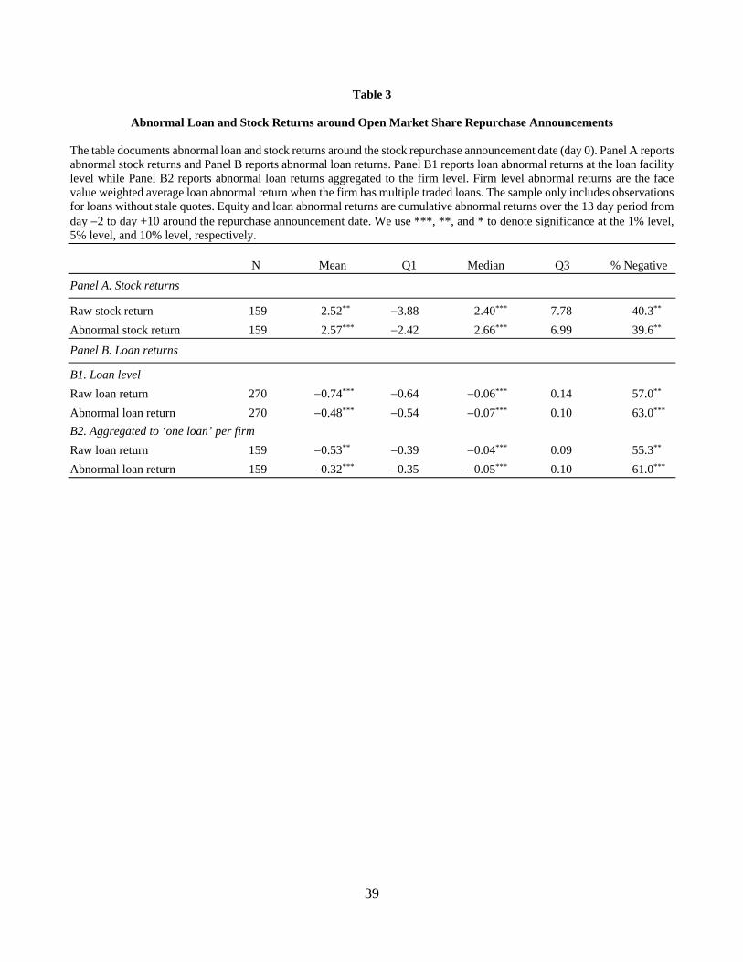
39

Table 3

Abnormal Loan and Stock Returns around Open Market Share Repurchase Announcements The table documents abnormal loan and stock returns around the stock repurchase announcement date (day 0). Panel A reports abnormal stock returns and Panel B reports abnormal loan returns. Panel B1 reports loan abnormal returns at the loan facility level while Panel B2 reports abnormal loan returns aggregated to the firm level. Firm level abnormal returns are the face value weighted average loan abnormal return when the firm has multiple traded loans. The sample only includes observations for loans without stale quotes. Equity and loan abnormal returns are cumulative abnormal returns over the 13 day period from day 2 to day +10 around the repurchase announcement date. We use ***, **, and * to denote significance at the 1% level, 5% level, and 10% level, respectively. N Mean Q1 Median Q3 % Negative

Panel A. Stock returns

Raw stock return 159 2.52** 3.88 2.40*** 7.78 40.3**

Abnormal stock return 159 2.57*** 2.42 2.66*** 6.99 39.6**

Panel B. Loan returns

B1. Loan level

Raw loan return 270 0.74*** 0.64 0.06*** 0.14 57.0**

Abnormal loan return 270 0.48*** 0.54 0.07*** 0.10 63.0***

B2. Aggregated to ‘one loan’ per firm

Raw loan return 159 0.53** 0.39 0.04*** 0.09 55.3**

Abnormal loan return 159 0.32*** 0.35 0.05*** 0.10 61.0***

40

Table 4

Correlations for the Repurchase Sample Spearman rank correlations between abnormal loan returns (Loan CAR), abnormal equity returns (Equity CAR), and firm and loan characteristics. We use ***, **, and * to denote significance at the 1% level, 5% level, and 10% level, respectively. 1 2 3 4 5 6 7 8 9 10 11 12 13 14 15 1 Loan CAR 1.000 2 Equity CAR 0.149** 1.000 3 Log equity value 0.100 0.085 1.000 4 Market leverage ratio 0.114 0.043 0.040 1.000 5 Leveraged recap. 0.141** 0.064 0.117* 0.269** 1.000 6 Tangibility 0.122* 0.195** 0.068 0.322** 0.061 1.000 7 Bank debt ratio 0.042 0.065 0.321* 0.136* 0.249*** 0.124* 1.000 8 Log bank relationship 0.122* 0.091 0.072 0.289** 0.316*** 0.159** 0.135* 1.000 9 Loan maturity 0.037 0.062 0.068 0.255** 0.256*** 0.050 0.200** 0.094 1.000 10 Institutional loan 0.040 0.043 0.053 0.009 0.147** 0.056 0.034 0.001 0.319* 1.000 11 Covenant intensity 0.100 0.024 0.598*** 0.320*** 0.284*** 0.091 0.145** 0.144** 0.009 0.083 1.000 12 Dividend restriction 0.150** 0.012 0.583* 0.237** 0.302*** 0.030 0.144** 0.102 0.124* 0.009 0.863** 1.000 13 Financial covenants 0.049 0.090 0.524* 0.334** 0.245*** 0.016 0.113 0.149** 0.149** 0.022 0.827** 0.800** 1.000 14 Incurrence covenants 0.141** 0.017 0.605*** 0.287*** 0.277*** 0.116* 0.171** 0.145** 0.017 0.089 0.981*** 0.871*** 0.736*** 1.000 15 TOM-Market 0.013 0.027 0.160** 0.088 0.474*** 0.003 0.202*** 0.021 0.111 0.034 0.192*** 0.247*** 0.170** 0.191*** 1.000

41

Table 5

Determinants of Loan Returns at Share Repurchase Announcements The table reports determinants of abnormal loan returns to open market share repurchase announcements. The dependent variable is the cumulative abnormal loan return (in decimal) from day 2 to day +10 around the share repurchase announcement date (day 0). Robust regressions employ a two-stage procedure to reduce the impact of outliers in the OLS regression. In the first step, the procedure drops influential outliers with a Cook’s D greater than 1. In the second step, an iterative procedure following Li (1985) reduces the weight of observations with large absolute residuals. Median (or quantile) regressions reduce the impact of outliers in the OLS regression by estimating the conditional median of the dependent variable. All variables are defined in Appendix A. T-statistics are based on robust standard errors and are clustered at the event/firm level. We use ***, **, and * to denote significance at the 1% level, 5% level, and 10% level, respectively.

Robust Median Robust Median Robust Median Robust Median OLS Regression Regression Regression Regression Regression Regression Regression Regression

(1) (2) (3) (4) (5) (6) (7) (8) (9)

Log market value 0.319 0.049 0.025 0.039 0.003 0.043 0.030 0.031 0.013 of equity (1.14) (1.58) (0.58) (1.33) (0.07) (1.38) (0.73) (0.95) (0.29)

Market leverage ratio 1.911* 0.626*** 0.936*** 0.604*** 0.857*** 0.775*** 0.845*** 0.692*** 0.821*** (1.93) (2.67) (3.30) (3.01) (3.20) (3.58) (3.08) (3.24) (2.77)

Leveraged recapitalization 0.666 0.569*** 0.491*** 0.602*** 0.538*** 0.523*** 0.412** 0.510*** 0.473*** (0.78) (3.82) (2.88) (4.52) (3.38) (3.41) (2.53) (2.93) (2.66)

Asset tangibility 2.341** 0.382* 0.548** 0.345** 0.520** 0.411** 0.546** 0.435** 0.637** (2.05) (1.97) (2.17) (2.01) (2.16) (2.19) (2.21) (2.15) (2.39)

Bank debt ratio 0.630 0.217* 0.242 0.178* 0.211 0.224* 0.298* 0.218* 0.334* (1.17) (1.91) (1.45) (1.68) (1.36) (1.97) (1.87) (1.88) (1.95)

Log length lead bank 0.223* 0.080** 0.129** 0.091** 0.148*** 0.099*** 0.121** 0.097** 0.120** relationship (1.71) (2.05) (2.38) (2.58) (2.93) (2.69) (2.33) (2.52) (2.13)

Loan maturity 0.194 0.009 0.015 0.017 0.015 0.008 0.009 0.002 0.011 (1.24) (0.69) (0.67) (1.41) (0.68) (0.60) (0.41) (0.16) (0.46)

Institutional loan 0.596** 0.017 0.063 0.051 0.147 0.046 0.080 0.022 0.076 (1.98) (0.27) (0.61) (0.89) (1.53) (0.71) (0.80) (0.35) (0.72)

TOM-Market 0.010 0.010*** 0.008* 0.010*** 0.007 0.004 0.007 0.004 0.006 (1.01) (4.37) (1.83) (4.86) (1.59) (1.29) (1.53) (1.30) (1.28)

Covenant intensity 0.108 0.049** 0.055* index (0.96) (2.39) (1.79) (continued)

42

Table 5 – continued

Robust Median Robust Median Robust Median Robust Median OLS Regression Regression Regression Regression Regression Regression Regression Regression

(1) (2) (3) (4) (5) (6) (7) (8) (9)

Incurrence covenant 0.138*** 0.167*** 0.400*** 0.261*** index (3.83) (-3.74) (5.40) (3.83)

Financial covenants 0.318*** 0.379** 0.068 0.034 0.031 0.083 dummy (2.78) (2.45) (0.40) (0.15) (0.17) (0.33)

Incurrence × Financial 0.317*** 0.176** covenants dummy (3.40) (2.00)

Dividend restriction 1.338*** 0.978*** dummy (4.71) (3.79)

Dividend × Financial 1.129*** 0.667* covenants dummy (3.30) (1.92)

Constant 3.948 0.160 0.015 0.051 0.253 0.395 0.166 0.274 0.005 (1.07) (0.42) (0.03) (0.15) (0.52) (0.98) (0.32) (0.67) (0.01)

Adj./Pseudo R2 0.13 0.21 0.04 0.28 0.06 0.39 0.07 0.34 0.06

Observations 270 268 270 268 270 268 270 268 270

43

Table 6

The Influence of the Relative Amount of Bank Debt to Total Debt on Loan Returns at Share Repurchase Announcements The table reports determinants of abnormal loan returns to open market share repurchase announcements. The dependent variable is the cumulative abnormal loan return (in decimal) from day 2 to day +10 around the share repurchase announcement date (day 0). Robust regressions employ a two-stage procedure to reduce the impact of outliers. In the first step, the procedure drops influential outliers with a Cook’s D greater than 1. In the second step, an iterative procedure following Li (1985) reduces the weight of observations with large absolute residuals. Median (or quantile) regressions reduce the impact of outliers by estimating the conditional median of the dependent variable. The bank debt ratio is the ratio of bank debt to total debt. The bank debt ratio quartile dummies are set equal to one when the bank debt ratio is in the lowest quartile (1st quartile dummy), second quartile (2nd quartile dummy), and third quartile (3rd quartile dummy), respectively. The left out or baseline group is the largest bank debt ratio quartile (4th quartile). The covenant and control variables are defined in Appendix A. T-statistics are based on robust standard errors and are clustered at the event/firm level. We use ***, **, and * to denote significance at the 1% level, 5% level, and 10% level, respectively.

Robust Median Robust Median Robust Median Robust Median Regression Regression Regression Regression Regression Regression Regression Regression

(1) (2) (3) (4) (5) (6) (7) (8)

Bank debt ratio 1st quartile dummy 0.241** 0.297* 0.226** 0.227** 0.262** 0.314** 0.254** 0.319* (2.18) (1.82) (2.12) (1.51) (2.37) (2.15) (2.26) (1.78)

Bank debt ratio 2nd quartile dummy 0.104 0.287* 0.071 0.167 0.101 0.233* 0.085 0.203 (1.19) (1.96) (0.81) (1.20) (1.15) (1.76) (0.96) (1.24)

Bank debt ratio 3rd quartile dummy 0.058 0.183 0.046 0.164 0.073 0.212 0.049 0.163 (0.63) (1.09) (0.52) (1.08) (0.80) (1.41) (0.56) (0.89)

Covenant intensity index 0.048** 0.074** (2.34) (2.17)

Incurrence covenant index 0.156*** 0.168*** 0.414*** 0.261*** (4.00) (3.52) (5.34) (3.82)

Financial covenants dummy 0.377*** 0.345** 0.082 0.114 0.067 0.019 (3.06) (2.03) (0.49) (0.51) (0.35) (0.06)

Incurrence × Financial 0.328*** 0.157* covenants dummy (3.40) (1.79)

Dividend restriction 1.358*** 0.946*** dummy (4.64) (3.20)

Dividend × Financial 1.122*** 0.750* Covenants dummy (3.19) (1.88)

Constant 0.027 0.135 0.171 0.391 0.201 0.199 0.063 0.342 (0.07) (0.24) (0.47) (0.73) (0.51) (0.37) (0.16) (0.52)

Controls Yes Yes Yes Yes Yes Yes Yes Yes

Adj./Pseudo R2 0.22 0.04 0.28 0.06 0.39 0.07 0.34 0.06

Observations 268 270 268 270 268 270 268 270

44

Table 7

Relation between Changes in Stock Value and Loan Value at Stock Repurchase Announcement

The table reports robust and median regressions of abnormal stock dollar returns on abnormal loan dollar returns. Robust regressions employ a two-stage procedure to reduce the impact of outliers. In the first step, the procedure drops influential outliers with a Cook’s D greater than 1. In the second step, an iterative procedure following Li (1985) reduces the weight of observations with large absolute residuals. Median (or quantile) regressions reduce the impact of outliers by estimating the conditional median of the dependent variable. The abnormal stock dollar return is computed as the cumulative abnormal equity return over days 2 to +10 relative to the stock repurchase announcement (day 0) multiplied by the market value of equity on day 3. The abnormal loan dollar return is computed as the cumulative abnormal loan return over days 2 to +10 relative to the stock repurchase announcement (day 0) multiplied by the sum of long-term debt and debt in current liabilities at the fiscal year-end immediately prior to the stock repurchase announcement. T-statistics are based on robust standard errors which are clustered at the event/firm level. We use ***, **, and * to denote significance at the 1% level, 5% level, and 10% level, respectively.

Dependent variable: Abnormal stock dollar return ————————————————————————— Loan level Firm level ——————————— ——————————— Robust Median Robust Median Regression Regression Regression Regression

Independent variables (1) (2) (3) (4)

Abnormal loan dollar return 0.711 0.745 2.528 2.377 (15.19)*** (10.34)*** (11.79)*** (8.33)***

Log market value of equity 25.434 25.734 17.027 25.512 (1.71)* (0.93) (1.98)* (1.75)

Constant 157.216 133.200 89.296 133.853 (1.55) (0.74) (1.51) (1.17)

Adj./Pseudo R2 0.37 0.02 0.56 0.05

Observations 268 270 157 159

45

Table 8

The Influence of Bank Debt on the Relation between Changes in Stock Value and Loan Value at Stock Repurchase Announcement

The table reports robust and median regressions of abnormal stock dollar returns on abnormal loan dollar returns conditioned on quartiles of the ratio of bank debt to total debt. Panel A reports the regressions while Panel B summarizes the coefficients on abnormal loan dollar return by bank debt ratio quartile. Robust regressions employ a two-stage procedure to reduce the impact of outliers. In the first step, the procedure drops influential outliers with a Cook’s D greater than 1. In the second step, an iterative procedure following Li (1985) reduces the weight of observations with large absolute residuals. Median (or quantile) regressions reduce the impact of outliers by estimating the conditional median of the dependent variable. The abnormal stock dollar return is computed as the cumulative abnormal equity return over days 2 to +10 relative to the stock repurchase announcement (day 0) multiplied by the market value of equity on day 3. The abnormal loan dollar return is computed as the cumulative abnormal loan return over days 2 to +10 relative to the stock repurchase announcement (day 0) multiplied by the sum of long-term debt and debt in current liabilities at the fiscal year-end immediately prior to the stock repurchase announcement. The bank debt ratio is the ratio of bank debt to total debt. The bank debt ratio quartile dummies are set equal to one when the bank debt ratio is in the lowest quartile (1st quartile dummy), second quartile (2nd quartile dummy), and third quartile (3rd quartile dummy), respectively. The left out or baseline group is the largest bank debt ratio quartile (4th quartile). T-statistics are based on robust standard errors which are clustered at the event/firm level. We use ***, **, and * to denote significance at the 1% level, 5% level, and 10% level, respectively.



Panel A. Regressions conditioning abnormal loan dollar return by bank debt ratio quartile

Abnormal loan dollar return 0.016 1.030*** 2.491*** 1.676** (0.06) (2.77) (4.83) (2.58)

Abnormal loan dollar return × 0.674** 0.310 2.859*** 1.992* Bank debt ratio 1st quartile dummy (2.56) (0.78) (5.44) (1.80)

Abnormal loan dollar return × 1.192* 0.979 0.662 0.720 Bank debt ratio 2nd quartile dummy (1.79) (0.88) (1.09) (0.64)

Abnormal loan dollar return × 2.492*** 1.669** 0.247 1.032 Bank debt ratio 3rd quartile dummy (6.02) (2.15) (0.44) (1.23)

Bank debt ratio 1st quartile dummy 37.056 48.912 19.350 57.225 (0.80) (0.66) (0.60) (0.83)

Bank debt ratio 2nd quartile dummy 71.299 1.412 84.421** 19.916 (1.52) (0.02) (2.56) (0.31)

Bank debt ratio 3rd quartile dummy 55.591 103.685 9.322 99.159 (1.29) (1.46) (0.27) (1.52)

Log market value of equity 7.384 16.210 19.951* 13.981 (0.43) (0.83) (1.91) (0.82)

Constant 26.315 39.913 128.095 11.189 (0.21) (0.23) (1.57) (0.08)

Adj./Pseudo R2 0.45 0.06 0.58 0.06

Observations 268 270 157 159 (continued)

46

Table 8 – continued


Bank debt ratio quartiles (1) (2) (3) (4)

Panel B. Coefficients on abnormal loan dollar return by bank debt ratio quartile

Lowest : Bank debt ratio 1st quartile 0.658** 0.720** 0.368 0.316 Bank debt ratio 2nd quartile 1.176*** 2.009*** 1.829*** 2.396*** Bank debt ratio 3rd quartile 2.476*** 2.699*** 2.738*** 2.708*** Highest: Bank debt ratio 4th quartile 0.016 1.030*** 2.491*** 1.676**

47

Table 9

Abnormal Loan and Stock Returns around SEO Announcements The table documents abnormal loan and stock returns around the seasoned equity offering (SEO) announcement day (day 0). Panel A reports abnormal stock returns and Panel B reports abnormal loan returns. Panel B1 reports loan abnormal returns at the loan facility level while Panel B2 reports abnormal loan returns aggregated to the firm level. Firm level abnormal returns are the face value weighted average loan abnormal return when the firm has multiple traded loans. The sample only includes observations for loans without stale quotes. Equity and loan abnormal returns are cumulative abnormal returns over the 13 day period from day 2 to day +10 around the repurchase announcement date. We use ***, **, and * to denote significance at the 1% level, 5% level, and 10% level, respectively. N Mean Q1 Median Q3 % Negative

Panel A. Stock returns

Raw stock return 104 0.78*** 7.04 0.63*** 5.49 51.9

Abnormal stock return 104 1.22*** 8.39 1.38*** 4.27 57.6**

Panel B. Loan returns

B1. Loan level

Raw loan return 167 0.61** 0.08 0.09*** 0.84 35.3***

Abnormal loan return 167 0.50** 0.16 0.01** 0.58 47.9

B2. Aggregated to ‘one loan’ per firm

Raw loan return 104 0.51* 0.07 0.08*** 0.61 34.6***

Abnormal loan return 104 0.41* 0.16 0.00 0.51 50.0

48

Table 10

Relation between Changes in Stock Value and Loan Value at SEO Announcement

The table reports robust and median regressions of abnormal stock dollar returns on abnormal loan dollar returns. Robust regressions employ a two-stage procedure to reduce the impact of outliers. In the first step, the procedure drops influential outliers with a Cook’s D greater than 1. In the second step, an iterative procedure following Li (1985) reduces the weight of observations with large absolute residuals. Median (or quantile) regressions reduce the impact of outliers by estimating the conditional median of the dependent variable. The abnormal stock dollar return is computed as the cumulative abnormal equity return over days 2 to +10 relative to the seasoned equity offering (SEO) announcement (day 0) multiplied by the market value of equity on day 3. The abnormal loan dollar return is computed as the cumulative abnormal loan return over days 2 to +10 relative to the seasoned equity offering (SEO) announcement (day 0) multiplied by the sum of long-term debt and debt in current liabilities at the fiscal year-end immediately prior to the stock repurchase announcement. T-statistics are based on robust standard errors and are clustered at the event/firm level. We use ***, **, and * to denote significance at the 1% level, 5% level, and 10% level, respectively.



Abnormal loan dollar return 0.281 0.279 0.250 0.247 (126.7)*** (33.33)*** (90.71)*** (14.29)***

Log market value of equity 38.767 24.663 32.848 42.999 (3.61)*** (1.46) (2.86)*** (1.90)*

Constant 242.134 131.232 205.572 261.922 (3.29)*** (0.99) (2.66)*** (1.50)

Adj./Pseudo R2 0.94 0.23 0.91 0.15

Observations 164 167 101 104

49

Figure 1. Trading volume ($ billions)of syndicated loans. Source: Thomson Reuters LPC.

$0

$100

$200

$300

$400

$500

$600

1991 1992 1993 1994 1995 1996 1997 1998 1999 2000 2001 2002 2003 2004 2005 2006 2007 2008 2009 2010 2011 2012 2013

50

Figure 2. Loan and stock price performance around stock repurchase announcements. This figure shows cumulative abnormal loan and equity returns in event time around stock repurchase announcements. Loan and stock cumulative abnormal returns are computed at the firm level. Multiple loan returns are aggregated to the firm level using the market value weighted average of multiple issues. ECAR denotes stock cumulative abnormal returns, LCR denotes cumulative raw loan returns, and LCAR denotes cumulative abnormal loan returns. Section 2 discusses how we compute abnormal loan and equity returns.

51

Figure 3. Loan and stock price performance around seasoned equity offering announcements. This figure shows cumulative abnormal loan and equity returns in event time around seasoned equity offering announcements. Loan and stock cumulative abnormal returns are computed at the firm level. Multiple loan returns are aggregated to the firm level using the market value weighted average of multiple issues. ECAR denotes stock cumulative abnormal returns, LCR denotes cumulative raw loan returns, and LCAR denotes cumulative abnormal loan returns. Section 2 discusses how we compute abnormal loan and equity returns.

Bank Loan Price Reactions to Corporate Events: Evidence ... Loan Price Reactions to... · Bank Loan...

Documents

Transcript of Bank Loan Price Reactions to Corporate Events: Evidence ... Loan Price Reactions to... · Bank Loan...