Bandstructure Calculations in FDTD Solutions · Find photonic band gaps (frequency ranges where...

Bandstructure Calculations in FDTD Solutions

LUMERICAL SOLUTIONS INC.

PROPRIETARY AND CONFIDENTIAL© LUMERICAL SOLUTIONS INC

1

OutlineIntroduction

Simulation methodologySimulation setupAnalysis

Demonstration (2D triangular lattice)

Simulations with lossProblems associated with lossTipsExample (1D chain of metallic spheres)

Q&A


2

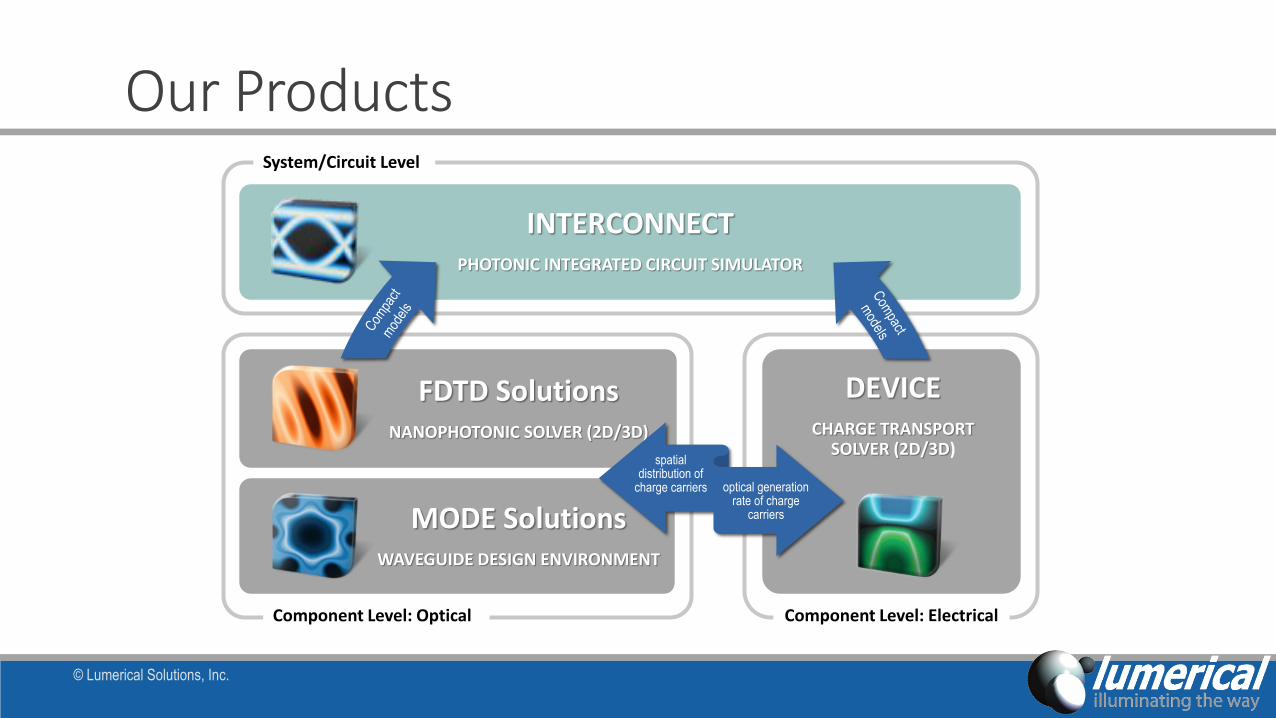
Our Products

© Lumerical Solutions, Inc.

FDTD SolutionsNANOPHOTONIC SOLVER (2D/3D)

MODE SolutionsWAVEGUIDE DESIGN ENVIRONMENT

spatial distribution of

charge carriers optical generation rate of charge

carriers

INTERCONNECTPHOTONIC INTEGRATED CIRCUIT SIMULATOR

DEVICECHARGE TRANSPORT

SOLVER (2D/3D)

System/Circuit Level

Component Level: Optical Component Level: Electrical

Lumerical SolutionsLumerical empowers R&D professionals with best-in-class design tools and services to support the creation of better photonic technologies

© Lumerical Solutions, Inc.

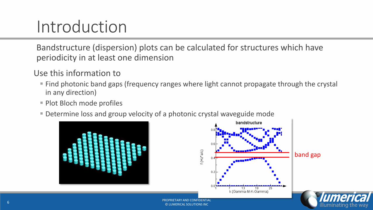
IntroductionBandstructure (dispersion) plots can be calculated for structures which have periodicity in at least one dimension

Use this information to Find photonic band gaps (frequency ranges where light cannot propagate through the crystal

in any direction)

Plot Bloch mode profiles

Determine loss and group velocity of a photonic crystal waveguide mode


6

band gap

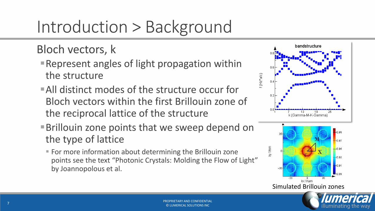
Introduction > BackgroundBloch vectors, kRepresent angles of light propagation within

the structure

All distinct modes of the structure occur for Bloch vectors within the first Brillouin zone of the reciprocal lattice of the structure

Brillouin zone points that we sweep depend on the type of lattice For more information about determining the Brillouin zone

points see the text “Photonic Crystals: Molding the Flow of Light” by Joannopolous et al.


7

Simulated Brillouin zones

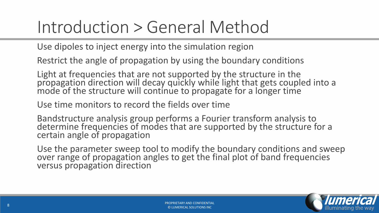
Introduction > General MethodUse dipoles to inject energy into the simulation region

Restrict the angle of propagation by using the boundary conditions

Light at frequencies that are not supported by the structure in the propagation direction will decay quickly while light that gets coupled into a mode of the structure will continue to propagate for a longer time

Use time monitors to record the fields over time

Bandstructure analysis group performs a Fourier transform analysis to determine frequencies of modes that are supported by the structure for a certain angle of propagation

Use the parameter sweep tool to modify the boundary conditions and sweep over range of propagation angles to get the final plot of band frequencies versus propagation direction


8

Introduction > FDTDFinite Difference Time Domain (FDTD) is a state-of-the-art method for solving Maxwell’s equations for complex geometriesFew inherent approximations

General technique that can deal with many types of problems

Arbitrary complex geometries

One simulation gives broadband results

Not just for bandstructure calculation, but can also simulate other devices such as waveguides, photonic crystal cavities, etc.


10

Simulation Methodology > OverviewSimulation setupParameterizationStructureSimulation regionSources and monitors

CalculationsFourier transformSummation of FFTsSweep over kCollecting results


11

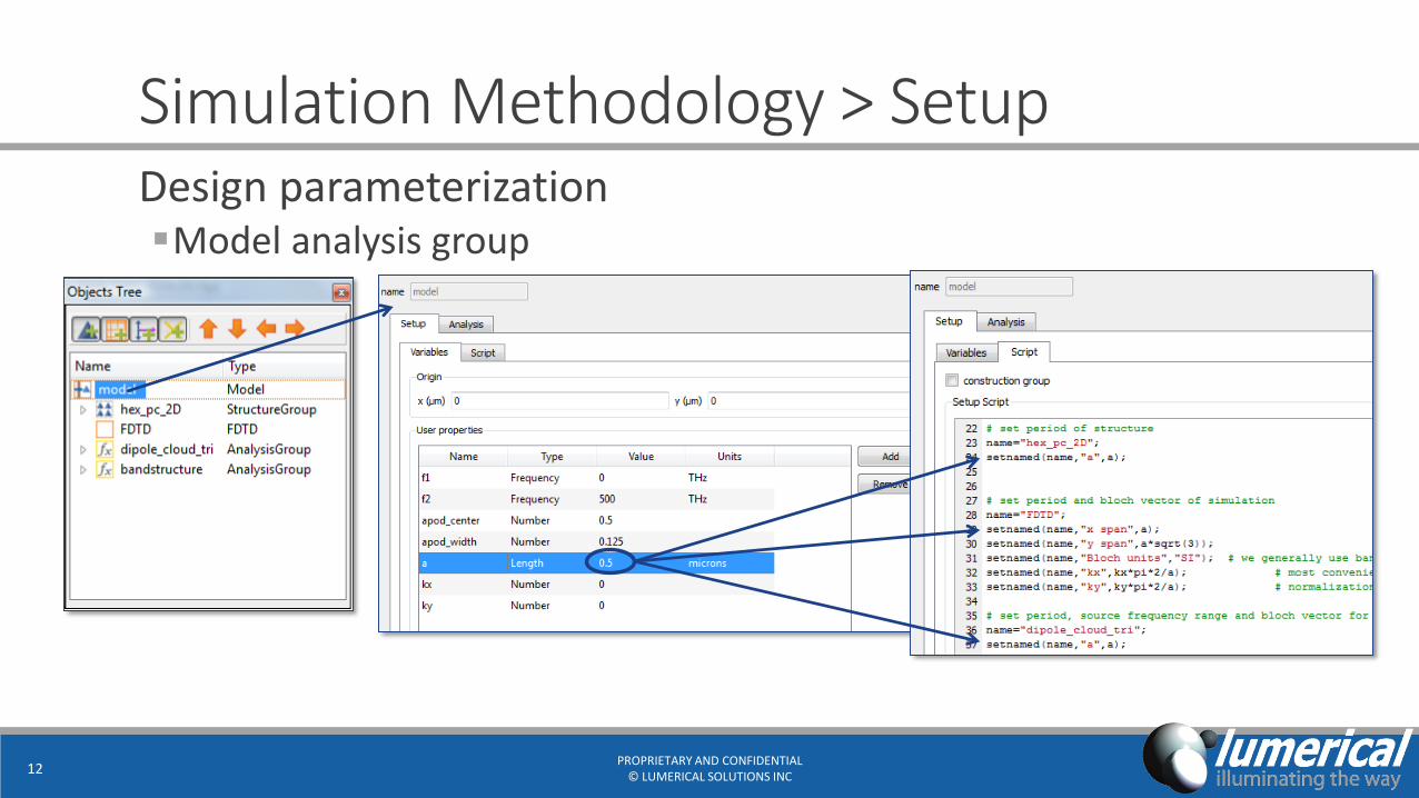
Simulation Methodology > SetupDesign parameterizationModel analysis group


12

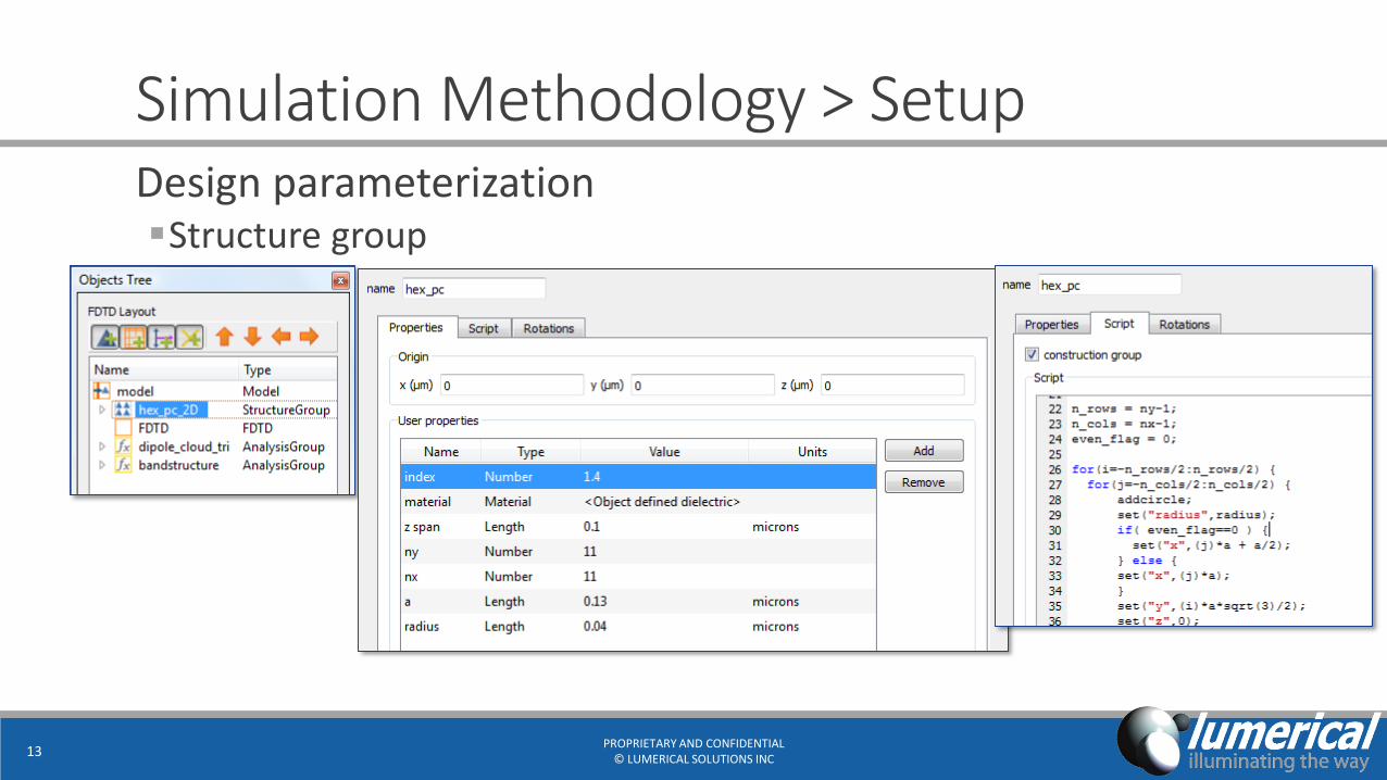
Simulation Methodology > Setup


13

Design parameterizationStructure group

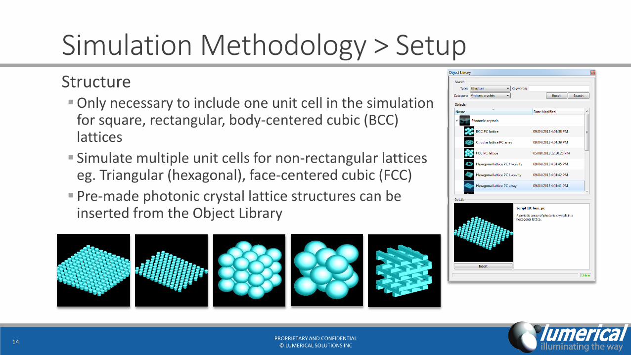
Simulation Methodology > SetupStructureOnly necessary to include one unit cell in the simulation

for square, rectangular, body-centered cubic (BCC) lattices

Simulate multiple unit cells for non-rectangular lattices eg. Triangular (hexagonal), face-centered cubic (FCC)

Pre-made photonic crystal lattice structures can be inserted from the Object Library


14

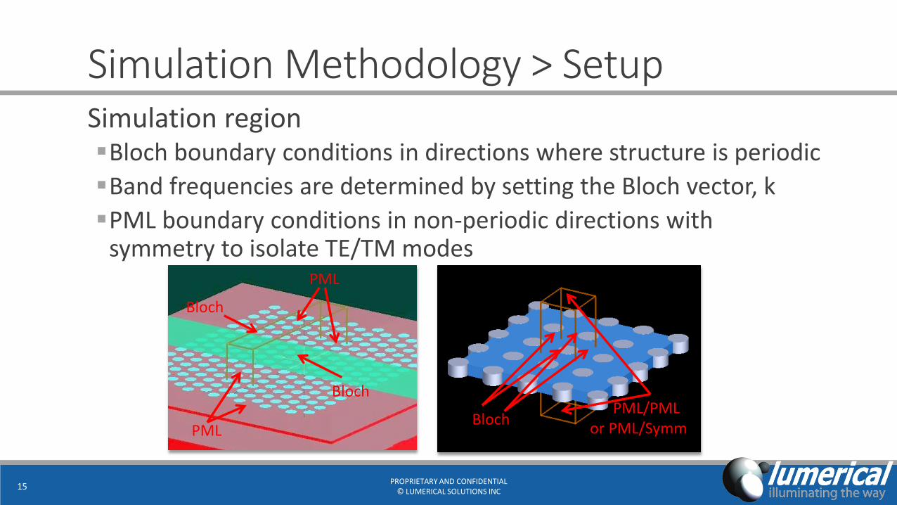
Simulation Methodology > SetupSimulation regionBloch boundary conditions in directions where structure is periodic

Band frequencies are determined by setting the Bloch vector, k

PML boundary conditions in non-periodic directions with symmetry to isolate TE/TM modes


15

BlochPML/PML

or PML/Symm

Bloch

Bloch

PML

PML

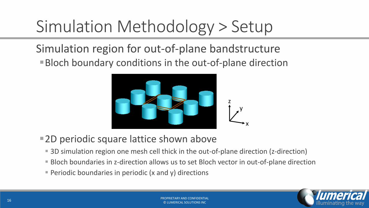
Simulation Methodology > SetupSimulation region for out-of-plane bandstructureBloch boundary conditions in the out-of-plane direction


16

2D periodic square lattice shown above 3D simulation region one mesh cell thick in the out-of-plane direction (z-direction)

Bloch boundaries in z-direction allows us to set Bloch vector in out-of-plane direction

Periodic boundaries in periodic (x and y) directions

x

yz

Simulation Methodology > SetupSimulation region for non-rectangular latticesFDTD simulation region is rectangular so for non-rectangular

lattices, multiple unit cells can be included in the simulation to form a rectangular unit cell

If multiple unit cells of the structure are included in the simulation region, mesh step size needs to be adjusted to include an integer number of mesh cells in each unit cell Ensures that each unit cell is meshed the same way


17

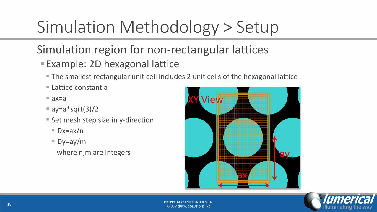
Simulation Methodology > SetupSimulation region for non-rectangular latticesExample: 2D hexagonal lattice The smallest rectangular unit cell includes 2 unit cells of the hexagonal lattice

Lattice constant a

ax=a

ay=a*sqrt(3)/2

Set mesh step size in y-direction

Dx=ax/n

Dy=ay/m

where n,m are integers


18

XY View

ax

ay

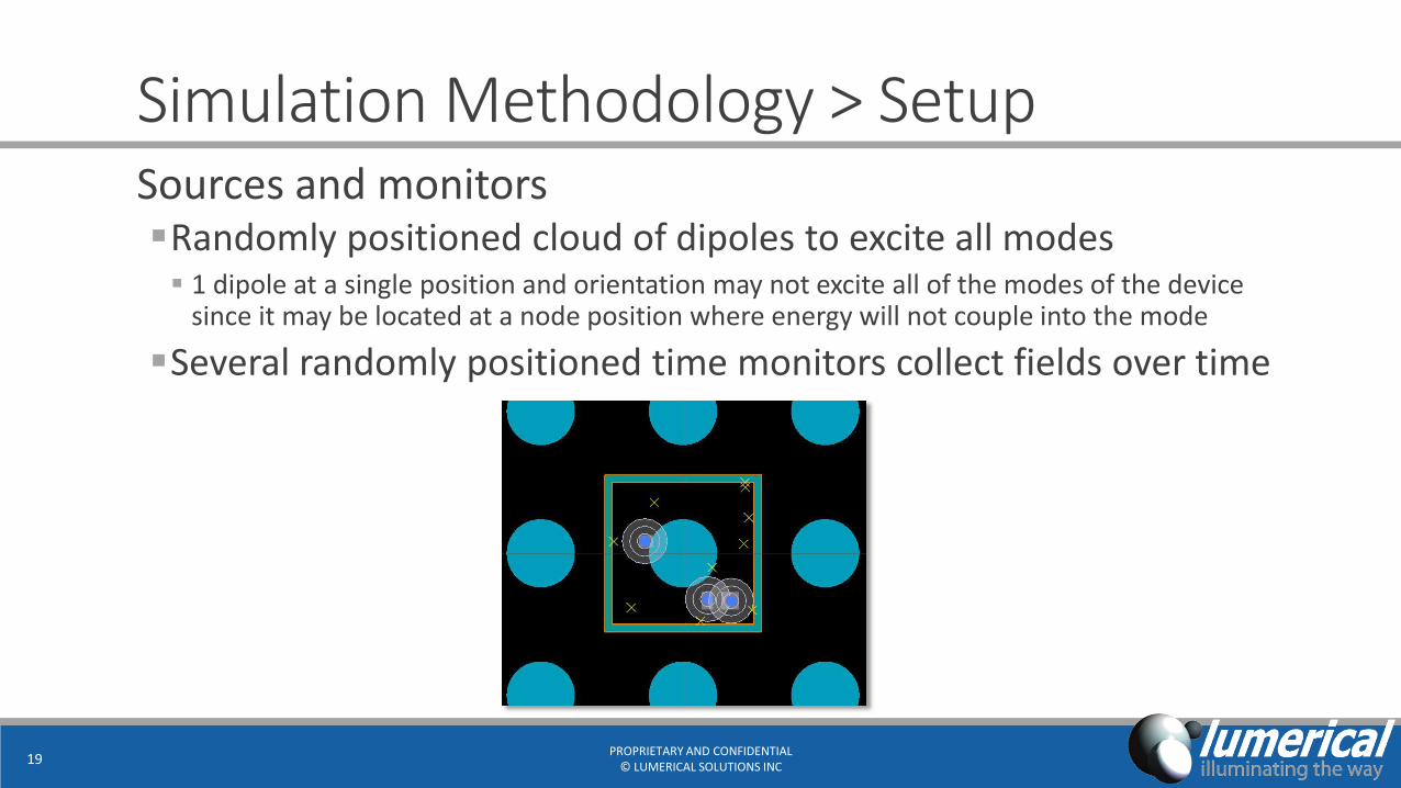
Simulation Methodology > SetupSources and monitorsRandomly positioned cloud of dipoles to excite all modes 1 dipole at a single position and orientation may not excite all of the modes of the device

since it may be located at a node position where energy will not couple into the mode

Several randomly positioned time monitors collect fields over time


19

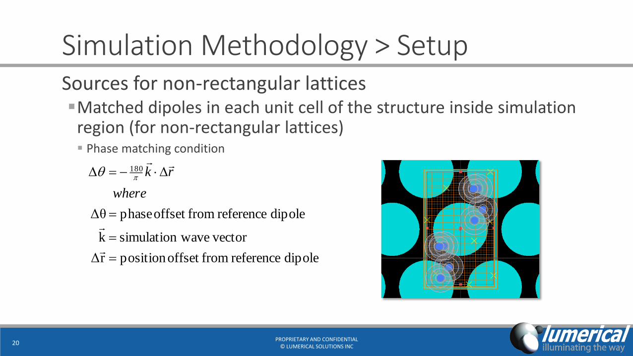
Simulation Methodology > SetupSources for non-rectangular latticesMatched dipoles in each unit cell of the structure inside simulation

region (for non-rectangular lattices) Phase matching condition


20

dipole reference fromoffset position rΔ

vector wavesimulationk

dipole reference fromoffset phaseΔθ

180

where

rk

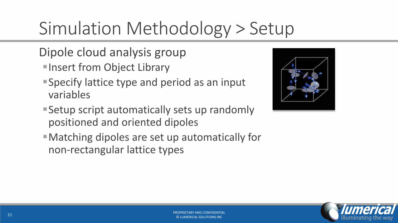
Simulation Methodology > SetupDipole cloud analysis groupInsert from Object Library

Specify lattice type and period as an input variables

Setup script automatically sets up randomly positioned and oriented dipoles

Matching dipoles are set up automatically for non-rectangular lattice types


21

Simulation Methodology > SetupSummary of setup methodParameterize using Model analysis group and structure groups

Use Bloch boundaries in periodic directions

Random cloud of dipoles and monitors

Rectangular lattices Only need to include 1 unit cell in the simulation region

Non-rectangular lattices Include multiple unit cells that form the smallest rectangular unit cell

Each unit cell should be meshed the same way

Matching dipole positions in each unit cell with phase matching


22

Simulation Methodology > CalculationsOverview of calculation:

Step 1 – Fourier transform to get spectrum

Step 2 – Summation of spectra

Step 3 – Repeat for all k

Step 4 – Collect sweep results, find resonances


23

Simulation Methodology > CalculationsFourier transformApply apodization to filter out start and end effects Applies Gaussian windowing function to the time domain fields to exclude transient fields Apodization parameters are set in the bandstructure analysis group

Apply Fast Fourier transform (FFT) to apodized time signal to get the spectrum


24

Simulation Methodology > CalculationsSummation of spectraSum the Fourier transformed time signals from each field

component of each time monitor

Summing over several monitors ensures that all resonant frequencies are found even if one monitors is located in a node of a particular mode

Fourier transform and summation are done using the banstructure analysis group which can be inserted from the Object Library


25

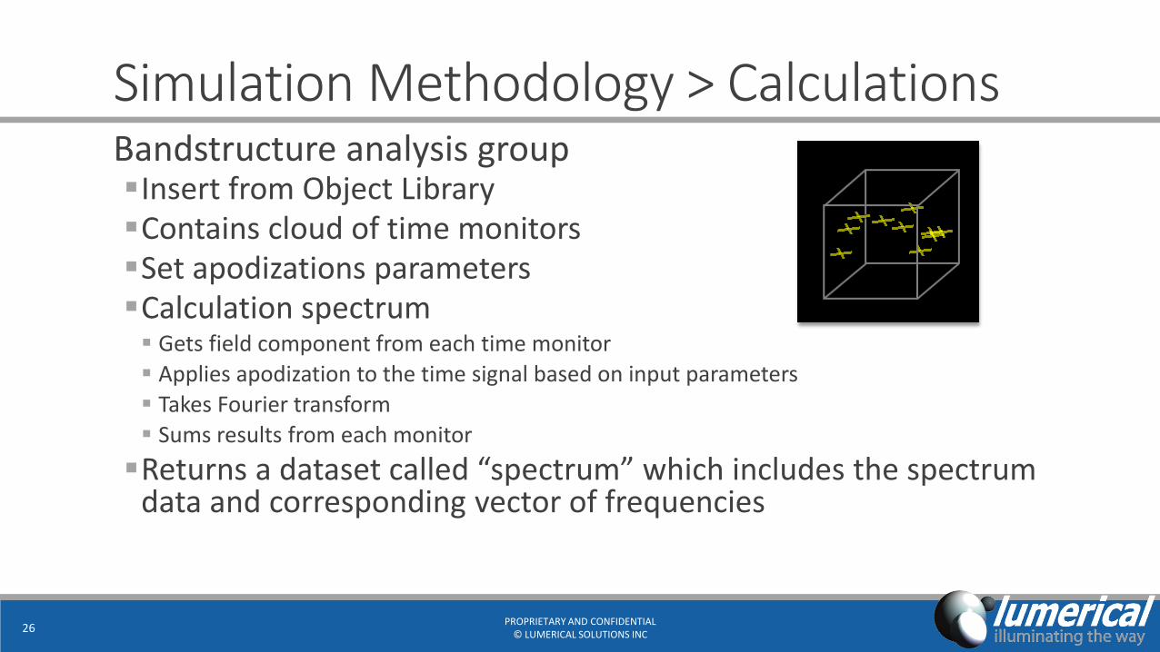
Simulation Methodology > CalculationsBandstructure analysis groupInsert from Object LibraryContains cloud of time monitorsSet apodizations parametersCalculation spectrum Gets field component from each time monitor

Applies apodization to the time signal based on input parameters

Takes Fourier transform

Sums results from each monitor

Returns a dataset called “spectrum” which includes the spectrum data and corresponding vector of frequencies


26

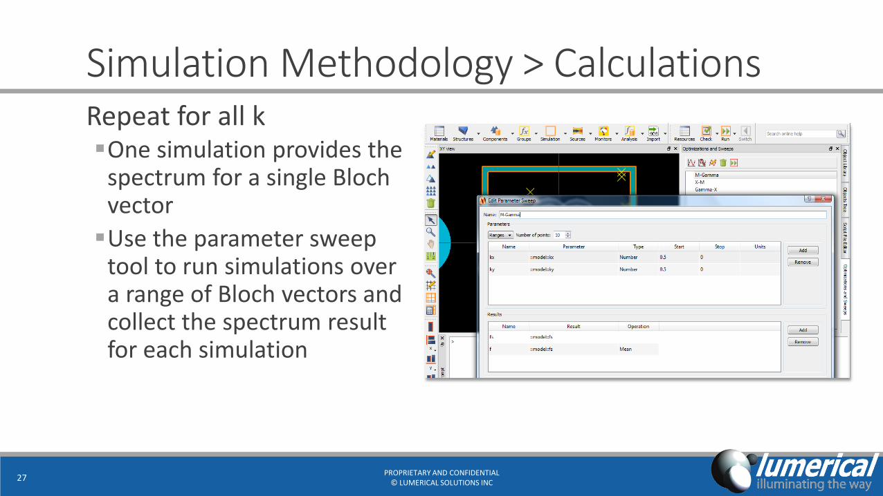
Simulation Methodology > CalculationsRepeat for all kOne simulation provides the

spectrum for a single Bloch vector

Use the parameter sweep tool to run simulations over a range of Bloch vectors and collect the spectrum result for each simulation


27

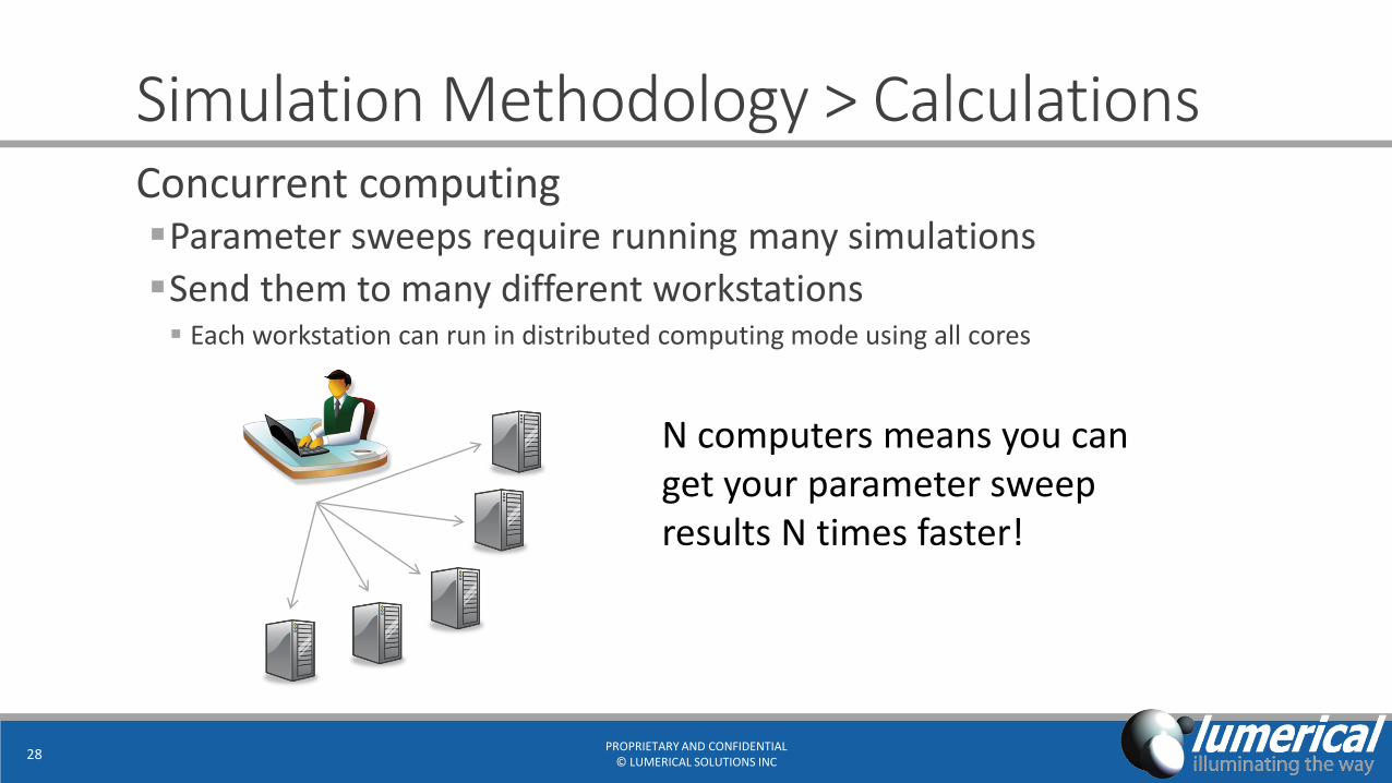
Simulation Methodology > CalculationsConcurrent computingParameter sweeps require running many simulations

Send them to many different workstations Each workstation can run in distributed computing mode using all cores


28

N computers means you can get your parameter sweep results N times faster!

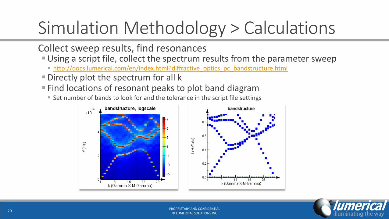
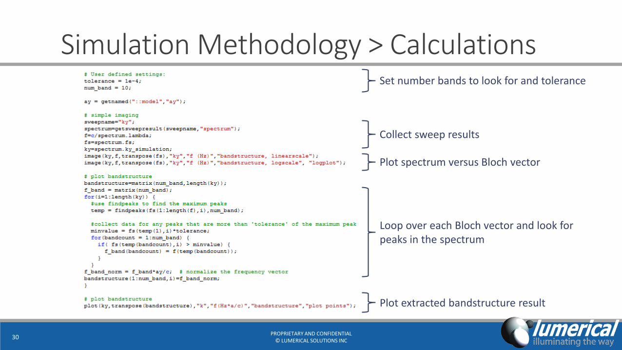
Simulation Methodology > CalculationsCollect sweep results, find resonancesUsing a script file, collect the spectrum results from the parameter sweep http://docs.lumerical.com/en/index.html?diffractive_optics_pc_bandstructure.html

Directly plot the spectrum for all k Find locations of resonant peaks to plot band diagram Set number of bands to look for and the tolerance in the script file settings


29

http://docs.lumerical.com/en/index.html?diffractive_optics_pc_bandstructure.html

Simulation Methodology > Calculations


30

Set number bands to look for and tolerance

Collect sweep results

Plot spectrum versus Bloch vector

Plot extracted bandstructure result

Loop over each Bloch vector and look for peaks in the spectrum

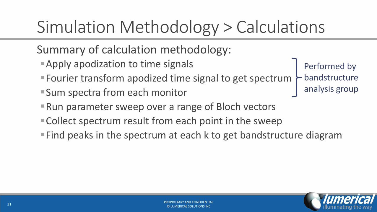
Simulation Methodology > CalculationsSummary of calculation methodology:Apply apodization to time signals

Fourier transform apodized time signal to get spectrum

Sum spectra from each monitor

Run parameter sweep over a range of Bloch vectors

Collect spectrum result from each point in the sweep

Find peaks in the spectrum at each k to get bandstructure diagram


31

Performed by bandstructureanalysis group

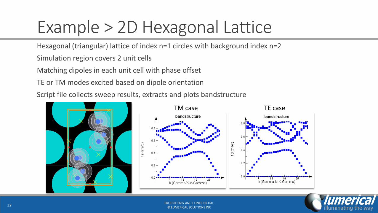
Example > 2D Hexagonal LatticeHexagonal (triangular) lattice of index n=1 circles with background index n=2

Simulation region covers 2 unit cells

Matching dipoles in each unit cell with phase offset

TE or TM modes excited based on dipole orientation

Script file collects sweep results, extracts and plots bandstructure


32

TM case TE case

Simulations With LossProblems associated with loss

Tips for lossy simulationsSource and monitor placement

Apodization settings

Symmetry boundary conditions

Source spectrum

Tolerance

Particle chain example


33

Simulations With Loss > Problems AssociatedSources of lossAbsorbing materialsRadiation

Problems associated with lossResonant fields decay quickly Useful part of the time signal is shortened

Fourier transform of time signal is noisy Difficult to extract resonant peaks

With more deliberate setup, we can increase the strength of the signal from modes that we are interested in and decrease the signal from other modes and noise so we can more easily extract a clear bandstructure diagram


34

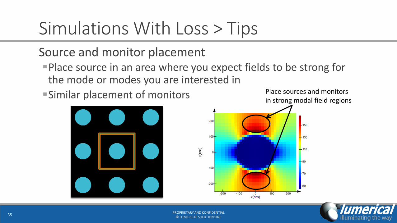
Simulations With Loss > TipsSource and monitor placementPlace source in an area where you expect fields to be strong for

the mode or modes you are interested in

Similar placement of monitors


35

Place sources and monitorsin strong modal field regions

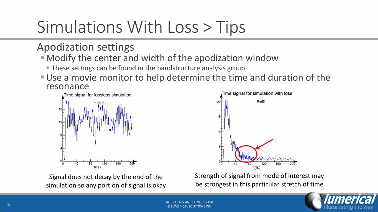
Simulations With Loss > TipsApodization settingsModify the center and width of the apodization window These settings can be found in the bandstructure analysis group

Use a movie monitor to help determine the time and duration of the resonance


36

Strength of signal from mode of interest may be strongest in this particular stretch of time

Signal does not decay by the end of the simulation so any portion of signal is okay

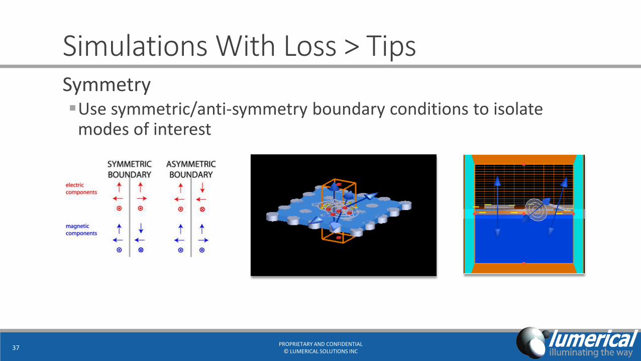
Simulations With Loss > TipsSymmetryUse symmetric/anti-symmetry boundary conditions to isolate

modes of interest


37

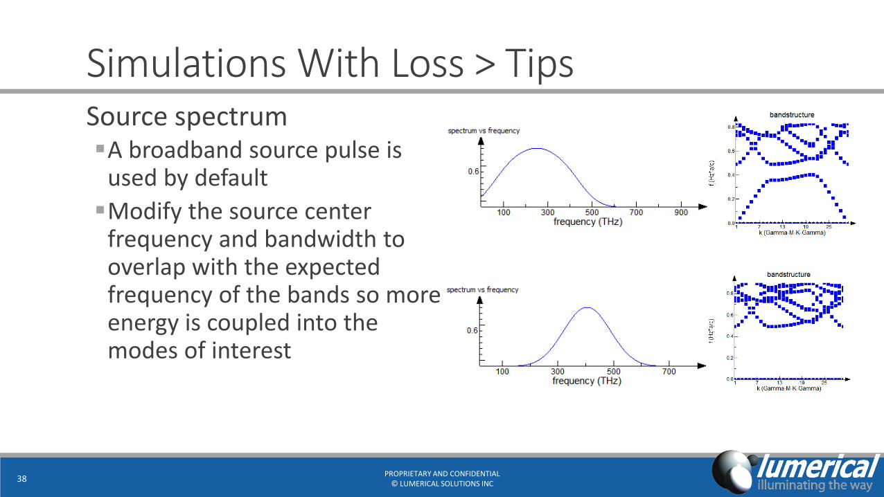
Simulations With Loss > TipsSource spectrumA broadband source pulse is

used by default

Modify the source center frequency and bandwidth to overlap with the expected frequency of the bands so more energy is coupled into the modes of interest


38

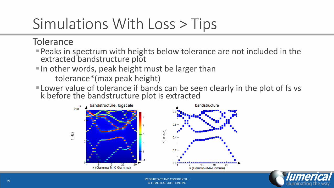
Simulations With Loss > TipsTolerancePeaks in spectrum with heights below tolerance are not included in the

extracted bandstructure plot In other words, peak height must be larger than

tolerance*(max peak height)Lower value of tolerance if bands can be seen clearly in the plot of fs vs

k before the bandstructure plot is extracted


39

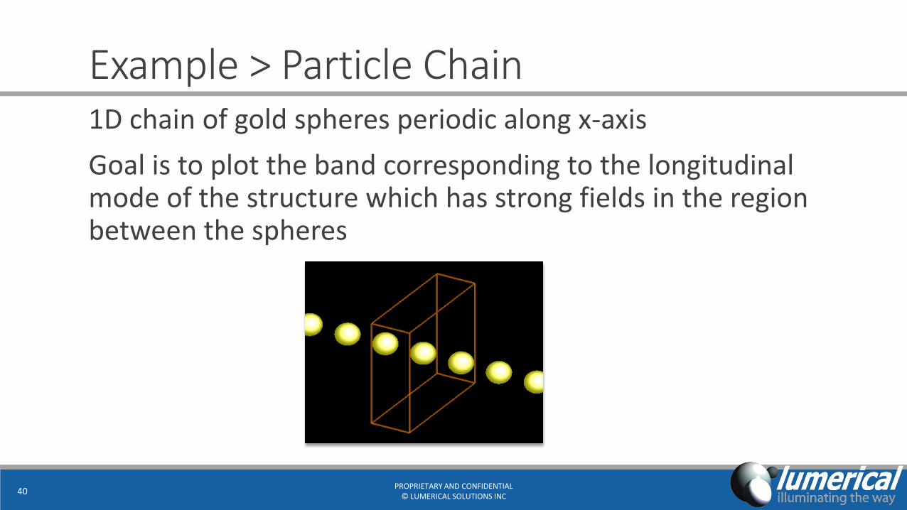
Example > Particle Chain1D chain of gold spheres periodic along x-axis

Goal is to plot the band corresponding to the longitudinal mode of the structure which has strong fields in the region between the spheres


40

Example > Particle ChainWith the typical method of using random cloud of dipoles we are not able to clearly extract the band of interestTransverse modes of the chain are also excited

Not enough energy is coupled into the longitudinal mode to extract a clear resonance peak


41

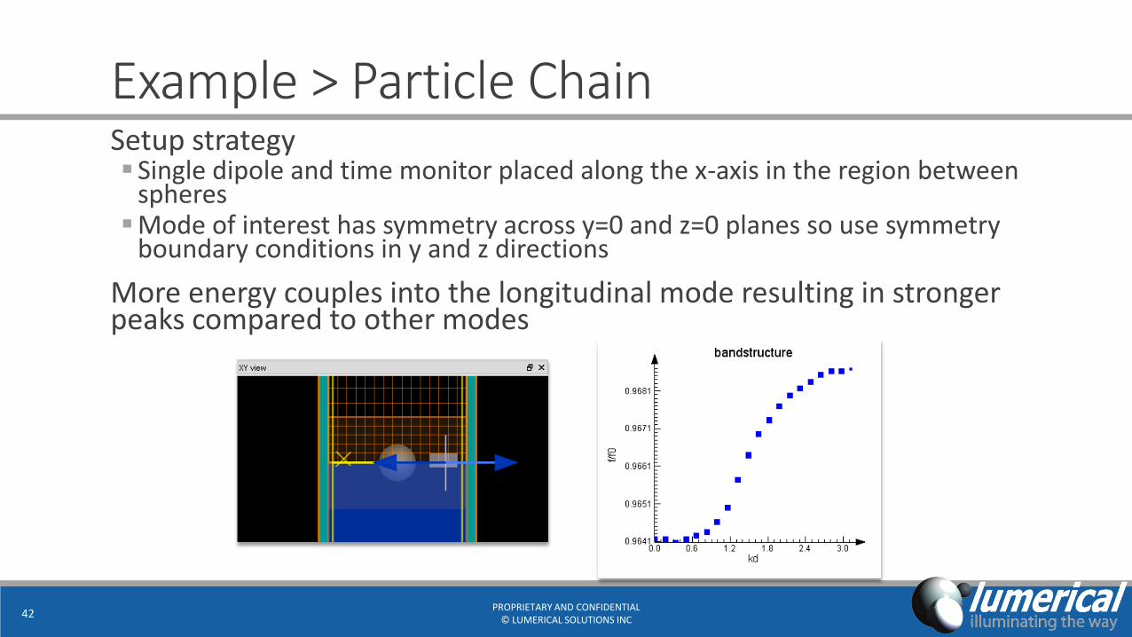
Example > Particle ChainSetup strategy Single dipole and time monitor placed along the x-axis in the region between

spheresMode of interest has symmetry across y=0 and z=0 planes so use symmetry

boundary conditions in y and z directions

More energy couples into the longitudinal mode resulting in stronger peaks compared to other modes


42

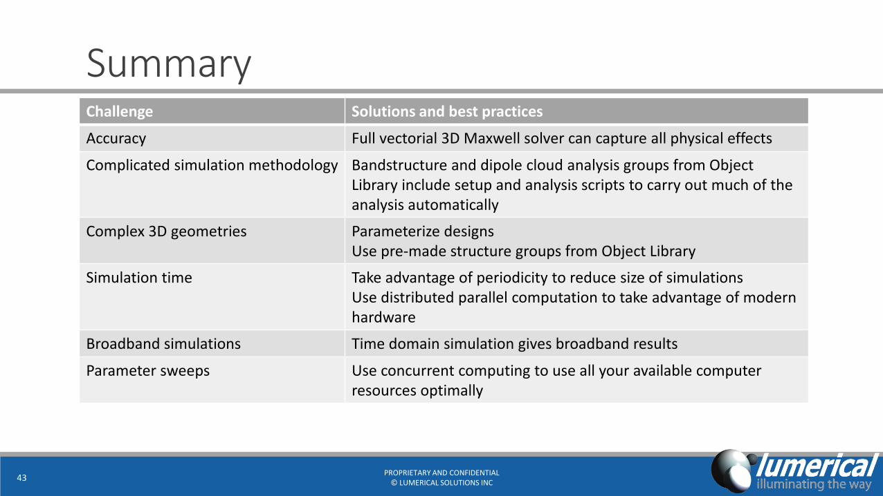
SummaryChallenge Solutions and best practices

Accuracy Full vectorial 3D Maxwell solver can capture all physical effects

Complicated simulation methodology Bandstructure and dipole cloud analysis groups from Object Library include setup and analysis scripts to carry out much of the analysis automatically

Complex 3D geometries Parameterize designsUse pre-made structure groups from Object Library

Simulation time Take advantage of periodicity to reduce size of simulationsUse distributed parallel computation to take advantage of modern hardware

Broadband simulations Time domain simulation gives broadband results

Parameter sweeps Use concurrent computing to use all your available computer resources optimally


43

Questions? [email protected]

Sales Inquiries: [email protected]

Contact your local Lumerical representative

Start your free 30 day trial today www.lumerical.com

Contact Us

Connect with Lumerical

www.lumerical.com


44

mailto:[email protected]

mailto:[email protected]

https://www.lumerical.com/company/representatives.html

https://www.lumerical.com/downloads

https://www.linkedin.com/company/lumerical-solutions-inc

https://www.linkedin.com/company/lumerical-solutions-inc

https://www.youtube.com/user/Lumerical

https://www.youtube.com/user/Lumerical

https://twitter.com/Lumerical

https://twitter.com/Lumerical

https://plus.google.com/103293326702121890306

https://plus.google.com/103293326702121890306

Bandstructure Calculations in FDTD Solutions · Find photonic band gaps (frequency ranges where...

Documents

Transcript of Bandstructure Calculations in FDTD Solutions · Find photonic band gaps (frequency ranges where...