Balancing of Network Energy using Observer Approach · Balancing of Network Energy using Observer...
90
Balancing of Network Energy using Observer Approach Master Thesis Submitted in Fulfilment of the Requirements for the Academic Degree M.Sc. Dept. of Computer Science Chair of Computer Engineering Submitted by: Sai Ram Charan Patharlapati Student ID: 358730 Date: 02.08.2016 Supervising tutor: Prof. Dr. Wolfram Hardt Dipl.-Inf. Daniel Reißner
Transcript of Balancing of Network Energy using Observer Approach · Balancing of Network Energy using Observer...

Balancing of Network Energy using Observer
Approach
Master Thesis
Submitted in Fulfilment of the
Requirements for the Academic Degree
M.Sc.
Dept. of Computer Science
Chair of Computer Engineering
Submitted by: Sai Ram Charan Patharlapati
Student ID: 358730
Date: 02.08.2016
Supervising tutor: Prof. Dr. Wolfram Hardt
Dipl.-Inf. Daniel Reißner

ii
Sai Ram Charan Patharlapati
Balancing of Network Energy using Observer Approach Master Thesis, Technische Universität Chemnitz, August 2016.

Acknowledgement
It is a humbling experience to acknowledge those people who have helped in my master thesis.
I am indebted to so many for encouragement and guiding me.
My sincerest thanks are prolonged to my thesis mentors Prof. Dr. Wolfram Hardt and
Dipl.-Inf. Daniel Reißner for their immense support from the day I started my master thesis.
With their valuable concepts, suggestions and contribution, this research wouldn’t have started
and completed on time. I thank you for giving me an opportunity to research under your
professorship.
To my friends and roommates, thanks you for supporting me through this entire process
and providing me advice. I would never forget all beautiful moments I shared.
Finally, I take the opportunity to express the profound gratitude to my beloved parents, Diwakar
Rao and Anuradha and my brother Sandeep for their unflagging love and unconditional support
throughout my life and my studies.
Thank you.

iv
Abstract
Efficient energy use is primarily for any sensor networks to function for a longer time period.
There have been many efficient schemes with various progress levels proposed by many
researchers. Yet, there still more improvements are needed. This thesis is an attempt to make
wireless sensor networks with further efficient on energy usage in the network with respect to
rate of delivery of the messages.
In sensor network architecture radio, sensing and actuators have influence over the power
consumption in the entire network. While listening as well as transmitting, energy is consumed
by the radio. However, if by reducing listening times or by reducing the number of messages
transmitting would reduce the energy consumption. But, in real time scenario with critical
information sensing network leads to information loss. To overcome this an adaptive routing
technique should be considered. So, that it focuses on saving energy in a much more
sophisticated way without reducing the performance of the sensing network transmitting and
receiving functionalities.
This thesis tackles on parts of the energy efficiency problem in a wireless sensor network and
improving delivery rate of messages. To achieve this a routing technique is proposed. In this
method, switching between two routing paths are considered and the switching decision taken
by the server based on messages delivered comparative previous time intervals. The goal is to
get maximum network life time without degrading the number of messages at the server. In this
work some conventional routing methods are considered for implementing an approach. This
approach is by implementing a shortest path, Gradient based energy routing algorithm and an
observer component to control switching between paths. Further, controlled switching done by
observer compared to normal initial switch rule. Evaluations are done in a simulation
environment and results show improvement in network lifetime in a much more balanced way.
Keywords: WSN, Shortest path routing, gradient based routing, Rate of delivery,
Observer component, Energy efficient.

v
Content
Acknowledgement .................................................................................................................................. iii
Abstract .................................................................................................................................................. iv
Content .................................................................................................................................................... v
List of Figures ....................................................................................................................................... vii
List of Tables ........................................................................................................................................ viii
List of Abbreviations .............................................................................................................................. ix
1 Introduction .................................................................................................................................... 1
1.1 Background and Motivation .................................................................................................... 1
1.2 Project Information ................................................................................................................. 2
1.3 Outline of Thesis ..................................................................................................................... 2
1.4 Problem Statement .................................................................................................................. 2
1.5 Thesis Organization................................................................................................................. 3
2 Basics .............................................................................................................................................. 4
2.1 Wireless Sensor Network ........................................................................................................ 4
2.2 Routing Schemes ..................................................................................................................... 6
3 State of the Art................................................................................................................................ 8
3.1 Introduction to Routing Concept ............................................................................................. 8
3.1.1 Routing Challenges and Design Issues in WSNs ............................................................ 9
3.2 Shortest Path Algorithms ...................................................................................................... 13
3.3 LEACH (Low-energy adaptive clustering hierarchy) ........................................................... 16
3.3.1 Descendants of Leach Routing Protocol ....................................................................... 20
3.4 Gradient Based Routing ........................................................................................................ 24
3.4.1 Overview: Improved GBR Techniques ......................................................................... 25
3.5 Event Driven Routing Protocols ........................................................................................... 30
4 Concept ......................................................................................................................................... 33
4.1 Energy Shortest path observing module ................................................................................ 33
4.2 Rule for rate of delivery improvement .................................................................................. 34
4.3 Brightness Event Observing Module .................................................................................... 36
4.4 Observer Components ........................................................................................................... 38
4.4.1 Update Timer................................................................................................................. 38

vi
4.4.2 NeighboursResponse ..................................................................................................... 38
4.4.3 Weight Update ............................................................................................................... 38
4.4.4 Node Setup .................................................................................................................... 38
5 Realization and Implementation ................................................................................................... 40
5.1 Radio Technology ................................................................................................................. 40
5.2 OMNeT++ ............................................................................................................................. 42
5.3 MiXiM ................................................................................................................................... 52
5.4 Node Controller ..................................................................................................................... 59
5.5 Implementation...................................................................................................................... 63
6 Results and Analysis ..................................................................................................................... 67
6.1 Experimental Setup ............................................................................................................... 67
6.2 Implementated routing protocols on simulation environment ............................................... 68
6.2.1 Shortest Path Routing .................................................................................................... 68
6.2.2 Energy based path routing ............................................................................................. 69
6.2.3 Energy based path routing with Observer Approach .................................................... 70
6.2.4 Rule 3 Implementation .................................................................................................. 73
Summary ............................................................................................................................................... 75
Future Scope .......................................................................................................................................... 76
Content of Compact Disk ...................................................................................................................... 77
Bibliography .......................................................................................................................................... 78
Selbstständigkeitserklärung

vii
List of Figures
Figure 2.1: Wireless Sensor Network ..................................................................................................... 4
Figure 2.2: Traffic Patterns ..................................................................................................................... 5
Figure 2.3:Broadcasting and Flooding mechanism in WSN ................................................................... 7
Figure 3.1:Directed graph ..................................................................................................................... 14
Figure 3.2:Floyd–Warshall algorithm calculations ............................................................................... 16
Figure 3.3:Flow chart of LEACH protocol ........................................................................................... 17
Figure 3.4:LEACH Protocol process .................................................................................................... 18
Figure 3.5:LEACH data transmission process ...................................................................................... 19
Figure 3.6:LEACH-A protocol ............................................................................................................. 21
Figure 3.7:CELL-LEACH Protocol ...................................................................................................... 22
Figure 3.8:Simple gradient induced into a network .............................................................................. 25
Figure 3.9:The energy consumptions of nodes in GBR-C .................................................................... 26
Figure 3.10:EA-GBR process flow diagram ......................................................................................... 28
Figure 3.11:Evaluation of GBR techniques .......................................................................................... 29
Figure 4.1:Hop count of a simple network ............................................................................................ 33
Figure 4.2:Rule 1 Implementation ........................................................................................................ 34
Figure 4.3:Rule 2 Implementation ........................................................................................................ 35
Figure 4.4:Industrial implementation: Rule 3 ....................................................................................... 36
Figure 4.5:Raspberry pie and Tracking bright spots ............................................................................. 37
Figure 4.6:Node setup ........................................................................................................................... 39
Figure 5.1:How the OSI model has been adapted in the 802.15.4 standard .......................................... 40
Figure 5.2:Power consumption of the CC2420 IEEE 802.15.4 radio transceiver ................................. 41
Figure 5.3:OMNeT++ GUI during simulation ...................................................................................... 42
Figure 5.4:The Ned editor in Graphical mode ...................................................................................... 45
Figure 5.5:Illustrates Line and Bar charts as output analysis ................................................................ 47
Figure 5.6:Simplified view of Ns-2 ....................................................................................................... 48
Figure 5.7:OPNET Modeler’s editors shown hierarchically ................................................................. 50
Figure 5.8:Example MiXiM Network ................................................................................................... 53
Figure 5.9:The line-of-sight of connectivity nodes ............................................................................... 54
Figure 5.10:Mobility support and dynamic connection management Architecture .............................. 58
Figure 5.11:Senor Node Architecture ................................................................................................... 60
Figure 5.12:Node and NIC structure ..................................................................................................... 61
Figure 6.1:Simulation environment in OMNeT++ ............................................................................... 67
Figure 6.2:Graph of shortest path routing implementation ................................................................... 68
Figure 6.3:Graph showing results of implementing energy based routing ........................................... 69
Figure 6.4:Results of implementing energy based routing with observer approach ............................. 70
Figure 6.5:Results of both routing schemes in one graph ..................................................................... 71
Figure 6.6:Comparison graph of both routing schemes on received messages ..................................... 72
Figure 6.7:Rule 3 implementation ......................................................................................................... 73

viii
List of Tables
Table 3.1:Comparison between shortest path algorithms ..................................................................... 16
Table 3.2:Comparison of various LEACH enhancement ...................................................................... 24
Table 3.3:Candidate forwarder number ................................................................................................ 27
Table 3.4:GBR sink nodes w.r.t neighbour table .................................................................................. 27
Table 3.5:Comparative table of event driven routing protocols ............................................................ 32
Table 5.1:Comparison of OMNET++, NS-2, AND OPNET ................................................................ 52

ix
List of Abbreviations
WSN Wireless Sensor Networks
LLN Low power and Lossy Network
P2P Point-to-Point
MP2P Multipoint-to-Point
P2MP Point-to-Multipoint
GBR Gradient based routing
CODAR Congestion and Delay Aware Routing
SDR Simple Decision Rule
CDR Composite Decision Rule
ESRT Event-to-Sink Reliable Transport
EEDP Efficient Event Detection Protocol
ERP Event Reliability Protocol
AODV Ad-hoc On-Demand Distance Vector
OLSR Optimized Link State Routing protocol
MAC Medium Access Control
NED Network Description
NS Network Simulator
OPNET Optimized Network Engineering Tools
NIC Network Interface Card
MF Mobility Framework
OSI Model Open Systems Interconnection Model
TCP/IP Transmission Control Protocol/ Internet Protocol
MiXiM MIXed Simulator
OMNET++ Objective Modular Network Testbed in C++
LR-WPANs Low-Rate Wireless Personal Area Networks
DSSS Directly related to the sequencing of spread spectrum
SDU Service Data Unit
SNR Signal to noise ratio
ARP Address Resolution Protocol

1 Introduction
1.1 Background and Motivation
Researches in computing and communication technologies have guided a class of intelligent
wireless networked sensor systems with typical thousands of tiny interconnected sensing
devices. Many numbers of sensor nodes forming a network, where each node is equipped with
a sensor to detect various physical phenomena such as heat, light, pressure, etc. This network
is called wireless sensor network (WSN). The nodes communicate with each other using radio
as their wireless communication technologies. The range of the radio transmitters used is
depending on the closeness of the sensing nodes in a network. Network traffic can be relayed
through hops by nodes. Routing protocols are necessary to relay traffic between nodes, which
acts as both communication endpoints and as routers. Dynamically self-organization of the
nodes, in order to route data to their destination. Generally, WSN consists of two or numerous
sensor nodes set up in a common field of interest.
The main objective is to observe physical or environmental conditions and later transmit sensed
data to a far off process unit. The liability of nodes is their energy, which are typically powered
by batteries, causing recharging or replacement is very difficult. In Low power and Lossy
Network (LLN) the sensing nodes have constrained resources like power, memory and
processing resources. A fairly unstable low-speed links such as IEEE 802.15.4 is used with
interconnecting nodes. Despite all the restrictions, e.g. Limited bandwidth on the wireless links
connecting the sensor nodes and limited computing power, the routing protocol should carry
out data communication while trying to prolong the lifetime of the network. By employing
aggressive energy management techniques, we can prevent connectivity downgrade. For
designing a routing protocol in WSN numerous difficult factors are to be considered. These
factors should overcome before efficient communication will be achieved in WSNs. A normal
WSN organisation is entrusted to identify the occurring of event of interest or to gather relevant
knowledge for more analytical treatment. The applications are limitless; some examples include
forest monitoring, monitoring of habitat, military intelligence gathering applications and many
more. The physical nature of these devices has restricted transmission ranges, the limited
resources of CPU processing power, and less energy. Energy is rather important to determine
how long the network is operational.

2
For this reason, entire thesis work has been focused on energy efficiency and effective message
delivery methods.
1.2 Project Information
This thesis is completed in cooperation with professorships of Computer Engineering
Department (CED) at Technische Universität Chemnitz. This thesis report is mainly concerned
about the using of the network energy in a more efficient way with improving network lifetime
and also achieving a good rate of information received at the server. Focus on the energy levels
at the sensing node and rate of delivery of the messages at the destination. The implemented
routing protocol can be applied to application specific models in industries, for communication
exchange.
1.3 Outline of Thesis
The thesis presents the assessment and implementation of two routing protocols used to create
an observer approach. An adaptive selection of algorithm is better than regular routing methods.
The routing protocols evaluated in the thesis are the shortest path routing, which uses a Hop
count as Object and Energy based routing with gradient (based on shortest path hop-gradient)
employment having node energy as an object. The observer element gives characterized
functionalities needed to actualize the complete routing protocol and additionally restrictions
are created on what functionalities to execute contingent upon the performance analysis
influenced. Functionalities in which, when does switching occurs based on the defined criteria
such as, deltamessage count, energy check parameters.
The main focus will be the messages sent towards the destination node should not experience
drop in the rate of delivery. For this an observer approach is used to observe any drop in
messages at the server, if the drop is observed than sending node will switch to other routing
path. Therefore, the network can encounter few or avoid loss of messages.
1.4 Problem Statement
The perception for sensor elements in network is that they ought to have the capacity to work
unattended for long period of time. To achieve this vision, they needed to use their energy
budgets more efficiently. More messages affect energy, as also throughput. However, for
critical system message transmission or listening cannot be reduced as every information
gathered is crucial for analysis. The purpose of this thesis is to have better usage of power at
node level while an achieving good quality of messages at the destination without any loss.

3
Therefore, the life of a sensor network deployed should be prolonged.
1.5 Thesis Organization
As follows: In chapter 2 gives a brief theoretical background on WSN communication and their
traffic patterns. In chapter 3 depicts the state of the art, in which routing techniques are
discussed that can helpful in getting a better idea of already existing routing techniques with
various algorithms. In chapter 4, concepts are proposed for implementing the proposed routing
technique with a set of rules and also a description of observer component, this component is
responsible for routing in the network and it is used for decision making or switching routes.
Chapter 5 presents the implementation and realization of observer approach for proposed
routing method in the simulation environment. Chapter 6 presents the results and analyses of
implementing the Observer approach on simulation environment. At last, this report is
summarized and future scope is given in detailed.

4
2 Basics
This chapter presents the information which is necessary in the context of thesis work. Firstly,
the wireless sensor network will be described with its focus on their communication traffic
patterns. It is followed by an overview of routing schemes in wireless sensor networks with
figures illustration. The following sections will give necessary knowledge about the topic.
2.1 Wireless Sensor Network
Wireless sensor nodes are small in size and their communication distance is short. These sensor
nodes consist of a data processing, sensing and communicating components. The sensor nodes
rely upon the coordinated effort among a large wide range of nodes to relay traffic to a distant
process unit. The sensor nodes are densely introduced either inside the complete phenomenon
or nearby it. Topological positions of the sensors and their communications are rigorously
designed. In Figure 2.1, how the target node transmits sensed data to user via other intermediate
nodes and devices.
Figure 2.1: Wireless Sensor Network
The important aspect of sensor nodes is their position which is needed not be engineered or pre-
determined. This allows random deployment in disaster relief operations or inaccessible terrain
areas.

5
Further, this also means that sensor network algorithms and protocols must undergo self-
organizing capabilities. Sensor nodes are fitted with an on-board processor. Simple
computations are locally carried out by the Sensor nodes with their processing abilities and
transmit only the required and partially processed data. With this feature a wide range of
applications for sensor networks is ensured. Such application areas are security, health and
military. In principle, sensor networks will provide the end user with a better perception of the
environment and intelligently. Later on, in future wireless sensor networks will be fundamental
piece of our everyday life, over the contemporary PCs.
Traffic Patterns
WSNs basically support three kinds of traffic flows: Point-to-Point (P2P), Multipoint-to-Point
(MP2P), and Point-to-Multipoint (P2MP). These traffic patterns can occur in two different
ways: Firstly, a sensor node which might be requesting data from a different node somewhere
in the network. From Figure 2.2 (a) request from the node and the response from the target node
has to pass via intermediate devices due to the size factor of the WSN. Secondly, from (b), the
P2P traffic pattern can be used to prompt measurements from specific nodes. P2P describes
clearly the right pattern of communication between a designated sender and receiver. [16]
Figure 2.2: Traffic Patterns
(a) Point-to-Point traffic, (b) Multipoint-to-Point traffic and (c) Point-to-Multipoint traffic

6
Gathering data measured within the WSN needs a collection protocol, which receives
information from many nodes and transmits it to one or more sinks in a MP2P fashion. From
figure 2.2 (b) and (c) it shows that this traffic pattern of MP2P and P2MP. The different data
collection protocols need not necessarily require reliability. This is because of the fact that a lot
of these measurements are threshold based, hence a single node result that is lost does not
severely impact the results (using MP2P). The level of reliability required for data collection
protocols differs on the application space. The WSNs needs to be programmable, for example,
for thresholds to be changed, or different sensors to be sampled. Therefore, a data diffusion
protocol must be provided as well. This allows the information to be injected and distributed
throughout the network, starting from one or more sink nodes. This traffic pattern is the P2MP
as shown in Figure 2.2 (c), inverse of one of such data collection. Also, in this case reliability
is a strong requirement: for forming more reliable and consistent network new data should be
received by all nodes in the network.
2.2 Routing Schemes
Broadcasting
For efficient sharing of their data with each other broadcasting is a common means for nodes
in WSN. Network configuration could initialize by broadcasting for network discovery, query
for a desired data in a network and discovery of multiple routes between a given pair of nodes.
Network configuration could also be used to send node if mixed up with query step.
Broadcasting is a productive way to share their local measurement information among
themselves. An efficient broadcast strategy can effectively reduce the broadcast redundancy,
for both bandwidth efficiency and energy. Exclusively, in a bandwidth and power limited sensor
network. Broadcast on radio-based wireless networks has been a problem. Whenever radio
communication in the coverage region experiences enormous broadcasting of many nodes at
the same time causing problems in the WSN.
Multicasting
Multicast mechanism is used primarily in sink nodes to send control messages to the sensor
nodes in WSNs, or for a sending data to multiple sink nodes by sensor nodes. In multicast
routing survival time and transmission efficient in the WSNs. Energy is highly restricted in
wireless sensor networks and also limited in processing power and bandwidth.
7
Even though wireless sensor networks function with limited amount of resources, sensor nodes
are much more expected to do more functions when compared to nodes in other different data
networks. Sensor nodes has multiple roles such as processing sensed data and routes/forwards
information further. To overcome such a workload, the multi-casting technique is used to
minimize the quantity of transmissions and forwarding.
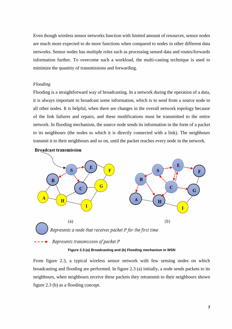
Flooding
Flooding is a straightforward way of broadcasting. In a network during the operation of a data,
it is always important to broadcast some information, which is to send from a source node to
all other nodes. It is helpful, when there are changes in the overall network topology because
of the link failures and repairs, and these modifications must be transmitted to the entire
network. In flooding mechanism, the source node sends its information in the form of a packet
to its neighbours (the nodes to which it is directly connected with a link). The neighbours
transmit it to their neighbours and so on, until the packet reaches every node in the network.
Figure 2.3:(a) Broadcasting and (b) Flooding mechanism in WSN
From figure 2.3, a typical wireless sensor network with few sensing nodes on which
broadcasting and flooding are performed. In figure 2.3 (a) initially, a node sends packets to its
neighbours, when neighbours receive these packets they retransmit to their neighbours shown
figure 2.3 (b) as a flooding concept.
8
3 State of the Art
3.1 Introduction to Routing Concept
Routing is the procedure in which data can be send to destination via selecting different ways.
Once the paths have been chosen, intermediate nodes are used to forward data traffic one end
point of the transmission to the other endpoint. Algorithms for routing are used for the purpose
to determine the "best" path closer to the destination in line with one or greater metric, build
upon on the requirements of the application. For instance, one broadly utilized metric chooses
the route with the minimal number of hops through midway nodes towards the destination.
Alternative metrics could use the best link quality and consumption of energy is very little.
Unequivocally, that connection quality could be considered by current sending power hops, for
instance: low sending power reachability achieves the node in 3 hops, which is more energy
efficient contrasted with one higher sending power hops.
The algorithms need to efficiently manage a constantly evolving topology, whilst forcing as
slight control of traffic overhead, which is vital for existing system. The transmission of the
messages are very expensive in terms of energy consumed. In order to transmit data in the
network, nodes must compute this will be done with the help of routing protocols. There are
numerous methods for doing routing inside WSNs. There are three noteworthy general
grouping of the routing strategies: (a) Proactive Routing, (b) Reactive Routing and (c) Location
based or Geographic Routing. [20]
Proactive protocols, determine the paths initially, if there is any on-going demand for
communication. They calculate the existing routing tables ahead of time and maintain
these routing tables through periodic "update messages". The Destination - Sequenced
Distance Vector Routing and Optimized Link State Routing are some the examples.
Reactive protocols on the other side, do not calculate the routing tables ahead of time.
In reactive routing protocols, a path to the destination is currently unknown when a
packet needs to be forwarded. These routes are then acquired by nodes on demand by
triggering a "route discovery" process. For instance, by presenting a route request packet
through the network and afterward wait for a response from the destination node. This
response might take some time to arrive which causes some delay for the other packet
to deliver. The overhead of few packets like control packets in this protocol is

9
specifically reliant on the amount of data traffic that is available in the network. A
reactive protocol does not need each and every node to store routes for the total network;
rather it is computed only for destinations to which the data traffic needs to be
forwarded. Route discovery follows the communication request. Examples of such
routing protocols are Dynamic Source Routing, Ad Hoc and on Demand Distance
Vector protocols.
Geographic Routing uses the information of location to make the routing based
decisions. This kind of Routing protocol is attractive because of its low energy footprint
and that it does not need to use any flooding scheme to identify and discover routes.
"Euclidean space" is a space where each and every node wants to have knowledge about
it location in that space and also the destination location. With this piece of information,
the further messages can be routed without the prior knowledge of the current network
topology or earlier route discovery which prevailed. Geographic Routing also includes
Greedy Face Greedy (GFG), SPEED and (GPSR) Greedy Perimeter Stateless Routing.
3.1.1 Routing Challenges and Design Issues in WSNs
Regardless of the uncounted uses of WSNs, these networks have numerous limitations, e.g.,
constrained energy supply, controlled computing power and confined bandwidth of the wireless
connections associating sensor nodes. One of the essential design desires of WSNs is to carry
out data communication while trying to prolong the lifetime of the network and to avoid
degradation of connectivity done by employing aggressive energy management strategies. The
layout of routing protocols in WSNs is stimulated by means of many difficult elements. These
factors need to be overcome earlier than efficient communication can be performed in WSNs.
Within the following, a range of routing challenges and issues in design that have an effect on
the routing manner in WSNs are mentioned.
Node deployment:
Node deployment in WSNs is an application which is finely structured and also influences the
performance of the routing protocol. The deployment here in Node deployment can either be
randomized or deterministic. The sensors are manually placed and data is routed via pre-
determined paths or not predefined routes. However, in the other node deployment namely-
random node deployment the sensor nodes are scattered randomly developing an infrastructure
in an ad hoc way.

10
If the final distribution results of nodes are not uniform, ideal clustering becomes necessary to
allow connectivity and to be able to perform energy efficient network operation. Uniform
distribution of nodes could also be clustered to forward only one message instead of many on
the shortest path.
Energy consumption without losing accuracy:
Sensor nodes can distribute their controlled delivery of energy by enhancing computations and
transmitting packets (data) in a wireless environment.
As such, energy preserving sorts of communication and computation are essential. Sensor node
lifetime indicates a robust dependence on the battery lifetime. In a multi-hop WSN, each node
performs a couple role as information sender and router. The breakdown of some sensor nodes
on account of power failure brings significant topological alternations and can require rerouting
of packets and redesign of the network.
Node/Link Heterogeneity:
In several studies, all sensor nodes were assumed to be homogenized, i.e., having identical
potential in terms of power, computation and communication. However, contingent upon the
application a sensor node can have distinctive roles. The presence of heterogeneous
arrangement of sensors raises many technical issues with packet routing. As an instance, few
applications may require a various mixture of sensors for monitoring humidity of the
surrounding environment, pressure, temperature and acoustic signatures by detecting motion,
and taking the image or video monitoring of moving objects. These unique sensors may be both
deployed independently or the distinct functionalities may be covered in the same sensor nodes.
At unique rates dissecting and reporting can be produced from the sensors, concern to numerous
service constraints, and can observe multiple information reporting models. For instance,
hierarchical protocols designate a cluster head node one-of-a-kind from the normal sensors.
These cluster heads can be selected from the deployed sensors or may be more powerful than
other sensor nodes in phrases of energy, bandwidth, and memory. Hence, the weight of
transmission to the BS is handled by way of the set of cluster-heads.
Fault Tolerance:
Some sensor nodes may moreover fail or be obstructed because of some interference from
surroundings, absence of power or physical harm.

11
The failure of sensor nodes ought to not tons affect the overall challenge of the sensor network.
In the event that numerous nodes fail, MAC and routing protocols need to suit the arrangement
of new connections and routes to the data gathering base stations. This could require actively
adjusting transmit powers and signalling rates on the prevailing links to reduce energy
consumption, or rerouting packets through areas of the network wherein extra energy is to be
had. Consequently, multiple levels of redundancy can be needed in a fault-tolerant sensor
network.
Coverage:
In WSNs, every sensor node obtains a certain view of the environment. A given sensor’s view
of the surroundings is constrained both in range and in accuracy; it may only cover a confined
physical region of the environment. Therefore, range scope is additionally a critical
configuration parameter in WSNs.
Scalability:
The quantity of sensor nodes deployed in the sensing area can be within the order of hundreds
or thousands, or greater. Any routing scheme should be able to work with this big quantity of
sensor nodes. In addition, sensor network routing protocols have to be scalable sufficient to
respond to events within the environment. Until an event takes place, most of the sensors can
continue in the sleep state, with data from the few remaining sensors, presenting a coarse
quality, may additionally increase sending energy to reach server/cluster center also if all nodes
dozing or could ensure all nodes are one hop far from the cluster.
Network Dynamics:
All most all the network architectures assume that sensor nodes are fixed. Routing messages
from node to node moving is extra tough since route stability becomes an important problem,
in addition to energy, bandwidth so on. Moreover, the detected phenomenon might be either
dynamic or static relying upon the utility, e.g., it is dynamic in an objective detection/tracking
utility. At the same time, it is static in forest monitoring for early fire prevention. Tracking static
activities, lets the network to work in a reactive mode, surely generating traffic while reporting.
Dynamic occurring of events in many applications require intermittent reporting and
consequently creates significant traffic to be routed to the BS.
12
Transmission Media:
Communicating nodes in a multi-hop sensor network are connected with the aid of the wireless
medium. The traditional issues related to a wireless channel (such as: high error rate, fading,)
may also affect the operation of the sensor network. In most of the cases, the required bandwidth
of sensor data will be low, in the order of 1-100 Kb/s regarding the transmission media is that
the design of medium access control (MAC).
One technique for MAC design for sensor networks is to apply TDMA primarily based
protocols that could need extra energy in comparison to contention based protocols like CSMA
(e.g., IEEE 802.11). Another technique like Bluetooth can also be used.
Connectivity:
In sensor networks with high node density, precludes them from being completely isolated from
each other. Therefore, sensor nodes are anticipated to be exceptionally connected. This,
however, won’t prevent the network topology from being variable and the sensor node failures
cause network size from being diminished. Similarly, connectivity relies upon the possibly
random or distribution of nodes.
Data Aggregation:
On account that sensor nodes might also generate vast, redundant data comparable packets from
more than one node can be aggregated in order that the variety of transmissions are decreased.
Data aggregation is the mixture of data from specific resources consistent with certain
aggregation characteristics, e.g., replica suppression, maxima, minima and average. This
method has been used to obtain energy efficiency and data switch optimization in some of
routing protocols. Signal processing strategies can also be used for data aggregation. For this
situation, it is referred to as data combination in which a node is capable of delivering a more
precise output signal by utilizing couple of techniques alongside with beamforming to join the
incoming signals and bring down the noise in these signals.
Quality of Service:
In few applications, information must be conveyed within a certain timeframe from the moment
it is detected, in some other case the information may be pointless. Consequently, bounded
latency for data delivery is every other situation for time-constrained applications.

13
However, in lots of applications conservation of energy, which is directly related to network
lifetime, is considered notably greater essential than the quality of data sent. As the energy gets
exhausted, the network might be required to diminish the quality of the outcomes so that we
can reduce the energy dissemination within the nodes by this reason the whole network lifetime
is prolonged. Subsequently, energy-aware routing protocols are required to capture this
requirement. Well Timed buffer can be used to decide how lengthy real time could be probably
still being available.
3.2 Shortest Path Algorithms
In topology the communications in a network is represented using a directed weighted graph.
The nodes in the network with their exchange components and the coordinated arcs in the graph
represents communication links between switching elements. The exchange components like
transmitter and receiver module for sending and receiving messages. Exchange elements could
be switch elements i.e. controller of bus switches and makes exchange of information.
Controller could also be kind of link and arc. Each arc has a weight that represent the cost of
sending a packet between two nodes in a particular course. This cost is generally a positive
regard that can inculcate such factors as deferral, throughput, error rate, monetary cost, etc. a
path between two nodes may experience through several intermediary arcs and nodes. The path
may timely or by condition changes so, that optimal trace can be focused. The goal is to briefest
way to find a route between nodes that has the smallest aggregate cost, where the aggregate
expense of a path is sum of the arc costs in that way.[24]
Dijkstra’s algorithm
Dijkstra's calculation is known as the single-source briefest path and the algorithm find the path
with the lowest cost (i.e. the briefest way) between that vertex and each other vertex. Dijkstra’s
algorithm uses metric as minimum distance. This algorithm searches for the shortest paths from
the source to all available nodes in the given graph. Its time complexity is O (|V | 2) but can
reach less than that when using priority queue. Dijkstra algorithm can’t handle negative
weights. But, it is asymptotically the fastest known single-source most limited way calculation
for self-assertive directed graphs with unbounded non-negative weights. It can likewise be
utilized for discovering expenses of most limited ways from a solitary vertex to a solitary
destination vertex by halting the calculation once the most limited way to the destination vertex
has been determined. It computes the duration of the shortest way from the source to each of
the left over vertices in the graph.

14
The single source shortest path problem can be depicted as takes after: Let G= {V, E} be a
coordinated weighted diagram with V having the arrangement of vertices. Edge Cost(e) be the
length of edge e, s will be the source and V is vertexes. The single source most limited way the
issue can be characterized as a requested pair G: = (V,E) with V is a set, whose components are
called vertices or nodes and E is a set of requested sets of vertices, called coordinated edges,
arcs, or arrows. For example, if the vertices of the graph speak to urban communities and edge
way costs speak to driving separations between sets of urban areas associated with an immediate
street, Dijkstra's calculation can be used to find the shortest route between one city and all
different urban communities. Subsequently, the briefest way is the wide use of network routing
protocols. Directed-weighted graph is a coordinated chart with weight connected to each of the
edges of the graph. [24]
Figure 3.1:Directed graph
Dijkstra's – In a Greedy algorithm greedy calculations are used in issue solving methods based
on actions to see if there is a better long haul procedure. Dijkstra's calculation utilizes the eager
approach to solve the single source shortest path problem. It over and over chooses from the
un-selected vertices, ‘v’ nearest to source ‘s’ and declares the distance to be the real briefest
separation from ‘s’ to ‘v’. The edges of v are then checked to look if their destination can be
reached by means of ‘v’ observed by the relevant outgoing edges.
Bellman Ford Algorithm
The Bellman-Ford calculation is a calculation that figures shortest paths from a single source
vertex to all of the different vertices in a weighted digraph. The Bellman-Ford calculation
belongs to the algorithms of the label-correcting type that deal with all labels for vertex
distances as temporary until the last iteration, then all labels are set to optimal values.

15
This algorithm gives a probability to tackle the shortest path issues in graphs with negative
lengths of edges. For the situation when a negative cycle is found, the calculation yields
falsehood as the result of its operation. It works in O(|V ||E|) time and O(|V |) space complexities
where |V | is the number of vertices and |E| is the number of edges in the graph. This algorithm
makes N − 1 emphases in which it checks an edges and the algorithm continues in an interactive
way, by starting with a bad estimate of the expense and then upgrading it until the right regard
is found.
The first estimate is: Taking a glimpse at all edges of the chart and redesigning the expense of
the nodes is called a phase. Unfortunately, it is not adequate to take a look at all edges just once.
After the first phase, the cost of all nodes for which the most limited way, just uses one edge
have been computed effectively. After two stages all ways that utilizes at most two edges have
been computed effectively, and so on. A shortest path that utilizes larger number edges than the
quantity of nodes would visit some node twice and thus forming loop (circle).
At the end of the algorithm, the shortest path to each node can be constructed by going in reverse
utilizing the ancestor edges until the beginning node is reached. A cheapest path had to use this
circle of operations infinitely often. So, the cost would be reduced in each iteration.
Floyd–Warshall algorithm
The Floyd–Warshall calculation is a calculation for finding shortest paths in a weighted graph
with positive or negative edge weights (yet with no negative cycles). A single execution of the
algorithm will find the lengths (summed weights) of the briefest ways between all sets of
vertices, however it does not return details of the paths themselves. Forms of the figuring can
likewise be utilized for finding the transitive conclusion of a connection, or most stretched out
ways between all sets of vertices in a weighted graph. The Floyd–Warshall algorithm only gives
the lengths of the paths between all arrangements of vertices. With direct changes, it is
conceivable to make strategy to reproduce the actual path between any two endpoint vertices.
The Shortest-path tree be figured for every node in Θ(|E|) time utilizing Θ(|V|) memory to store
each tree which allows us to efficiently reconstruct a route from any two related vertices. The
algorithm is likewise known as Floyd's algorithm, the Roy–Warshall algorithm, the WFI
algorithm or the Roy–Floyd algorithm. The algorithm above is executed on the graph given
below in figure 3.2:

16
Figure 3.2:Floyd–Warshall algorithm calculations
To distinguish negative cycles utilizing the Floyd–Warshall calculation, one can examine the
corner to corner of the way network, and the nearness of a negative number shows that the
diagram contains no less than one negative cycle.
Comparison of these algorithms:
Algorithm Negative edge Single source All sources Time complexity
Dijkstra No Yes No O(|E|+|V|LOG|V|)
Bellman-Ford Yes Yes No O(VE)
Floyd Warshall Yes No Yes O(V^2log V+VE)
Table 3.1:Comparison between shortest path algorithms
3.3 LEACH (Low-energy adaptive clustering hierarchy)
LEACH is a TDMA-based MAC conventional protocol, which is coordinated with clustering
and a straightforward steering convention in remote sensor systems (WSN). The objective of
LEACH is to bring down the energy utilization required to make and keep up groups with a
specific end goal (in case of /compared to direct point to point communication of nodes) to
enhance the lifetime of a remote sensor network. It is self-versatile and self-composed. The end
goal to upgrade energy in the system, nodes are chosen as cluster head circularly and
haphazardly [17].

17
The typical nodes called group individuals join the relating cluster head nodes on the premise
of the rule of the vicinity. Typical nodes sense information and send straightforwardly to the
cluster head nodes. The cluster head nodes get detected information, total the information to
evacuate repetition and combination processes are done and data send to the sink/base station.
So LEACH builds system lifetime by diminishing system energy utilization, and decreasing
number of correspondence messages by information accumulation and combination. Drain
convention utilizes round as a unit, each round is comprised of cluster set-up stage and
unfaltering state stage, with the end goal of decreasing superfluous energy costs.
With a specific end goal to accomplish the outline objective the key undertakings performed by
Leach are as per the following:
• Randomized revolution of the cluster heads and the
• Corresponding clusters.
• Global correspondence lessening by the neighbourhood pressure.
• Localized co-appointment and control for cluster setup and operation.
• Low energy media access control and Application particular information preparing.
Figure 3.3:Flow chart of LEACH protocol

18
Running Process of LEACH
The Leach operation is arranged into various rounds, and each of these rounds has
predominantly two stages: The Set-up phase and the Steady-state for information transmission.
Figure 3.4:LEACH Protocol process
The Setup phase:
In this phase, the nodes are divided into several clusters dynamically and a CH is selected
randomly among the cluster nodes for each cluster. At the same time as forming clusters, quite
a number in the range 0 to 1 is chosen randomly and the similar one is compared with a limit,
t(s). Whenever the chosen value is less than t(s), then the chosen node will become CH for that
round. If else, it will continue as member node of the cluster. The threshold t(s) is computed by
using equation. This selection making additionally involves the past history of the node having
acted as a CH earlier. Once various CHs are elected, advertisement messages are broadcast with
the aid of the CHs. These messages are heard through a number of the close nodes and find out
the presence of one or extra CHs. A node can pick one of the CHs, in case more than one CH
exist, based totally on the received signal strength indication. Each node sends a join request
message along with its ID to its chosen CH. By using CSMA a non-CH node can send join
request message with its ID. After the setup phase, each CH knows its members and their
respective node Ids.
Threshold t (n):
𝑇(𝑛) = {𝑝 (1 − 𝑃 (𝑟𝑚𝑜𝑑
1
𝑝))⁄ ,∧ 𝑛 ∈ 𝐺
0,∧ 𝑛 ∉ 𝐺
Where,
p is percentage (%) of the CH nodes among all the nodes, r is number of the round and G is the
accumulation of the nodes that have not yet been CH nodes during the initial 1/P rounds.
Utilizing this edge equation, all nodes will have the capacity to be head nodes after 1/P rounds.
The examination is as per the following:

19
Each node turns into a cluster head with likelihood ‘p’ when the round starts, the nodes which
have been head nodes in this round won't be head nodes in the following ‘1/P’ rounds, in light
of the fact that the quantity of the nodes which is equipped for head node will slowly diminish,
thus, for these remain nodes, the likelihood of being head nodes must be expanded. New cluster
heads are picked after ‘(1/P)-1’ round where all nodes which have not been head nodes will be
chosen with likelihood ‘1’, when ‘1/P’ rounds finishes, all nodes will return to the same starting.
Figure 3.5:LEACH data transmission process
The Steady-state:
This stage is for information transmission where typical nodes sense information and send this
detected information to their separate cluster head nodes. The preparation of data collection and
combing the information is done by cluster head nodes and information will be sent to the base
station. Steady state phase starts once TDMA schedule is shared (CH assigns its TDMA
schedule to the nodes bolstered by it). Essentially it is based on this plan a node sends it’s
detected and keeps data to its CH within the individual. As soon as a CH collects all the data
from its individual members, it evaluates the mixture of data of different nodes and its very own
information and sends the aggregate values to the BS. Generally, the steady state phase length
is longer than that of the setup phase. After each round, new CHs are elected.

20
Deficiencies in classical LEACH Protocol
Unreasonable cluster head selection:
LEACH protocol does not take residual energy of each node into thought for the choice of
group head node as every node has a square with the likelihood of getting to be cluster head. In
the event that low-energy node is being chosen as cluster head node, then the system comes up
short soon because of high energy utilization causes unfavourable to energy adjusting among
the system. This outcomes information misfortune and lower in survival time of the system.
Unreasonable distribution of cluster heads:
The arbitrary determination, calculation of cluster head nodes causes the problem of imbalance
in energy load. Distance variable is not considered in cluster formation because of which once
in a while big clusters and extremely class clusters exist at the same time in the network. The
more distance range between cluster head node and base station, progressively more the energy
utilization of that node.
More responsibility on Cluster Head node:
Data accumulation and sending of processed data to the base station in a single-hop are
performed by cluster head. Because of that cluster head nodes exhaust its energy too fast as
compared to typical nodes. Additionally, if a cluster head node fails, the entire nodes connection
will deplete their energy as well.
3.3.1 Descendants of Leach Routing Protocol
LEACH-A (Advanced Low Energy Adaptive Clustering Hierarchy):
The drawback to LEACH protocol is that the node which is acting as cluster head for a round
is consuming much more energy than others. This drawback of traditional LEACH is eliminated
by LEACH-A (LEACH - Advanced). In this heterogeneous energy convention is proposed with
the end goal of diminishing the node failure probability for increasing the lifetime of the
network or increasing time to first node die, or increasing the stability of the sensor network.
Each sensor knows the beginning of each round utilizing synchronized clock. Let ‘n’ be the
overall number of nodes and ‘m’ be the fraction of ‘n’ which have energy more than different
nodes referred as CAG nodes (nodes selected as gateways or cluster heads). The rest of ‘(1-
m)*n’ nodes would be acting as normal nodes. In Figure 3.6 a typical LEACH-A protocol is
shown [11].

21
Figure 3.6:LEACH-A protocol
Advantages of using LEACH-A protocol are:
Distributed Algorithm where cluster configuration is independent of the base station.
TDMA/CDMA methods save maximum energy by permitting clusters hierarchy of
diverse levels and CAG nodes will keep on sending information even after failure of
every single typical node.
LEACH-C (Centralized Low Energy Adaptive Clustering Hierarchy):
LEACH includes the uniformity as after some rounds the node have acted as cluster head and
thus does not guarantee the good cluster head distribution, to cover this drawback LEACH C
was proposed. It is a centralized clustering algorithm. Its steady phase is identical to LEACH.
However, its setup phase is as:
• Each node transmits its location information (possibly using GPS) and residual
energy to the BS.
• The optimal CH is computed and selected by BS.
The BS needs to be guaranteed that the energy load must be equally conveyed among all nodes
and to do this the BS system processes the normal typical node energy and figures out which
nodes have energy beneath this normal. Once the clusters and associated cluster heads are
computed, the BS broadcasts a message that consists of a cluster Head ID for each node. In
cases like the ID of the node matches with itself, then that node is CH node and its destination
is BS and if the ID is not quite the same as the node ID then, the node has to send the data to

22
the node, whose ID is given and if the node is not cluster head then it must decide its TDMA
slot for information transmission and goes to offline/sleep until it’s time to transmit data. The
benefits of this protocol over fundamental LEACH is the deterministic methodology of picking
the quantity of cluster head nodes in each round which is fixed at the time of deployment.
LEACH-C leads for higher distribution of cluster head nodes inside the network. Regardless,
LEACH-C needs current area data of all nodes utilizing GPS which is not robust.
Cell-LEACH (Cell Low Energy Adaptive Clustering Hierarchy):
In Cell-LEACH, WSN is separated into a several clusters where every cluster is further
partitioned into seven sections called cells. A few sensors are incorporated inside every cell
from which one sensor node is chosen as cell-head. No recalling and re-clustering is done once
deployed. Each cell node sends data to the cell head at its assigned time given by TDM. The
data collection capacity is performed by cell heads and prepared information are sent to cluster
heads. Cluster heads also performs the same function as cell heads and exchanges data to the
base station. After the first round, the cell head and the cluster head will be resolved
haphazardly. In this protocol, the sensing field is divided into cells and one node is chosen as
cell head among them. The clustering and the cell structures will remain same throughout the
life of the network lifetime.
Figure 3.7:CELL-LEACH Protocol

23
Cell head inside the cell accepts the data from the connected nodes by dividing the receiving in
TDM Slots. The cell head aggregates the data, removing the redundant data that were collected
from the connected nodes and then transmit that data to the Cluster head. The cluster head again
aggregates the data and transmit that data to the Base station (BS).
It uses two levels:
Cell head level and
Cluster head level.
MH-LEACH (Multi-Hop Low Energy Adaptive Clustering Hierarchy):
In LEACH protocol, the group head nodes send information to the base station directly,
irrespective of distance between them. If size of network is big in terms of distance between
CH and base station, this will leads to high energy dissemination of cluster head node. To
increase energy effectiveness of the convention, multi-hoping correspondence is introduced.
Firstly, nodes transfers sensed data to the cluster head and there is no direct transfer of packets
to base station by sensing node, transferring of sensed data to base station is done by cluster
heads. This protocol embraces an ideal way between the cluster head and the base station. MH-
LEACH requires extra Cluster heads indirections not Clustering on energy forming, best traces
from local gradient knowledge combined with Clusters on cluster able end regions, Inter Cluster
communication could be better with orientation instead of Cluster Center indirection sending,
energy overhead for repeated setup, on higher Cluster Level is the indirection much more wide
effort compared to direct gradient combined path, by principle for example: if 90 degree Cluster
indirection (as bad as one wants to construct) with 50℅ more way compared to direct ways
which will merge if reasonable by gradient so Cluster control trade of direct sending parallel
paths by sending to Cluster and then one message to next level cluster. MH-leach will not
provide good speed for urgent message like orientation dies while it is sub-behaviour of
orientated routing in case of delay tolerant messages.
TL-LEACH (Two level Low Energy Adaptive Clustering Hierarchy):
Unlike LEACH protocol where cluster heads send information to the base station specifically
in a single hop, two-level pecking is done in TL-LEACH protocol. The totalled information
from each group heads and the base station, rather than sending straightforwardly to the base
station.

24
The advancement of this protocol reduces data transmission energy. Cluster head nodes die
early contrasted with other normal nodes in the cluster or far away from the base station. TL-
LEACH improves energy capability by utilizing a group head node as a transfer node in the
middle of cluster head nodes. CDMA of TL-leach reduces usable error. Therefore, speed is
improved compared to other leach methods.
Compassion of different LEACH routing protocols
Clustering
routing
protocol
Scalability Distributed Hop
limit
Energy
efficiency
Homogeneous Use of
localization
information
LEACH Limited Yes Single
hop
High Yes No
LEACH-A Good Yes Single
hop
Very high No No
LEACH-C Good No Single
hop
Very high Yes Yes
LEACH-
Cell
Very good Yes Single
hop
Very high Yes Yes
LEACH-
Multi-hop
Very good Yes Multi-
hop
Very high Yes Yes
LEACH-
TL
Very good Yes Single
hop
Very high Yes No
Table 3.2:Comparison of various LEACH enhancement
3.4 Gradient Based Routing
The GBR (Gradient Based Routing) protocol is a variant of the Directed Diffusion protocol. It
is therefore a query-based routing protocol where information from a sensor node or a group of
sensor nodes is normally requested from the Base station (BS) by means of an interest message
that is broadcast on the network. The identified source node sends the requested information to
the sink (BS) via intermediate nodes. Its main concept lies in recording the number of hops
when a node receives the interest message [19].
25
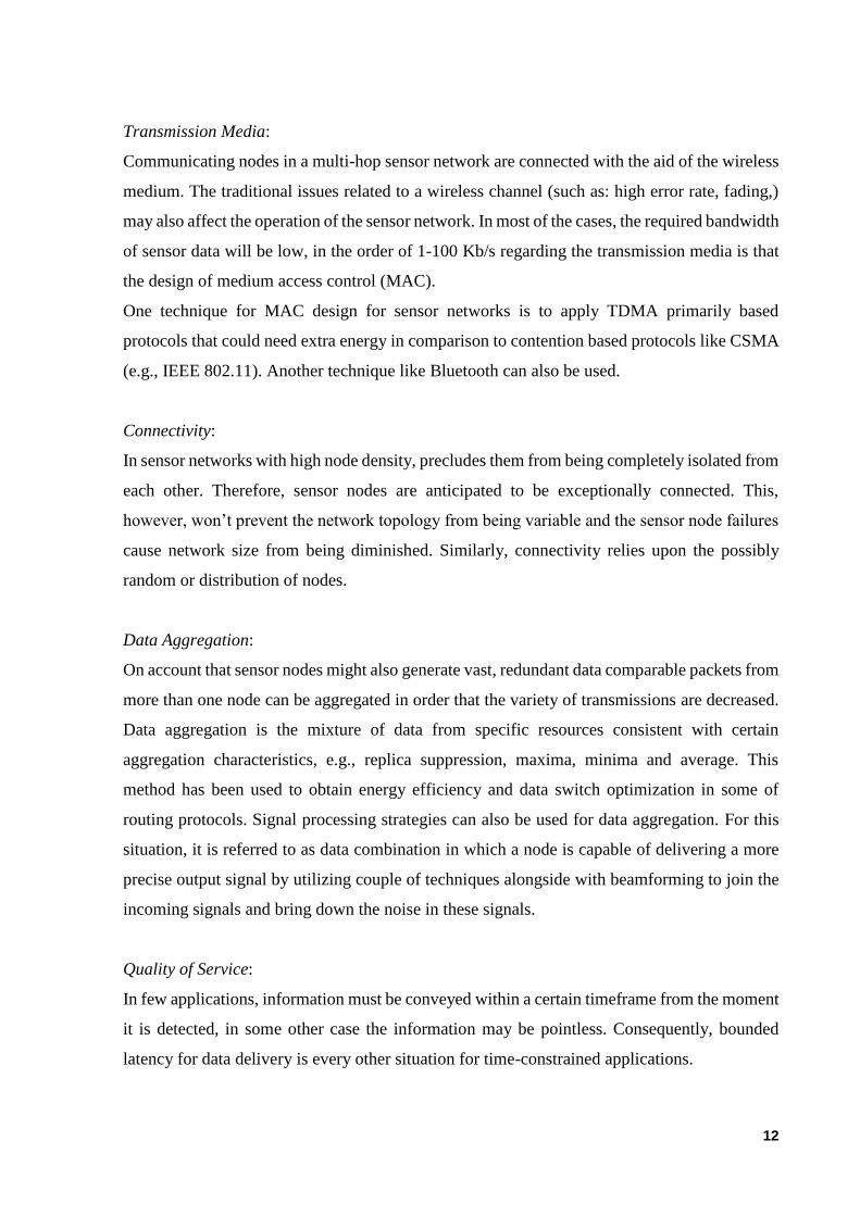
In this way, each node sets up its stature according to hops with the minimum number. The
difference of heights between a node and its neighbours is considered the gradient on that link.
The packet is forwarded on the connection with the biggest gradient, which implies that the
packet is always transmitted along the shortest path.
Figure 3.8:Simple gradient induced into a network
3.4.1 Overview: Improved GBR Techniques
GBR-C
GBR-C is a competing algorithm based on the GBR is to decrease the retransmission, so as to
spare the energy of the system. There are two queries that should be answered in this algorithm.
First of all, what number of candidate forwarders should be involved for each hop transmission.
Since receiving packets also consume energy, thus, broadcasting packets to all neighbours may
waste energy. Besides, the choice of the most proficient method to pick the best nodes to
forward the packets without duplication should be replied. Keeping in mind the end goal to
answer the query, the energy utilization for GBR is analysed to decide the number of candidate
forwarders. Accept that the force utilization of sending is Ptx while the energy overhead of
getting is Prx.

26
Assume that the information message size is M and the bit rate is Bitrate. The candidate
forwarders number is ‘n’. The transmission likelihood ‘p’ is referred to as the probability for
one link that the receiver gets the message effectively. [23]
Energy consumption of one hop transmission is:
𝐸 =(𝑃𝑇𝑋 + 𝑛 ∗ 𝑃𝑅𝑋)
𝐵𝑖𝑡𝑟𝑎𝑡𝑒(
𝑀
1 − (1 − 𝑃 𝑛))
n=1, 2,3,4,5
Figure 3.9:The energy consumptions of nodes in GBR-C
(ptx=65mw/sec, Prx=21mw/sec, M=800, Bitrate=19200bits/sec)
Assuming that the small, low-power sensors node power utilization model is used and ‘p’ is set
as 0.4 ≤ p ≤ 1, then the energy utilization for ‘n’ from 1 to 5 can be resolved. It can be seen that
energy can be spared on the off chance that we set n=2 for P<0.75. This could save up to 23%
power for one hop transmission. Moreover, it can likewise be seen that it is sufficient to set at
generally two candidate forwarders when 0.45 ≤ p ≤ 0.75. In general, probability should reduce
quality measure of link in case of retransmission, if it is small enough then automatically switch
to other node to forward. In GBR-C number of forwarders not in relation to later required
energy. For example 10 forwarder but only on one required, cases where two forwarders are
enough but much retransmissions are required. This issue can be overcome in methods
described in concept.
27
Transmission Probability Candidate Forwarders Number
P ≥ 0.75 n=1
P ≤ 0.75 n=2
Table 3.3:Candidate forwarder number
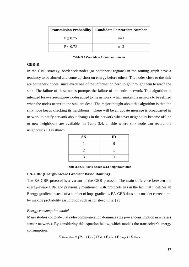
GBR-R
In the GBR strategy, bottleneck nodes (or bottleneck regions) in the routing graph have a
tendency to be abused and come up short on energy before others. The nodes close to the sink
are bottleneck nodes, since every one of the information need to go through them to reach the
sink. The failure of these nodes prompts the failure of the entire network. This algorithm is
intended for overseeing new nodes added to the network, which makes the network to be refilled
when the nodes nearer to the sink are dead. The major thought about this algorithm is that the
sink node keeps checking its neighbours. There will be an update message is broadcasted in
network to notify network about changes in the network whenever neighbours become offline
or new neighbours are available. In Table 3.4, a table where sink node can record the
neighbour’s ID is shown.
SN ID
1 B
2 C
3 D
Table 3.4:GBR sink nodes w.r.t neighbour table
EA-GBR (Energy-Aware Gradient Based Routing)
The EA-GBR protocol is a variant of the GBR protocol. The main difference between the
energy-aware GBR and previously mentioned GBR protocols lies in the fact that it defines an
Energy-gradient instead of a number of hops gradients. EA-GBR does not consider correct time
by making probability assumption such as for sleep time. [23]
Energy consumption model
Many studies conclude that radio communication dominates the power consumption in wireless
sensor networks. By considering this equation below, which models the transceiver’s energy
consumption.
E Transceiver = (PT X +PRX )∗T d +E Idle +E Sleep )+E Trans

28
Where, PTX and PRX represents the transmitted and the received powers respectively;
transmission’s time duration is Td on hop which is a probabilistic measure; Td is a random
variable. [25] The time duration Td of a successful transmission on a single link is random but
is function of the following deterministic parameters:
• Data size (M): This size is variable depending on the type of message being transmitted
which could be the interest message, data message or a control message such as
acknowledgement messages (ACK) etc. This quantity is usually measured in bits.
• Data rate (B): Also referred to as bit rate is usually measured in bits per second. In ideal
channel conditions the transmission’s time duration can be modelled as follows:
Td = M / B
Figure 3.10:EA-GBR process flow diagram

29
Figure 3.10, illustrates the process flow in the EA-GBR. The idea of the GBR-Competing
algorithm is to improve the probability of successful transmission by using multiple potential
hops instead of one, therefore reducing the probability of failure on a link as follows: For ‘n’
competing forwarding nodes the probability that none of the n candidate sensor nodes receives
the message reduces to(1 − 𝑃𝑠𝑡)𝑛. Therefore, the probability for successful transmission on n
candidate links is improved to:
𝑃𝑠𝑢𝑐𝑐𝑒𝑠𝑠 = 1 − (1 − 𝑃𝑠𝑡)𝑛
From figure 3.11, the average power consumption of all the three routing protocols seems to
converge around a probability of success of 0.75 and suddenly the energy efficiency
performance is reverted. The generic GBR followed by the EA-GBR performs better than the
GBR-C for higher probability of successful transmission.
This may be their low number of control overheads. For; WSN where the total energy
consumption is considered the EA-GBR is preferable as compared to the generic GBR and the
GBR-C. It also demonstrates that the aggregate energy of the network increases more or less
linearly with respective to the network’s scalability is observed. [23]
Figure 3.11:Evaluation of GBR techniques

30
3.5 Event Driven Routing Protocols
Event-to-Sink Reliable Transport (ESRT) Protocol
In this sink makes the choice primarily based on information collected from a number of source
nodes inside the region the wherein clearly the event passed off rather than individual sensor
nodes in the network. ESRT plays the event detection reliably based totally on reporting
frequency ‘f’ adjusting it below four network states and situations [31].
There are 5 kinds of ESRT actions associated network states are performed. First, is low
reliability with no congestion (NC, LR) in which f increases multiplicatively. Next one is high
reliability with no congestion (NC, HR) in this factor f decreases conservatively. Third one is
high reliability with congestion (C, HR) where f may be multiplicative but in general its value
decreases. Next is low reliability with congestion (C, LR) here exponentially decline in f value
and finally, optimal operating region (OOR).
Benefits of ESRT: Sink only collects information, i.e. quantity of source nodes within the event
coverage location and offers numerous levels of reliability primarily based on network
conditions information to the sink. The negative aspects of ESRT are that it follows a central
control strategy which is not an energy productive technique and the sensor field with numerous
event happening at the identical time the alteration off for all the sensor nodes will not result in
better performance because the events are unbiased of each other and moreover the event going
on region won’t be same.
Congestion and Delay Aware Routing (CODAR) Protocol
The principle objective of CODAR is to upgrade the unwavering quality and the timeliness of
the information transmission via critical nodes through the utilization of congestion avoidance
and mitigation. CODAR issue of data rate adjustment, so information lost instead of
compressed overview offered, requires location information. Two categories which classifies
CODAR protocol are: [26]
• Critical nodes: The nodes nearer (offers greater significant data, critical data generating
nodes) to the event
• Regular nodes: When there may be no event sensing occurs the critical nodes become
regular nodes. The CODAR has focused on two mechanisms which are end-to-end
delivery delay management and congestion avoidance.

31
Congestion avoidance: Each node in the locale where the occurring of event is been broadcasted
to its location and Relative Success Rate (RSR) value in fixed interval using control packets.
The RSR allows to keep away from congestion through selecting lightly congested nodes. End-
to-end delivery of information management deals with energy exertion of spreading node’s
postponement to previous nodes and no prioritization, higher of critical messages i.e. to forward
just present message from buffer in congestion circumstance, so that lower critical reliability
can be achieved. In the CODAR, each essential node transmits their critical information packet
with the cut-off to the sink with a header. All the node in the middle checks this header field
before transmitting the packet, and if the intermediate node has end-to-end postpone that can’t
meet the time limit then the packets were been dropped by the intermediate node .
Advantages of CODAR: CODAR delivers a high amount critical data within a specified amount
of delays and CODAR has a potential to reduce the congestion by avoiding congested nodes
during the selection of route and also by dropping packets. Disadvantages of CODAR include
such as, not suitable for a large number of critical nodes and less energy efficient.
Event Reliability Protocol (ERP)
The ERP performs solid transmission of information containing event related data while
minimizing excess packets. The ERP convention makes usage of verifiable affirmation (iACK)
mechanism remembers the decision objective to accomplish the unfaltering quality. The ERP
operation depends on mechanism called Region based particular retransmission component in
which, when the sensor node detects an occasion, it will then send the recognized occasion data
to the following next node and after that this next hop node stores that event information in its
buffer and the data at the head of its buffer is transmitted to the following next hop node. At the
point when the node hears that the following next node is transmitting the packets that was sent
by it, then it is known as an implicit acknowledgement for telling that the packets is sent
successfully. And the node, then deletes the passage of the packets from the line end and the
following packet in the line is processed. The region based particular retransmission makes
utilization of the source ID, source location and event’s time as an opportunity as a wellspring
of a specific parcel which is to be retransmitted. The separation between the nodes is measured
to check whether they are in the scope of each other. If there is another packet for the same
occurring event area sends, then that packet is sent to the sink else's the main packet is sent
again until a packet from the same event area. [29]
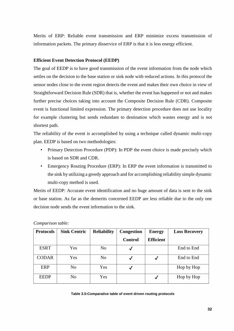
32
Merits of ERP: Reliable event transmission and ERP minimize excess transmission of
information packets. The primary disservice of ERP is that it is less energy efficient.
Efficient Event Detection Protocol (EEDP)
The goal of EEDP is to have good transmission of the event information from the node which
settles on the decision to the base station or sink node with reduced actions. In this protocol the
sensor nodes close to the event region detects the event and makes their own choice in view of
Straightforward Decision Rule (SDR) that is, whether the event has happened or not and makes
further precise choices taking into account the Composite Decision Rule (CDR). Composite
event is functional limited expression. The primary detection procedure does not use locality
for example clustering but sends redundant to destination which wastes energy and is not
shortest path.
The reliability of the event is accomplished by using a technique called dynamic multi-copy
plan. EEDP is based on two methodologies:
• Primary Detection Procedure (PDP): In PDP the event choice is made precisely which
is based on SDR and CDR.
• Emergency Routing Procedure (ERP): In ERP the event information is transmitted to
the sink by utilizing a greedy approach and for accomplishing reliability simple dynamic
multi-copy method is used.
Merits of EEDP: Accurate event identification and no huge amount of data is sent to the sink
or base station. As far as the demerits concerned EEDP are less reliable due to the only one
decision node sends the event information to the sink.
Comparison table:
Protocols Sink Centric Reliability Congestion
Control
Energy
Efficient
Loss Recovery
ESRT Yes No ✔ End to End
CODAR Yes No ✔ ✔ End to End
ERP No Yes ✔ Hop by Hop
EEDP No Yes ✔ Hop by Hop
Table 3.5:Comparative table of event driven routing protocols

33
4 Concept
This chapter deals with the concepts for implementing the proposed routing technique. In this
there are three rules. Mainly rule 1 and rule 2 are for achieving the aim of the thesis and rule 3
is developed for industrial application scenarios. The proposed routing, flow relies on the
following main concepts: (1) Shortest path routing and (2) Energy path routing. The gradient is
also assigned for each sensing node. This thesis project is implemented in OMNeT++ based on
C/C++ with MiXiM framework to achieve wireless properties.
4.1 Energy Shortest path observing module
In this section, how rule 1 and 2 are used to achieve the goal. For brief understanding of rule 1:
In networking, the path between source and destination is calculated based on number Hop
count. Data packets pass through different network elements such as, bridges, routers and
gateways on the way. A hop occurs every time when packets are been send to next following
node by sending device/node. Increase or more number of hops between source and destination
leads lower real time performance. For measuring distance between two hosts, Hop count are
used. This principle is considered for shortest path route in our network. Figure 4.1, gives brief
idea of hop count calculation.
Figure 4.1:Hop count of a simple network

34
For understanding of energy based routing is explained in chapter 3. In rule 1, both routing
techniques are used, where a switch is defined in order to perform switching between both the
techniques. The energy delta is a parameter which defines the switch weight value, in our case
25 is considered. This means sending node compares the energy levels of its neighboring nodes
if the difference between two nodes is less than our defined value, i.e. 25, then routing will be
based on hop count method (shortest path) and in case of the energy delta value is greater 25
which implies that difference of energy level of its neighbors is high therefore by our rule it
routes its messages by energy based routing technique.
Figure 4.2:Rule 1 Implementation
4.2 Rule for rate of delivery improvement
Now, rule 1 is further improvised, adding a concept for considering the number of messages
delivered at the server end. This rule will improve the rate of delivery of the messages in the
network. Moreover, rule 2 is improvised version of rule 1 with respect to the network lifetime.
Hereafter the energy delta checks if value is less than 25 in our case it follows shortest path, if
value is more than 25 than we check for special condition in order to decide further routing
scheme to implement into the network.
The condition is:
Deltamsgs < Sendmsgcnt/2
Deltamsgs is variable to determine further routing decisions. This condition check is done after
satisfying the condition of energy delta greater than 25.

35
In this condition it checks for the message count. If the message count is half or less than half
when compared to previous period messages received, then it switches to other routing
technique. For better rate of delivery of messages at the server.
From figure 4.3, how these rules incorporated into one with observer condition. After the check
of delta message variable, now routing is decided. If the conditional check is not satisfied (No)
then energy path is used for transmitting messages. If the condition is satisfied (yes) that is delta
messages are less than the half of the send message count than switching between paths will
take place. For example, before the check condition shortest path is used than after it justifies
the check condition it will switch to energy path and vice versa. By this we can rotate using
these routing techniques instead using only one routing method.
Figure 4.3:Rule 2 Implementation
Energy
Check

36
Summarizing:
Rule 1 is for implementing two routing techniques with energy check condition to
choose one of the routing methods to implement.
Rule 2 is for improving the number of messages delivered at the server end. With this
rule network energy is balanced by using different routes to reach the server. Therefore,
we can use nodes energy in a much more balanced way and network lifetime also can
be improved.
4.3 Brightness Event Observing Module
For industrial applications another rule is used along with rule 1 and 2. In this rule an event
based observation is performed in a scenario. Here brightness is an event which has to be
observed to inform the base station about the situation. For an instance, a logistic industry is
considered where we are having a conveyer belt for unloading or loading packages/boxes, along
with the belt there are some sensor placed for different purposes to report it to central
monitoring unit (server).
Figure 4.4:Industrial implementation: Rule 3

37
To illustrate how it is implemented, we have to consider figure 4.4 scenario, where boxes are
moving on the conveyor belt with a sensor to perform certain sensing tasks like the weight of
the package, scanning barcodes, etc. and with this sensor one light emitting source connected
to it and one sensor is connected to the server. The main purpose of the light is whenever an
event is occurred light should go ON and it will be tracked by the camera. User feedback error
lights can be reused for error detection in server with a camera. Counting goods camera can be
used for the light detection purpose. The sensor which is connected to the server used for
stopping the conveyor belt being operational. A server with a camera attached to it for purposes
of tracking events generated by sensors. Raspberry pi can be used as camera in this case. When
a sensor triggers an event in case like wrong barcode or the damaged box light goes ON. This
light will be traced by the camera mounted to the server, then the server will stop the process
by a sensor connected to the server. By these situations can be controlled in industries.
Raspberry Pi
The Raspberry Pi is a small size computer board available with a processor, RAM and some
hardware ports. It is used to track bright spots in a scenario in our case a light is used for
brightness generation, to track this light raspberry pie is used. The run time parameters obtained
in a number of image frame slots, for example, for the first 100 frames and then set these
parameters to zero. The next run-time parameters result obtained for 200 frames and then next
300 frames. The number of image frames are being increased to gain the average frame per
second. The number of frames are increased 100 plus previous slot of frames.
Figure 4.5:Raspberry pie and Tracking bright spots

38
Figure 4.5, shows the tracking of bright spots by the raspberry pie camera. Here we can notice
circles which represent bright spots and it can be used for tracking objects with in motion. The
green colour line shows the movement of the bright spot, in this case it moved to left.
4.4 Observer Components
4.4.1 Update Timer
It is a periodic timer to update network for any topological changes. This timer is activated by
the server itself, for our network it is defined that every T=10ms an update message is
broadcasted by the server in the network. After listening to this message from server nodes will
asks for a response from its neighbours to know whether its neighbours are active or not. This
update timer can be defined based on the size of the network.
4.4.2 NeighboursResponse
At the initial stage of routing, all nodes broadcast neighbour response messages in order know
their neighbours. After that at every update timer sensing node will once again broadcast the
neighbour response. By this neighbour response message a routing table can be constructed in
that table it consists of information about its neighbouring nodes energy level, gradient value
and hop counts to reach the server. In cases like connectivity loss with its neighbours, after
getting update timer message from the server nodes sends response message to its neighbours.
When the response from its neighbour, which is previously present does not send any neighbour
response message back than this node can update its routing table by removing that node.
4.4.3 Weight Update
This parameter will decide how long the network is operational. Weight update varies with
different network topologies. In this thesis work weight is defined by difference observed in the
messages received at the server when compared to previous interval. In our case, check
condition in the rule 2 is the weight factor. Weight can be managed or assigned depends on the
size of the WSN. While defining weight factors to be considered like number of nodes in the
network.
4.4.4 Node Setup
While implementing node in the simulation environment, a node should have following
information such as: information about its neighbour which consists of their energy level,
gradient value and it also consists of its own gradient value and energy level.

39
Figure 4.6:Node setup
The above figure 4.6, shows with the nodes having various information with it. While
considering one node for example node 4 which is having 3 line of information:
First line is about information about node 4 itself: in which ‘49’ represents ID of the
node in the network, ‘g13’ is the gradient with value 13, ‘e100’ gives energy info which
means node 4 has energy of 100, ’o’ is number of old messages, ‘n’ is number of new
messages, ‘d’ is a delta variable which difference between both old and new messages.
And ‚‘s‘denotes message count variable value.
Second & Third line are information about its neighbours. For instance, in second line
it has ‘31’ which is ID of its neighbour, ‘13’ is gradient value with respective to the
node 4 (i.e. gradient value of its neighbour -1) and ‘31/100’ represents node with whose
ID is ‘31’ having energy of ‘100’. Third line also similar to the second line.
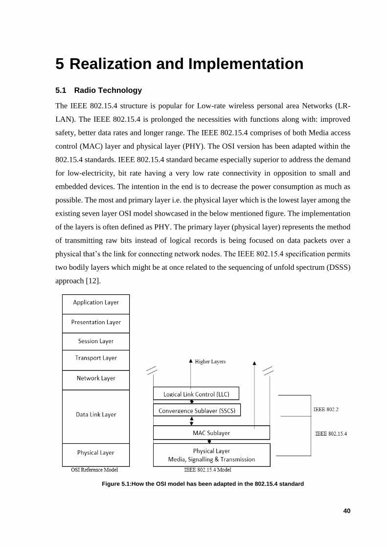
40
5 Realization and Implementation
5.1 Radio Technology
The IEEE 802.15.4 structure is popular for Low-rate wireless personal area Networks (LR-
LAN). The IEEE 802.15.4 is prolonged the necessities with functions along with: improved
safety, better data rates and longer range. The IEEE 802.15.4 comprises of both Media access
control (MAC) layer and physical layer (PHY). The OSI version has been adapted within the
802.15.4 standards. IEEE 802.15.4 standard became especially superior to address the demand
for low-electricity, bit rate having a very low rate connectivity in opposition to small and
embedded devices. The intention in the end is to decrease the power consumption as much as
possible. The most and primary layer i.e. the physical layer which is the lowest layer among the
existing seven layer OSI model showcased in the below mentioned figure. The implementation
of the layers is often defined as PHY. The primary layer (physical layer) represents the method
of transmitting raw bits instead of logical records is being focused on data packets over a
physical that’s the link for connecting network nodes. The IEEE 802.15.4 specification permits
two bodily layers which might be at once related to the sequencing of unfold spectrum (DSSS)
approach [12].
Figure 5.1:How the OSI model has been adapted in the 802.15.4 standard

41
• In Europe, 868-868.8 MHz is used. Which allows one correspondence channel.
• In North America, 902-928 MHz is used. In which it has up to thirty correspondence
channels.
• The overall use is 2400-2483.5 MHz, up to 16 channels.
The physical layers are regularly categorized into the 868/915 MHz groups with exchange rates
of 20 and 40 Kbit/s, and the 2450 MHz band with a rate of 250 Kbit/s.
Access to the physical radio channel is controlled by the MAC layer. Because of the fact the
physical radio channel is shared among all the senders and collectors in the area of each diverse,
the MAC layer provides a mechanism to choose while the radio channel is idle, and when it is
safe to send messages. Carrier sense multiple access with Collision Avoidance (CSMA/CA) is
used to determine while it's safe to send messages. If a node desires transmit information, it
ought to first listen to the channel for a prearranged amount of time. The reason is to decide
whether or not or other node is relaying at the channel within the remote reach. If the channel
is sensed "idle", the node is authorized to start the transmission technique. I f the channel is
distinguished as "busy" the node concedes its transmission for a random timeframe. IEEE
802.15.4 does no longer experience the channel constantly because of power limitations.
Instead, the station begins sensing the channel best at the same time as the back off timer reaches
0.
Power Consumption: The energy usage of IEEE 802.15.4 is dictated by the current draw of the
electrical circuits that enforce the physical correspondence layer and by means of the measure
of time throughout which the radio is turned on. There are several methods a radio can preserve
communication abilities at the same time as it is switched off.
Figure 5.2:Power consumption of the CC2420 IEEE 802.15.4 radio transceiver

42
Figure 5.2, shows the power consumption of the CC2420 IEEE 802.15.4 transceiver, as reported
by the CC2420 information sheet. It exhibits that the idle power utilization is significantly lower
than both the listen and the transmit power usage. However, in the idle mode the transceiver
will not receive any data. The former relies on upon the yield power, which is configurable by
means of programming on a per-packet basis.
5.2 OMNeT++
Introduction
An integrated development environment is based on the Eclipse platform and extends it with
new wizards, editors and several other extra functionalities. This platform is called the
OMNeT++. OMNeT++ provides a few functions for developing and configuring models (ini
and NED files), to perform batch executions, and analysing simulation results, whereas Eclipse
gives C++ editing, SVN/GIT integration and completely different non-obligatory functions
(database access, Bug tracking integration, UML modelling) with numerous open-source and
commercial plug-ins. OMNeT++ gives infrastructure and tools for writing simulations [2].
Figure 5.3:OMNeT++ GUI during simulation

43
One of the primary factors of this infrastructure is a component for simulation. From reusable
components and termed modules, models are assembled. Elegantly composed modules are
without any problem reusable, and can be joined in various ways. Modules can be associated
with each different through gates (different systems could name them ports) and combined to
form compound modules. The intensity of module nesting is not restricted. Modules
communicate through message passing, in which messages can also bring arbitrary data.
Modules can pass messages alongside predefined paths via gates and connections, or directly
to the destination, the occurring event is useful for wireless simulations, for example. Modules
may also have parameters that may be customized on module behaviour and/or to parametric
the model’s topology. Modules on the last level of the module hierarchy are referred to as simple
modules, and that they encapsulate the model behaviour. Simple modules can be programmed
in C++, and can make use of the available simulation library. OMNeT++ simulations may be
run under many extraordinary user interfaces. Animation, graphical user interfaces are very
beneficial for demonstration and debugging, and command-line user interfaces are better to
perform batch execution. The simulator as well as user interfaces and tools are extraordinarily
unbiased and portable. They are examined on the most common operating systems (Linux, Mac
OS/X and home windows). OMNeT++ uses several techniques for communication exchange
among partitions of a parallel distributed simulation, for instance MPI. The parallel simulation
set of rules is easy to extend, or new ones can be plugged in. The models do not want any unique
instrumentation to be run in parallel. OMNeT++ may even be used for clear presentation of
parallel simulation algorithms, as simulations can be run together, even beneath the GUI will
provide precise feedback on what is going on. [4]
Overview of OMNeT++
Modelling Concepts:
Message passing is way of communication in modules of an OMNeT++. The active modules
are termed simple modules; programming language used in OMNeT++ is C++ and simulation
class library files are used to implement the models. Simple modules are often classified into
compound modules, the number of hierarchy levels is limitless. Messages are sent either
through the links that traverse modules or straight-away to different modules.

44
NED Language:
NED (Network Description) Overview
NED is the topology description language of OMNeT++. It has a primary, simple structure yet
it is capable when it comes to defining normal topologies, that are chain, ring, mesh, tree, and
so on. NED language is used to define the structure of a simulation model by user. NED lets
the user a chance to claim simplified modules, connect and assemble them into compound
modules. The user can label a few compound modules as structures, networks that are
independent simulation models. Channels are any other component type, whose examples can
likewise be utilized as part of compound modules.
Hierarchical
Hierarchies are introduced to deal the complexities which traditional way. A single entity which
would be excessively unpredictable can be broken down into several small modules and these
are used as a compound block.
Component-Based
Simple modules and compound blocks are inherently reusable, which not only reduces code
redundancy, but more importantly, it allows component libraries (like the INET Framework,
MiXiM) exist.
Interfaces
Module and channel interfaces can be utilized as a placeholder where typically a module or
channel sort of can be used and the specific module or channel type is resolved at the network
setup time by a parameter. Specific module types need to actualize the interface.
Inheritance
Modules and channels can be sub-classed. Derived modules and channels might add several
parameters, gates, and (in the case of compound modules) new sub-modules and connections.
Gate size of a gate vector and some existing parameters to specific value are been set. [34]
Packages
The NED language has a Java-like package structure, to reduce the risk of name clashes
redundancy between different models. NEDPATH (familiar to Java’s CLASSPATH) has also
been introduced to make it easy to relate dependencies among different simulation types.

45
The NED Editor
Both graphical or text mode files of NED can be edited in the NED editor and additionally
irrespective of time the user can switch between the two modes. By switching between tabs at
the bottom of the editor window.
Figure 5.4:The Ned editor in Graphical mode
One of the advantage in graphical mode is that user can make compound modules, channels,
and other different component types. Graphical features that can be edited, icon sizing and
colouring, transmission range, and many others. The type and structure of NED files shown in
the Outline View with both graphical and text editing mode and also allows navigation to other
views. The Module Hierarchical View and the NED Parameters View can also be used with the
NED Editor (they will display the sub-module hierarchy and the parameters of the selected
module or sub-module) these views will be described by the Ini File Editor. Further related
views the Problems (which displays errors and warnings in NED files, etc.), and Task View
(which shows a list of all "todo" items found in NED files and other source files)

46
Simulation Launcher
The OMNeT++ IDE makes it possible to run simulations from the integrated environment. It is
possible to run a simulation as a normal C/C++ application and compiles with C++ source-level
debugging on it. The user can also run it as an only application or run batches of simulations to
find where runs differ in module parameter settings.
Process View
The Progress or Process View reports the status of simulation execution when you have a long
running simulation, or you are executing few runs in a batch. It is possible to cancel the
complete the batch operation with a single click, if necessary. IDE will not be blocked as
simulations are runs in separate processes. Therefore, user have an advantage to work parallel
while simulation is going in background.
Console view
Within the console view console buffer gets results from each and every running process. By
this user can access or analyse outputs after simulation is done. Console view menu or toolbar
helps in switching between console buffers or just clicking on debug view. [34]
Debug view
It is another Eclipse's standard Views, this will not only for finding bugs, it will display the
process which are completed and also with their exit codes. Processes are marked with run in
many numbers and launch times for easier identification. How the output is processing can be
known by clicking an item in the Console View.
Scave (Result Analysis)
The Scave is the result analysis tool of OMNeT++ and it helps in visualizing simulation of the
user process and results can be stored in the vector and scalar files. By this Scave user can work
equally well on the output of a single simulation run (one or two files) and the result of
simulation batches. In addition to systematic and repeatable processing, Ad-hoc is supported
for browsing of the data. All processing and charts are stored as “recipes”.
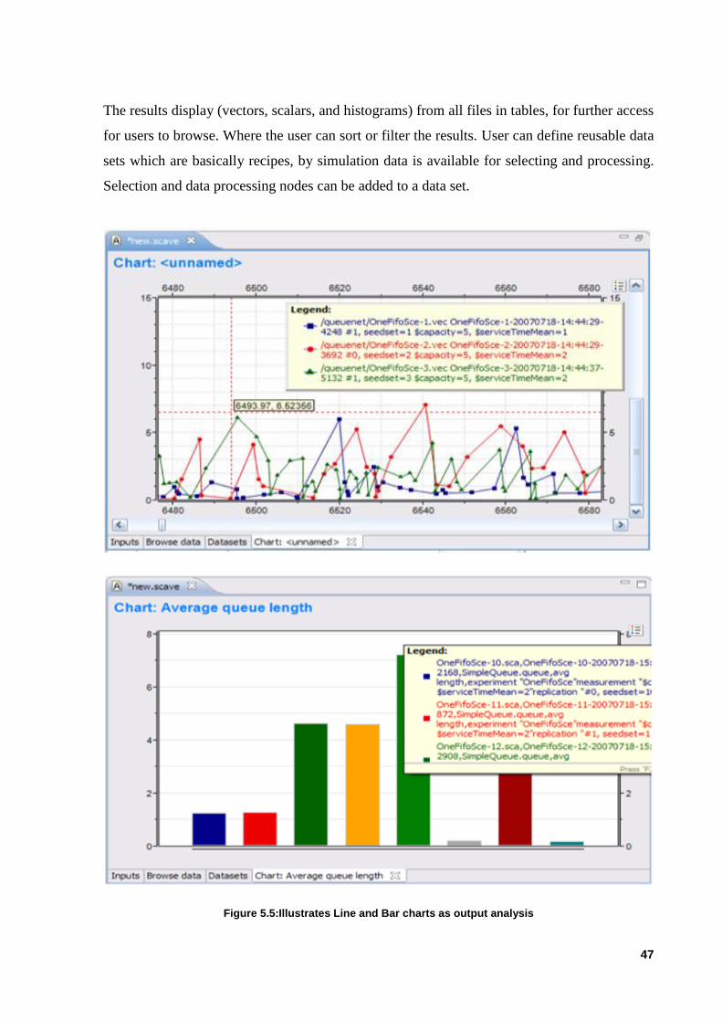
47
The results display (vectors, scalars, and histograms) from all files in tables, for further access
for users to browse. Where the user can sort or filter the results. User can define reusable data
sets which are basically recipes, by simulation data is available for selecting and processing.
Selection and data processing nodes can be added to a data set.
Figure 5.5:Illustrates Line and Bar charts as output analysis

48
Other Simulation Software Comparison:
Ns-2
NS-2 is the most popular network simulator utilized by researchers and it is an open source. It
is a discrete-event simulator written in C++ and is based on two languages: where C++ is used
to increase the simulator (i.e. to outlines protocol behaviours), and OTcl, associate object-
oriented extension of Tcl, which is used for manipulation of existing, periodic or triggered
actions, scenario configuration, C++ objects, etc. In NS-2, presentation and session layers are
excluded of the OSI layers. It has a huge pool of available features, which offers an extensive
number of external protocols. With the complex structure of the simulator, adding of new
components are hard assignment since it requires a decent knowledge of the simulator.
Similarly, with all discrete-event simulators, unique timing simulation (i.e. of code execution)
is impractical, in spite of the fact that a timing model can be included into the simulation. NS-
2 makes uses TCL for scenario generation, this lets complicated situations to be created
consequently by means of scripts. TCL commands control the simulator. Initially, based
computer networks NS-2 only supported simulation of fixed TCP/IP. [22]
Figure 5.6:Simplified view of Ns-2
In NS-2 there has been demand mobility, since standard NS-2 used for fixed network with their
devices are not moveable therefore extensions are required to achieve mobility in NS-2. It is
also difficult to mix wired and wireless nodes in the same NS-2 simulation. Nodes in NS-2 are
impressively more advanced than the sensor node which is typical. However, now simulation
of mobile ad-hoc network is supported. NS-2 supports DSDV, TORA for Ad-hoc routing and
AODV protocols. Free-space, shadowing and two-ray ground reflection are supported by
propagation models and also simple energy modelling is supported, this track the energy
utilized for each packet transmitted and received.

49
Models that are contributed gives support for other protocols (e.g. IEEE 802.11 and IEEE
802.15.4). In simulation scenario, while composing one needs to build a binding between OTcl
and the actual C++ classes by writing C++ classes for each one of their corresponding OTcl
class. It additionally permits defining disturbances and corruptions that may happen in a
simulated network like link interruptions, recovery by modifying scenario scripts and node
stoppage. Using Nam with NS-2 simulations can visualized, this could be done by traffic and
movement patterns generation and configuring OTcl code with these references as inputs.
OPNET (Optimized Network Engineering Tools)
This is commercial discrete-event simulator. It provides all kinds of wired and wireless
communication networks and distributed systems for the global environment to model, simulate
and evaluate performances. In this simulator practical scenarios can be designed by user with
various designing protocols and technologies.
The OPNET environment incorporates graphical tools for data analysis and data collection,
scenarios and scenario simulation. A project including a set of scenarios are represented within
the OPNET simulation. The OPNET central interface is responsible for creating the projects
through the project editor, from this editor all the accessible functionalities can be accessed and
also provides an access to other editors that propose functions including building packet
formats, node and process model creation and creating filters and parameters. Due hierarchical
modelling in OPNET a network is represented as a collection of sub-models with sub-networks
or nodes. The topology utilized as a simulation can be manually created, imported or selected
from the pool of predefined topologies, four level structure hierarchical way models are
developed. Network level, which handles topology modelling and overall configuration which
is not the OSI layer. OPNET gives numerous additional functions including a High-Level
Architecture (HLA) module, for allowing communication between various simulators. There
are three domains for modelling is done within the modelling environment: the communication
network topology to simulate is defined in network domain, the elements which are connected
to the network can send and receive data. Every module that described in the process domain
with their processors or queues. [22]

50
Figure 5.7:OPNET Modeler’s editors shown hierarchically
Comparison of Simulation software’s
Wireless sensor network simulation software is categorized in two kinds: commercial and non-
commercial. Non-commercial software are Parsec, NS2, Ptolemy, NetSim++, and C++Sim and
Commercial software are OPNET (OPNET Technologies, Inc.), EcoPREDICTOR. Out of all
these software's NS2 is the most popular one in non-commercial and OPNET is well-known in
commercial software. In this section we compare OMNET++ with other simulation software:
NS2 and OPNET [38].
Programming Model and Simulation Library
Coroutine/Thread-based programming models are generally used. While OMNET++ is
supported with both programming models. Although OMNET++, NS2 and OPNET are all
having strong Programmability. In case of simulation library, the OPNET simulation library is
based on C and NS2 simulation library provides less functions. While OMNET++ is a C++
class library which makes OMNET++’s functions are much more effective than NS2, C++ is
superior to anything C in WSN simulation.

51
Protocols and Models
OMNET++ uses protocols and models like TCP/IP, SCSI and FDDI and the model library
additionally rapidly culminates and it can fulfil the large-scale sensor network simulation.
Whereas in OPNET we get lot of protocol models including TCP/IP, ATM, Ethernet, etc. so
forth, yet it is so expensive to get the license. NS2 mostly centred on TCP/IP, which limits NS2
in WSN simulation. OMNET++ has the huge favourable in the model library and the accessible
model perspectives.
Network Topology and Hierarchical Models
NS2 utilizes Tcl to define its network topology. This permits critical adaptability in building
the topology, yet it moreover difficult to make a graphical editor, made it an inconvenience,
particularly for beginners. Moreover, NS2 does not permit hierarchical model, it significantly
restrains NS2 use in WSN. OPNET allows hierarchical models with arbitrarily deep nesting, as
OMNET++. A huge contrast between OMNET++ and OPNET will be OPNET models
dependably utilize fixed topology, while OMNET++’s NED and its graphical editors permit to
alter topology and parameterized topologies. In network topology and hierarchical models,
OMNET++ is superior to NS2 and OPNET.
Debugging and Tracing
One of the important issues in WSN are Efficient debugging and tracing. For debugging
purposes: there are tools like automatic animation, module output windows and object
inspectors in OMNET++. Most of the simulation software is supported by Automatic
animation. Moreover, different programmable simulation tools did not have object inspectors
and module output windows because of this they lack of a graphical runtime environment.
Simulation debugger in OPNET has a powerful command-line, even though it does not have a
graphical runtime environment. In WSN simulation NS2 is moderate. Mai n drawback of NS2’s
is that it requires a long time for execution and also not excellent by performance in bugging
and Tracing. In area, both OMNET++ and OPNET display good overall performance, due to
lack of graphical runtime environment, OMNET++ is more helpful to user than OPNET.[38]
Conclusion
OPNET requires significant time to learn to use it and has a convincing analysis and a way of
presenting the results.

52
It is commercial software which is expensive to buy. Ns-2 been a popular simulation software
with being an open source software. Generally, Ns-2 is criticized for its complicated
architecture and for its results presentation and analysing them requires external tools. Unlike
Ns-2, OMNeT++ has well designed simulation engine and supports hierarchical modelling, also
it features a nice GUI, yet however lacks the abundance of external models.
Features OMNET++ NS-2 OPNET
License Open Source Open Source Commercial
Language Supported C++ C++/OTCL C++/JAVA
GUI support Good Poor Good
Time taken to learn Moderate Long Long
Interaction with real systems Yes Yes Yes
Communication with other
modules
No No Yes
Fast Simulation Capabilities No No Yes
Table 5.1:Comparison of OMNET++, NS-2, AND OPNET
5.3 MiXiM
For simulating wireless and mobile networks MiXiM is used as a framework OMNeT++.
MiXiM aims to offer the developer with a powerful toolbox that also contains a special feature
which allows this tool to permit and facilitate the simulation and overall performance analysis
of wireless networks. On the similar time, the structure and design of the tool MiXiM try to
hide the complex interpretations of such a kind of simulations and gives the developer with an
easy and clean interface. This technique enables the improvement and implementation of
certain specific models and protocols which are dedicated to wireless communication without
worrying much about the in-depth architecture more than what is necessary. The transmission
of such a unique single packet, concentrating completely on the interaction of the internal
components. After packing this packet into a service data Unit (SDU), the MAC protocol hands
over this packet back to the physical layer for transmission, together with some data on how the
packet will be transmitted [1].

53
MiXiM is also further divided into elements like: base framework and the protocol library. The
base framework provides all the general characteristics required for nearly any wireless
simulation in the market. This includes connection management, mobility, and wireless channel
model. This protocol library enhances the base framework with a rich set of standard protocols
like, mobility models. On the way to have certainly defined interfaces among the base
framework and the protocol library, MiXiM introduced a special base module for every
OMNeT++ module. The physical layer uses this particular processed data to compute and
assign that represents the packet. This particular signal is transmitted via a wireless medium, in
which it receives distortions by using more than one influences, beginning from attenuation due
to numerous reasons as well as different interfering transmitters.
These systems that change the transmission frequency among every packet like Bluetooth,
Orthogonal Frequency division Multiplexing. Other (OFDM) systems like 802.11a which
transmits in parallel on multiple frequencies and a multiple of input multiple Output (MIMO)
systems that use more than one antenna for the transmission and the reception. [21]
Figure 5.8:Example MiXiM Network

54
MiXiM provides special models and protocols, as well as an assisting infrastructure. The base
components of MiXiM can be further divided into 5 different groups:
Environment models: Normally in a simulation, most effective applicable factors of
the real phenomenon must be reflected which consist of boundaries that restrict the
wireless communication.
Connectivity and mobility: while nodes alter, there is an effect on one-of-a-kind nodes
that are present inside the network and this varies. The simulator needs to track the ones
which are changed and offer them a possible sufficient graphical example.
Reception and collision: For certain different wireless simulations, the logical
movements of objects and nodes have a direct influence on the reception of a message.
How the signals transmitted from different senders to the receivers are modelled by
reception management.
Experiment support: The experimentation support is important to assist the researcher
to examine and go through the effects of an ideal state, also assist him to discover an
appropriate template for his implementation and support special evaluation strategies.
Protocol library: This is an important protocol library that allows the researchers to
compare their ideas with already applied and existing ones.
Wireless channel models
MiXiM’s channel module keep many lateral radio channels in frequency (e.g. in phrases of
OFDM subcarriers) and space (as an instance as in multi-antenna systems). For every of those
channels, radio propagation consequences are expressed with recognize to time version issue
of the (linear) rapid signal to noise ratio (SNR) γ of the obtained signal. Despite the fact that
such SNR-based models abstract the exact sign behaviour, e.g. the current phase shift, they help
the separate calculation of channel results at various time-scale.
(a) Free Space (b) Obstructed
Figure 5.9:The line-of-sight of connectivity nodes
(The presence of an object within the line-of-sight between two pairs of connected nodes, a,b and c,d, decreases
the maximal interference distance of node c.)

55
This allows to trade-off among calculation complications and model accuracy by means of
selecting the modelled consequences and time-scale, e.g. reducing complexity by means of
modelling channel variation according to packet rather than in line with modulation symbol.
MAC and Network layer protocols
A Medium Access Control (MAC) protocol is designed to make selections approximately the
sharing of a medium for conversation among nodes in the system. For a wireless system, that
shared medium is inside the air. A MAC ought to decide the protocol to decide when a message
need to need to be send out, the messages will now not interrupt the messages of other nodes.
Additionally, for the devices which might be low powered, the MAC protocol must be decide
at what time the radio may be switched off to prevent accepting the medium even though no
different nodes are sending. Support for such MAC protocols, that are specifically established
for the sensor networks which might be low powered, is related at the MAC Simulator. MiXiM
usually has a completely huge range of different MAC protocols ambient and compelling
percentage of the current design space for sensor community MACs. There are two unique base
classes for constructing a sensor network distinct MAC protocols:
BaseMACLayer - Basically MiXiM-type of layering interface structure, having various
kinds of en/de capsulation of the data packets, but with no other functionality.
EyesMACLayer - provides some of aid capabilities for the network of sensor’s MAC,
which incorporates assisting functionalities for less-powered listening and Sift-
stimulated length selecting and sensor detecting, additionally to generate the required
information data about the overall performance of MAC
In the network layer protocols, MiXiM helps these protocols for a huge form of site traffic
paradigms (like source-to-sink; any-to-any; local neighbourhood; etc.), and those are also
similarly supported via other simulation modules. For example, localization data for geographic
routing, movement information derived from the mobility module for choices regarding whilst
to update routes, or network-wide timers for synchronized protocols.
Mobility and Connectivity
Mobility and connectivity administration is one of the important responsibilities of the MiXiM
base framework. Its miles important for a simulation with a purpose to add a given level of
accuracy and at the identical time keeping the computational complexity at a fairly precise at

56
numerous level. To deal with agility in a distributed manner, it is handled regionally through a
mobility module in every entity. Selections are made how and where to move neither have an
effect on different entities nor do they require a global information. Connectivity management
is handled in central through the ConnectionManager. In an effort to arrange and then tear down
connections, the distances between nodes should be calculated, for which the information of
the positions of all nodes is required.
MiXiM gives two opportunities for establishing communication channels between different
nodes. The primary, especially for visualisation and are being debugged and makes use of the
OMNeT++ connections. With the approach is very memory inefficient (6 gates are required for
every connection), it gives an opportunity to the user to visualize the whole network for various
debugging reasons. The other option is to use the sendDirect feature with the OMNeT++, best
on requiring the one gate per NIC. This selection is useful for running the simulation in
command line mode without visualization.
Other OMNeT++ frameworks
INET Framework
The INET Framework builds upon OMNeT++, and uses an equal idea: modules communication
through message passing. INET Framework can implementation various protocols including
IPv4, IPv6, TCP, SCTP, UDP and other several application models. The framework moreover,
also includes an MPLS version with RSVP-TE and LDP signalling. Ethernet and 802.11,
hyperlink-layer fashions are PPP. The usage of network auto configurators, a static routing may
be set up, or using routing protocol implementations. Wireless and cellular simulations are
supported with the aid of INET Framework
Modules and protocols: simple modules representation of protocols. NED file is
composed description of a simple module's outside interface gates (connectors and parameters),
and contains in C++ class implementation with the identical call. No recompilation required
code to form hosts and other network elements, which can be freely mixed with other modules.
Numerous preassembled switch, host, router, access-point and many others. These models can
be found inside the Nodes/subdirectory; user can also create special simulation eventualities.
In message definition documents (msg documents) packet codecs and protocol headers are
described, translation of these files carried out by means of opp_msgctool of OMNeT++'s into
C++ classes.

57
Communication between protocol layers: In the INET Framework, whenever a higher-
layer wants to send a data packet over a lower-layer, then message object packets are sent to
lower-layer by upper layer module. The communicate system occurs whilst a decrease layer
convention gets a package deal and sends it up after de-capsulation. It is frequently essential to
pass on extra information with the parcel, this additional information is joined to the message
article to as control data. Control information are little esteem objects, which might be attached
to packets (message gadgets) with its setControlInfo() member function. Control data just holds
auxiliary information for the following protocol layer and should not be sent over the system to
different hosts and routers.
Mobility framework
This framework is proposed to guide wireless and mobile simulations inside OMNeT. The core
framework implements the help for node mobility, dynamic connection control and a wireless
channel model. Moreover, the core framework gives critical modules that can be decided with
a selected give up purpose to actualize own modules. The framework can be utilized for
simulating: [36]
• Fixed wireless systems
• Mobile wireless systems
• Distributed (ad-hoc) and centralized networks
• Sensor networks
• Multichannel wireless networks
• Many different simulations that need mobility support and/or a wireless interface
Architecture for mobility support and dynamic connection management and with a model of a
mobile host are the two core components of the Mobility Framework. The ChannelControl
module controls and maintains up each potential association between the hosts. The
ChannelControl module handiest connects all hosts that possibly interfere with each different.
A communication hyperlink might be easiest described with the aid of its complement: All
hosts that are not linked definitely do no longer interfere with each other. Following this
concept, a number will acquire every statistics packet that its transceiver is potentially capable
of sense.
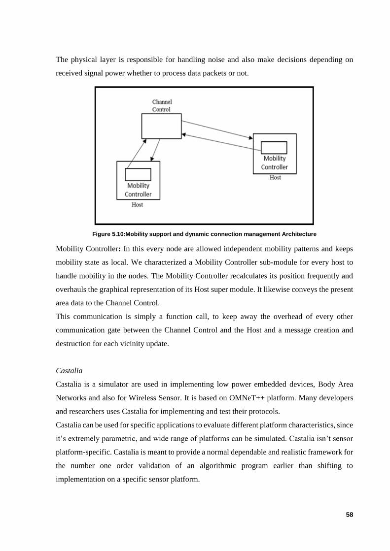
58
The physical layer is responsible for handling noise and also make decisions depending on
received signal power whether to process data packets or not.
Figure 5.10:Mobility support and dynamic connection management Architecture
Mobility Controller: In this every node are allowed independent mobility patterns and keeps
mobility state as local. We characterized a Mobility Controller sub-module for every host to
handle mobility in the nodes. The Mobility Controller recalculates its position frequently and
overhauls the graphical representation of its Host super module. It likewise conveys the present
area data to the Channel Control.
This communication is simply a function call, to keep away the overhead of every other
communication gate between the Channel Control and the Host and a message creation and
destruction for each vicinity update.
Castalia
Castalia is a simulator are used in implementing low power embedded devices, Body Area
Networks and also for Wireless Sensor. It is based on OMNeT++ platform. Many developers
and researchers uses Castalia for implementing and test their protocols.
Castalia can be used for specific applications to evaluate different platform characteristics, since
it’s extremely parametric, and wide range of platforms can be simulated. Castalia isn’t sensor
platform-specific. Castalia is meant to provide a normal dependable and realistic framework for
the number one order validation of an algorithmic program earlier than shifting to
implementation on a specific sensor platform.

59
Test code compiled for a specific sensor node platform is not useful in Castalia. For this type
of situations there are other available simulators/emulators.
The main features of Castalia are:
Empirically measured data is used in defining Advanced channel model
A map of path loss defined by Model, not merely connections between nodes
Temporal variation of path loss is in Complex model
Mobility of the nodes are fully supported
With the received signal strength. Interference is handled, not as separate feature
Individual node variations allowed with multiple TX power levels
Flexible carrier sensing and physical process model
Extended sensing modelling provisions
CPU power consumption, Node clock drift
Routing and MAC protocols
Designed for expansion and adaptation
5.4 Node Controller
In the wireless sensor network are 3 kinds of sensor nodes: the conventional nodes are
responsible for collecting information or sensed knowledge. Sensor nodes have a resource
constraint. This is the main reason for sensor node not able to store large amount of data with
it. Sensor nodes acts as gateway nodes for connecting source and destination or to the external
entities called observers. Node is also responsible for data processing. Observer could be
implemented in node. Similarly, actuators can also be delivered to actuate or control on a
monitored area in Wireless sensor networks.
Node Architecture
The components of sensor node and its structure is shown in Figure 5.11. The architecture of a
well-known wireless sensor nodes includes 4 subsystems. A computing subsystem such as a
ALU, microprocessor and memory, a communication subsystem including a short range radio
for wireless communication, sensing subsystem that links the node to the physical world and
includes a set of sensors and actuators, and a power supply subsystem, which homes the battery
and the (optionally available) DC-DC converter, and powers the relaxation of the node. Every
subsystem plays a chief role in the sensor node.

60
Figure 5.11:Senor Node Architecture
Radio: It permits wireless communication among sensing nodes and also the outside
world. Generally, it operates in unlicensed band 2.4 GHz and with low data rate with
single channel. For green energy intake, it operates in four unique modes: Transmit,
receive, Idle and Standby modes.
Microprocessor: It gives intelligence to the sensor node. The microprocessor controls
the sensors, executes conversation protocols and signal processing algorithms at the
gathered sensor information. To conserve strength, microprocessor works in four
exclusive modes: off, sleep, idle, and energetic. In sleep mode, the CPU and maximum
inner peripherals are became off, and may solely be activated by an external event
(interrupt). In idle mode, the central processing unit is still inactive, however different
peripherals are active. In the energetic states, the CPU and all peripherals are active.
Sensor: It interprets physical phenomena to electric signals. There exists an expansion
of sensors that measure environmental parameters inclusive of sound, image,
temperature, intensity, magnetic fields, temperature and many others. Because of the
diversity of sensors, there's no general power intake figure. To reduce energy intake,
low energy components can be used on the cost of performance that is not required.

61
Battery: The battery is a vital element in sensor node. It provides power to all or any
component of sensing element nodes. Consequently, sensor node period wholly depends
upon on battery and network’s lifetime relies upon at the lifetime of sensing nodes. The
amount of power drained from a battery must be checked. Therefore, energy
consumption is an important issue to prolong the sensing element nodes lifetime.
Node Modules
In node module, the conventional layers according to the IP model can be found, the physical
layer, the network layer, the application layer and the MAC layer. The physical layer takes care
regrading receiving, the collision handling and also the adjacent layers are connected with many
pairs of OMNeT++ “gates”. The first pair is used for sending and receiving messages with
respective to environment, which includes control message for nodes. In second pair exchange
control messages between the layers and support control communication are used.
Examples are the request from the MAC layer to a physical layer is to perform carrier
anticipation, or the indication of the physical layer to the MAC layer that the transmission of
the complete message is finished. Figure 5.12, shows in Network Interface Card (NIC) both
physical and MAC layer are grouped into it for other communication techniques.
Figure 5.12:Node and NIC structure

62
In MiXiM, as a laptop with exceptional NICs, similarly like GSM, Bluetooth and IEEE 802.11
may be modelled. The mobility module is accountable for the mobility of a node or an object.
Battery module is used for power related issues. The Address Resolution Protocol are handled
by Arp modules for the exchange among MAC and network addresses. The utility module is
derived from the blackboard module added in the Mobility Framework. It accommodates
critical assignments which can be subdivided into two: Firstly, it gives a general interface for
collecting analytical data of a simulation. Using the utility module for collecting information
statistically which have minimal impact on the performance of the simulation and leaves full
freedom for several analysis methods. Secondly, the utility module keeps parameters that want
to be achieved with multiple module within a node. One example is the environment in a node,
which is determined and up to date by the mobility module, but additionally required with the
physical layer and possibly the local module.
Timer
MiXiM provides a variety of timer modules to be utilized by protocols, allowing easy use of
timers without having total understanding about the system, and presents normal common
functionality for the creation and destruction of timers with least user intervention. MiXiM has
three types of timers:
Simple one-shot Timer, when it is started it sends once n seconds,
Repeat Timer, is similar to simple one-shot timer in this sends every n seconds each,
Frame Timer, that similar to the Repeat Timer, all the conventional separate timers for
exclusive nodes are authorised to send regarding the same time. Additionally, with
OMNeT++ objects can be “attached” to timers to permit for storing arbitrary timer-
associated data.
Mobility module and Connection Management
The movement of node or other elements is done by mobility in each entity. With interval
parameter accuracy of the mobility can be adjusted. The BaseMobility composition will be
liable for the graphical representation. On every occasion the location is modified, it updates
the graphical representation. One of the modules that desires the information about changes in
the position of a node is the physical layer which is responsible for updating the placement with
the ConnectionManager.

63
Connection Management
For authorizing connections between nodes and also terminate connection whenever distance
between them exceeds, these are the roles by ConnectionManager. The loss of connectivity can
be because to the motion (i.e. the nodes move too much apart) or due to a modification in
transmission power or a crashed node, so forth. The very critical instance influencing the
maximal interference distance is then attenuation due to the objects inward to the line-of-sight
for the two vital nodes. Each object has a frequency dependent on the actual attenuating
instances. All objects ought to archive with the Object Manager. The extra attenuation is then
determined through including up the frequency based attenuation factor of the objects
intersecting the line. The connection manager can use these values for adjusting the maximal
interference distance of the two nodes and the presence of the objects will cause two nodes to
be disconnected.
5.5 Implementation
Server to node
The following code shows, the communication of server to node messages in the network.
These messages are represented by type 1 in the code.
//Server to node communication
if(msgtyp == 1){
sendData.clear();
sendData.push_back(1);
sendData.push_back(energy);
sendData.push_back(recvMsg->getData(2)-1);
sendData.push_back( recvMsg->getData(3) );
progress["deltaMsgs"] = recvMsg->getData(3);
if(progress["repropagate"] && !(myNetwAddr == progress["serverid"])){
createMsg(myNetwAddr,myNetwAddr,"neighbour response");
progress["sendmsgcnt"]=0;
}
progress["repropagate"] = 0;
//receiving node
if(recvMsg->getData(2) >= myPreferenceModel[recvMsg->getSrcid()].grad){
myPreferenceModel[recvMsg->getSrcid()].grad = recvMsg->getData(2);
myPreferenceModel[recvMsg->getSrcid()].gradsrc = recvMsg->getSrcid();
}
if(recvMsg->getData(2)>= myPreferenceModel[progress["serverid"]].grad){
myPreferenceModel[progress["serverid"]].grad = recvMsg->getData(2);
myPreferenceModel[progress["serverid"]].gradsrc = recvMsg->getSrcid();
}
myPreferenceModel[recvMsg->getSrcid()].pref = recvMsg->getData(1);
}

64
Node to server
The given below code an implementation of node to server message communication and these
messages are represented by type 3 messages in code.
if(msgtyp == 3 && myNetwAddr == recvMsg->getDestid()){
if( !(progress["serverid"] == myNetwAddr) ){
//msg to server
sendData.clear();
sendData.push_back(3);
sendData.push_back(100);
//get node to forward
int curSelectNeighbourEnergy=
myPreferenceModel[progress["serverid"]].pref;
//if for current node observation that other node has more energy use
other node (implicit weight bei value dif)
int maxenergy = curSelectNeighbourEnergy;
//in case of source == destination init with 0
if(recvMsg->getSrcid() ==
myPreferenceModel[progress["serverid"]].gradsrc)
maxenergy = 0;
int maxidx = myPreferenceModel[progress["serverid"]].gradsrc;
if(energyobserve)
for(std::map<int,PreferenceModelElement>::iterator it =
myPreferenceModel.begin(); it!= myPreferenceModel.end(); it++){
if(myPreferenceModel[it->first].pref >
maxenergy+progress["eswitchweight"]
&& it->first != recvMsg->getSrcid() && it->first !=
myNetwAddr && it->first != progress["serverid"]){
maxenergy = myPreferenceModel[it->first].pref;
maxidx = it->first;
}
}
if(energy > 0 && !temporalconnectionoff){
energy--;
createMsg(myNetwAddr, maxidx,"msg to server");
}
Node unavailability
In the following code node 0 is made offline for a certain period of time to know how the
network is balanced. Whenever there are changes in the network topology

65
case TICEVENT:
myEnergyVector.record(energy);
ticMsg = new cMessage("timer", TICEVENT);
scheduleAt(simTime()+1, ticMsg);
progress["repropagate"] = 1;
if(simTime() == 120 &&
FindModule<AiSNetworkLayer*>::findSubModule(getModuleByPath("AiSNetwork.N
ode[0]"))->myNetwAddr == myNetwAddr){
temporalconnectionoff = 1;
}
if(simTime() == 154 &&
FindModule<AiSNetworkLayer*>::findSubModule(getModuleByPath("AiSNetwork.N
ode[0]"))->myNetwAddr == myNetwAddr){
temporalconnectionoff = 0;
}
Rule 2 implementation
The following code shows the implementation of rule 2, where deltamsgs are being checked
for choosing strategies of routing in the network.
if( (observeaccept ==1) && (progress["deltaMsgs"] <
progress["sendmsgcnt"]/2) ){
// stategies-set contains: deltamsg(infoofserverreceivedmsgs)/sendmsgcnt,
parameters eswitchweight,// strategy-generating module:energy other path
compared to best energy path
char bubblestring[60];
sprintf(bubblestring, "adaptRateDeliver d>5=%i, also if
de<10",progress["newRecMsgs"]-progress["oldRecMsgs"]);
getParentModule()->bubble(bubblestring);
ev << bubblestring;
//energy -> shortest path
if(myPreferenceModel[progress["serverid"]].gradsrc != maxidx){
maxidx = myPreferenceModel[progress["serverid"]].gradsrc;
step = 1; //sp
}
else{
// shortest path -> energy
maxidx = energyStrategy(maxenergy,1);
step = 2; //sp other option
}
}
Rule 3 implementation for light detection
The following code shows the implementation of rule 3, after implementing rule 2 an additional
light event is observer for detection.

66
if(msgtyp == 4){
//if we are destination stop
if(recvMsg->getDestid() == myNetwAddr){
char bubblestring[60];
sprintf(bubblestring, "light message stop received");
getParentModule()->bubble(bubblestring);
ev << bubblestring;
lighttoobserver = 0; //resolved point in time
sprintf(bubblestring, "switch of notify light");
getParentModule()->bubble(bubblestring);
delete msg;
return;
}

67
6 Results and Analysis
In chapter we see the results obtained from complete thesis work and analysing the obtained
results in more detailed. The given below screenshot is a simulation environment implemented
with five sensor nodes with one sensor node sending messages to the server throughout the
network using proposed routing protocol
6.1 Experimental Setup
In this experimental setup five nodes are used in which node 3 is sending messages to the server
throughout the simulation process. Node 3, is vertex having two neighbour’s node 0 and node
4. Routing of messages are done through either node 0 to server or through node 4. This
simulation network is fixed type and connection manager is responsible for forming links
among nodes.
Figure 6.1:Simulation environment in OMNeT++

68
6.2 Implementated routing protocols on simulation environment
6.2.1 Shortest Path Routing
With the same simulation network, shortest path routing is implemented. In which node
responds with respectively. For shortest path, it considers the number of hops to reach the
destination (server). In our case node 3 is transmitting messages to the server. Therefore, in
order to achieve the shortest path to server, messages are routed through node 0, because it has
very less hop count to reach server than other alternative routes in the network.
Figure 6.2:Graph of shortest path routing implementation
From the above graph, we can observe the energy levels of the various nodes in the simulation
network. As in our case node 3 (which is represented by the colour yellow) is sending messages
to server and node 3 energy is slowly degrading. Initially node 3 has 200 as energy by the end
of the time period 110 it is approx.95. We can witness as there is no messages transmitted
further (time approx. 110) because node 0 which is having an energy of 100 at the start of the
simulation is totally exhausted. Therefore, by the principle of shortest path (observing hop
count) no further messages are sent to the server.

69
6.2.2 Energy based path routing
In energy based routing, in order to transfer messages to the destination. The energies of the all
its neighbouring nodes are considered. For example, one is trying to send messages to the
destination. First, it considers energy level/value of its neighbours if one of its neighbour having
high energy value when compared to others, the message is transmitted through that node. Here,
we defined energy switch, which decides the threshold limit in order to route messages. For an
instance if threshold limit is 20, that means sending node compares its neighbours if their
difference is less than 20 it follows the shortest path else if threshold limit 20 is crossed it
switches to possible energy path to reach the destination.
Figure 6.3:Graph showing results of implementing energy based routing
From the above figure 6.3, illustrates the graph of energy levels of various sensing nodes and
messages received at the server with respectively. As node 3 is represented with the yellow line,
and messages received with the red line. Here we can see that energies of the other sensing
nodes are also used.
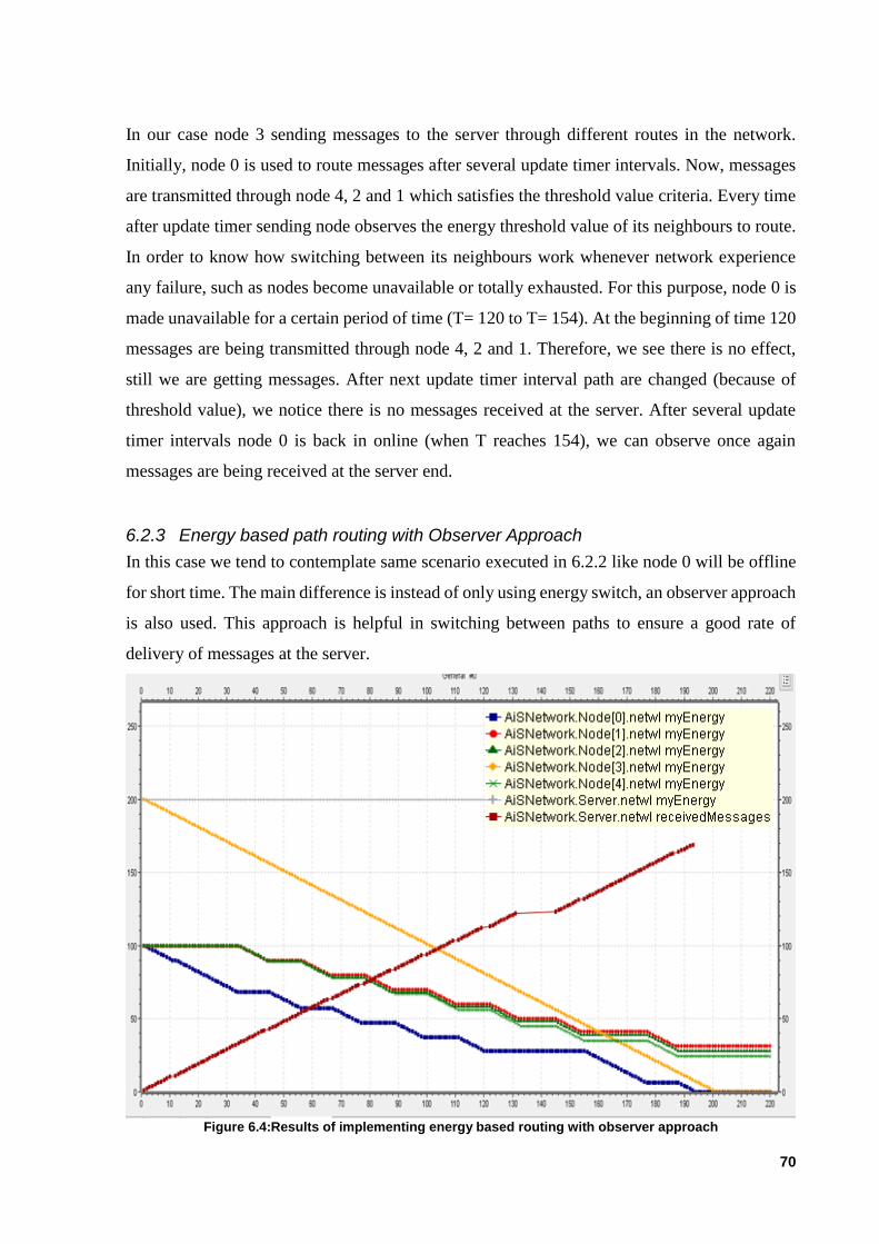
70
In our case node 3 sending messages to the server through different routes in the network.
Initially, node 0 is used to route messages after several update timer intervals. Now, messages
are transmitted through node 4, 2 and 1 which satisfies the threshold value criteria. Every time
after update timer sending node observes the energy threshold value of its neighbours to route.
In order to know how switching between its neighbours work whenever network experience
any failure, such as nodes become unavailable or totally exhausted. For this purpose, node 0 is
made unavailable for a certain period of time (T= 120 to T= 154). At the beginning of time 120
messages are being transmitted through node 4, 2 and 1. Therefore, we see there is no effect,
still we are getting messages. After next update timer interval path are changed (because of
threshold value), we notice there is no messages received at the server. After several update
timer intervals node 0 is back in online (when T reaches 154), we can observe once again
messages are being received at the server end.
6.2.3 Energy based path routing with Observer Approach
In this case we tend to contemplate same scenario executed in 6.2.2 like node 0 will be offline
for short time. The main difference is instead of only using energy switch, an observer approach
is also used. This approach is helpful in switching between paths to ensure a good rate of
delivery of messages at the server.
Figure 6.4:Results of implementing energy based routing with observer approach

71
During our case study, when node 0 is unavailable for one update interval, sending node
changes its routing strategy by switching paths (energy to shortest or shortest to energy). So,
that the network can experience less or avoid message loss. From figure 6.4, the graph shows
that there has been improvement in the rate of delivery of the message when using this approach.
Comparison of both routing technique approaches
Below figure 6.5, depicts a graph shows both the techniques in one graph, as we can notice that
both are having similar energy usage in normal scenario where every node is active (that is up
to T=130), thereafter special case is considered to replicate the real system scenario into
simulation making one node unavailable for a certain amount of time (node 0).
Figure 6.5:Results of both routing schemes in one graph
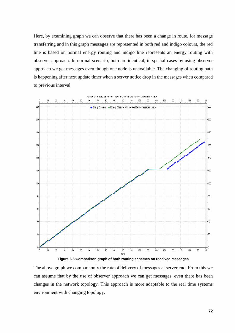
72
Here, by examining graph we can observe that there has been a change in route, for message
transferring and in this graph messages are represented in both red and indigo colours, the red
line is based on normal energy routing and indigo line represents an energy routing with
observer approach. In normal scenario, both are identical, in special cases by using observer
approach we get messages even though one node is unavailable. The changing of routing path
is happening after next update timer when a server notice drop in the messages when compared
to previous interval.
Figure 6.6:Comparison graph of both routing schemes on received messages
The above graph we compare only the rate of delivery of messages at server end. From this we
can assume that by the use of observer approach we can get messages, even there has been
changes in the network topology. This approach is more adaptable to the real time systems
environment with changing topology.

73
6.2.4 Rule 3 Implementation
Figure 6.7:Rule 3 implementation

74
From figure 6.7, show how messages are exchanged between the server and event sensing node.
In (a) whenever an event occurs sensing node alerts the server with the light message. In our
case node2 is used to trigger light event which is than observed by the camera connected to the
server, when the server gets light message it responds to this message by controlling process
chain in our industrial scenario. From (b) after receiving light message from one of its sensing
node. Now, the server sends response message to notify node 2, as acknowledgment to event
triggered node, that it has received its message. In this setup notify node 2 message is
broadcasted on the network. From (c) node 2 receives notify message from server. Now, node
2 will switch off the light source. Therefore, energy of the light source can be saved. Whenever
any sensing node triggers an event than light message is send to server.
This rule can be implemented in various event sensing situations such as: pressure, humidity,
sound detection and water level can be used based on the application.

75
Summary
The thesis was started with the goal to provide an efficient solution for the wireless sensor
network energy consumption. The research was carried out, comparing the different
possibilities to solve the problem. There are many approaches proposed by researchers in this
field of optimize usage of network energy. The thesis aim was also to use sensing nodes energy
efficiently to make network work for longer duration of time. For this a general routing
techniques are used to create a new approach. This approach is more adaptive and proves to be
more efficient.
In the present thesis work, an observer is introduced for observing messages received at the
server. Which determines the rate of delivery, the most challenging part of the thesis was an
observer weight switch, this helps in switching between routing paths when certain condition
is satisfied. There was challenge in deciding switch weight value, switch weight value should
be determined by the size of the network topology. Inappropriate switch weight leads to extent
usage of energy of nodes. This leads network unbalanced and not further operation. The
challenge was to learn that in a short time and apply to the thesis implementation to get the
required results. C++ with OMNeT++ library for implementing layers, and for achieving
wireless properties MiXiM is used along OMNeT++. There were also tough times during the
work, with MiXiM framework on OMNeT++. As a plan to create new a routing technique two
routing schemes were considered to implement an observer approach on wireless sensor
network those are shortest path and gradient based energy path. Observer component defines
switch weight to decide when to switch routes. For industrial purpose another rule is introduced
for real time sensing scenarios. The results show how efficient it is than other conventional
routing techniques.

76
Future Scope
In this section, a list of task or activities are discussed which can be applied in future on the
proposed method to solve some problems and other kind of improvements. The following things
are:
• Timing organization: it is required in every wireless sensor network, which has many
sensing nodes for sending critical data to the base station or server. This organization is
helpful whenever several node wants to send data at the same time, there must be some
kind of synchronization between sending nodes. Can be done giving priority to
particular nodes or nodes nearer to the destination will take the priority of sending data.
• Energy weight update latency: in case of messages over the node is bigger than usual,
then the network should use a bigger energy switch to stay longer in balancing mode.
This will ensure good network operation without loss in information sending to server.
By appropriate, energy weight update latency network lifetime can be improved.
• Retransmission: by sending data again into the network, nodes energy is wasted because
of loss of data while transmitting to low connectivity nodes to pass the data on. This can
be checked by how strong the signal received during a neighbour’s response stage.
• Prioritizing: prioritizing messages from sensing nodes for more critical messages to be
further processed first.
• Mobility: in this thesis, work is done on a fixed network with all sensing nodes are fixed
in the area. Implementing in mobile network can be done where all nodes are moving
and nodes are added or removed from the network based on their connectivity.
• Clustering: this thesis further developed for cluster based sensor networks, where
clustering can be done based on the energy level of the nodes in a cluster to form cluster
head to transmit messages to the server.

77
Content of Compact Disk
ObserverApproach: This folder contains the complete implementation codes in the form of a
zip file which can be directly imported to the OMNeT++ simulation software. This zip file
consists of several folders including results, xml file and source code also. The source code will
be available in ‘src’ folder. It contains implemented code on various layers such as, network,
MAC, application layers and with package explained in chapter 5. Result folder contains
screenshots of the results obtained on the implemented simulation network.
Note: this project is developed in OMNeT++ and uses MiXiM framework for mobility.
Documents: This folder contains the following items:
•User Guide: For brief understanding about OMNeT++ and explains project creation.
•MiXiM: This document explains the overview of MiXiM framework working with OMNeT++
on implementing wireless and mobile networks.
•FinalThesisreport: This pdf contains a soft copy of Thesis report.

78
Bibliography
1 A. Köpke, M. S. (2008). Simulating Wireless and Mobile Networks in OMNeT++ The MiXiM
Vision. ACM 978-963-9799-20-2.
2 András Varga, R. H. (March, 2008). AN OVERVIEW OF THE OMNeT++ SIMULATION
ENVIRONMENT. Marseille, France: International Standard Book Number.
3 Bhushan N. Mahajan, D. V. (2010). Dynamic Route and Threshold Level Selection in Energy
Efficient WSN . Third International Conference on Emerging Trends in Engineering and
Technology. IEEE.
4 C. Mallanda, A. S. (Jan 2005). Simulating Wireless Sensor Networks with OMNeT++. NSF-
ITR, IIS-0312632.
5 Chunyao FU, Z. J. (January 2013). An Energy Balanced Algorithm of LEACH Protocol in
WSN. IJCSI International Journal of Computer Science.
6 Curt Schurgers, M. B. (2001). Energy Efficient Routing In Wireless Sensor Networks. IEEE, 5.
7 Datta, M. R. An Energy–Efficient Routing Technique for Privacy Preservation of Assets
Monitored with WSN. Proceeding of the 2014 IEEE Students' Technology Symposium.
8 Dhannendra Singh, S. S. (2014). Energy Efficient Source Based Tree Routing With Time Stamp
in WSN . IEEE.
9 Dinu Gopal, D. S. (20 15). Performance Evaluation Of Hybrid Energy Efficient Cluster Based
Routing Scheme For Mobile Sink Based Wsn . IEEE .
10 Ernesto García Davis, A. C. (2013). Improving Packet Delivery Performance of
Publish/Subscribe Protocols in Wireless Sensor Networks. Sensors ISSN 1424-8220.
11 Fateh, M. O. (2015). Simulation, Comparison and Analysis of Wireless Sensor Networks
Protocols: LEACH, LEACH-C, LEACH-1R, and HEED. IEEE, 5.
12 Feng Chen, F. D. A Simulation Model of IEEE 802.15.4 in OMNeT++. 91058 Erlangen,
Germany: Computer Networks and Communication Systems University of Erlangen-
Nuremberg.
13 G.Lakshmi Phani, K. S. (2010). ERFLA: Energy Efficient Combined Routing, Fusion,
Localization Algorithm in Cognitive WSN . IEEE.
14 Gupta, D. K. (2013). A Review on Wireless Sensor Networks. Inter national Conference on
Recent Trends in Applied Sciences with Engineering Applications.
15 Haafizah Rameeza Shaukat, F. H. (2014). MWSN Modeling Using OMNeT++ Simulator. IEEE
Fifth International Conference on Intelligent Systems, Modelling and Simulation, 6.
16 Hammerseth, S. (November 29, 2011). Implementing RPL in a mobile and fixed wireless sensor
network with OMNeT++. Oslo, Norway: University Of Oslo, Department of Informatics.

79
17 Heena Dhawan, S. W. (June 2014). A Comparative Study on LEACH Routing Protocol and its
Variants in Wireless Sensor Networks: A Survey. International Journal of Computer
Applications (0975 – 8887), Volume 95– No.8.
18 Humber, G. (Juni 2009). Quality of Information Aware Data Delivery in Wireless Sensor
Networks. Department of Information Technology Uppsala University.
19 Jabed Faruque, A. H. Gradient-Based Routing in Sensor Networks. Los Angeles, CA 90089,
USA: Department of Computer Engineering University of Southern California.
20 Kamal, J. N.-K. Routing Techniques in Wireless Sensor Networks: A Survey. Ames, Iowa
50011: Dept. of Electrical and Computer Engineering Iowa State University,.
21 Karl Wessel, M. S. (March 2009). MiXiM – The Physical Layer An Architecture Overview.
International workshop on OMNeT++, (S. 8). Rome,Italy.
22 Koksal, M. M. (October 22, 2008). A Survey of Network Simulators Supporting Wireless
Networks. Ankara, TURKEY: Department of Computer Science, Middle East Technical
University.
23 Lusheng Miao, K. D. (July 2016). Energy-Efficient Algorithm Based on Gradient Based Routing
in Wireless Sensor Networks. Pretoria South Africa: French South African Institute of
Technology (F’SATI), Tshwane University of Technology,.
24 Mariusz Gł ˛abowski, B. M. (2013). Efficiency Evaluation of Shortest Path Algorithms. The
Ninth Advanced International Conference on Telecommunications.
25 ME Migaboa, K. D. (2015). Gradient-Based Routing for Energy Consumption Balance in
Multiple Sinks-based Wireless Sensor Networks. The Seventh International Symposium on
Applications of Ad hoc and Sensor Networks (AASNET’15).
26 Mohammad Masumuzzaman Bhuiyan, I. G. (2011 ). CODAR: Congestion and Delay Aware
Routing to Detect Time Critical Events in WSNs. IEEE.
27 Poonam Lohan, R. C. (2012). Geography-Informed Sleep Scheduled and Chaining Based
Energy Efficient Data Routing in WSN. IEEE Students’ Conference on Electrical, Electronics
and Computer Science.
28 Ritwik Banerjee, C. K. (2014 ). Energy Efficient Routing and Bypassing Energy-Hole through
Mobile Sink in WSN . IEEE.
29 S Taruna, M. R. (April 2013). EVENT DRIVEN ROUTING PROTOCOLS FOR WIRELESS
SENSOR NETWORK- A SURVEY. International Journal on Computational Sciences &
Applications.
30 Samira Yessad, N. T. (2012). Balanced Energy Efficient Routing Protocol for WSN. The 2nd
International Conference on Communications and Information Technology (ICCIT):
Communication Networks and Systems, Hammamet. IEEE.
31 Sankarasubramaniam, O. B. Event-to-Sink Reliable Transport in Wireless Sensor Networks.
IEEE/ACM Transactions On Networking.

80
32 Sarma, R. K. (2013). Energy Efficient Routing Protocols for WSN's. International Conference
on Computer Communication and Informatics. Coimbatore, INDIA: IEEE.
33 Sohail Jabbar, A. E. (Feb 2016). Threshold Based Load Balancing Protocol for Energy Efficient
Routing in WSN. ISBN 978-89-5519-155-4.
34 Team, O. D. (2014). OMNeT++ User Guide. András Varga and OpenSim Ltd.
35 Wang Daoyuan, T. H. (2007). Energy-Efficient Routing Research for WSN. Beijing: IEEE.
36 Witold Drytkiewicz, S. S. (January 22, 2003). A Mobility Framework for OMNeT++.
Berlin,Germany.: Telecommunication Networks Group.
37 Xia Li, W. G. (2013). An energy-efficient routing protocol based on particle swarm clustering
algorithm and inter-cluster routing algorithm for WSN . IEEE.
38 Xiaodong Xian, W. S. (2008). Comparison of OMNET++ and Other Simulator for WSN
Simulation. IEEE.
39 Younis, K. A.. A Survey on Routing Protocols for Wireless Sensor Networks. Baltimore County,
Baltimore, MD 21250: Department of Computer Science and Electrical Engineering, University
of Maryland .