Balancing of Masseslecture - 1 Balancing of Masses Theory of Machine 4 b) When the plane of the...
47
lecture - 1 Balancing of Masses Theory of Machine 1 Balancing of Masses A car assembly line. In this chapter we shall discuss the balancing of unbalanced forces caused by rotating masses, in order to minimize the loads on bearings and stresses in the various members, which causes dangerous vibrations when a machine is running. The following cases are important from the subject point of view: 1. Balancing of a single rotating mass by a single mass rotating in the same plane. 2. Balancing of a single rotating mass by two masses rotating in different planes. 3. Balancing of different masses rotating in the same plane. 4. Balancing of different masses rotating in different planes. 1. Balancing of a Single Rotating Mass By a Single Mass Rotating in the Same Plane Consider a disturbing mass m 1 attached to a shaft rotating at ω rad/s as shown in Fig .1. Let r 1 be the radius of rotation of the mass m 1 . We know that the centrifugal force exerted by the mass m 1 on the shaft, F Cl = m 1 . ω 2 . r 1 …………….(1)
Transcript of Balancing of Masseslecture - 1 Balancing of Masses Theory of Machine 4 b) When the plane of the...
lecture - 1 Balancing of Masses Theory of Machine
1
Balancing of Masses
A car assembly line.
In this chapter we shall discuss the balancing of unbalanced forces caused by
rotating masses, in order to minimize the loads on bearings and stresses in the
various members, which causes dangerous vibrations when a machine is running.
The following cases are important from the subject point of view:
1. Balancing of a single rotating mass by a single mass rotating in the same plane.
2. Balancing of a single rotating mass by two masses rotating in different planes.
3. Balancing of different masses rotating in the same plane.
4. Balancing of different masses rotating in different planes.
1. Balancing of a Single Rotating Mass By a Single Mass Rotatingin the Same Plane
Consider a disturbing mass m1 attached to a shaft rotating at ω rad/s as shown in
Fig .1. Let r1 be the radius of rotation of the mass m1. We know that the centrifugal
force exerted by the mass m1 on the shaft,
FCl = m1. ω2. r1 …………….(1)
lecture - 1 Balancing of Masses Theory of Machine
2
Fig. 1. Balancing of a single rotating mass by a single mass rotating in the same plane.
This centrifugal force produces bending moment on the shaft. In order to
counteract the effect of this force, a balancing mass (m2) may be attached in the
same plane of rotation as that of disturbing mass (m1) such that the centrifugal
forces due to the two masses are equal and opposite.
Let r2 = Radius of rotation of the balancing mass m2, centrifugal force dueto mass m2,
FC2 = m2. ω2. r2 …………….(2)
Equating equations (1) and (2),
m1. ω2. r1 = m2. ω2. r2 or m1. r1 = m2. r2
2. Balancing of a Single Rotating Mass By Two Masses Rotating inDifferent Planes
In order to put the system in complete balance, two balancing masses are placed in
two different planes, parallel to the plane of rotation of the disturbing mass, There
are two possibilities may arise while attaching the two balancing masses:
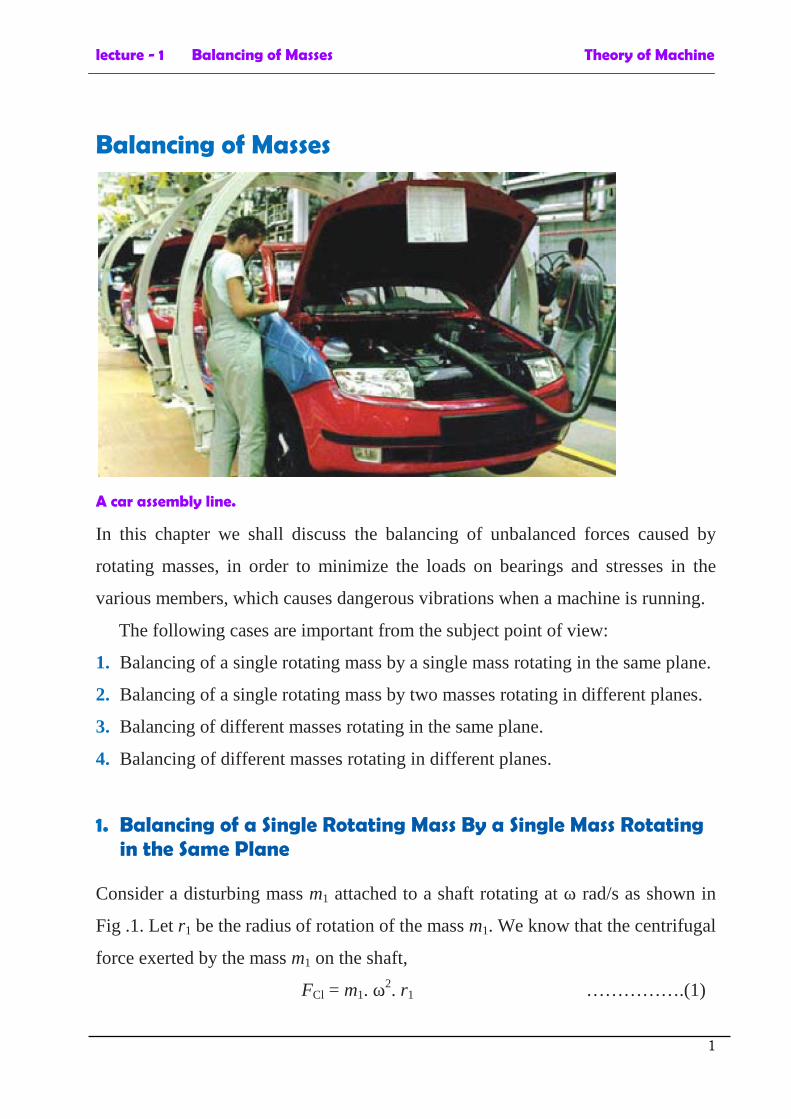
a) When the plane of the disturbing mass lies in between the planes ofthe two balancing masses
Consider a disturbing mass m balanced by two rotating masses m1 and m2 as
shown in Fig. 2. Let r, r1 and r2 be the radii of rotation of the masses m, m1 and
m2 respectively.
lecture - 1 Balancing of Masses Theory of Machine
3
Fig .2. Balancing of a single rotating mass by two rotating masses in different planes when theplane of single rotating mass lies in between the planes of two balancing masses.
The net force acting on the shaft must be equal to zero
FC = FCl + FC2
FC : Centrifugal force exerted by the mass m
FC1 : Centrifugal force exerted by the mass m1
FC2 : Centrifugal force exerted by the mass m2
m. ω2. r = m1. ω2. r1 + m2. ω2. r2
m. r = m1. r1 + m2. r2
Now in order to find the magnitude of balancing force at the bearing B of a
shaft, take moments about A. Therefore
FC1 × l = FC × l2 or m1. ω2. r1 × l = m. ω2. r × l2
m1. r1 × l = m. r × l2
Similarly, in order to find the balancing force at the bearing A of a shaft, take
moments about B. Therefore
FC2 × l = FC × l1 or m2. ω2. r2 × l = m. ω2. r × l1
m2. r2 × l = m. r × l1
lecture - 1 Balancing of Masses Theory of Machine
4
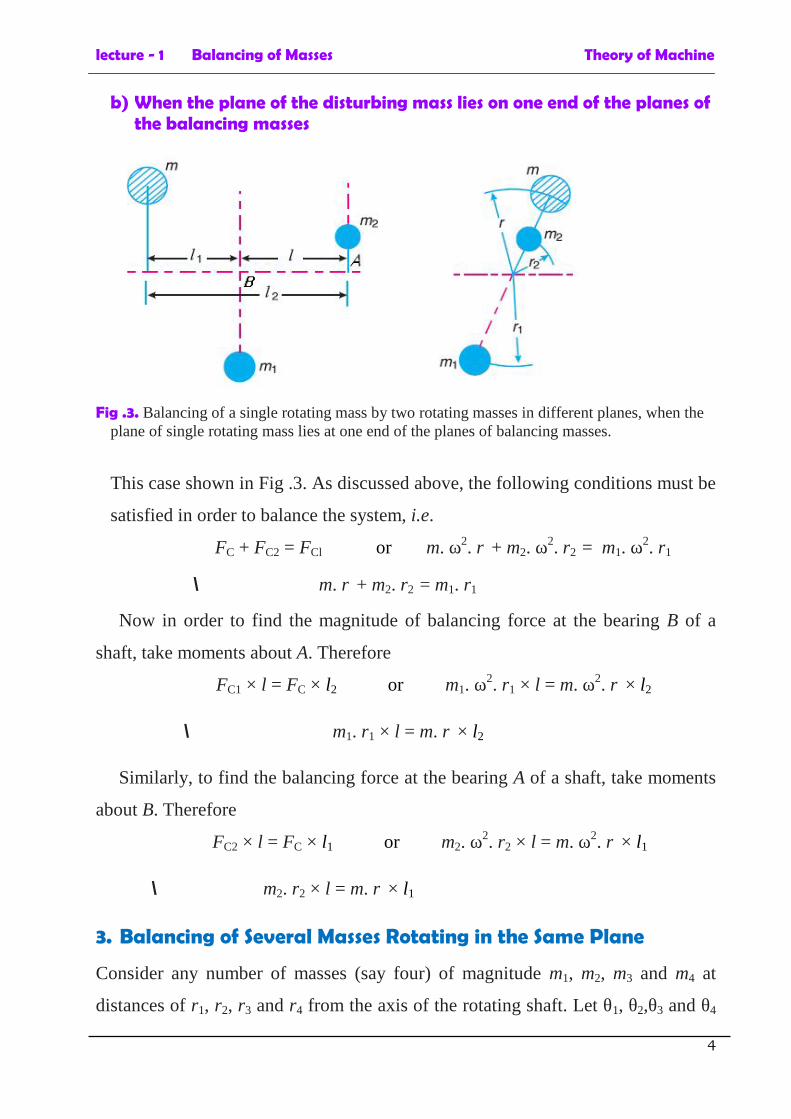
b) When the plane of the disturbing mass lies on one end of the planes ofthe balancing masses
Fig .3. Balancing of a single rotating mass by two rotating masses in different planes, when theplane of single rotating mass lies at one end of the planes of balancing masses.
This case shown in Fig .3. As discussed above, the following conditions must be
satisfied in order to balance the system, i.e.
FC + FC2 = FCl or m. ω2. r + m2. ω2. r2 = m1. ω2. r1
m. r + m2. r2 = m1. r1
Now in order to find the magnitude of balancing force at the bearing B of a
shaft, take moments about A. Therefore
FC1 × l = FC × l2 or m1. ω2. r1 × l = m. ω2. r × l2
m1. r1 × l = m. r × l2
Similarly, to find the balancing force at the bearing A of a shaft, take moments
about B. Therefore
FC2 × l = FC × l1 or m2. ω2. r2 × l = m. ω2. r × l1
m2. r2 × l = m. r × l1
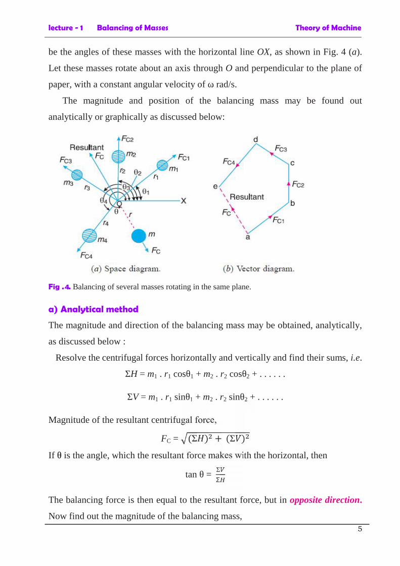
3. Balancing of Several Masses Rotating in the Same Plane
Consider any number of masses (say four) of magnitude m1, m2, m3 and m4 at
distances of r1, r2, r3 and r4 from the axis of the rotating shaft. Let θ1, θ2,θ3 and θ4
lecture - 1 Balancing of Masses Theory of Machine
5
be the angles of these masses with the horizontal line OX, as shown in Fig. 4 (a).
Let these masses rotate about an axis through O and perpendicular to the plane of
paper, with a constant angular velocity of ω rad/s.
The magnitude and position of the balancing mass may be found out
analytically or graphically as discussed below:
Fig .4. Balancing of several masses rotating in the same plane.
a) Analytical method
The magnitude and direction of the balancing mass may be obtained, analytically,
as discussed below :
Resolve the centrifugal forces horizontally and vertically and find their sums, i.e.
ΣH = m1 . r1 cosθ1 + m2 . r2 cosθ2 + . . . . . .
ΣV = m1 . r1 sinθ1 + m2 . r2 sinθ2 + . . . . . .
Magnitude of the resultant centrifugal force,
FC = (Σ ) + (Σ )If θ is the angle, which the resultant force makes with the horizontal, then
tan θ = Σ
The balancing force is then equal to the resultant force, but in opposite direction.
Now find out the magnitude of the balancing mass,
lecture - 1 Balancing of Masses Theory of Machine
6
FC = m. r
where m = Balancing mass, and
r = Its radius of rotation.
b) Graphical method
The magnitude and position of the balancing mass may also be obtained
graphically using Table: 1 and then draw:
1. Find the centrifugal force (or product of the mass and radius of rotation)
exerted by each mass on the rotating shaft.
2. Draw the vector diagram with the obtained centrifugal forces to some suitable
scale.
3. The closing side of polygon ae represents the resultant force in magnitude and
direction, as shown in Fig. 4 (b).
4. The balancing force is, then, equal to the resultant force, but in opposite
direction.
5. Find the magnitude of the balancing mass (m) at a given radius of rotation (r),
m.r = Resultant of m1.r1, m2.r2, m3.r3 and m4.r4
Table: 1
No. ofmasses Mass (m) Radius (r) Angle()
Centrifugal force 2
(m.r)
1 m1 r1 1 m1 r1
2 m2 r2 2 m2.r2
3 m3 r3 3 m3.r3
4 m4 r4 4 m4.r4
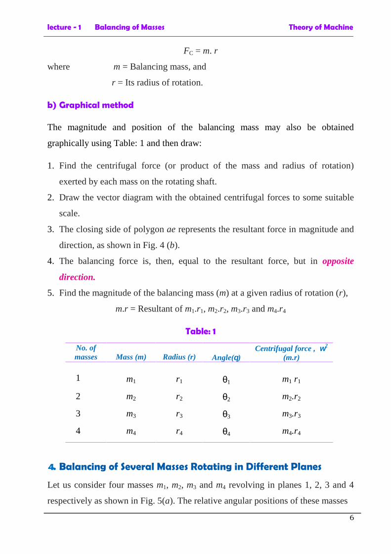
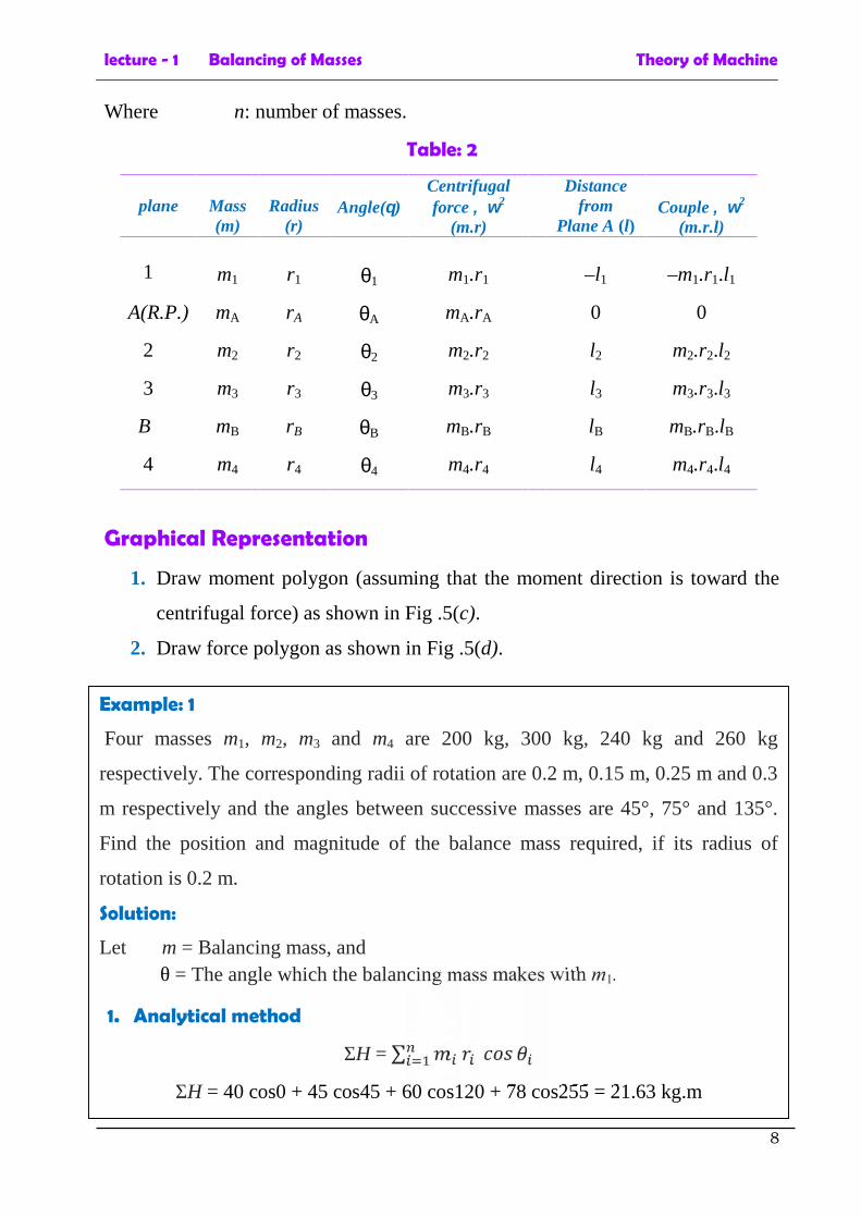
4. Balancing of Several Masses Rotating in Different Planes
Let us consider four masses m1, m2, m3 and m4 revolving in planes 1, 2, 3 and 4
respectively as shown in Fig. 5(a). The relative angular positions of these masses
lecture - 1 Balancing of Masses Theory of Machine
7
Fig. 5. Balancing of several masses rotating in different planes.
are shown in Fig. 5(b). The magnitude of the balancing masses mA and mB in
planes A and B may be obtained as discussed below:
1. Take one of the planes, say A as the reference plane (R.P.).
2. Tabulate the data as shown in Table: 2.
3. The couples about the reference plane must balance, i.e. the resultant couple
must be zero. ∑ + mB rB lB cos = 0∑ sin + mB rB lB sin = 0
4. The forces in the reference plane must balance, i.e. the resultant force must
be zero. ∑ + mA rA cos = 0∑ sin + mA rA sin = 0
lecture - 1 Balancing of Masses Theory of Machine
8
Where n: number of masses.
Table: 2
plane Mass(m)
Radius(r)
Angle()Centrifugalforce 2
(m.r)
Distancefrom
Plane A (l)Couple 2
(m.r.l)
1 m1 r1 1 m1.r1 –l1 –m1.r1.l1
A(R.P.) mA rA A mA.rA 0 0
2 m2 r2 2 m2.r2 l2 m2.r2.l2
3 m3 r3 3 m3.r3 l3 m3.r3.l3
B mB rB B mB.rB lB mB.rB.lB
4 m4 r4 4 m4.r4 l4 m4.r4.l4
Graphical Representation
1. Draw moment polygon (assuming that the moment direction is toward the
centrifugal force) as shown in Fig .5(c).
2. Draw force polygon as shown in Fig .5(d).
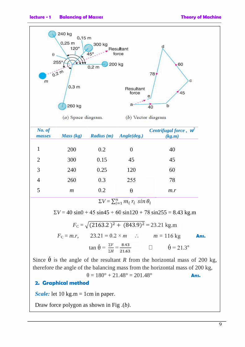
Example: 1
Four masses m1, m2, m3 and m4 are 200 kg, 300 kg, 240 kg and 260 kg
respectively. The corresponding radii of rotation are 0.2 m, 0.15 m, 0.25 m and 0.3
m respectively and the angles between successive masses are 45°, 75° and 135°.
Find the position and magnitude of the balance mass required, if its radius of
rotation is 0.2 m.
Solution:
Let m = Balancing mass, andθ = The angle which the balancing mass makes with m1.
1. Analytical method
ΣH = ∑ΣH = 40 cos0 + 45 cos45 + 60 cos120 + 78 cos255 = 21.63 kg.m
lecture - 1 Balancing of Masses Theory of Machine
9
No. ofmasses Mass (kg) Radius (m) Angle(deg.)
Centrifugal force 2
(kg.m)
1 200 0.2 0 40
2 300 0.15 45 45
3 240 0.25 120 60
4 260 0.3 255 78
5 m 0.2 m.r
ΣV = ∑ΣV = 40 sin0 + 45 sin45 + 60 sin120 + 78 sin255 = 8.43 kg.m
FC = (2163.2 ) + (843.9) = 23.21 kg.m
FC = m.r, 23.21 = 0.2 × m m = 116 kg Ans.
tan θ =Σ
=.. = 21.3
Since θ is the angle of the resultant R from the horizontal mass of 200 kg,therefore the angle of the balancing mass from the horizontal mass of 200 kg,
θ = 180° + 21.48° = 201.48° Ans.
2. Graphical method
Scale: let 10 kg.m = 1cm in paper.
Draw force polygon as shown in Fig .(b).
lecture - 1 Balancing of Masses Theory of Machine
10
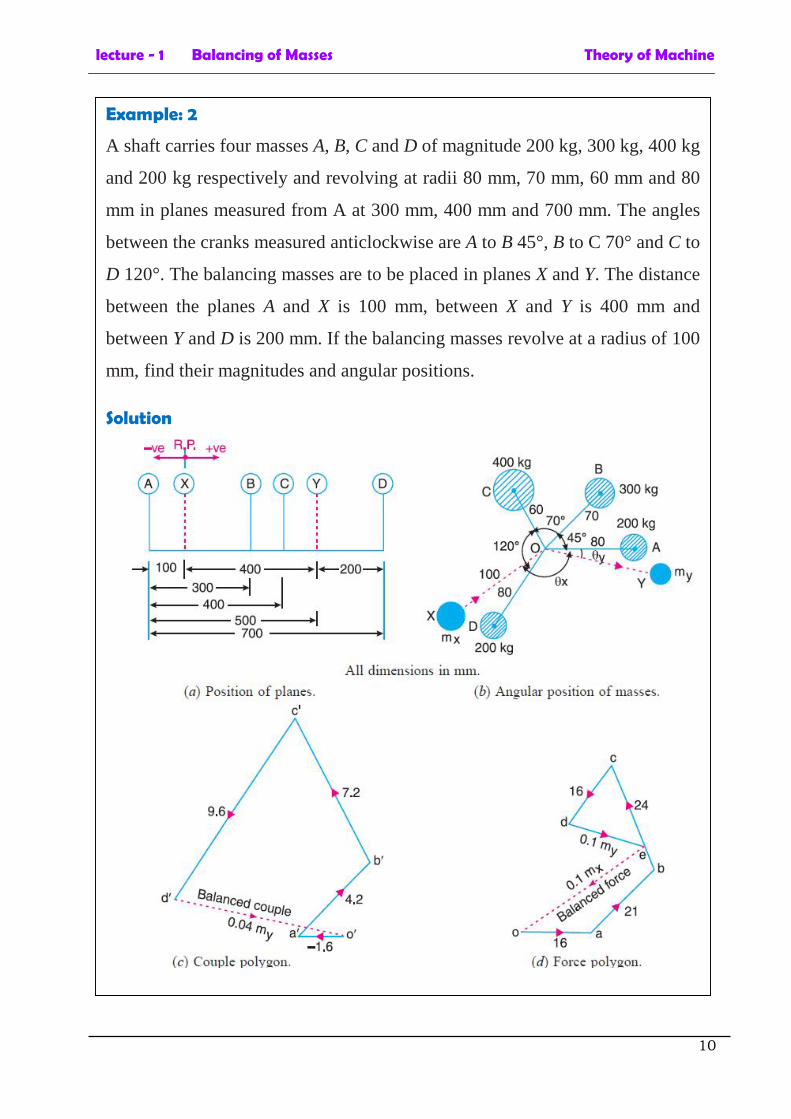
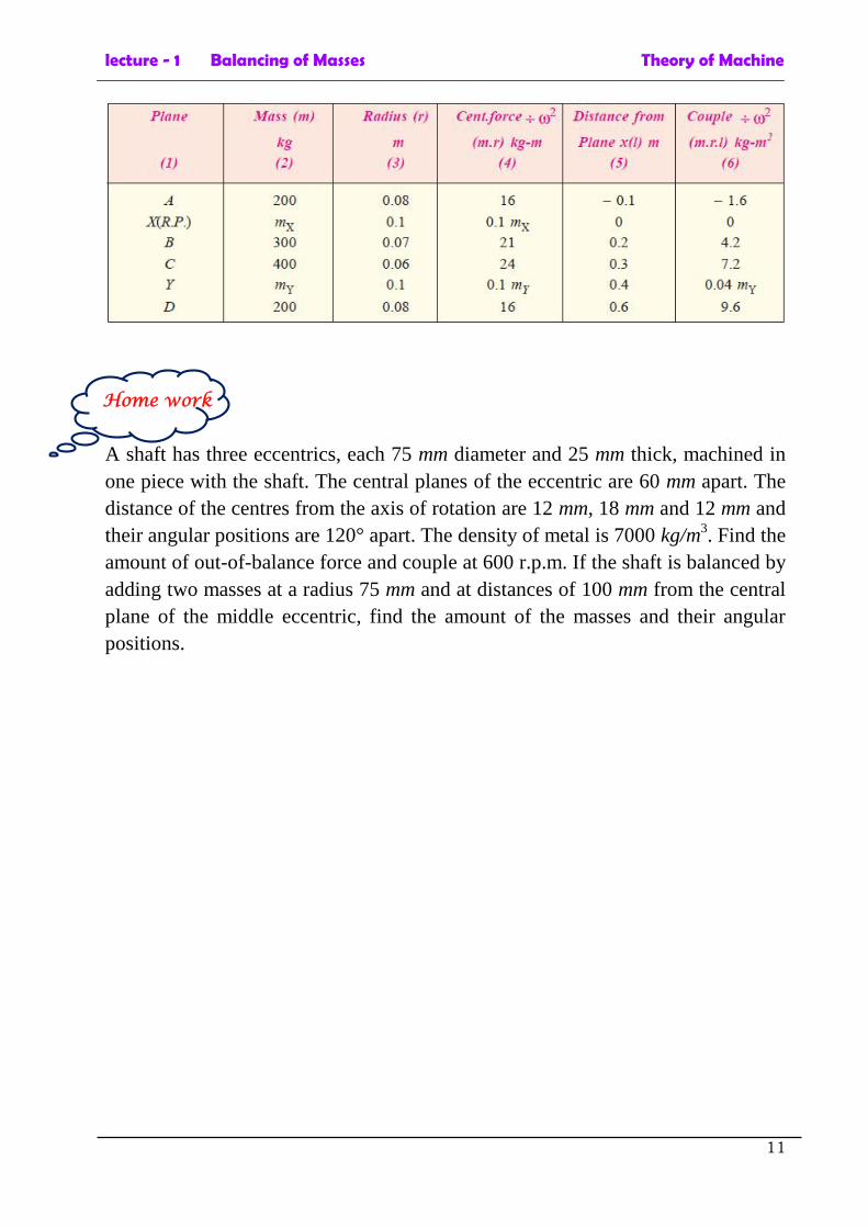
Example: 2
A shaft carries four masses A, B, C and D of magnitude 200 kg, 300 kg, 400 kg
and 200 kg respectively and revolving at radii 80 mm, 70 mm, 60 mm and 80
mm in planes measured from A at 300 mm, 400 mm and 700 mm. The angles
between the cranks measured anticlockwise are A to B 45°, B to C 70° and C to
D 120°. The balancing masses are to be placed in planes X and Y. The distance
between the planes A and X is 100 mm, between X and Y is 400 mm and
between Y and D is 200 mm. If the balancing masses revolve at a radius of 100
mm, find their magnitudes and angular positions.
Solution
lecture - 1 Balancing of Masses Theory of Machine
11
A shaft has three eccentrics, each 75 mm diameter and 25 mm thick, machined inone piece with the shaft. The central planes of the eccentric are 60 mm apart. Thedistance of the centres from the axis of rotation are 12 mm, 18 mm and 12 mm andtheir angular positions are 120° apart. The density of metal is 7000 kg/m3. Find theamount of out-of-balance force and couple at 600 r.p.m. If the shaft is balanced byadding two masses at a radius 75 mm and at distances of 100 mm from the centralplane of the middle eccentric, find the amount of the masses and their angularpositions.
Home work
lecture - 1 Balancing of Masses Theory of Machine
12
Solution:
lecture - 1 Balancing of Masses Theory of Machine
13
lecture - 2 Cams Theory of Machine
1
Cams
A cam is a rotating machine element which gives
reciprocating or oscillating motion to another
element known as follower. The cam and follower
is one of the simplest as well as one of the most
important mechanisms found in modern machinery today. The cams are widely
used for operating the inlet and exhaust valves of internal combustion engines.
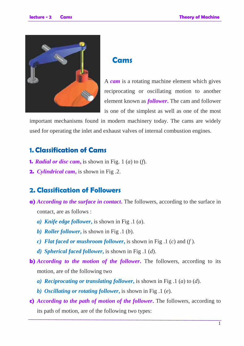
1. Classification of Cams
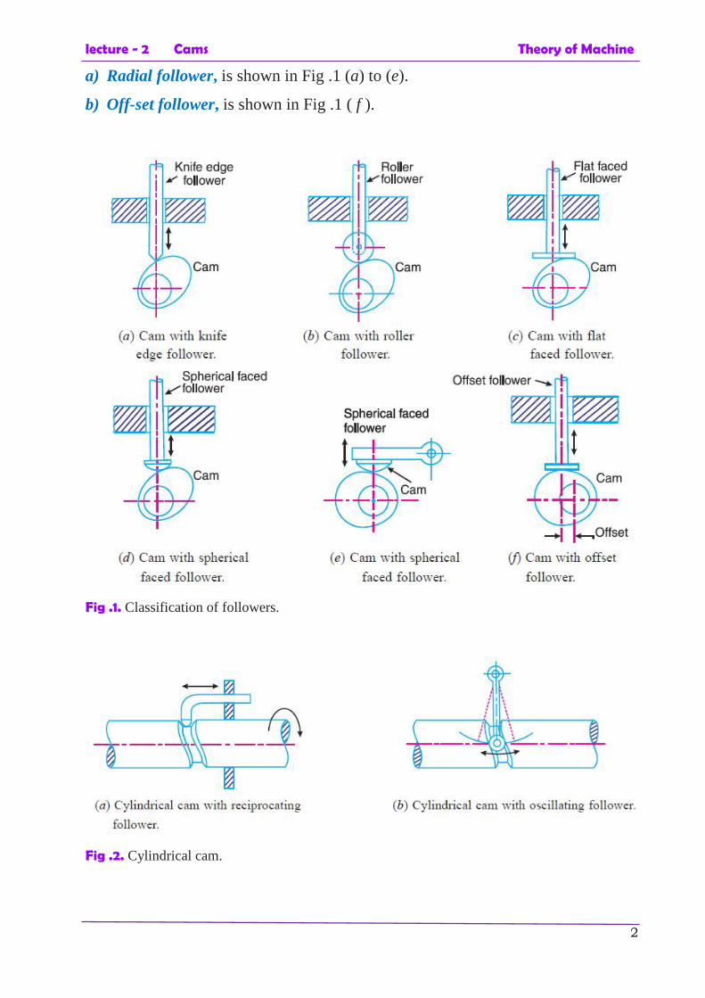
1. Radial or disc cam, is shown in Fig. 1 (a) to (f).
2. Cylindrical cam, is shown in Fig .2.
2. Classification of Followers
a) According to the surface in contact. The followers, according to the surface in
contact, are as follows :
a) Knife edge follower, is shown in Fig .1 (a).
b) Roller follower, is shown in Fig .1 (b).
c) Flat faced or mushroom follower, is shown in Fig .1 (c) and (f ).
d) Spherical faced follower, is shown in Fig .1 (d).
b) According to the motion of the follower. The followers, according to its
motion, are of the following two
a) Reciprocating or translating follower, is shown in Fig .1 (a) to (d).
b) Oscillating or rotating follower, is shown in Fig .1 (e).
c) According to the path of motion of the follower. The followers, according to
its path of motion, are of the following two types:
lecture - 2 Cams Theory of Machine
2
a) Radial follower, is shown in Fig .1 (a) to (e).
b) Off-set follower, is shown in Fig .1 ( f ).
Fig .1. Classification of followers.
Fig .2. Cylindrical cam.
lecture - 2 Cams Theory of Machine
3
3. Motion of the Follower
The follower, during its travel, may have one of the following motions.
1. Uniform velocity,
2. Simple harmonic motion, and
3. Uniform acceleration and retardation.
We shall now discuss the displacement, velocity and acceleration diagrams for
the cam when the follower moves with the above mentioned motions.
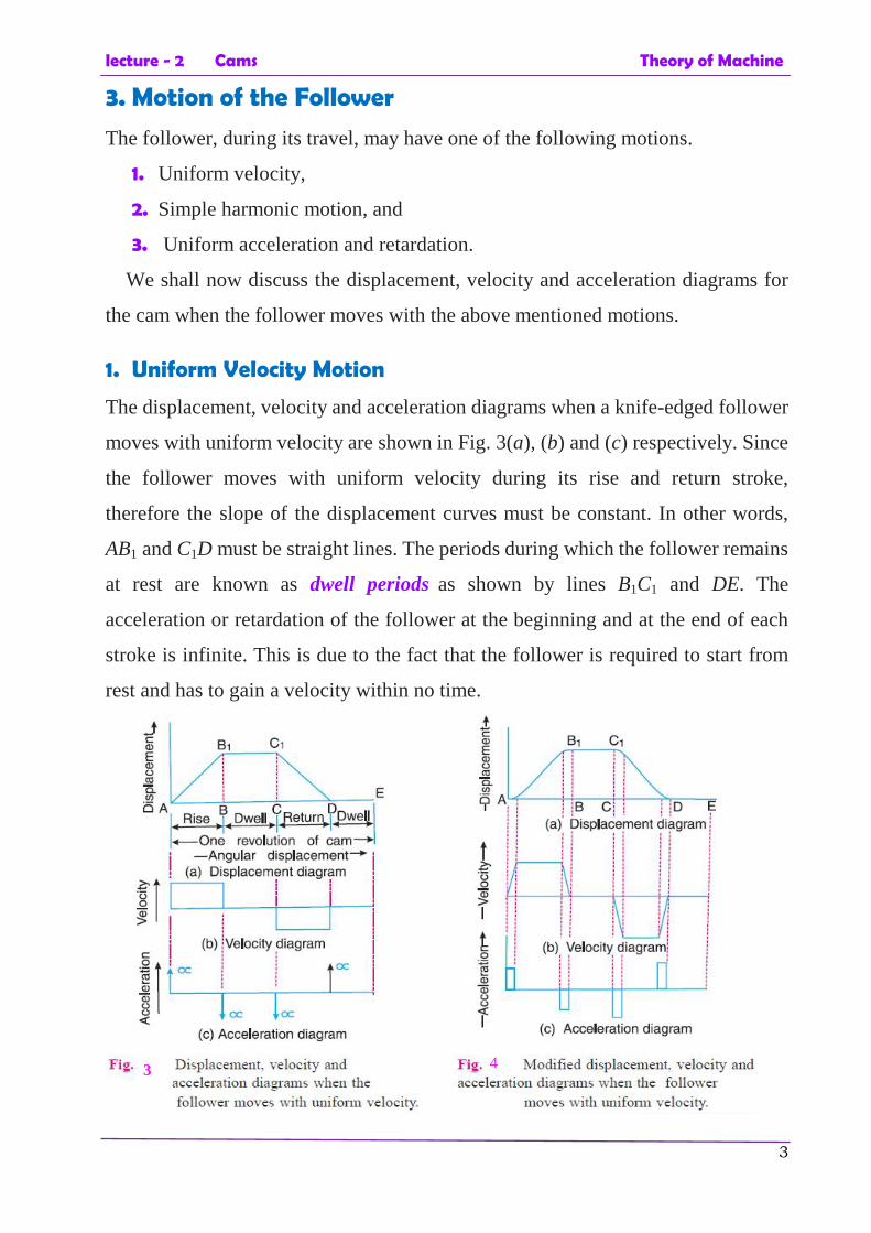
1. Uniform Velocity Motion
The displacement, velocity and acceleration diagrams when a knife-edged follower
moves with uniform velocity are shown in Fig. 3(a), (b) and (c) respectively. Since
the follower moves with uniform velocity during its rise and return stroke,
therefore the slope of the displacement curves must be constant. In other words,
AB1 and C1D must be straight lines. The periods during which the follower remains
at rest are known as dwell periods as shown by lines B1C1 and DE. The
acceleration or retardation of the follower at the beginning and at the end of each
stroke is infinite. This is due to the fact that the follower is required to start from
rest and has to gain a velocity within no time.
3 4
lecture - 2 Cams Theory of Machine
4
In order to have the acceleration and retardation within the finite limits, it is
necessary to modify the conditions which govern the motion of the follower. This
may be done by rounding off the sharp corners of the displacement diagram at the
beginning and at the end of each stroke, as shown in Fig. 4(a). By doing so, the
velocity of the follower increases gradually to its maximum value at the beginning
of each stroke and decreases gradually to zero at the end of each stroke as shown
in Fig. 4(b).
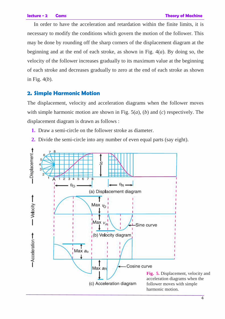
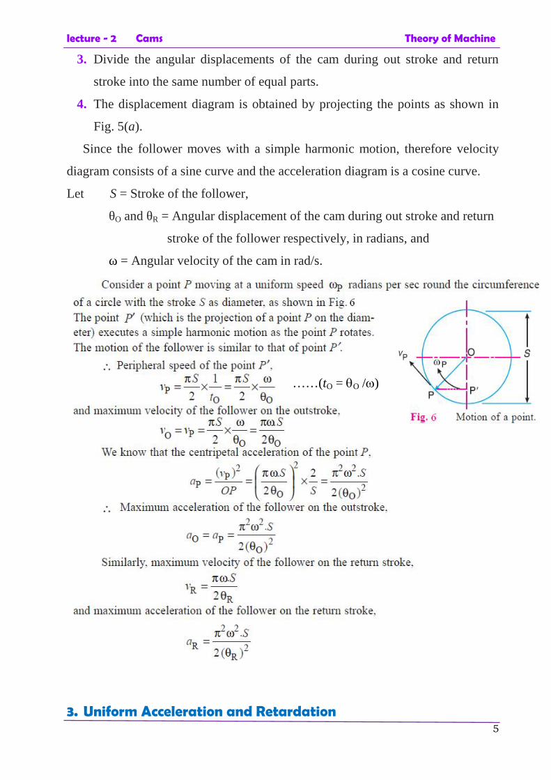
2. Simple Harmonic Motion
The displacement, velocity and acceleration diagrams when the follower moves
with simple harmonic motion are shown in Fig. 5(a), (b) and (c) respectively. The
displacement diagram is drawn as follows :
1. Draw a semi-circle on the follower stroke as diameter.
2. Divide the semi-circle into any number of even equal parts (say eight).
Fig. 5. Displacement, velocity andacceleration diagrams when thefollower moves with simpleharmonic motion.
lecture - 2 Cams Theory of Machine
5
3. Divide the angular displacements of the cam during out stroke and return
stroke into the same number of equal parts.
4. The displacement diagram is obtained by projecting the points as shown in
Fig. 5(a).
Since the follower moves with a simple harmonic motion, therefore velocity
diagram consists of a sine curve and the acceleration diagram is a cosine curve.
Let S = Stroke of the follower,
θO and θR = Angular displacement of the cam during out stroke and return
stroke of the follower respectively, in radians, and
ω = Angular velocity of the cam in rad/s.
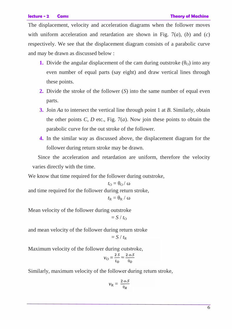
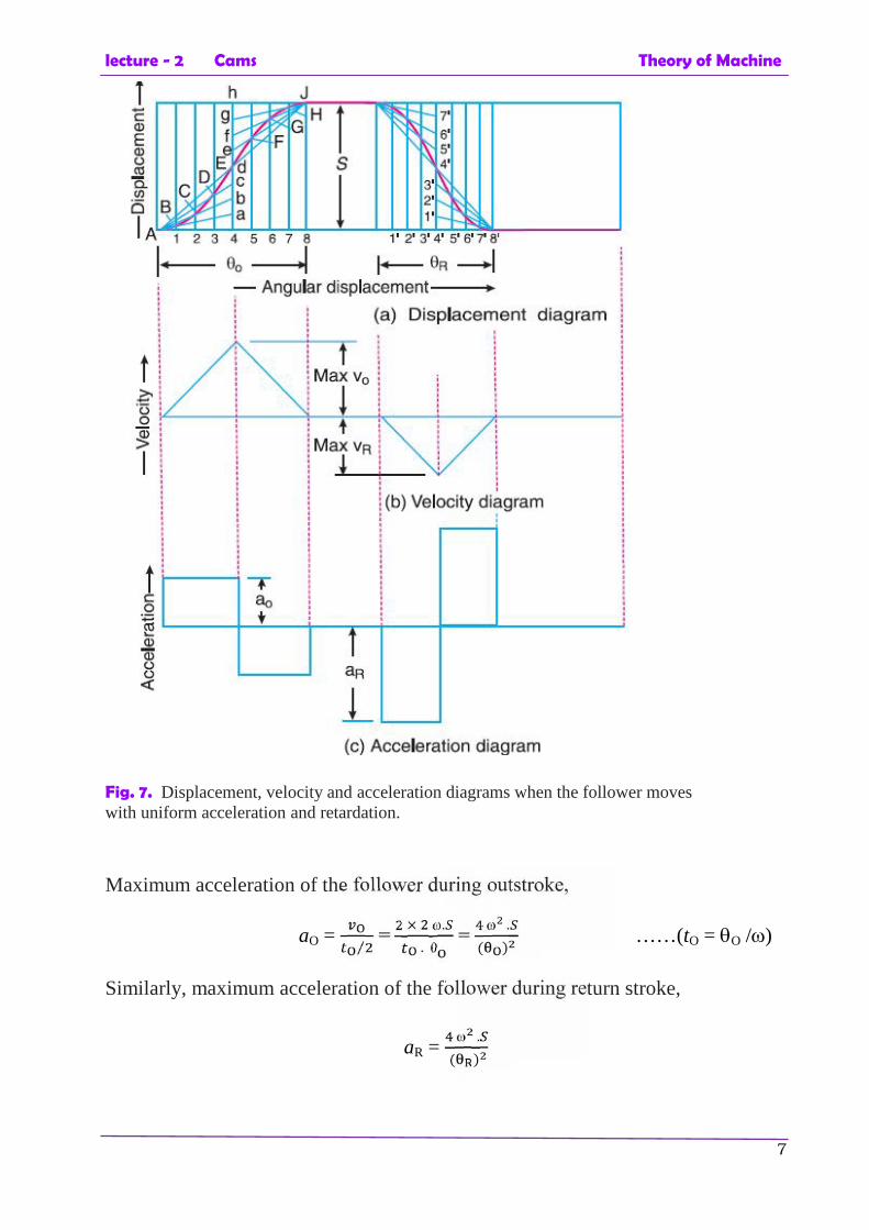
3. Uniform Acceleration and Retardation
……(tO = O /)
lecture - 2 Cams Theory of Machine
6
The displacement, velocity and acceleration diagrams when the follower moves
with uniform acceleration and retardation are shown in Fig. 7(a), (b) and (c)
respectively. We see that the displacement diagram consists of a parabolic curve
and may be drawn as discussed below :
1. Divide the angular displacement of the cam during outstroke (θO) into any
even number of equal parts (say eight) and draw vertical lines through
these points.
2. Divide the stroke of the follower (S) into the same number of equal even
parts.
3. Join Aa to intersect the vertical line through point 1 at B. Similarly, obtain
the other points C, D etc., Fig. 7(a). Now join these points to obtain the
parabolic curve for the out stroke of the follower.
4. In the similar way as discussed above, the displacement diagram for the
follower during return stroke may be drawn.
Since the acceleration and retardation are uniform, therefore the velocity
varies directly with the time.
We know that time required for the follower during outstroke,tO = θO / ω
and time required for the follower during return stroke,tR = θR / ω
Mean velocity of the follower during outstroke= S / tO
and mean velocity of the follower during return stroke= S / tR
Maximum velocity of the follower during outstroke,
vO = =.θ
Similarly, maximum velocity of the follower during return stroke,
vR =.θ
lecture - 2 Cams Theory of Machine
7
Fig. 7. Displacement, velocity and acceleration diagrams when the follower moveswith uniform acceleration and retardation.
Maximum acceleration of the follower during outstroke,
aO = ⁄ =× .. θ
= .( ) ……(tO = O /)
Similarly, maximum acceleration of the follower during return stroke,
aR = .( )
lecture - 2 Cams Theory of Machine
8
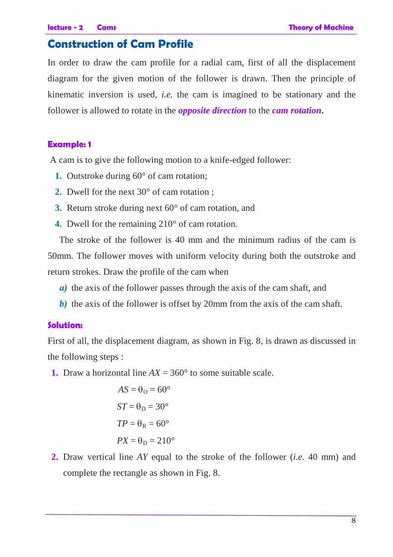
Construction of Cam Profile
In order to draw the cam profile for a radial cam, first of all the displacement
diagram for the given motion of the follower is drawn. Then the principle of
kinematic inversion is used, i.e. the cam is imagined to be stationary and the
follower is allowed to rotate in the opposite direction to the cam rotation.
Example: 1
A cam is to give the following motion to a knife-edged follower:
1. Outstroke during 60° of cam rotation;
2. Dwell for the next 30° of cam rotation ;
3. Return stroke during next 60° of cam rotation, and
4. Dwell for the remaining 210° of cam rotation.
The stroke of the follower is 40 mm and the minimum radius of the cam is
50mm. The follower moves with uniform velocity during both the outstroke and
return strokes. Draw the profile of the cam when
a) the axis of the follower passes through the axis of the cam shaft, and
b) the axis of the follower is offset by 20mm from the axis of the cam shaft.
Solution:
First of all, the displacement diagram, as shown in Fig. 8, is drawn as discussed in
the following steps :
1. Draw a horizontal line AX = 360° to some suitable scale.
AS = O = 60°
ST = D = 30°
TP = R = 60°
PX = D = 210°
2. Draw vertical line AY equal to the stroke of the follower (i.e. 40 mm) and
complete the rectangle as shown in Fig. 8.
lecture - 2 Cams Theory of Machine
9
3. Divide the angular displacement during outstroke and return stroke into any
equal number of even parts (say six) and draw vertical lines through each
point.
4. Since the follower moves with uniform velocity during outstroke and return
stroke, therefore the displacement diagram consists of straight lines. Join AG
and HP.
5. The complete displacement diagram is shown by AGHPX.
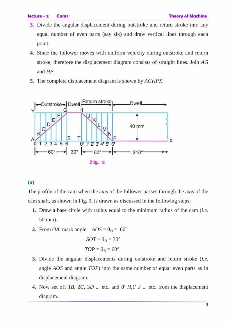
(a)
The profile of the cam when the axis of the follower passes through the axis of the
cam shaft, as shown in Fig. 9, is drawn as discussed in the following steps:
1. Draw a base circle with radius equal to the minimum radius of the cam (i.e.
50 mm).
2. From OA, mark angle AOS = O = 60°
SOT = D = 30°
TOP = R = 60°
3. Divide the angular displacements during outstroke and return stroke (i.e.
angle AOS and angle TOP) into the same number of equal even parts as in
displacement diagram.
4. Now set off 1B, 2C, 3D ... etc. and 0′ H,1′ J ... etc. from the displacement
diagram.
lecture - 2 Cams Theory of Machine
10
5. Join the points A, B, C,... M, N, P with a smooth curve. The curve AGHPA is
the complete profile of the cam.
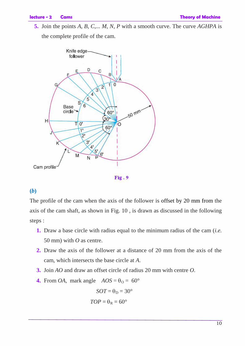
(b)
The profile of the cam when the axis of the follower is offset by 20 mm from the
axis of the cam shaft, as shown in Fig. 10 , is drawn as discussed in the following
steps :
1. Draw a base circle with radius equal to the minimum radius of the cam (i.e.
50 mm) with O as centre.
2. Draw the axis of the follower at a distance of 20 mm from the axis of the
cam, which intersects the base circle at A.
3. Join AO and draw an offset circle of radius 20 mm with centre O.
4. From OA, mark angle AOS = O = 60°
SOT = D = 30°
TOP = R = 60°
lecture - 2 Cams Theory of Machine
11
5. Divide the angular displacement during outstroke and return stroke (i.e.
angle AOS and angle TOP) into the same number of equal even parts as in
displacement diagram.
6. Now from the points 1, 2, 3 ... etc. and 0′,1′, 2′,3′ ... etc. on the base circle,
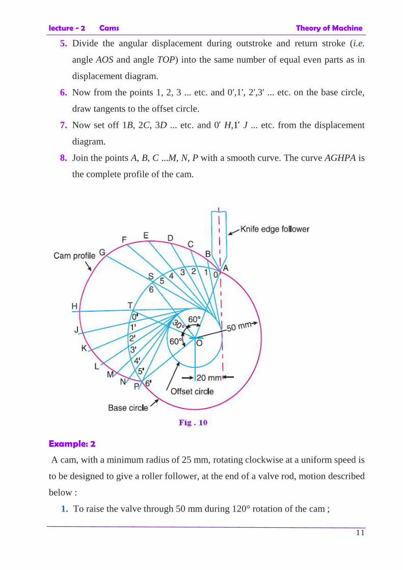
draw tangents to the offset circle.
7. Now set off 1B, 2C, 3D ... etc. and 0′ H,1′ J ... etc. from the displacement
diagram.
8. Join the points A, B, C ...M, N, P with a smooth curve. The curve AGHPA is
the complete profile of the cam.
Example: 2
A cam, with a minimum radius of 25 mm, rotating clockwise at a uniform speed is
to be designed to give a roller follower, at the end of a valve rod, motion described
below :
1. To raise the valve through 50 mm during 120° rotation of the cam ;
lecture - 2 Cams Theory of Machine
12
2. To keep the valve fully raised through next 30°;
3. To lower the valve during next 60°; and
4. To keep the valve closed during rest of the revolution i.e. 150° ;
The diameter of the roller is 20 mm and the diameter of the cam shaft is 25 mm.
Draw the profile of the cam when
a) the line of stroke of the valve rod passes through the axis of the cam shaft,
b) the line of the stroke is offset 15 mm from the axis of the cam shaft.
The displacement of the valve, while being raised and lowered, is to take place
with simple harmonic motion. Determine the maximum acceleration of the valve
rod when the cam shaft rotates at 100 r.p.m.
Draw the displacement, the velocity and the acceleration diagrams for one
complete revolution of the cam.
Solution:
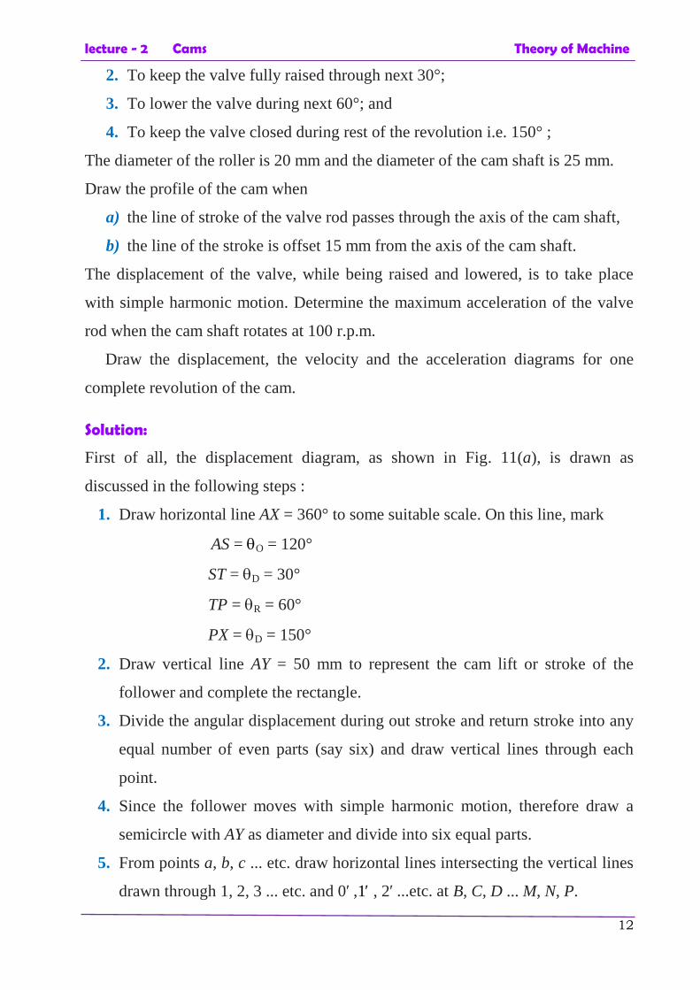
First of all, the displacement diagram, as shown in Fig. 11(a), is drawn as
discussed in the following steps :
1. Draw horizontal line AX = 360° to some suitable scale. On this line, mark
AS = O = 120°
ST = D = 30°
TP = R = 60°
PX = D = 150°
2. Draw vertical line AY = 50 mm to represent the cam lift or stroke of the
follower and complete the rectangle.
3. Divide the angular displacement during out stroke and return stroke into any
equal number of even parts (say six) and draw vertical lines through each
point.
4. Since the follower moves with simple harmonic motion, therefore draw a
semicircle with AY as diameter and divide into six equal parts.
5. From points a, b, c ... etc. draw horizontal lines intersecting the vertical lines
drawn through 1, 2, 3 ... etc. and 0′ ,1′ , 2′ ...etc. at B, C, D ... M, N, P.
lecture - 2 Cams Theory of Machine
13
6. Join the points A, B, C ... etc. with a smooth curve.
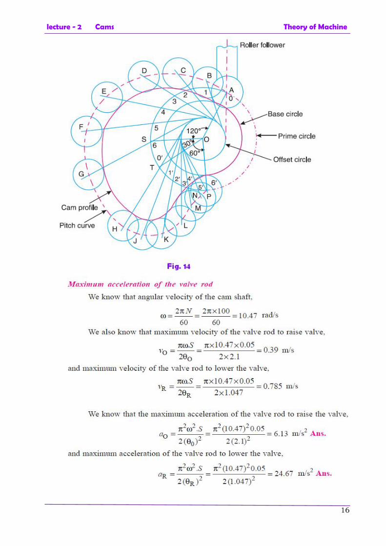
Fig. 11 (c) Acceleration diagram
(a)
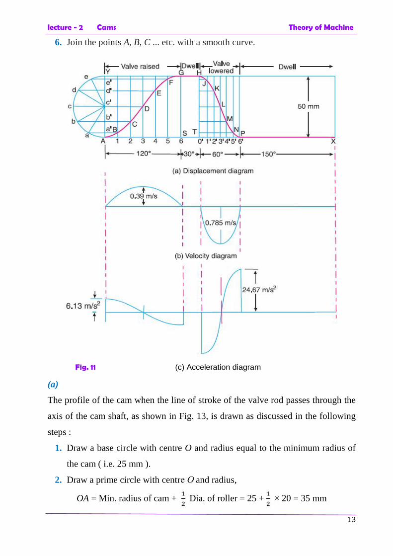
The profile of the cam when the line of stroke of the valve rod passes through the
axis of the cam shaft, as shown in Fig. 13, is drawn as discussed in the following
steps :
1. Draw a base circle with centre O and radius equal to the minimum radius of
the cam ( i.e. 25 mm ).
2. Draw a prime circle with centre O and radius,
OA = Min. radius of cam + Dia. of roller = 25 + × 20 = 35 mm
lecture - 2 Cams Theory of Machine
14
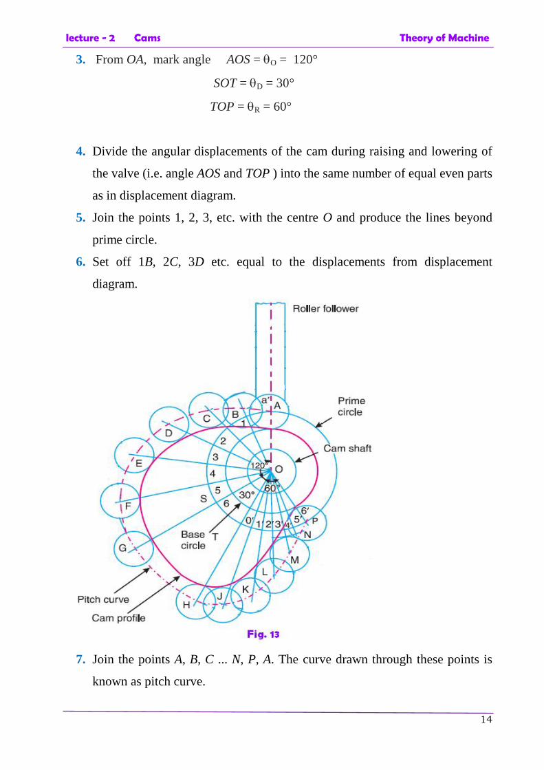
3. From OA, mark angle AOS = O = 120°
SOT = D = 30°
TOP = R = 60°
4. Divide the angular displacements of the cam during raising and lowering of
the valve (i.e. angle AOS and TOP ) into the same number of equal even parts
as in displacement diagram.
5. Join the points 1, 2, 3, etc. with the centre O and produce the lines beyond
prime circle.
6. Set off 1B, 2C, 3D etc. equal to the displacements from displacement
diagram.
7. Join the points A, B, C ... N, P, A. The curve drawn through these points is
known as pitch curve.
lecture - 2 Cams Theory of Machine
15
8. From the points A, B, C ... N, P, draw circles of radius equal to the radius of
the roller.
9. Join the bottoms of the circles with a smooth curve.
(b)
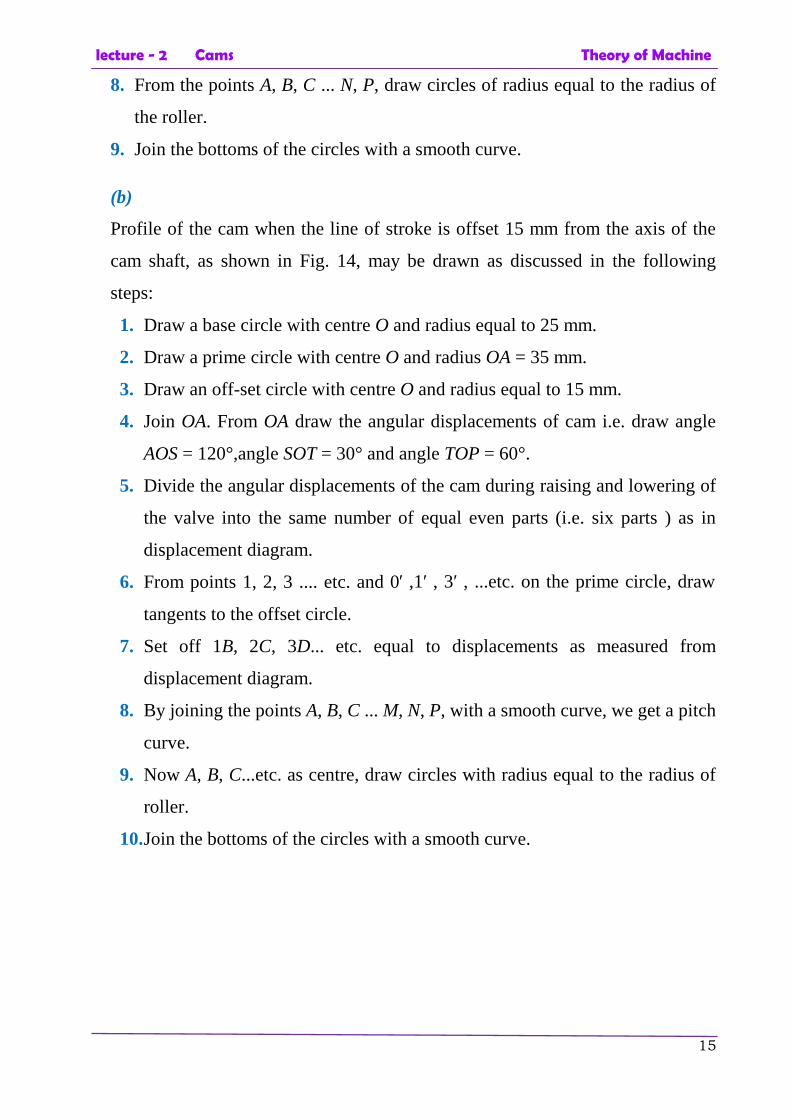
Profile of the cam when the line of stroke is offset 15 mm from the axis of the
cam shaft, as shown in Fig. 14, may be drawn as discussed in the following
steps:
1. Draw a base circle with centre O and radius equal to 25 mm.
2. Draw a prime circle with centre O and radius OA = 35 mm.
3. Draw an off-set circle with centre O and radius equal to 15 mm.
4. Join OA. From OA draw the angular displacements of cam i.e. draw angle
AOS = 120°,angle SOT = 30° and angle TOP = 60°.
5. Divide the angular displacements of the cam during raising and lowering of
the valve into the same number of equal even parts (i.e. six parts ) as in
displacement diagram.
6. From points 1, 2, 3 .... etc. and 0′ ,1′ , 3′ , ...etc. on the prime circle, draw
tangents to the offset circle.
7. Set off 1B, 2C, 3D... etc. equal to displacements as measured from
displacement diagram.
8. By joining the points A, B, C ... M, N, P, with a smooth curve, we get a pitch
curve.
9. Now A, B, C...etc. as centre, draw circles with radius equal to the radius of
roller.
10.Join the bottoms of the circles with a smooth curve.
lecture - 2 Cams Theory of Machine
16
lecture - 2 Cams Theory of Machine
17
A cam, with a minimum radius of 50 mm, rotating clockwise at a uniform speed, is
required to give a knife edge follower the motion as described below:
1. To move outwards through 40 mm during 100° rotation of the cam;
2. To dwell for next 80°;
3. To return to its starting position during next 90°, and
4. To dwell for the rest period of a revolution i.e. 90°.
Draw the profile of the cam
i. when the line of stroke of the follower passes through the centre of the cam
shaft,
ii. when the line of stroke of the follower is off-set by 15 mm.
The displacement of the follower is to take place with uniform acceleration and
uniform retardation. Determine the maximum velocity and acceleration of the
follower when the cam shaft rotates at 900 r.p.m.
Draw the displacement, velocity and acceleration diagrams for one complete
revolution of the cam.
Home Work
lecture - 3 Governors Theory of Machine
1
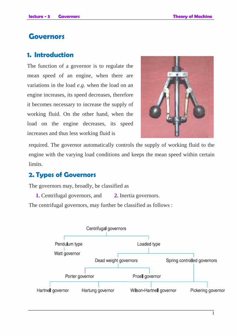
Governors
required. The governor automatically controls the supply of working fluid to the
engine with the varying load conditions and keeps the mean speed within certain
limits.
2. Types of Governors
The governors may, broadly, be classified as
1. Centrifugal governors, and 2. Inertia governors.
The centrifugal governors, may further be classified as follows :
1. Introduction
The function of a governor is to regulate the
mean speed of an engine, when there are
variations in the load e.g. when the load on an
engine increases, its speed decreases, therefore
it becomes necessary to increase the supply of
working fluid. On the other hand, when the
load on the engine decreases, its speed
increases and thus less working fluid is
lecture - 3 Governors Theory of Machine
2
3. Terms Used in Governors
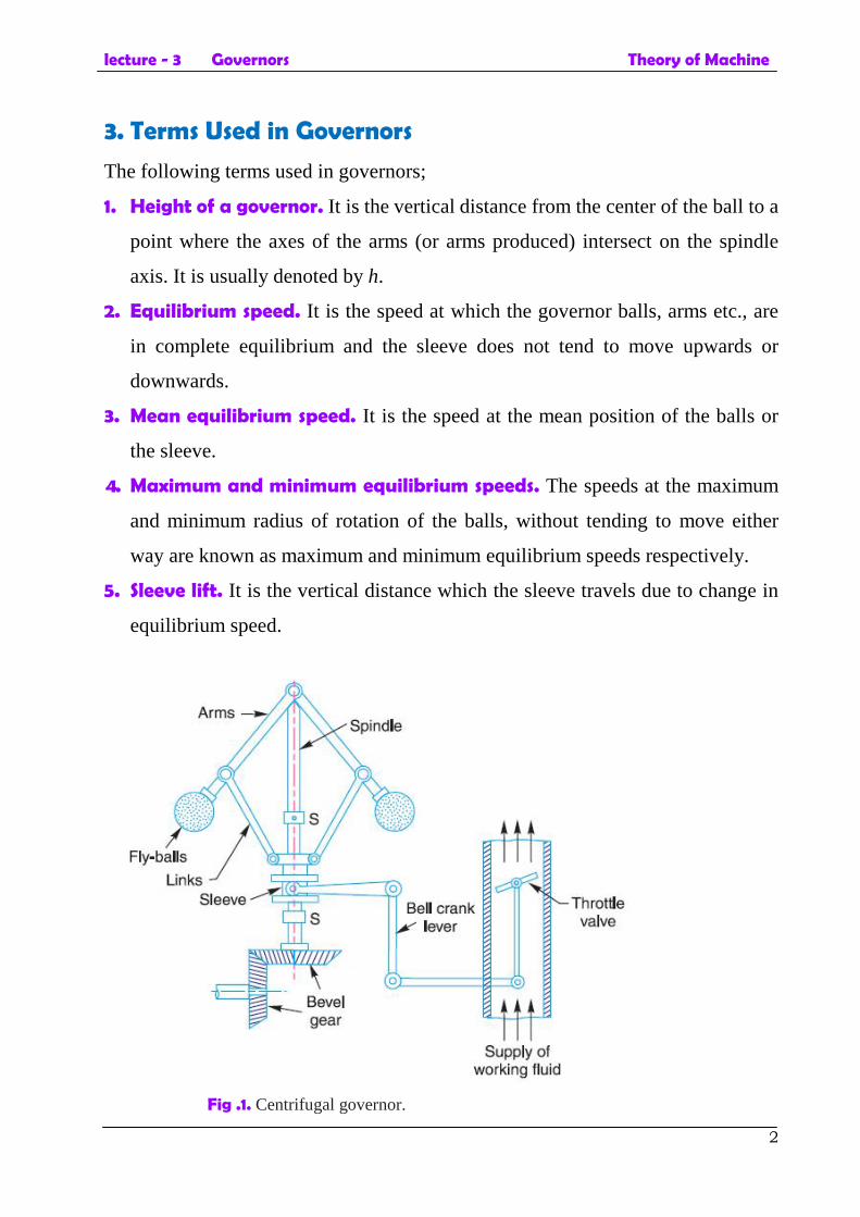
The following terms used in governors;
1. Height of a governor. It is the vertical distance from the center of the ball to a
point where the axes of the arms (or arms produced) intersect on the spindle
axis. It is usually denoted by h.
2. Equilibrium speed. It is the speed at which the governor balls, arms etc., are
in complete equilibrium and the sleeve does not tend to move upwards or
downwards.
3. Mean equilibrium speed. It is the speed at the mean position of the balls or
the sleeve.
4. Maximum and minimum equilibrium speeds. The speeds at the maximum
and minimum radius of rotation of the balls, without tending to move either
way are known as maximum and minimum equilibrium speeds respectively.
5. Sleeve lift. It is the vertical distance which the sleeve travels due to change in
equilibrium speed.
Fig .1. Centrifugal governor.
lecture - 3 Governors Theory of Machine
3
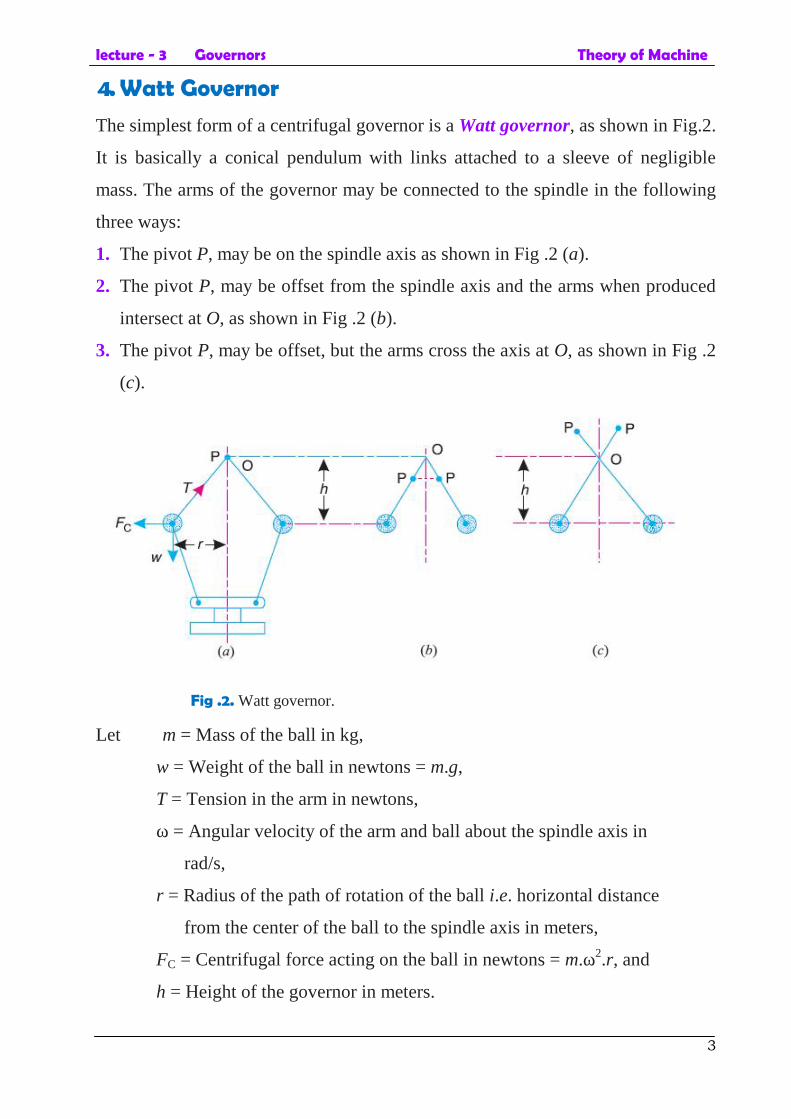
4. Watt Governor
The simplest form of a centrifugal governor is a Watt governor, as shown in Fig.2.
It is basically a conical pendulum with links attached to a sleeve of negligible
mass. The arms of the governor may be connected to the spindle in the following
three ways:
1. The pivot P, may be on the spindle axis as shown in Fig .2 (a).
2. The pivot P, may be offset from the spindle axis and the arms when produced
intersect at O, as shown in Fig .2 (b).
3. The pivot P, may be offset, but the arms cross the axis at O, as shown in Fig .2
(c).
Fig .2. Watt governor.
Let m = Mass of the ball in kg,
w = Weight of the ball in newtons = m.g,
T = Tension in the arm in newtons,
ω = Angular velocity of the arm and ball about the spindle axis in
rad/s,
r = Radius of the path of rotation of the ball i.e. horizontal distance
from the center of the ball to the spindle axis in meters,
FC = Centrifugal force acting on the ball in newtons = m.ω2.r, and
h = Height of the governor in meters.
lecture - 3 Governors Theory of Machine
4
It is assumed that the weight of the arms, links and the sleeve are negligible as
compared to the weight of the balls. Now, the ball is in equilibrium under the
action of
1. the centrifugal force (FC) acting on the ball,
2. the tension (T) in the arm, and
3. the weight (w) of the ball.
Taking moments about point O, we have
FC × h = w × r = m.g.r
or m.ω2.r.h = m.g.r or h = g /ω2 ……. (1)
Note: Watt governor may only work satisfactorily at relatively low speeds i.e.
from 60 to 80 r.p.m.
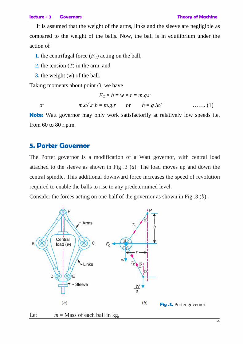
5. Porter Governor
The Porter governor is a modification of a Watt governor, with central load
attached to the sleeve as shown in Fig .3 (a). The load moves up and down the
central spindle. This additional downward force increases the speed of revolution
required to enable the balls to rise to any predetermined level.
Consider the forces acting on one-half of the governor as shown in Fig .3 (b).
Fig .3. Porter governor.
Let m = Mass of each ball in kg,
lecture - 3 Governors Theory of Machine
5
w = Weight of each ball in newtons = m.g,
M = Mass of the central load in kg,
W = Weight of the central load in newtons = M.g,
r = Radius of rotation in metres
h = Height of governor in metres ,
N = Speed of the balls in r.p.m .,
ω = Angular speed of the balls = 2 πN/60 rad/s,
FC = Centrifugal force acting on the ball in newtons = m.ω2.r,
T1 = Force in the arm in newtons,
T2 = Force in the link in newtons,
α = Angle of inclination of the arm (or upper link) to the vertical, and
β = Angle of inclination of the link (or lower link) to the vertical.
Though there are several ways of determining the relation between the height of
the governor (h) and the angular speed of the balls (ω), the following two methods
are used:
1. Method of resolution of forces ; and
2. Instantaneous centre method.
1. Method of resolution of forces
Considering the equilibrium of the forces acting at D, we have
T2 cos = =.
or T2 =.
Again, considering the equilibrium of the forces acting on B.
Fy = 0
………(1)
Fx = 0
lecture - 3 Governors Theory of Machine
6
……….(2)
Dividing equation (2) by equation (1),
Notes : 1. When the length of arms are equal to the length of links and the points P
and D lie on the same vertical line, then
tan α = tan β or q = tan α / tan β = 1
h = .
2. When the loaded sleeve moves up and down the spindle, the frictional force
acts on it in a direction opposite to that of the motion of sleeve.
If F = Frictional force acting on the sleeve
lecture - 3 Governors Theory of Machine
7
h =. . ± ( )
.
The + sign is used when the sleeve moves upwards or the governor speed increases
and –sign is used when the sleeve moves downwards or the governor speed
decreases.
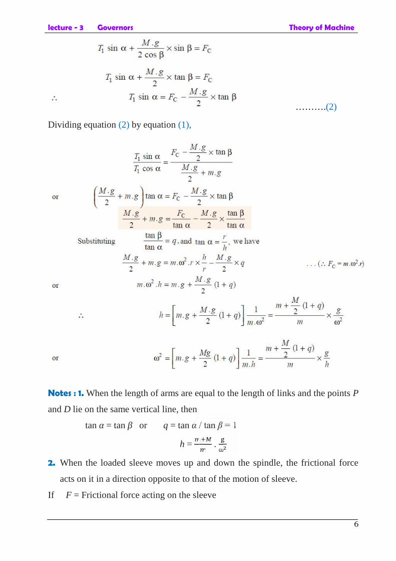
2. Instantaneous centre method
In this method, equilibrium of the forces acting on the link BD are considered. The
instantaneous centre I lies at the point of intersection of PB produced and a line
through D perpendicular to the spindle axis, as shown in Fig .4.
Taking moments about the point I,
FC × BM = w × IM + × ID
= m . g × IM +.
× ID
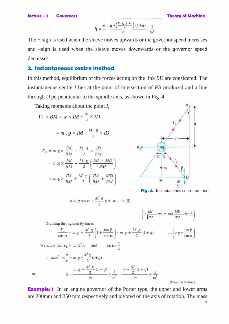
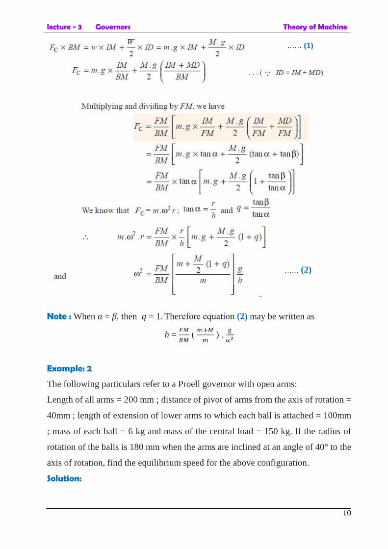
Example: 1 In an engine governor of the Porter type, the upper and lower armsare 200mm and 250 mm respectively and pivoted on the axis of rotation. The mass
Fig .4. Instantaneous centre method.
lecture - 3 Governors Theory of Machine
8
of the central load is 15 kg, the mass of each ball is 2 kg and friction of the sleevetogether with the resistance of the operating gear is equal to a load of 25 N at thesleeve. If the limiting inclinations of the upper arms to the vertical are 30° and 40°,find, taking friction into account, range of speed of the governor.
Solution:
Minimum radius of rotation,r1 = BG = BP sin 30° = 0.2 × 0.5 = 0.1 m
Height of the governor,h1 = PG = BP cos 30° = 0.2 × 0.866 = 0.1732 m
DG = (BD)2 – (BG)2 = (0.25)2 – (0.1)2 = 0.23mtan β1 = BG/DG = 0.1/0.23 = 0.4348tan α1 = tan 30° = 0.5774
q1 = =.. = 0.753
=. . ( )
.
=× . × . ( . )
. .1 = 19.2 rad/s
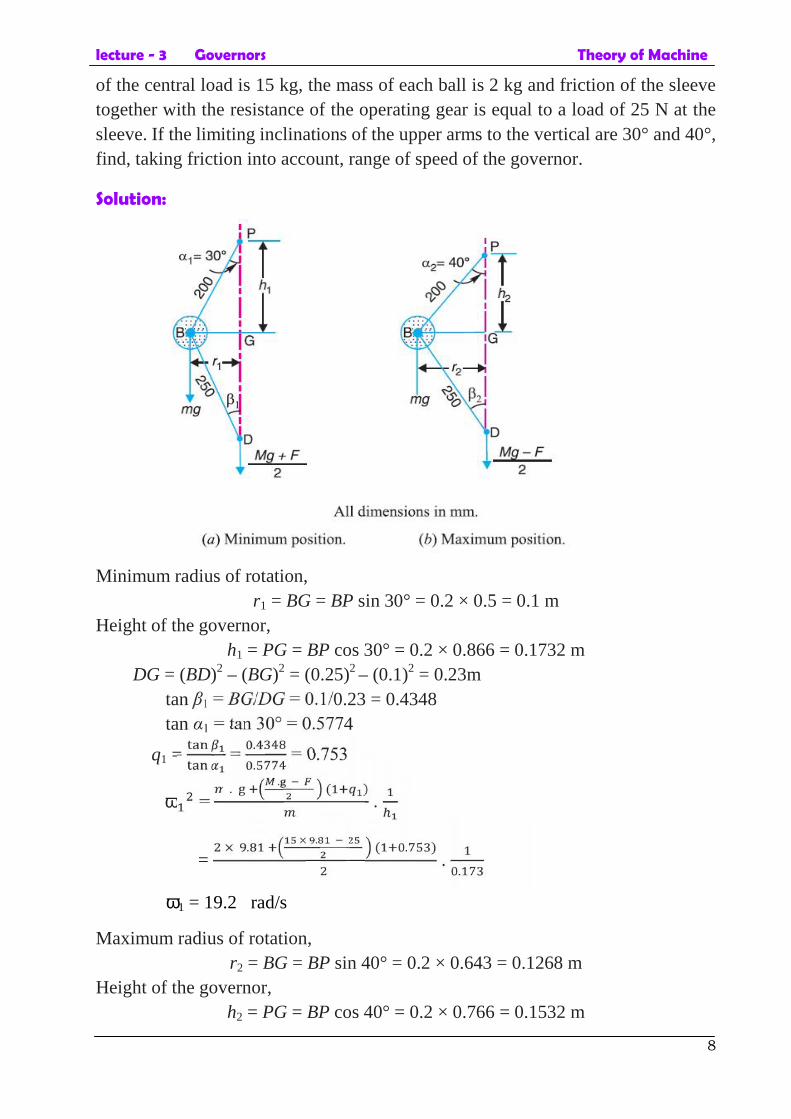
Maximum radius of rotation,r2 = BG = BP sin 40° = 0.2 × 0.643 = 0.1268 m
Height of the governor,h2 = PG = BP cos 40° = 0.2 × 0.766 = 0.1532 m
lecture - 3 Governors Theory of Machine
9
DG = (BD)2 – (BG)2 = (0.25)2 – (0.1268)2 = 0.2154 mtan β2 = BG/DG = 0.1268 / 0.2154 = 0.59
tan α2 = tan 40° = 0.839
q2 = =.. = 0.703
=. . ( )
.
=× . × . ( . )
. .2 = 23.25 rad/s
Range of speed= 2 – 1 = 23.25 – 19.2 = 4.05 rad/s Ans.
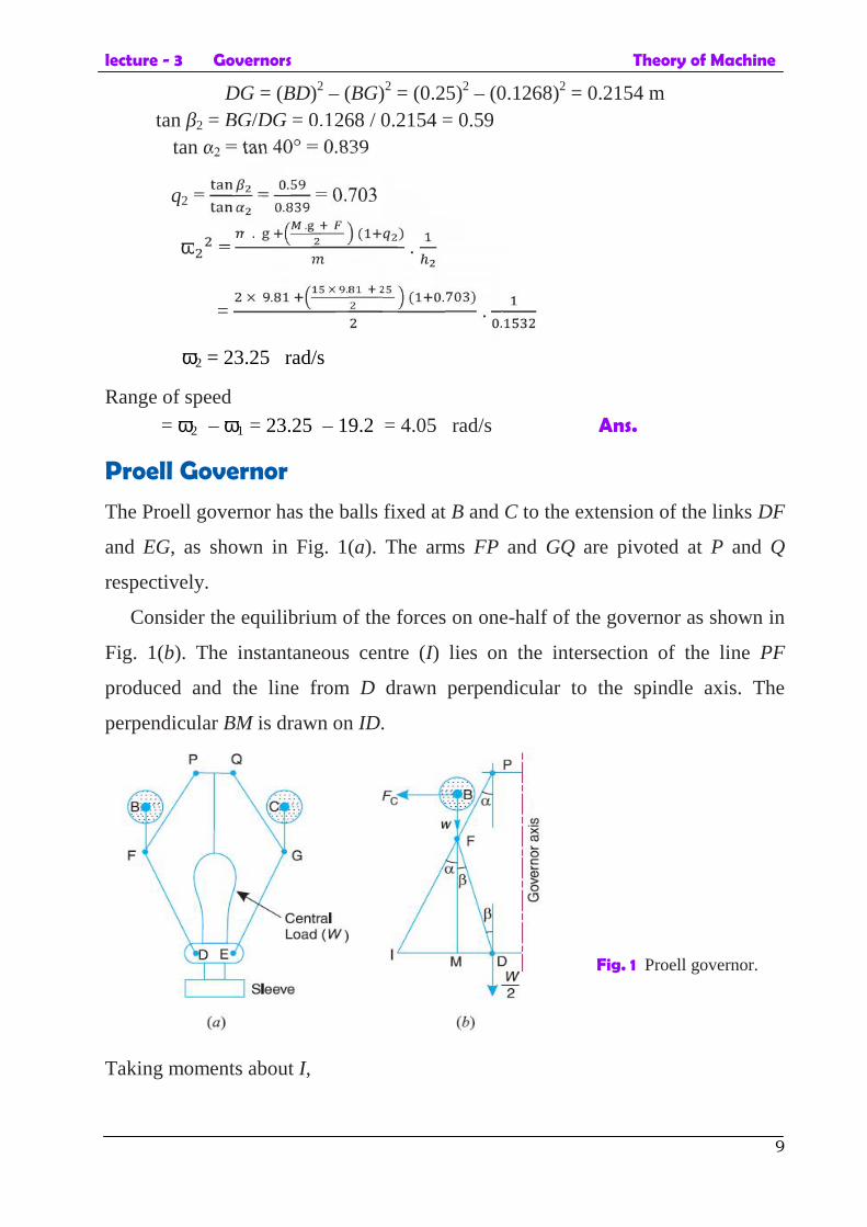
Proell Governor
The Proell governor has the balls fixed at B and C to the extension of the links DF
and EG, as shown in Fig. 1(a). The arms FP and GQ are pivoted at P and Q
respectively.
Consider the equilibrium of the forces on one-half of the governor as shown in
Fig. 1(b). The instantaneous centre (I) lies on the intersection of the line PF
produced and the line from D drawn perpendicular to the spindle axis. The
perpendicular BM is drawn on ID.
Taking moments about I,
Fig. 1 Proell governor.
lecture - 3 Governors Theory of Machine
10
Note : When α = β, then q = 1. Therefore equation (2) may be written as
h = ( ) .
Example: 2
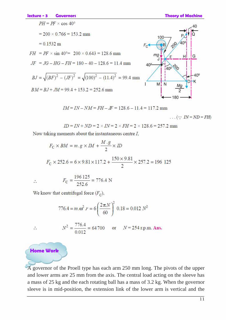
The following particulars refer to a Proell governor with open arms:
Length of all arms = 200 mm ; distance of pivot of arms from the axis of rotation =
40mm ; length of extension of lower arms to which each ball is attached = 100mm
; mass of each ball = 6 kg and mass of the central load = 150 kg. If the radius of
rotation of the balls is 180 mm when the arms are inclined at an angle of 40° to the
axis of rotation, find the equilibrium speed for the above configuration.
Solution:
…… (1)
…... (2)
lecture - 3 Governors Theory of Machine
11
A governor of the Proell type has each arm 250 mm long. The pivots of the upperand lower arms are 25 mm from the axis. The central load acting on the sleeve hasa mass of 25 kg and the each rotating ball has a mass of 3.2 kg. When the governorsleeve is in mid-position, the extension link of the lower arm is vertical and the
Home Work
lecture - 3 Governors Theory of Machine
12
radius of the path of rotation of the masses is 175 mm. The vertical height of thegovernor is 200 mm. If the governor speed is 160 r.p.m. when in mid-position,find: 1. length of the extension link; and 2. tension in the upper arm.
Answers :1. BF = 108 mm2. T= 192.5 N
lecture - 4 Gyroscopic Couple and Precessional Motion Theory of Machine
1
Gyroscopic Couple and Precessional Motion
When a body moves along a curved path with a uniform linear velocity, aforce in the direction of centripetal acceleration (known as centripetalforce) has to be applied externally over the body, so that it moves alongthe required curved path. This external force applied is known as activeforce.When a body, itself, is moving with uniform linear velocity along acircular path, it is subjected to the centrifugal force radially outwards.This centrifugal force is called reactive force. The action of the reactiveor centrifugal force is to tilt or move the body along radially outwarddirection.Centrifugal force is equal in magnitude to centripetal force but oppositein direction.
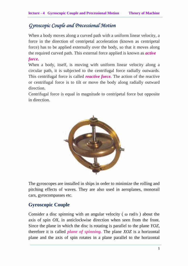
The gyroscopes are installed in ships in order to minimize the rolling andpitching effects of waves. They are also used in aeroplanes, monorailcars, gyrocompasses etc.
Gyroscopic Couple
Consider a disc spinning with an angular velocity ( ω rad/s ) about theaxis of spin OX, in anticlockwise direction when seen from the front.Since the plane in which the disc is rotating is parallel to the plane YOZ,therefore it is called plane of spinning. The plane XOZ is a horizontalplane and the axis of spin rotates in a plane parallel to the horizontal
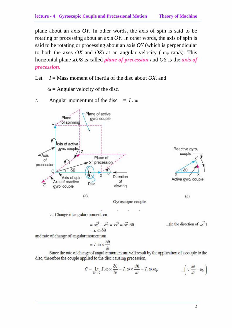
lecture - 4 Gyroscopic Couple and Precessional Motion Theory of Machine
2
plane about an axis OY. In other words, the axis of spin is said to berotating or processing about an axis OY. In other words, the axis of spin issaid to be rotating or processing about an axis OY (which is perpendicularto both the axes OX and OZ) at an angular velocity ( ωP rap/s). Thishorizontal plane XOZ is called plane of precession and OY is the axis ofprecession.
Let I = Mass moment of inertia of the disc about OX, and
ω = Angular velocity of the disc.∴ Angular momentum of the disc = I . ω
lecture - 4 Gyroscopic Couple and Precessional Motion Theory of Machine
3
Where ωP = Angular velocity of precession of the axis of spin or thespeed of rotation of the axis of spin about the axis of precession OY. Theunits of C is N-m when I is in kg-m2.
Example 1: A uniform disc of diameter 300 mm and of mass 5 kg ismounted on one end of an arm of length 600 mm. The other end of thearm is free to rotate in a universal bearing. If the disc rotates about thearm with a speed of 300 r.p.m. clockwise, looking from the front, withwhat speed will it precess about the vertical axis?
Solution:
We know that the mass moment of inertia of the disc, about an axisthrough its center of gravity and perpendicular to the plane of disc,
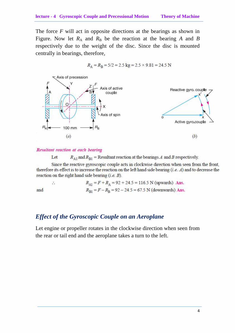
Example 2: A uniform disc of 150 mm diameter has a mass of 5 kg. Itis mounted centrally in bearings which maintain its axle in a horizontalplane. The disc spins about it axle with a constant speed of 1000 r.p.m.while the axle precesses uniformly about the vertical at 60 r.p.m. Thedirections of rotation are as shown in Figure. If the distance between thebearings is 100 mm, find the resultant reaction at each bearing due to themass and gyroscopic effects.
The direction of the reactive gyroscopic couple is shown in Figure. Let Fbe the force at each bearing due to the gyroscopic couple.
Solution:
lecture - 4 Gyroscopic Couple and Precessional Motion Theory of Machine
4
The force F will act in opposite directions at the bearings as shown inFigure. Now let RA and RB be the reaction at the bearing A and Brespectively due to the weight of the disc. Since the disc is mountedcentrally in bearings, therefore,
Effect of the Gyroscopic Couple on an Aeroplane
Let engine or propeller rotates in the clockwise direction when seen fromthe rear or tail end and the aeroplane takes a turn to the left.
lecture - 4 Gyroscopic Couple and Precessional Motion Theory of Machine
5
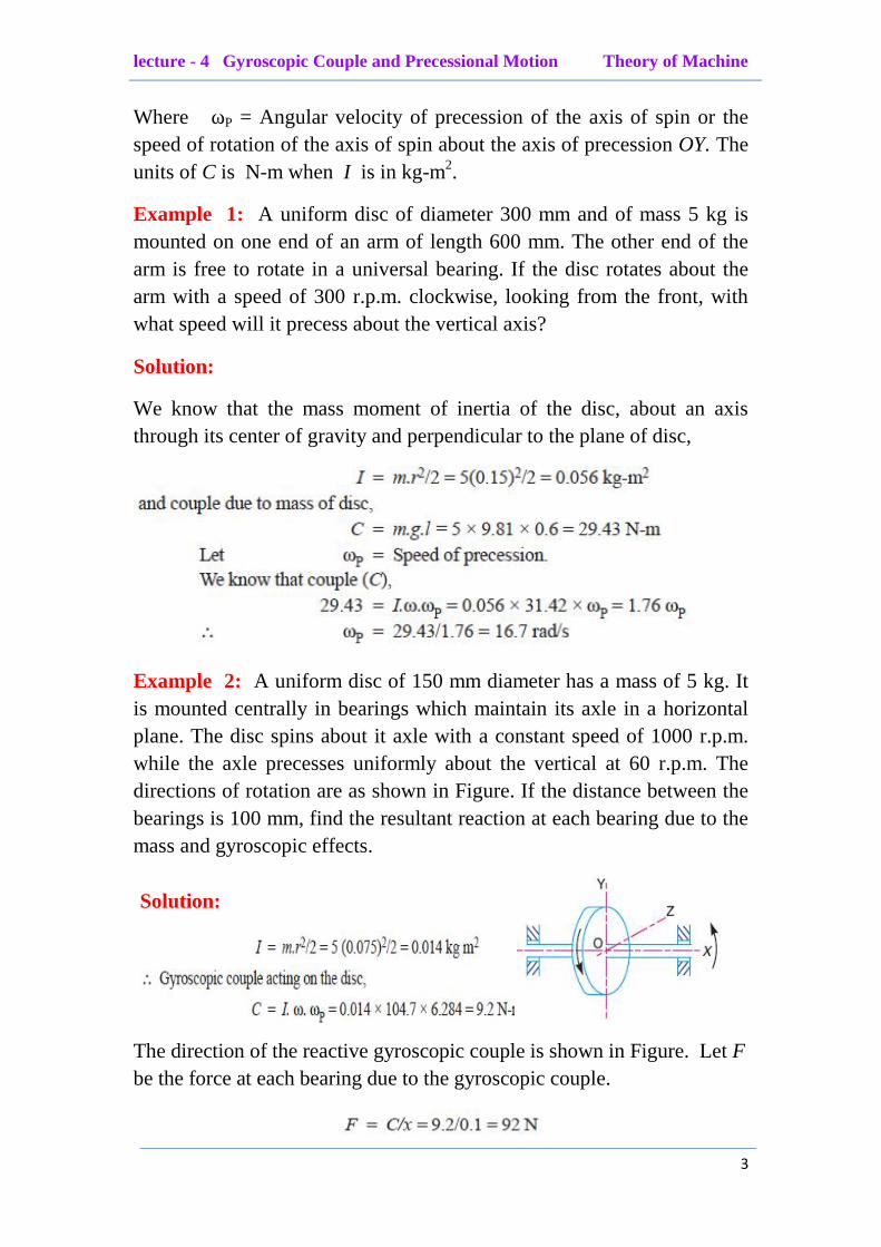
Example 3: An aeroplane makes a complete half circle of 50 metresradius, towards left, when flying at 200 km per hr. The rotary engine andthe propeller of the plane has a mass of 400 kg and a radius of gyration of0.3 m. The engine rotates at 2400 r.p.m. clockwise when viewed from therear. Find the gyroscopic couple on the aircraft and state its effect on it.
Solution: