Backpropagation - cs.cmu.edumgormley/courses/10601-s18/slides/lecture14... · 2.2.2 Backpropagation...
40
Backpropagation 1 10-601 Introduction to Machine Learning Matt Gormley Lecture 13 Mar 1, 2018 Machine Learning Department School of Computer Science Carnegie Mellon University
-
Upload
vuongquynh -
Category
Documents
-
view
217 -
download
0
Transcript of Backpropagation - cs.cmu.edumgormley/courses/10601-s18/slides/lecture14... · 2.2.2 Backpropagation...

Backpropagation
1
10-601 Introduction to Machine Learning
Matt GormleyLecture 13
Mar 1, 2018
Machine Learning DepartmentSchool of Computer ScienceCarnegie Mellon University
Reminders
• Homework 5: Neural Networks
– Out: Tue, Feb 28
– Due: Fri, Mar 9 at 11:59pm
2

Q&A
3
BACKPROPAGATION
4
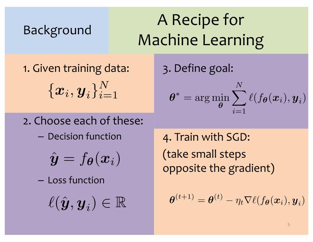
A Recipe for Machine Learning
1. Given training data: 3. Define goal:
5
Background
2. Choose each of these:– Decision function
– Loss function
4. Train with SGD:(take small steps opposite the gradient)
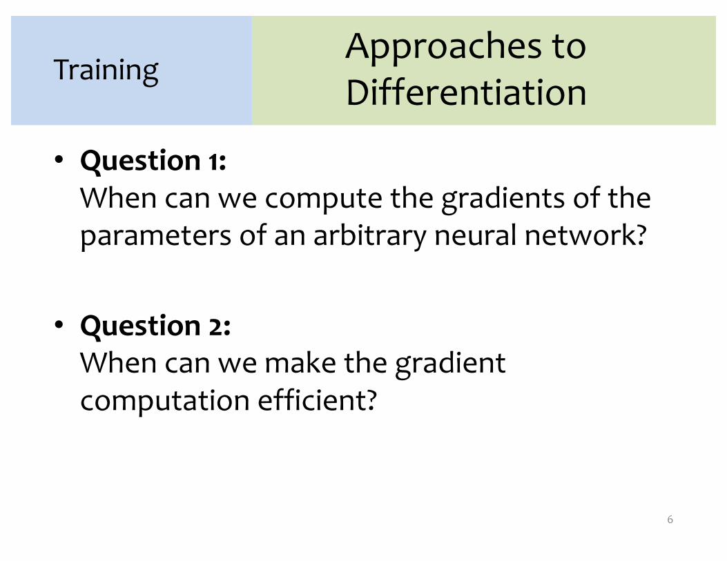
Approaches to Differentiation
• Question 1:When can we compute the gradients of the parameters of an arbitrary neural network?
• Question 2:When can we make the gradient computation efficient?
6
Training
Approaches to Differentiation
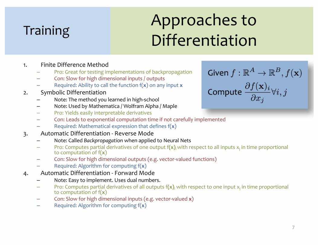
1. Finite Difference Method– Pro: Great for testing implementations of backpropagation– Con: Slow for high dimensional inputs / outputs– Required: Ability to call the function f(x) on any input x
2. Symbolic Differentiation– Note: The method you learned in high-school– Note: Used by Mathematica / Wolfram Alpha / Maple– Pro: Yields easily interpretable derivatives– Con: Leads to exponential computation time if not carefully implemented– Required: Mathematical expression that defines f(x)
3. Automatic Differentiation - Reverse Mode– Note: Called Backpropagation when applied to Neural Nets– Pro: Computes partial derivatives of one output f(x)i with respect to all inputs xj in time proportional
to computation of f(x)– Con: Slow for high dimensional outputs (e.g. vector-valued functions)– Required: Algorithm for computing f(x)
4. Automatic Differentiation - Forward Mode– Note: Easy to implement. Uses dual numbers.– Pro: Computes partial derivatives of all outputs f(x)i with respect to one input xj in time proportional
to computation of f(x)– Con: Slow for high dimensional inputs (e.g. vector-valued x)– Required: Algorithm for computing f(x)
7
Training

Finite Difference Method
Notes:• Suffers from issues of
floating point precision, in practice
• Typically only appropriate to use on small examples with an appropriately chosen epsilon
8
Training

Symbolic Differentiation
9
Training
Differentiation Quiz #1:
Suppose x = 2 and z = 3, what are dy/dx and dy/dz for the function below?

Symbolic Differentiation
Differentiation Quiz #2:
11
Training
…
…
…
Chain Rule
Whiteboard– Chain Rule of Calculus
12
Training

Chain Rule
13
Training
2.2. NEURAL NETWORKS AND BACKPROPAGATION
x to J , but also a manner of carrying out that computation in terms of the intermediatequantities a, z, b, y. Which intermediate quantities to use is a design decision. In thisway, the arithmetic circuit diagram of Figure 2.1 is differentiated from the standard neuralnetwork diagram in two ways. A standard diagram for a neural network does not show thischoice of intermediate quantities nor the form of the computations.
The topologies presented in this section are very simple. However, we will later (Chap-ter 5) how an entire algorithm can define an arithmetic circuit.
2.2.2 BackpropagationThe backpropagation algorithm (Rumelhart et al., 1986) is a general method for computingthe gradient of a neural network. Here we generalize the concept of a neural network toinclude any arithmetic circuit. Applying the backpropagation algorithm on these circuitsamounts to repeated application of the chain rule. This general algorithm goes under manyother names: automatic differentiation (AD) in the reverse mode (Griewank and Corliss,1991), analytic differentiation, module-based AD, autodiff, etc. Below we define a forwardpass, which computes the output bottom-up, and a backward pass, which computes thederivatives of all intermediate quantities top-down.
Chain Rule At the core of the backpropagation algorithm is the chain rule. The chainrule allows us to differentiate a function f defined as the composition of two functions gand h such that f = (g �h). If the inputs and outputs of g and h are vector-valued variablesthen f is as well: h : RK
! RJ and g : RJ! RI
) f : RK! RI . Given an input
vector x = {x1
, x2
, . . . , xK}, we compute the output y = {y1
, y2
, . . . , yI}, in terms of anintermediate vector u = {u
1
, u2
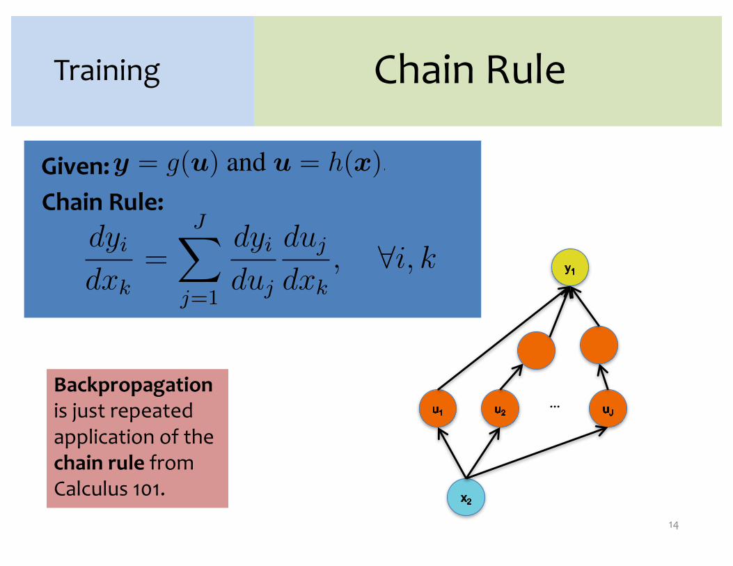
, . . . , uJ}. That is, the computation y = f(x) = g(h(x))can be described in a feed-forward manner: y = g(u) and u = h(x). Then the chain rulemust sum over all the intermediate quantities.
dyi
dxk=
JX
j=1
dyi
duj
duj
dxk, 8i, k (2.3)
If the inputs and outputs of f , g, and h are all scalars, then we obtain the familiar formof the chain rule:
dy
dx=
dy
du
du
dx(2.4)
Binary Logistic Regression Binary logistic regression can be interpreted as a arithmeticcircuit. To compute the derivative of some loss function (below we use regression) withrespect to the model parameters ✓, we can repeatedly apply the chain rule (i.e. backprop-agation). Note that the output q below is the probability that the output label takes on thevalue 1. y⇤ is the true output label. The forward pass computes the following:
J = y⇤log q + (1 � y⇤
) log(1 � q) (2.5)
where q = P✓
(Yi = 1|x) =
1
1 + exp(�
PDj=0
✓jxj)(2.6)
13
2.2. NEURAL NETWORKS AND BACKPROPAGATION
x to J , but also a manner of carrying out that computation in terms of the intermediatequantities a, z, b, y. Which intermediate quantities to use is a design decision. In thisway, the arithmetic circuit diagram of Figure 2.1 is differentiated from the standard neuralnetwork diagram in two ways. A standard diagram for a neural network does not show thischoice of intermediate quantities nor the form of the computations.
The topologies presented in this section are very simple. However, we will later (Chap-ter 5) how an entire algorithm can define an arithmetic circuit.
2.2.2 BackpropagationThe backpropagation algorithm (Rumelhart et al., 1986) is a general method for computingthe gradient of a neural network. Here we generalize the concept of a neural network toinclude any arithmetic circuit. Applying the backpropagation algorithm on these circuitsamounts to repeated application of the chain rule. This general algorithm goes under manyother names: automatic differentiation (AD) in the reverse mode (Griewank and Corliss,1991), analytic differentiation, module-based AD, autodiff, etc. Below we define a forwardpass, which computes the output bottom-up, and a backward pass, which computes thederivatives of all intermediate quantities top-down.
Chain Rule At the core of the backpropagation algorithm is the chain rule. The chainrule allows us to differentiate a function f defined as the composition of two functions gand h such that f = (g �h). If the inputs and outputs of g and h are vector-valued variablesthen f is as well: h : RK
! RJ and g : RJ! RI
) f : RK! RI . Given an input
vector x = {x1
, x2
, . . . , xK}, we compute the output y = {y1
, y2
, . . . , yI}, in terms of anintermediate vector u = {u
1
, u2
, . . . , uJ}. That is, the computation y = f(x) = g(h(x))can be described in a feed-forward manner: y = g(u) and u = h(x). Then the chain rulemust sum over all the intermediate quantities.
dyi
dxk=
JX
j=1
dyi
duj
duj
dxk, 8i, k (2.3)
If the inputs and outputs of f , g, and h are all scalars, then we obtain the familiar formof the chain rule:
dy
dx=
dy
du
du
dx(2.4)
Binary Logistic Regression Binary logistic regression can be interpreted as a arithmeticcircuit. To compute the derivative of some loss function (below we use regression) withrespect to the model parameters ✓, we can repeatedly apply the chain rule (i.e. backprop-agation). Note that the output q below is the probability that the output label takes on thevalue 1. y⇤ is the true output label. The forward pass computes the following:
J = y⇤log q + (1 � y⇤
) log(1 � q) (2.5)
where q = P✓
(Yi = 1|x) =
1
1 + exp(�
PDj=0
✓jxj)(2.6)
13
Chain Rule:
Given:
…
Chain Rule
14
Training
2.2. NEURAL NETWORKS AND BACKPROPAGATION
x to J , but also a manner of carrying out that computation in terms of the intermediatequantities a, z, b, y. Which intermediate quantities to use is a design decision. In thisway, the arithmetic circuit diagram of Figure 2.1 is differentiated from the standard neuralnetwork diagram in two ways. A standard diagram for a neural network does not show thischoice of intermediate quantities nor the form of the computations.
The topologies presented in this section are very simple. However, we will later (Chap-ter 5) how an entire algorithm can define an arithmetic circuit.
2.2.2 BackpropagationThe backpropagation algorithm (Rumelhart et al., 1986) is a general method for computingthe gradient of a neural network. Here we generalize the concept of a neural network toinclude any arithmetic circuit. Applying the backpropagation algorithm on these circuitsamounts to repeated application of the chain rule. This general algorithm goes under manyother names: automatic differentiation (AD) in the reverse mode (Griewank and Corliss,1991), analytic differentiation, module-based AD, autodiff, etc. Below we define a forwardpass, which computes the output bottom-up, and a backward pass, which computes thederivatives of all intermediate quantities top-down.
Chain Rule At the core of the backpropagation algorithm is the chain rule. The chainrule allows us to differentiate a function f defined as the composition of two functions gand h such that f = (g �h). If the inputs and outputs of g and h are vector-valued variablesthen f is as well: h : RK
! RJ and g : RJ! RI
) f : RK! RI . Given an input
vector x = {x1
, x2
, . . . , xK}, we compute the output y = {y1
, y2
, . . . , yI}, in terms of anintermediate vector u = {u
1
, u2
, . . . , uJ}. That is, the computation y = f(x) = g(h(x))can be described in a feed-forward manner: y = g(u) and u = h(x). Then the chain rulemust sum over all the intermediate quantities.
dyi
dxk=
JX
j=1
dyi
duj
duj
dxk, 8i, k (2.3)
If the inputs and outputs of f , g, and h are all scalars, then we obtain the familiar formof the chain rule:
dy
dx=
dy
du
du
dx(2.4)
Binary Logistic Regression Binary logistic regression can be interpreted as a arithmeticcircuit. To compute the derivative of some loss function (below we use regression) withrespect to the model parameters ✓, we can repeatedly apply the chain rule (i.e. backprop-agation). Note that the output q below is the probability that the output label takes on thevalue 1. y⇤ is the true output label. The forward pass computes the following:
J = y⇤log q + (1 � y⇤
) log(1 � q) (2.5)
where q = P✓
(Yi = 1|x) =
1
1 + exp(�
PDj=0
✓jxj)(2.6)
13
Chain Rule:
Given:
…
Backpropagationis just repeated application of the chain rule from Calculus 101.

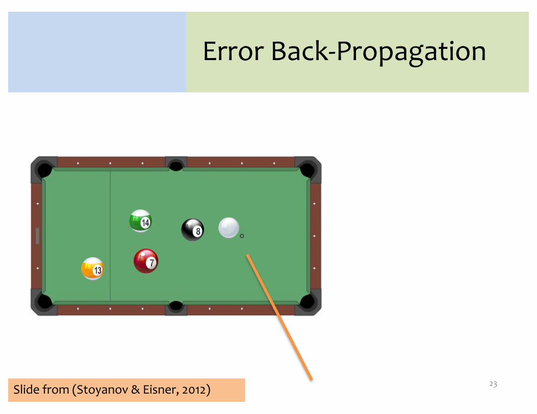
Error Back-Propagation
15Slide from (Stoyanov & Eisner, 2012)

Error Back-Propagation
16Slide from (Stoyanov & Eisner, 2012)

Error Back-Propagation
17Slide from (Stoyanov & Eisner, 2012)

Error Back-Propagation
18Slide from (Stoyanov & Eisner, 2012)
Error Back-Propagation
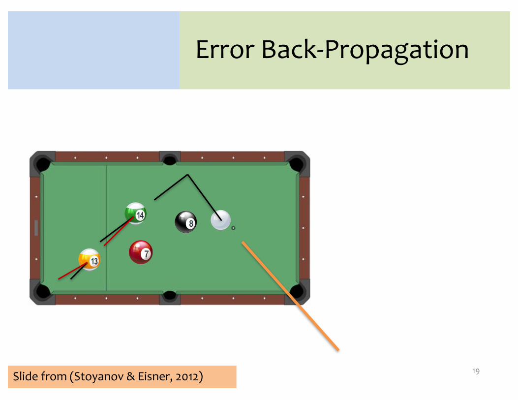
19Slide from (Stoyanov & Eisner, 2012)
Error Back-Propagation
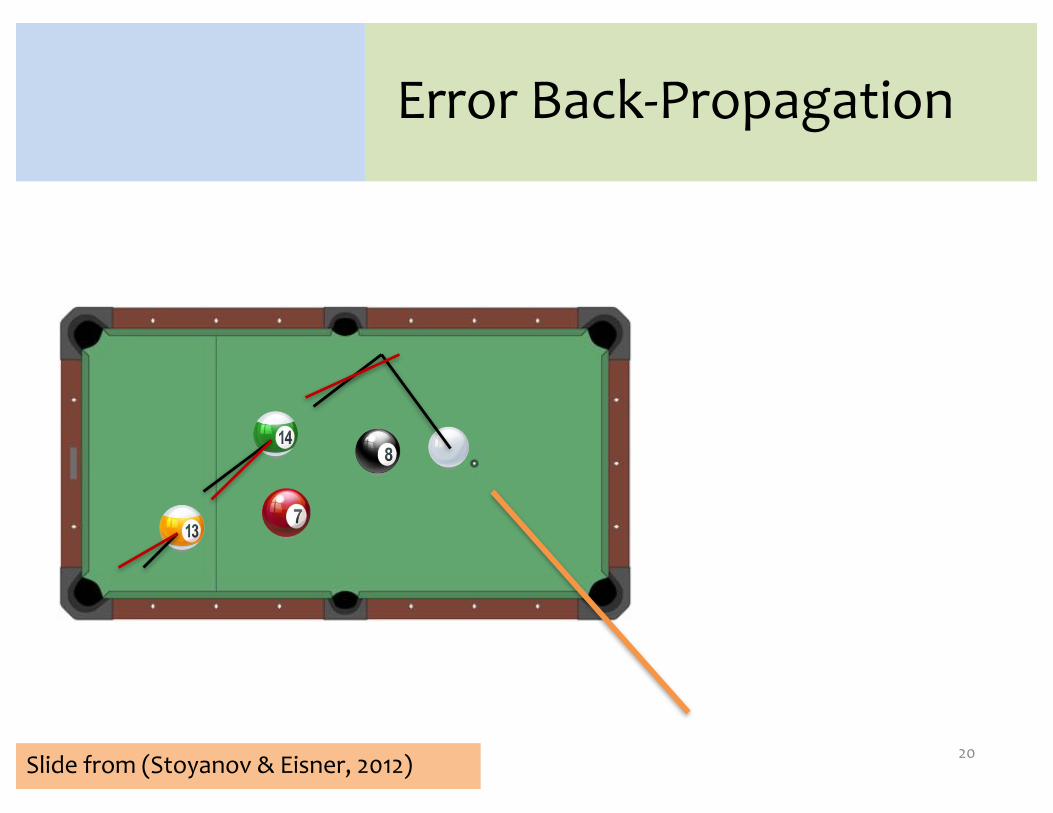
20Slide from (Stoyanov & Eisner, 2012)

Error Back-Propagation
21Slide from (Stoyanov & Eisner, 2012)

Error Back-Propagation
22Slide from (Stoyanov & Eisner, 2012)
Error Back-Propagation
23Slide from (Stoyanov & Eisner, 2012)

Error Back-Propagation
24
y(i)
p(y|x(i))
z
ϴ
Slide from (Stoyanov & Eisner, 2012)
Backpropagation
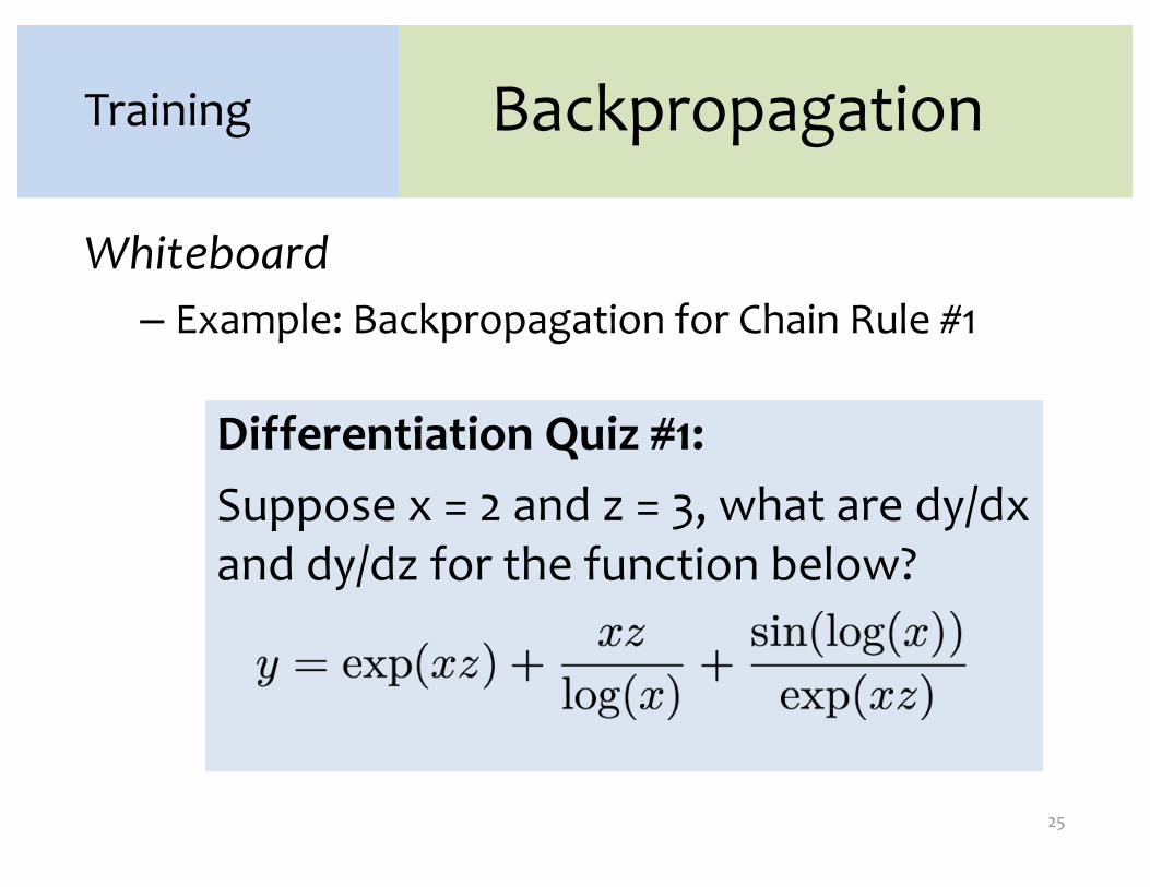
Whiteboard– Example: Backpropagation for Chain Rule #1
25
Training
Differentiation Quiz #1:
Suppose x = 2 and z = 3, what are dy/dx and dy/dz for the function below?
Backpropagation
26
Training
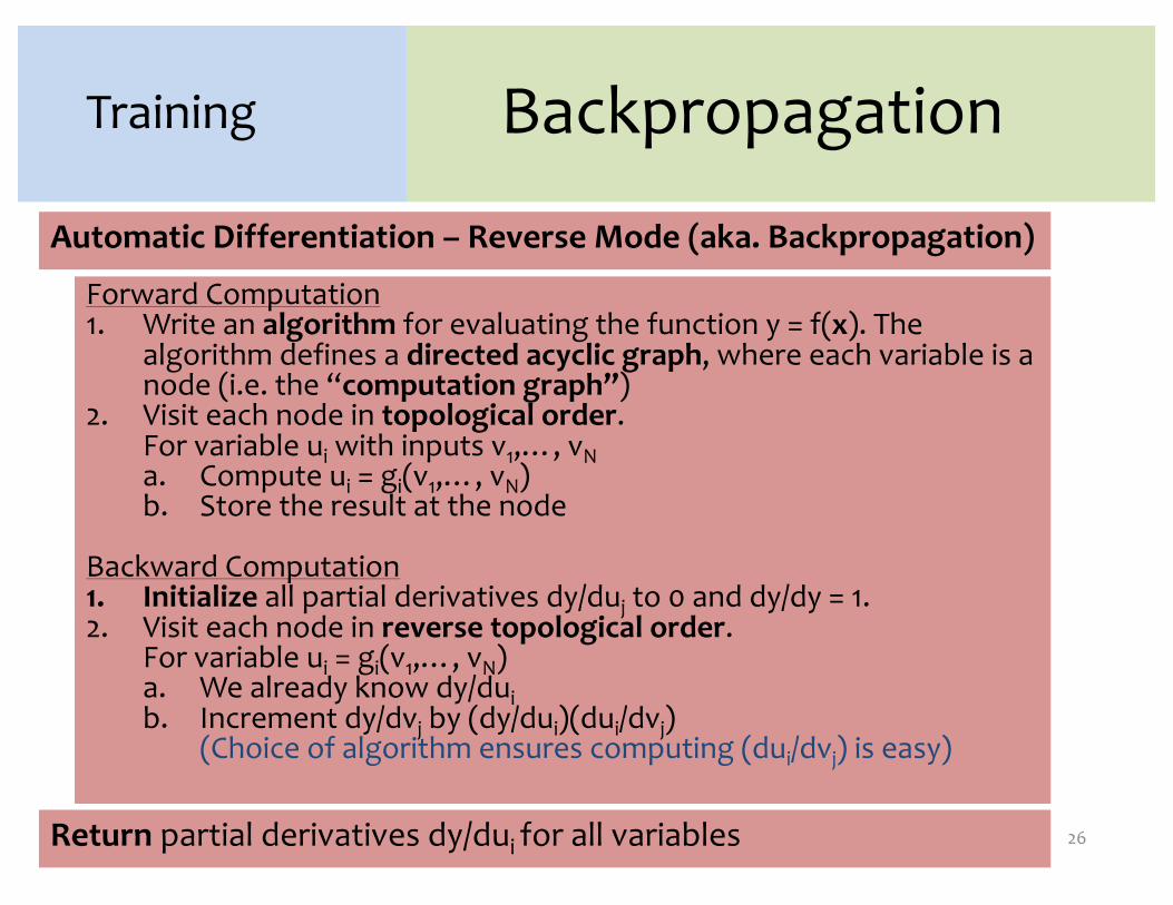
Automatic Differentiation – Reverse Mode (aka. Backpropagation)
Forward Computation1. Write an algorithm for evaluating the function y = f(x). The
algorithm defines a directed acyclic graph, where each variable is a node (i.e. the “computation graph”)
2. Visit each node in topological order. For variable ui with inputs v1,…, vNa. Compute ui = gi(v1,…, vN)b. Store the result at the node
Backward Computation1. Initialize all partial derivatives dy/duj to 0 and dy/dy = 1.2. Visit each node in reverse topological order.
For variable ui = gi(v1,…, vN)a. We already know dy/duib. Increment dy/dvj by (dy/dui)(dui/dvj)
(Choice of algorithm ensures computing (dui/dvj) is easy)
Return partial derivatives dy/dui for all variables

Backpropagation
27
Training
Forward Backward
J = cos(u)dJ
du= �sin(u)
u = u1 + u2dJ
du1=
dJ
du
du
du1,
du
du1= 1
dJ
du2=
dJ
du
du
du2,
du
du2= 1
u1 = sin(t)dJ
dt=
dJ
du1
du1
dt,
du1
dt= (t)
u2 = 3tdJ
dt=
dJ
du2
du2
dt,
du2
dt= 3
t = x2 dJ
dx=
dJ
dt
dt
dx,
dt
dx= 2x
Simple Example: The goal is to compute J = ( (x2) + 3x2)on the forward pass and the derivative dJ
dx on the backward pass.

Backpropagation
28
Training
Forward Backward
J = cos(u)dJ
du= �sin(u)
u = u1 + u2dJ
du1=
dJ
du
du
du1,
du
du1= 1
dJ
du2=
dJ
du
du
du2,
du
du2= 1
u1 = sin(t)dJ
dt=
dJ
du1
du1
dt,
du1
dt= (t)
u2 = 3tdJ
dt=
dJ
du2
du2
dt,
du2
dt= 3
t = x2 dJ
dx=
dJ
dt
dt
dx,
dt
dx= 2x
Simple Example: The goal is to compute J = ( (x2) + 3x2)on the forward pass and the derivative dJ
dx on the backward pass.

Backpropagation
29
Training
…
Output
Input
θ1 θ2 θ3 θM
Case 1:Logistic Regression
Forward Backward
J = y� y + (1 � y�) (1 � y)dJ
dy=
y�
y+
(1 � y�)
y � 1
y =1
1 + (�a)
dJ
da=
dJ
dy
dy
da,
dy
da=
(�a)
( (�a) + 1)2
a =D�
j=0
�jxjdJ
d�j=
dJ
da
da
d�j,
da
d�j= xj
dJ
dxj=
dJ
da
da
dxj,
da
dxj= �j

Backpropagation
30
Training
…
…
Output
Input
Hidden Layer
(F) LossJ = 1
2 (y � y(d))2
(E) Output (sigmoid)y = 1
1+ (�b)
(D) Output (linear)b =
�Dj=0 �jzj
(C) Hidden (sigmoid)zj = 1
1+ (�aj), �j
(B) Hidden (linear)aj =
�Mi=0 �jixi, �j
(A) InputGiven xi, �i

Backpropagation
31
Training
…
…
Output
Input
Hidden Layer
(F) LossJ = 1
2 (y � y�)2
(E) Output (sigmoid)y = 1
1+ (�b)
(D) Output (linear)b =
�Dj=0 �jzj
(C) Hidden (sigmoid)zj = 1
1+ (�aj), �j
(B) Hidden (linear)aj =
�Mi=0 �jixi, �j
(A) InputGiven xi, �i
Backpropagation
32
Training
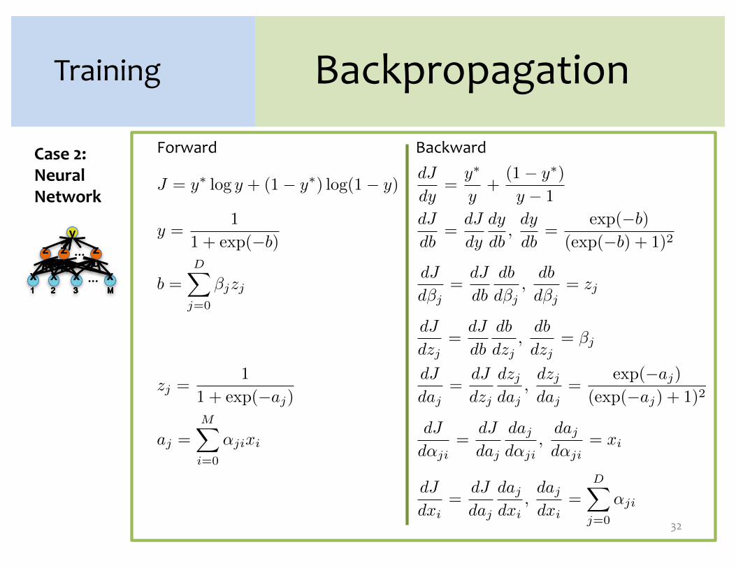
Case 2:Neural Network
…
…
Forward Backward
J = y� y + (1 � y�) (1 � y)dJ
dy=
y�
y+
(1 � y�)
y � 1
y =1
1 + (�b)
dJ
db=
dJ
dy
dy
db,
dy
db=
(�b)
( (�b) + 1)2
b =D�
j=0
�jzjdJ
d�j=
dJ
db
db
d�j,
db
d�j= zj
dJ
dzj=
dJ
db
db
dzj,
db
dzj= �j
zj =1
1 + (�aj)
dJ
daj=
dJ
dzj
dzj
daj,
dzj
daj=
(�aj)
( (�aj) + 1)2
aj =M�
i=0
�jixidJ
d�ji=
dJ
daj
daj
d�ji,
daj
d�ji= xi
dJ
dxi=
dJ
daj
daj
dxi,
daj
dxi=
D�
j=0
�ji
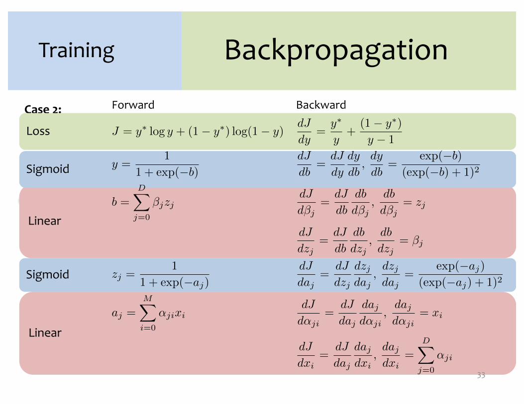
Case 2:Neural Network
…
…
Linear
Sigmoid
Linear
Sigmoid
Loss
Backpropagation
33
Training
Forward Backward
J = y� y + (1 � y�) (1 � y)dJ
dy=
y�
y+
(1 � y�)
y � 1
y =1
1 + (�b)
dJ
db=
dJ
dy
dy
db,
dy
db=
(�b)
( (�b) + 1)2
b =D�
j=0
�jzjdJ
d�j=
dJ
db
db
d�j,
db
d�j= zj
dJ
dzj=
dJ
db
db
dzj,
db
dzj= �j
zj =1
1 + (�aj)
dJ
daj=
dJ
dzj
dzj
daj,
dzj
daj=
(�aj)
( (�aj) + 1)2
aj =M�
i=0
�jixidJ
d�ji=
dJ
daj
daj
d�ji,
daj
d�ji= xi
dJ
dxi=
dJ
daj
daj
dxi,
daj
dxi=
D�
j=0
�ji

Derivative of a Sigmoid
34

Case 2:Neural Network
…
…
Linear
Sigmoid
Linear
Sigmoid
Loss
Backpropagation
35
Training
Forward Backward
J = y� y + (1 � y�) (1 � y)dJ
dy=
y�
y+
(1 � y�)
y � 1
y =1
1 + (�b)
dJ
db=
dJ
dy
dy
db,
dy
db=
(�b)
( (�b) + 1)2
b =D�
j=0
�jzjdJ
d�j=
dJ
db
db
d�j,
db
d�j= zj
dJ
dzj=
dJ
db
db
dzj,
db
dzj= �j
zj =1
1 + (�aj)
dJ
daj=
dJ
dzj
dzj
daj,
dzj
daj=
(�aj)
( (�aj) + 1)2
aj =M�
i=0
�jixidJ
d�ji=
dJ
daj
daj
d�ji,
daj
d�ji= xi
dJ
dxi=
dJ
daj
daj
dxi,
daj
dxi=
D�
j=0
�ji

Case 2:Neural Network
…
…
Linear
Sigmoid
Linear
Sigmoid
Loss
Backpropagation
36
Training

Backpropagation
Whiteboard– SGD for Neural Network– Example: Backpropagation for Neural Network
37
Training

Backpropagation
38
Training
Backpropagation (Auto.Diff. - Reverse Mode)
Forward Computation1. Write an algorithm for evaluating the function y = f(x). The
algorithm defines a directed acyclic graph, where each variable is a node (i.e. the “computation graph”)
2. Visit each node in topological order. a. Compute the corresponding variable’s valueb. Store the result at the node
Backward Computation1. Initialize all partial derivatives dy/duj to 0 and dy/dy = 1.2. Visit each node in reverse topological order.
For variable ui = gi(v1,…, vN)a. We already know dy/duib. Increment dy/dvj by (dy/dui)(dui/dvj)
(Choice of algorithm ensures computing (dui/dvj) is easy)
Return partial derivatives dy/dui for all variables
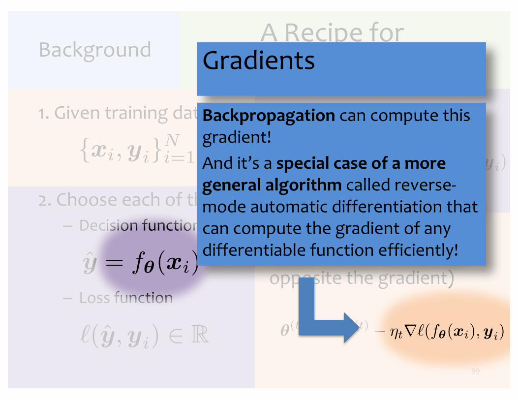
A Recipe for Machine Learning
1. Given training data: 3. Define goal:
39
Background
2. Choose each of these:– Decision function
– Loss function
4. Train with SGD:(take small steps opposite the gradient)
Gradients
Backpropagation can compute this gradient! And it’s a special case of a more general algorithm called reverse-mode automatic differentiation that can compute the gradient of any differentiable function efficiently!

Summary
1. Neural Networks…– provide a way of learning features– are highly nonlinear prediction functions– (can be) a highly parallel network of logistic
regression classifiers– discover useful hidden representations of the
input2. Backpropagation…– provides an efficient way to compute gradients– is a special case of reverse-mode automatic
differentiation40
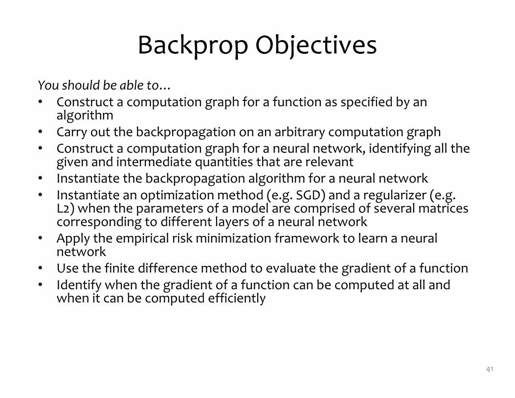
Backprop ObjectivesYou should be able to…• Construct a computation graph for a function as specified by an
algorithm• Carry out the backpropagation on an arbitrary computation graph• Construct a computation graph for a neural network, identifying all the
given and intermediate quantities that are relevant• Instantiate the backpropagation algorithm for a neural network• Instantiate an optimization method (e.g. SGD) and a regularizer (e.g.
L2) when the parameters of a model are comprised of several matrices corresponding to different layers of a neural network
• Apply the empirical risk minimization framework to learn a neural network
• Use the finite difference method to evaluate the gradient of a function• Identify when the gradient of a function can be computed at all and
when it can be computed efficiently
41