Background Knowledge

Brief Review on Brief Review on

• Counting, Counting,

• Probability, Probability,

• Statistics, Statistics,

• I. Theory I. Theory

Counting: Permutations

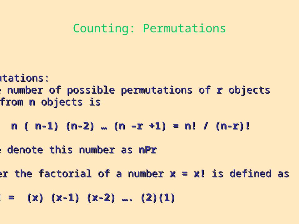
Permutations:Permutations:The number of possible permutations of The number of possible permutations of rr objects objects from from nn objects is objects is

n ( n-1) (n-2) … (n –r +1) = n! / (n-r)!n ( n-1) (n-2) … (n –r +1) = n! / (n-r)!

We denote this number as We denote this number as nPrnPr

Remember the factorial of a number Remember the factorial of a number x = x!x = x! is defined as is defined as

x! = (x) (x-1) (x-2) …. (2)(1)x! = (x) (x-1) (x-2) …. (2)(1)

Counting: Permutations

Permutations with indistinguishable objects:Permutations with indistinguishable objects:

Assume we have a total of Assume we have a total of nn objects. objects.

r1r1 are alike, are alike, r2r2 are alike,.., are alike,.., rkrk are alike. are alike.

The number of possible permutations of The number of possible permutations of nn objects is objects is n! / r1! r2! … rk!n! / r1! r2! … rk!

Counting: Combinations

Combinations:Combinations: Assume we wish to select Assume we wish to select rr objects from objects from nn objects. objects. In this case we do not care about the order in In this case we do not care about the order in which we select the which we select the rr objects. objects. The number of possible combinations of The number of possible combinations of rr objects objects from from nn objects is objects is n ( n-1) (n-2) … (n –r +1) / r! = n! / (n-r)! r!n ( n-1) (n-2) … (n –r +1) / r! = n! / (n-r)! r!

We denote this number as We denote this number as C(n,r)C(n,r)

Statistical and Inductive Probability

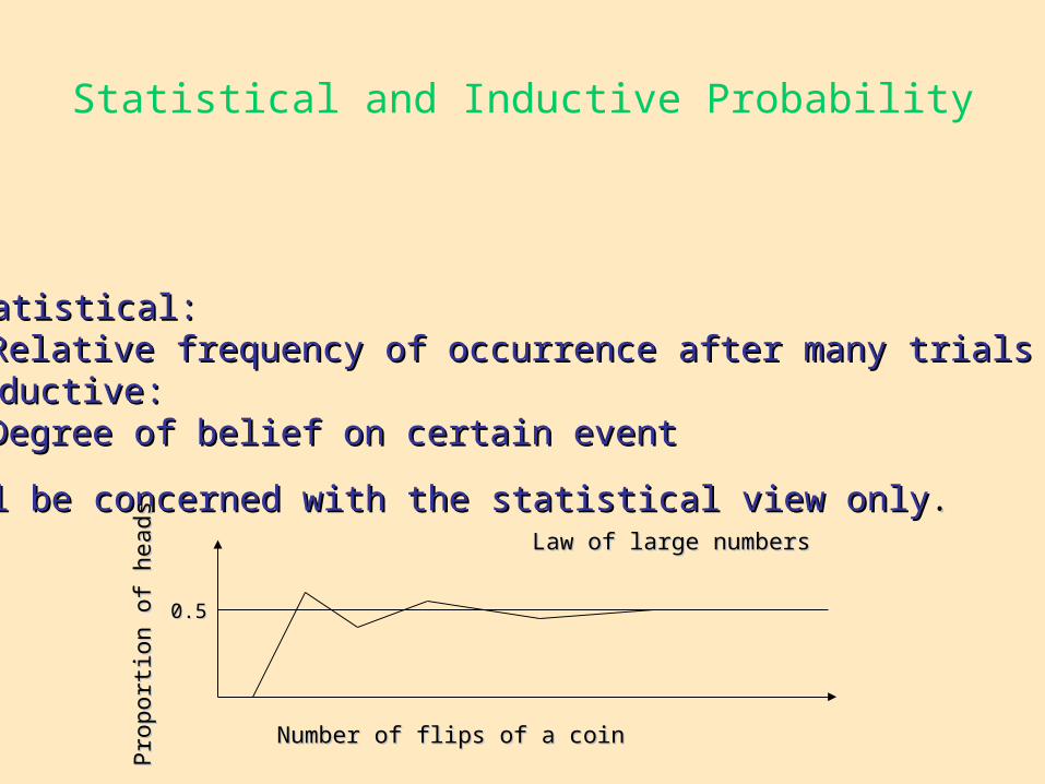
Statistical:Statistical:Relative frequency of occurrence after many trialsRelative frequency of occurrence after many trials

Inductive:Inductive:Degree of belief on certain eventDegree of belief on certain event

We will be concerned with the statistical view onlyWe will be concerned with the statistical view only..

0.50.5

Number of flips of a coinNumber of flips of a coin

Pro

port

ion

of h

eads

Pro

port

ion

of h

eads Law of large numbersLaw of large numbers

The Sample Space

The space of all possible outcomes of a given process The space of all possible outcomes of a given process or situation is called the sample space or situation is called the sample space SS..

Example: cars crossing a check point based on color and sizeExample: cars crossing a check point based on color and size::

SS

red & smallred & small blue & smallblue & small

red & largered & large blue & largeblue & large

An Event

An event is a subset of the sample space. An event is a subset of the sample space.

Example: Event Example: Event AA: red cars crossing a check point : red cars crossing a check point irrespective of sizeirrespective of size

SS

red & smallred & small blue & smallblue & small

red & largered & large blue & largeblue & largeAA

The Laws of Probability

The probability of the sample space The probability of the sample space SS is 1, is 1, P(S)P(S) = 1 = 1The probability of any event The probability of any event AA is such that is such that 0 <= P(A) <= 10 <= P(A) <= 1. . Law of AdditionLaw of AdditionIf If AA and and BB are mutually exclusive events, then the probability that are mutually exclusive events, then the probability that either one of them will occur is the sum of the individual probabilities:either one of them will occur is the sum of the individual probabilities:

P(A or B) = P(A) + P(B)P(A or B) = P(A) + P(B)

If If AA and and BB are not mutually exclusive: are not mutually exclusive:

P(A or B) = P(A) + P(B) – P(A and B)P(A or B) = P(A) + P(B) – P(A and B)AA

BB

Conditional Probabilities

Given that Given that AA and and BB are events in sample space are events in sample space SS, and , and P(B)P(B) is is different of 0, then the conditional probability of different of 0, then the conditional probability of AA given given BB is is

P(A|B) = P(A and B) / P(B)P(A|B) = P(A and B) / P(B)

If If AA and and BB are independent then are independent then P(A|B) = P(A)P(A|B) = P(A)

The Laws of Probability

Law of MultiplicationLaw of Multiplication

What is the probability that both What is the probability that both AA and and BB occur together? occur together? P(A and B) = P(A) P(B|A)P(A and B) = P(A) P(B|A) where where P(B|A)P(B|A) is the probability of is the probability of BB conditioned on conditioned on AA..

If If AA and and BB are statistically independent: are statistically independent: P(B|A) = P(B)P(B|A) = P(B) and then and then P(A and B) = P(A) P(B) P(A and B) = P(A) P(B)

Random Variable

Definition: A variable that can take on several values, Definition: A variable that can take on several values, each value having a probability of occurrence. each value having a probability of occurrence.

There are two types of random variables:There are two types of random variables:Discrete. Discrete. Take on a countable number of values. Take on a countable number of values.Continuous. Continuous. Take on a range of values. Take on a range of values.

Discrete VariablesDiscrete Variables For every discrete variable For every discrete variable XX there will be a probability function there will be a probability function P(x) = P(X = x).P(x) = P(X = x). The cumulative probability function for The cumulative probability function for XX is defined as is defined as F(x) = P(X <= x).F(x) = P(X <= x).

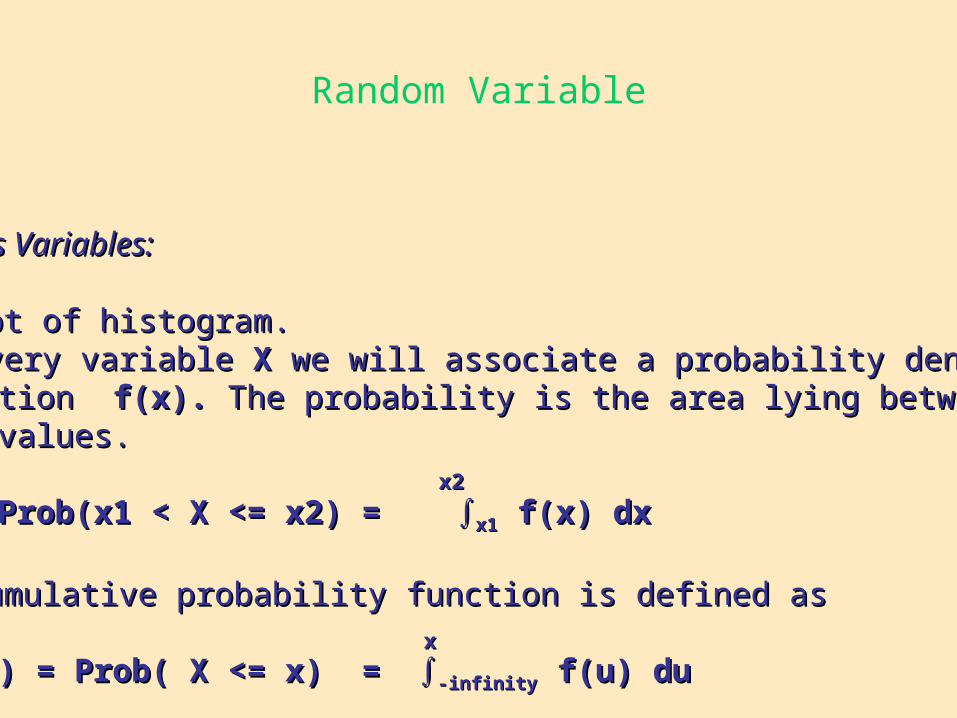
Random Variable

Continuous Variables:Continuous Variables:

Concept of histogram.Concept of histogram. For every variable For every variable XX we will associate a probability density we will associate a probability density function function f(x).f(x). The probability is the area lying between The probability is the area lying between two values.two values.

Prob(x1 < X <= x2) = ∫Prob(x1 < X <= x2) = ∫x1x1 f(x) dx f(x) dx

The cumulative probability function is defined as The cumulative probability function is defined as

F(x) = Prob( X <= x) = ∫F(x) = Prob( X <= x) = ∫-infinity-infinity f(u) du f(u) du

x2x2

xx

Multivariate Distributions

P(x,y) = P( X = x and Y = y).P(x,y) = P( X = x and Y = y).

P’(x) = Prob( X = x) = P’(x) = Prob( X = x) = ∑∑yy P(x,y) P(x,y)

It is called the marginal distribution of It is called the marginal distribution of XX The same can be done on The same can be done on YY to define the marginal to define the marginal distribution of distribution of Y, P”(y).Y, P”(y).

If X and Y are independent thenIf X and Y are independent then P(x,y) = P’(x) P”(y)P(x,y) = P’(x) P”(y)

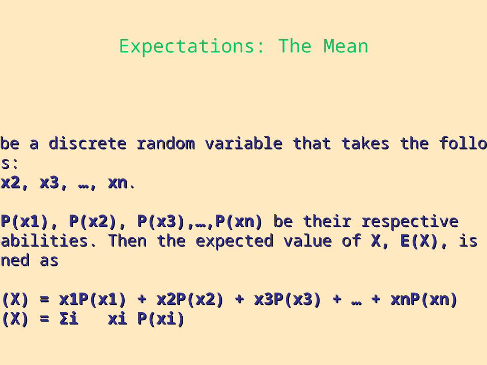
Expectations: The Mean

Let Let XX be a discrete random variable that takes the following be a discrete random variable that takes the following values: values: x1, x2, x3, …, xnx1, x2, x3, …, xn. .

Let Let P(x1), P(x2), P(x3),…,P(xn)P(x1), P(x2), P(x3),…,P(xn) be their respective be their respective probabilities. Then the expected value of probabilities. Then the expected value of X, E(X),X, E(X), is is defined asdefined as

E(X) = x1P(x1) + x2P(x2) + x3P(x3) + … + xnP(xn)E(X) = x1P(x1) + x2P(x2) + x3P(x3) + … + xnP(xn) E(X) = Σi xi P(xi)E(X) = Σi xi P(xi)

The Binomial Distribution

What is the probability of getting x successes in n trials?What is the probability of getting x successes in n trials? Assumption: all trials are independent and the probability of Assumption: all trials are independent and the probability of success remains the same. success remains the same.

Let Let pp be the probability of success and let be the probability of success and let q = 1-pq = 1-p

then the binomial distribution is defined asthen the binomial distribution is defined as

P(x) = P(x) = nnCCxx p p xx q q n-x n-x for x = 0,1,2,…,nfor x = 0,1,2,…,n

The mean equals The mean equals n pn p

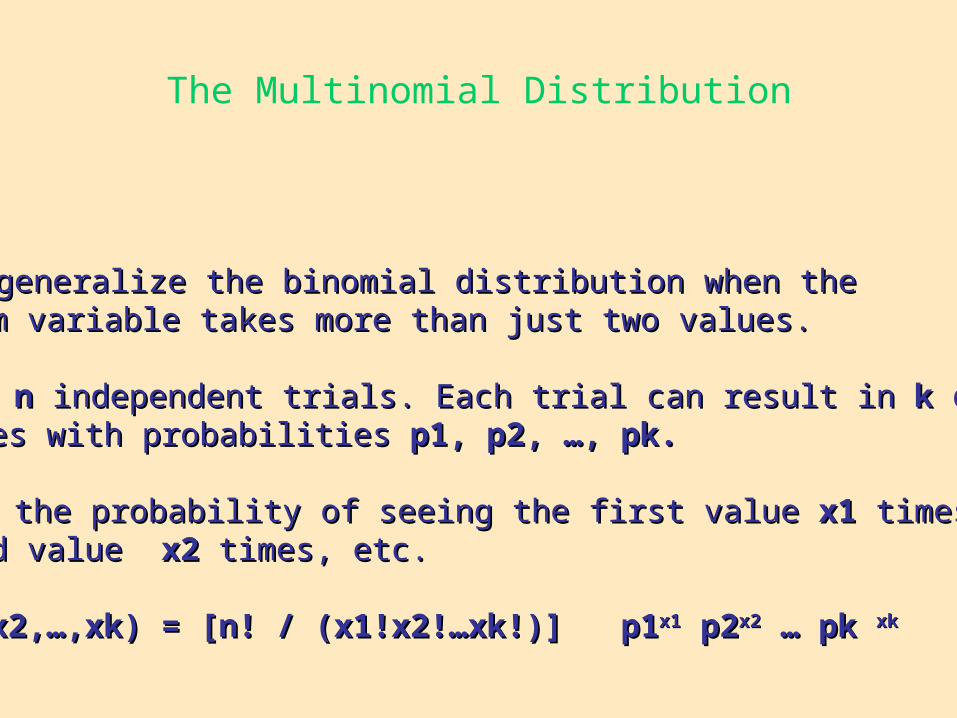
The Multinomial Distribution

We can generalize the binomial distribution when theWe can generalize the binomial distribution when the random variable takes more than just two values. random variable takes more than just two values.

We have We have nn independent trials. Each trial can result in independent trials. Each trial can result in kk different different values with probabilities values with probabilities p1, p2, …, pk.p1, p2, …, pk.

What is the probability of seeing the first value What is the probability of seeing the first value x1x1 times, the times, the second value second value x2x2 times, etc. times, etc.

P(x1,x2,…,xk) = [n! / (x1!x2!…xk!)] p1P(x1,x2,…,xk) = [n! / (x1!x2!…xk!)] p1x1x1 p2 p2x2x2 … pk … pk xkxk

Other Distributions

PoissonPoisson P(x) = eP(x) = e-u -u uux x / x!/ x! GeometricGeometric

f(x) = p(1-p)f(x) = p(1-p)x-1x-1

ExponentialExponentialf(x) = λ ef(x) = λ e-λx-λx

Others:Others: NormalNormal χχ22, , tt, and , and FF

Entropy of a Random Variable

A measure of uncertainty or entropy that is associated A measure of uncertainty or entropy that is associated to a random variable X is defined as to a random variable X is defined as

H(X) = - Σ pi log piH(X) = - Σ pi log pi

where the logarithm is in base 2.where the logarithm is in base 2.

This is the “average amount of information or entropy of a finiteThis is the “average amount of information or entropy of a finitecomplete probability scheme” (Introduction to I. Theory by Reza F.).complete probability scheme” (Introduction to I. Theory by Reza F.).

Example of Entropy

P(A) = 1/256, P(B) = 255/256P(A) = 1/256, P(B) = 255/256 H(X) = 0.0369 bitH(X) = 0.0369 bit

P(A) = 1/2, P(B) = 1/2P(A) = 1/2, P(B) = 1/2 H(X) = 1 bitH(X) = 1 bit

P(A) = 7/16, P(B) = 9/16P(A) = 7/16, P(B) = 9/16 H(X) = 0.989 bitH(X) = 0.989 bit

There are two possible complete events There are two possible complete events AA and and BB(Example: flipping a biased coin). (Example: flipping a biased coin).

Entropy of a Binary Source

It is a function concave downward. It is a function concave downward.

00 0.50.5 11

1 bit1 bit

Derived Measures

Average information per pairsAverage information per pairs H(X,Y) = - ΣxΣy P(x,y) log P(x,y)H(X,Y) = - ΣxΣy P(x,y) log P(x,y)

Conditional Entropy:Conditional Entropy:H(X|Y) = - ΣxΣy P(x,y) log P(x|y)H(X|Y) = - ΣxΣy P(x,y) log P(x|y)

Mutual Information:Mutual Information:I(X;Y) = ΣxΣy P(x,y) log [P(x,y) / (P(x) P(y))]I(X;Y) = ΣxΣy P(x,y) log [P(x,y) / (P(x) P(y))] = H(X) + H(Y) – H(X,Y)= H(X) + H(Y) – H(X,Y)

= H(X) – H(X|Y)= H(X) – H(X|Y) = H(Y) – H(Y|X)= H(Y) – H(Y|X)