BACK TEST MODELING AND ANALYSIS

OF DYNAMIC FX INDICES

Worcester Polytechnic Institute- Major Qualifying Project

John Paul Syriopoulos Antonio Talledo

December 15th 2011

2

Abstract

This project involves the implementation of Dynamic Foreign Exchange Indices

with MATLAB programming software. We developed a generic template in MATLAB

that will be used as a tool by the Royal Bank of Scotland Foreign Exchange Structuring

Desk to create and modify FX indices more effective and efficiently. Besides the time

savings and convenience, the new MATLAB tool with also enable the Structuring desk to

offer more complex indices to its retail clients due to its greater computing power relative

to Excel.

3

Executive Summary

The foreign exchange market is continuing to grow rapidly and within it the FX

Index business is becoming more critical with time. The FX Structuring desk at Royal

Bank of Scotland realized that in order to improve their solutions to their clients they

needed to become a bigger player in the index world and therefore should start building

better and more powerful tools to build their own indices. Having historically used

Microsoft Excel to build indices, RBS recognized that it wasn’t the ideal program to use

and decided that using a programming language called MATLAB could offer them a way

to create a new framework to create, and manage a new breed of FX indices that will help

their clients achieve their goals.

Our final product consisted of a tool created with MATLAB, which offers a

framework to build new indices and modify existing ones. As opposed to an Excel

document with multiple spreadsheets, the tools looks like a page of code composed of

multiple instructions and commands. We used a particular index, commonly known as

the G10 Smart Carry Index, as a base to build the tool since this Index had been built in

Excel by RBS right before our arrival. Our project consisted of first developing a

thorough understanding of what indices are and how they work. To have a good

foundation, we first developed a couple of small indices in Excel. The second part of the

project consisted of building the G10 Smart Carry index in Excel. Finally, we started

designing the index using MATLAB and from then on we kept refining it until we had

the last product.

4

This project was a great challenge for us in many aspects. First of all, our

experience with MATLAB prior to this project had been extremely limited. Therefore, a

significant challenge was to learn the programming language, which usually takes a long

time to polish. Another significant challenge worth mentioning was the unplanned

departure of our project manager on our second week on the term. He was the only

person in the team involved with the team. Therefore, helping our new manager catch up

with our work, and actually teaching him what we had learned so far was an interesting

dynamic. However, ironically our new manager turned out to be an excellent programmer

and within weeks he was able to help us significantly throughout our project.

5

Acknowledgements

We would like to thank the following people, who each provided guidance and support to

our project.

RBS FX Structuring Team

Richard Groenewegen

Ben Nicklin

John Quayle

David Popplewell

Professor Arthur Gerstenfeld

Professor Justin Wang

6

Table of Contents

Table of Tables…………………………………………………..………………………..7

Table of Figures…………………………………………………..……………………….7

Project Context and Introduction…………………………………...……………………..9

Background……………………………………………………………..………………..13

Royal Bank of Scotland…………………………………………...……………..13

Literature Review…………………………………………………….…………..14

Back-testing and Analysis of Dynamic FX Indices Project……………………….……..23

Project Overview……………………………………………….……………………..…23

Index Methodology………………………………………………...…………………….23

Beta Indices Methodology. ………………………..…………………………………….29

Excel Construction…………………………………...…………………………………..33

Construction of index in Matlab…………………………………………………………37

The Matlab Tool vs Excel………………………………………………………………..48

Matlab Tool and Variations……………………….……………………………………..58

Project Impact and Conclusions…………………………………...……………………..68

Appendix…………………………………………………………………………………71

References

Table of Tables

Table 1: G10 currencies and symbol…………………………………………….………24

Table 2: Constituents…………………………………………………………….………29

7

Table 3: Dynamic Exposure……………………………………………...………………36

Table 4: Performance Statistics……………………………………….…………………61

Table 5: Original Dynamic Exposure……………………………………………………64

Table 6: Modified Dynamic Exposure………………………………………...…………64

Table 7: Performance Statistics II………………………………………………..………65

Table of Figures

Figure 1: Average Daily FX Turnover ($ bn) …………………………………...………9

Figure 2: P&L of Forward Contract……………………….………………………..……18

Figure 3: Overall Index Structure: …………………………………………...………… 25

Figure 4: Core Index Structure……………………………………………………..……26

Figure 5: Final Index Structure…………………………………………………………..27

Figure 6: EURUSD Index……………………………………………………………..…31

Figure 7: 1m Forward Rates USDEUR………………………………….………………32

Figure 8: Core Index Object………………………………………………………..……40

Figure 9: Core Index Underlying Data……………………………………..……………41

Figure 10: Matrices………………………………………………………………………43

Figure 11: Indexing Matrix………………………………………………………………44

Figure 12: Index Positioning…………………………………………………..…………46

Figure 13: Index Positioning II…………………………………………..………………46

Figure 14: Underlying Data Matrix………………………………………………...……47

8

Figure 15: Step 1 – Add Calculation Dates……………………………...………………49

Figure 16: Step 2- Insert data using VLOOKUP function…………………………….…50

Figure 17: Step 3- Calculate Average……………………………………………………51

Figure 18: Step 1…………………………………………………………………………52

Figure 19: Step 2…………………………………………………………………………53

Figure 20: Step 3…………………………………………………………………………54

Figure 21: MyIndex……………………………………………………………...………55

Figure 22: Complete Matrix…………………….………………………….……………56

Figure 23: Diagram of Implied Rate Calculation……………..…………………………59

Figure 24: Performance using implied vs actual rate………………….…………………60

Figure 25: Performance illustrating leverage levels…………………………..…………60

Figure 26: Volatility of the two indices…………………………………………….……61

Figure 27: Modified vs Original Dynamic Exposure……………………………………65

9

1. Project Context and Introduction

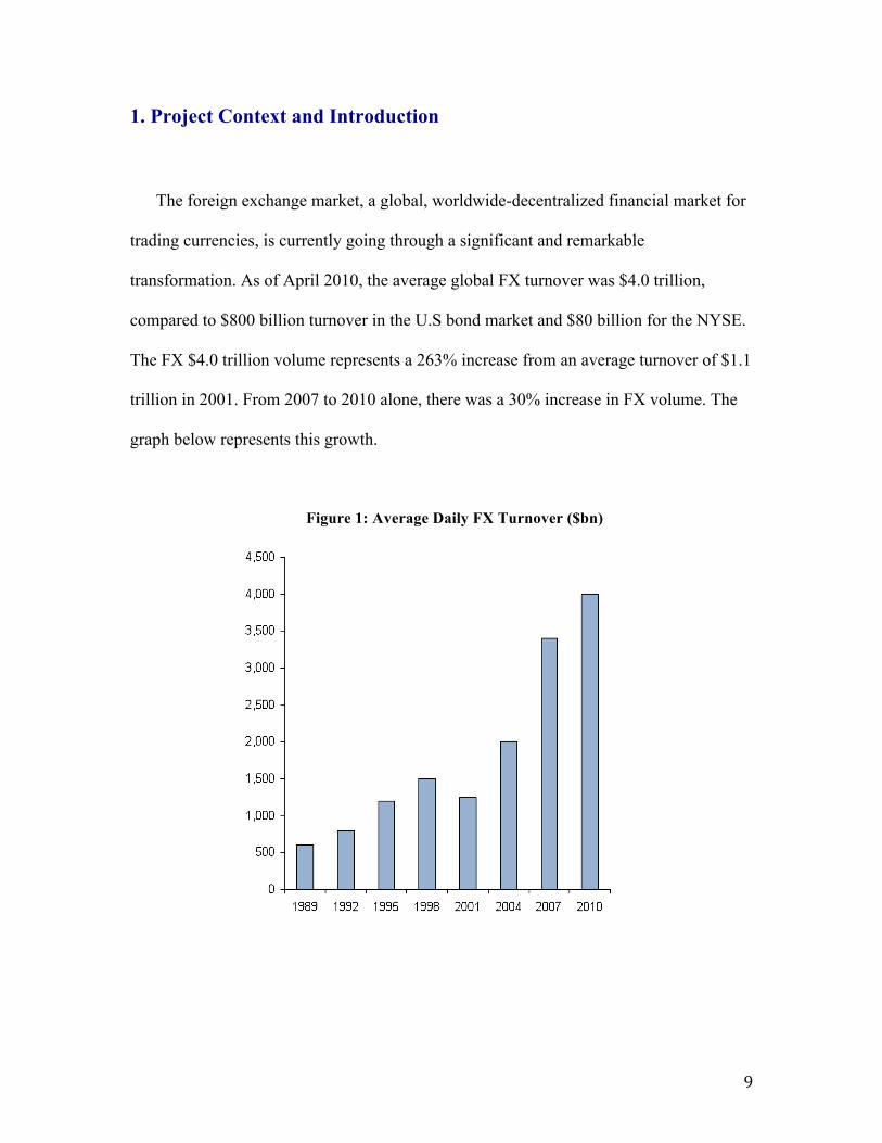
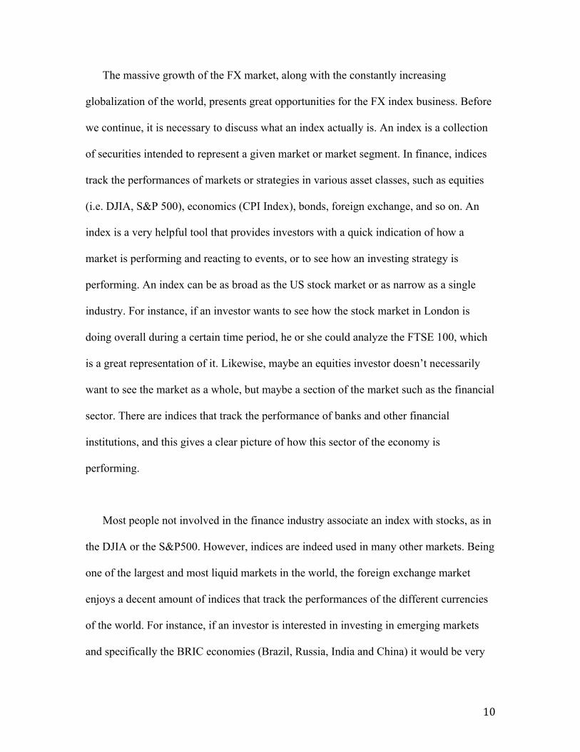
The foreign exchange market, a global, worldwide-decentralized financial market for

trading currencies, is currently going through a significant and remarkable

transformation. As of April 2010, the average global FX turnover was $4.0 trillion,

compared to $800 billion turnover in the U.S bond market and $80 billion for the NYSE.

The FX $4.0 trillion volume represents a 263% increase from an average turnover of $1.1

trillion in 2001. From 2007 to 2010 alone, there was a 30% increase in FX volume. The

graph below represents this growth.

Figure 1: Average Daily FX Turnover ($bn)

10

The massive growth of the FX market, along with the constantly increasing

globalization of the world, presents great opportunities for the FX index business. Before

we continue, it is necessary to discuss what an index actually is. An index is a collection

of securities intended to represent a given market or market segment. In finance, indices

track the performances of markets or strategies in various asset classes, such as equities

(i.e. DJIA, S&P 500), economics (CPI Index), bonds, foreign exchange, and so on. An

index is a very helpful tool that provides investors with a quick indication of how a

market is performing and reacting to events, or to see how an investing strategy is

performing. An index can be as broad as the US stock market or as narrow as a single

industry. For instance, if an investor wants to see how the stock market in London is

doing overall during a certain time period, he or she could analyze the FTSE 100, which

is a great representation of it. Likewise, maybe an equities investor doesn’t necessarily

want to see the market as a whole, but maybe a section of the market such as the financial

sector. There are indices that track the performance of banks and other financial

institutions, and this gives a clear picture of how this sector of the economy is

performing.

Most people not involved in the finance industry associate an index with stocks, as in

the DJIA or the S&P500. However, indices are indeed used in many other markets. Being

one of the largest and most liquid markets in the world, the foreign exchange market

enjoys a decent amount of indices that track the performances of the different currencies

of the world. For instance, if an investor is interested in investing in emerging markets

and specifically the BRIC economies (Brazil, Russia, India and China) it would be very

11

useful for him to see a BRIC vs. USD Index, which would show the performance of a

basket of the four currencies against the US Dollar. In fact, what makes indices so

valuable is that they serve not solely as indicators, or benchmarks, but most of them are

tradable. This means that someone can invest on the index and the returns will be equal to

the performance of that index. Clients may want to trade foreign exchange indices for

many reasons, of which four stand out: Firstly, for simplicity. FX indices give an investor

the ability to trade a basket of currencies (the G10, for instance) at the click of a button.

Second, indices can act as a currency benchmark to hedge a portfolio of assets or to

express a view about a country’s macroeconomic outlook will affect its currency.

Another reason might be to speculate- a position in a basket of currencies will provide

diversification benefits due to decreased volatility. Finally, an essential reason why a

client might want to trade indices is for hedging purposes. If a company has exposure to

multiple currencies, such as a multinational company like Procter & Gamble or

McDonalds, hedging all of them simultaneously via indices rather than individually will

be significantly cheaper as well as operationally efficient.

A booming FX market places the index business in a critical time, since they provide

diverse and cost effective market access for investors. Each year, due to increased

globalization, more companies produce and sell their products in foreign markets and

therefore become more exposed to the FX market. In order to hedge their exposure, these

companies are in need of market intelligence and are demanding FX indices to aid them

with their hedging decisions. In order to respond to the needs of their clients, banks such

12

as RBS create tradable indices in which their clients can transact their hedges and protect

them from fluctuations in exchange rates.

Currently, however, RBS is not yet big player in this sector, though it certainly

has the potential to enter more aggressively and become one. In order to do this, it is

necessary to have the right tools that will give them the ability to provide the most

insightful and effective indices to their clients. The nature of the FX Structuring desk is

dealing with bespoke and unique requests for clients and setting up the best deal that will

suit them. With FX Indices this is certainly the case and therefore having the correct tools

and systems will allow RBS to satisfy their clients with their special needs. Our project’s

objective is to build a new tool with MATLAB programming language that will enable

RBS to construct indices more efficiently and make the work simpler. This tool will

hopefully be one of the first steps for RBS to gain market share in the FX indices and

compete with institutions such as Barclays Capital and Deutsche bank, which are

currently enjoying the benefits of it.

13

2. Background

2.1 Royal Bank of Scotland

In the year 1727, a group of Scottish investors petitioned King George I for his

approval to start a bank and the Royal Bank of Scotland was born. Originally opened

with a staff of just eight, RBS’s premises were in the Old Town of Edinburgh. By 1874,

many branches were opened across Scotland and in this year the first office opened in

London. Today, The Royal Bank of Scotland is the sixth largest bank in the world by

total assets and operates in more than 50 countries. RBS is involved in a great variety of

business; Retail and Commercial Banking, Insurance and Investment Banking are some

examples.

One of the most important and profitable divisions in RBS is Global Banking &

Markets. It offers a broad range of services enabling major corporations and institutions

to achieve their financing objectives. With presence in more than 40 countries, GBM is

the arm of the RBS Group that delivers financing, investing and risk management

solutions to large corporations, financial institutions and governments around the world.

The division offers an extensive range of products including risk management, debt

advisory, debt capital markets, interest rate, foreign exchange, credit, equities,

commodities, just to mention a few.

Our MQP program took place with the Structuring team in the Foreign Exchange

department of Global Banking and Markets. In every bank, each department within the

14

Markets division contains teams that carry out different roles. There are three critical

roles: Sales, Trading, and Structuring. The Sales team is responsible for building and

managing client relationships. They understand client’s needs through clear and frequent

communication, and help to action clients’ needs. Traders manage customer-driven

business and generate profits through market making, and by taking proprietary positions.

Astute risk management and a strong quantitative background is required for this role.

Finally, the Structuring team utilizes problem-solving skills and innovation as they

construct new products and wrappers. Structurers are highly quantitative professionals

that work directly with both salesmen and clients to develop complex, bespoke solutions.

2.2 Literature Review

The Foreign Exchange Market

The foreign exchange market is a global financial market for trading currencies. It is

the largest, most liquid financial market in the world, with an average daily turnover of

$1.2 trillion. There are various types of agreements to exchange specified currency

amounts on a specified date in the future: spot, forward, cash, and swaps. Unlike stocks,

FX transactions don’t take place on exchanges; currencies trade over-the-counter, or

OTC, where brokers/dealers negotiate directly with one another. The top ten most traded

currencies are the US dollar, euro, Japanese yen, pound sterling, Australian dollar, Swiss

franc, Canadian dollar, Swedish krona and the New Zealand dollar. The three most traded

Currency Pairs are USD/EUR (30% of average daily turnover), USD/JPY (20%) and

USD/GPB (11%)

15

The biggest players in the FX market are:

• Corporations. An important part of this market comes from the financial activities

of companies seeking foreign exchange to pay for goods or services.

• Real money investors. These include institutional investors such as mutual funds,

pension funds and insurance companies. They buy or sell currency to invest in

equity or debt securities.

• Hedge funds. These financial institutions buy or sell currency to profit from its

appreciation or depreciation. Their actions have a great impact on the market.

• Central Banks. They play an important role in the market by controlling money

supply, inflation and interest rates. Most of them have official or unofficial target

rates for their currencies and manipulate them to satisfy these targets.

• Commercial and Investment banks. They provide liquidity across product lines. A

large portion of interbank trading is undertaken on behalf of clients, although

proprietary desks conduct a significant amount.

• Retail/high net worth individuals. These constitute a growing segment of the

market. Retail investing is booming with the introduction of retail foreign

exchange platforms that allow anyone to trade currencies.

16

Spot Market Dynamics

Exchange rates can be affected both in the short term and long term by several

factors. In the short term, some of these factors are:

1. The positions of market participants

2. Central Bank intervention. For example, a central bank may manipulate its

currency by increasing/lowering interest rates (increasing rates can attract foreign

investment and therefore support the currency) or by controlling money supply.

3. Market sentiment/psychology. For example, unsettling international events can

lead to a “flight to quality”, where investors move their assets to “safe haven”

investments such as U.S Treasuries or the Swiss Franc. For instance, from 2008,

the Swiss Franc has been surging since it is perceived as a safe currency.

4. Technical analysis. As in other markets, the accumulated price movements in a

currency pair such as EUR/USD can form apparent technical patterns that traders

may use and therefore make decisions based on them. Price charts are used to

identify these patterns.

In the long term, the factors affecting an exchange rate are:

• Supply/Demand. In the long term, an increasing demand for a currency will result

in an appreciation of that currency. For instance, if a country experiences a

positive change in the current account (that is, an increase in its exports relative to

its imports), there will be an increase in demand for that country’s currency and

17

therefore an appreciation in the long term. On the other hand, a decrease in

exports will typically lead to a depreciation of the currency.

• Purchasing Power Parity (PPP), e.g. the Economist Magazine’s “Big Mac” index.

PPP states that an increase in the price level (i.e inflation) of goods in a country

with respect to another country will lead to a depreciation of that country’s

currency with respect to the other. This concept is based on the law of one price,

where identical goods will have the same price in different markets when the

prices are expressed in the same currency. An example of one measure of the

“law of one price” is the Big Mac index popularized by “The Economist,” which

looks at the prices of a Big Mac burger in McDonald’s restaurants in different

countries. Since it is an identical good in every country, it serves as a good

representation to show if a currency is over/under valued.

FX Derivatives- Forwards

A derivative is an asset whose value is derived from that of some other asset,

known as the underlying. Derivatives have a wide range of applications in finance,

business and banking. The main type of foreign exchange derivative that our project will

be involved with is the forward contract. A forward is a contract in which one party

agrees to buy and the other to sell a currency on a specific future date and at a fixed price.

A lot of forward contracts are cash-settled. This means that one party pays the other party

the difference between the fixed price stated in the contract and the actual market value.

The party that has agreed to buy the asset in the future date is said to have entered a “long

18

forward contract.” On the other hand the party that has agreed to sell the asset has entered

a “short forward contract.” Forwards are bilateral over-the-counter transactions and at

least one of the parties involved is usually a financial institution. The difference between

forwards and futures is that forwards can potentially involve counterparty risk. This is the

risk that the other party defaults and fails to repay its obligations.

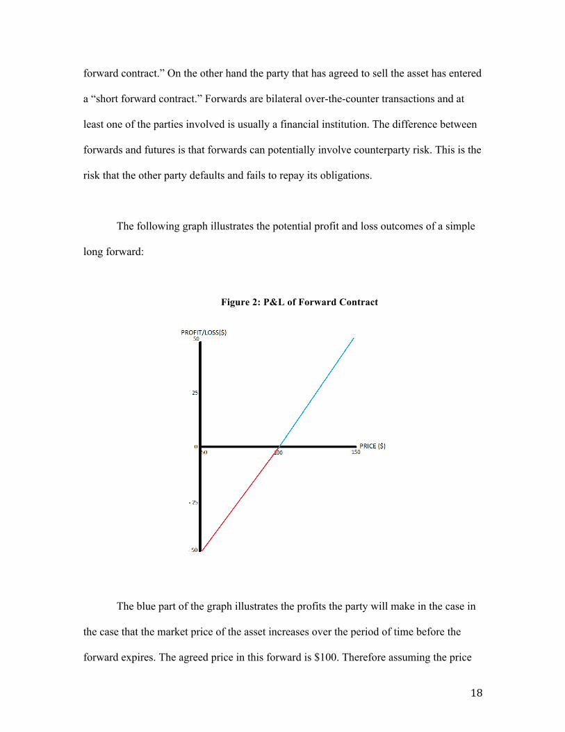
The following graph illustrates the potential profit and loss outcomes of a simple

long forward:

Figure 2: P&L of Forward Contract

The blue part of the graph illustrates the profits the party will make in the case in

the case that the market price of the asset increases over the period of time before the

forward expires. The agreed price in this forward is $100. Therefore assuming the price

19

of the asset reaches $150 the party in the long position can buy the asset for 100$ and sell

it back to the market for $150 thus getting a profit of 50$. On the other hand the red part

of the graph illustrates the loss in the case that the price of the asset falls below $100.

(The graph for a Short Forward would be the exact inverse of this graph)

An outright forward foreign exchange deal is:

- A binding commitment between two parties who agree to exchange two currencies at an

agreed rate on a future value date that is later than the spot date. By spot we mean the

usual two business days time a spot foreign exchange deal takes.

Outright forwards are used to a great extent by companies that make or receive payments

in foreign currencies. In the case they are receiving payments they will use an outright

forward to protect against a depreciation of their currency.

The forward FX rate is determined using the spot rate and the relative interest rate of the

two currencies. The determined rate has to be “fair” which implies that there potential

arbitrage opportunities need to be eliminated; otherwise one party would have a

comparative advantage over the other party. A cash-and-carry calculation is used to

calculate the fair rate. For instance, let us say a company is going to enter a long forward

for GBP/USD to be executed one year from today. The spot price at the time is 1.5

GBP/USD. Let’s assume that the US dollar interest rate is 3% p.a. (per annum) and the

Sterling interest rate is 5% p.a. This means a dollar can be invested at a rate of 3% in one

20

year and Sterling at a rate of 5%. Therefore 100 pounds invested today would equal 105

pounds in one year. On the other hand these 100 pounds equal 150 dollars, which if

invested today will grow into 154.5 dollars. So the value of a pound against a US dollar

in one year is calculated in the following way:

105 GBP = 154.5 USD 1 GBP = 154.5 / 105 USD 1 GBP = 1.4714 USD

Thus the theoretical annual forward rate is GBP/USD 1.4714.

Deliverable vs. Non-Deliverable Forwards

A Non-Deliverable Forward (NDF) is an outright forward contract in which the

counterparties settle the difference between the contracted NDF rate and the prevailing

spot rate on an agreed notional amount. It is used in various emerging markets where

forward FX trading has been banned by the government.

Spread

For every security in finance that is traded on a market, there is always a bid-offer spread.

It refers to the difference between the price quoted for a sale (the ask price) and a

purchase (the bid). The size of the spreads generally depends on the liquidity of the

market; in very liquid markets the spreads tend to be small and in illiquid ones the spread

is high. Due to its very high liquidity, the foreign exchange market has very tight spreads.

However, spreads vary within currency. For instance, the Euro typically has a spread of

0.0350%, while a less traded currency such as the Norwegian krone has a spread of

21

0.18%. When trading currencies, trading costs are usually associated with the spreads. In

our construction of the index later on this paper, the spreads are taking into consideration

when calculating total trading costs.

London Inter-Bank Offering Rate

In this paper, we will deal mainly with an index that uses the London Inter-Bank Offering

rate (Libor) as an indicator to either go long or short a currency. Each morning at 11am, a

group of banks known collectively as the British Bankers’ Association (BBA) gets

together and each participant sends its interbank borrowing rate. An average is calculated

using all the rates, and the process is done for every country’s Libor rate. Therefore,

Libor is the average interest rates that leading banks charge when lending to other banks.

Libor is an extremely important rate because it is used as a benchmark to trade an

immense amount of deals. It is used as a reference rate for many financial instruments

such as forward rate agreements, interest rate swaps, floating rate notes, currencies, just

to mention a few. The index that our MQP team built in RBS uses the Libor rate of each

country in the G10 as a measure to make investment decisions.

Volatility

Volatility is a crucial concept in finance and our index takes into account volatility in

order to make investment decisions. Volatility is a measure for the variation of price of a

financial instrument over time. It is commonly used to quantify the risk of the financial

instrument over a specific time period and is normally expressed in annualized terms.

22

Investors care about volatility for several reasons: first, the wider the swings in an

investment’s price the harder emotionally it is not to worry. Second, when certain cash

flows from selling a security are needed, higher volatility means a greater chance of a

shortfall. On the flipside, price volatility also presents opportunities to buy assets cheaply

and sell when overpriced. Volatility is usually calculated using the standard deviation

formula.

Matlab

Matlab is the main platform used to create our tool, which builds foreign exchange

indices. Matlab is a numerical computing environment and a fourth generation

programming language. It allows matrix manipulations, plotting of functions and data,

implementation of algorithms and creation of graphic user interfaces (GUI). Due to its

highly quantitative nature and numerical capabilities, Matlab has been well received by

the finance industry since Mathworks, the developer of Matlab, created a financial

toolbox.

23

3. Back test Modeling and Analysis of Dynamic FX Indices

3.1 Overall Project Idea

The FX Index business is highly dynamic. With the high growth of emerging

markets, the FX market is getting even larger demand new indices to trade. Since RBS is

only starting to get involved with FX indices, the indices being done are constructed on

Excel. Excel is an extremely useful tool in general and fantastic for many things but it has

been apparent that for complex indices that require many calculations and variables, it is

not ideal. In order to be more significant in the index business, RBS realized that they

need a new program to create them and have discovered that MATLAB would be a great

candidate, due to its high capability to deal with calculations in a short period of time.

Unfortunately, nobody in the Structuring team has had experience with MATLAB before

to start building indices right away. Our MQP program started in a very crucial time for

RBS since our project will consist of creating the MATLAB platform, and help the team

get started with this developing stage.

24

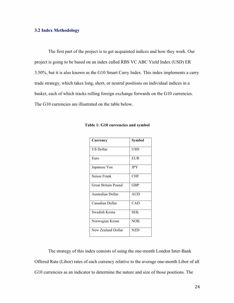
3.2 Index Methodology

The first part of the project is to get acquainted indices and how they work. Our

project is going to be based on an index called RBS VC ABC Yield Index (USD) ER

3.50%, but it is also known as the G10 Smart Carry Index. This index implements a carry

trade strategy, which takes long, short, or neutral positions on individual indices in a

basket, each of which tracks rolling foreign exchange forwards on the G10 currencies.

The G10 currencies are illustrated on the table below.

Table 1: G10 currencies and symbol

The strategy of this index consists of using the one-month London Inter-Bank

Offered Rate (Libor) rates of each currency relative to the average one-month Libor of all

G10 currencies as an indicator to determine the nature and size of those positions. The

Currency Symbol

US Dollar USD

Euro EUR

Japanese Yen JPY

Suisse Frank CHF

Great Britain Pound GBP

Australian Dollar AUD

Canadian Dollar CAD

Swedish Krona SEK

Norwegian Krone NOK

New Zealand Dollar NZD

25

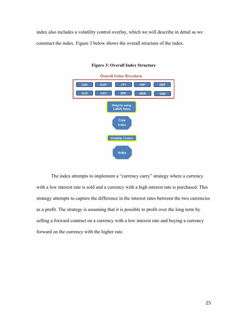
index also includes a volatility control overlay, which we will describe in detail as we

construct the index. Figure 3 below shows the overall structure of the index.

Figure 3: Overall Index Structure

The index attempts to implement a “currency carry” strategy where a currency

with a low interest rate is sold and a currency with a high interest rate is purchased. This

strategy attempts to capture the difference in the interest rates between the two currencies

as a profit. The strategy is assuming that it is possible to profit over the long term by

selling a forward contract on a currency with a low interest rate and buying a currency

forward on the currency with the higher rate.

26

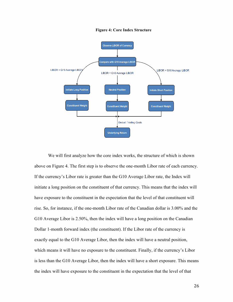
Figure 4: Core Index Structure

We will first analyze how the core index works, the structure of which is shown

above on Figure 4. The first step is to observe the one-month Libor rate of each currency.

If the currency’s Libor rate is greater than the G10 Average Libor rate, the Index will

initiate a long position on the constituent of that currency. This means that the index will

have exposure to the constituent in the expectation that the level of that constituent will

rise. So, for instance, if the one-month Libor rate of the Canadian dollar is 3.00% and the

G10 Average Libor is 2.50%, then the index will have a long position on the Canadian

Dollar 1-month forward index (the constituent). If the Libor rate of the currency is

exactly equal to the G10 Average Libor, then the index will have a neutral position,

which means it will have no exposure to the constituent. Finally, if the currency’s Libor

is less than the G10 Average Libor, then the index will have a short exposure. This means

the index will have exposure to the constituent in the expectation that the level of that

27

constituent will fall. The next step is to determine the size of those positions, which is

expressed as the “Weight”. How large the position will be depends on the absolute value

of the difference between the Libor rate of the currency and the G10 Average Libor. For

instance, if the difference between the GBP Libor and the average is 1.20 basis points,

and the difference between CAD Libor and the average is 1.40 basis points, then the

index will have a larger position on CAD than GBP. The next step needed to calculate the

Core Index is to use those weights of each individual currency to yield the Underlying

Return. A trading cost, which is incurred each time the index enters a new position, is

applied to the Underlying Return and ultimately the Core Index Level is calculated.

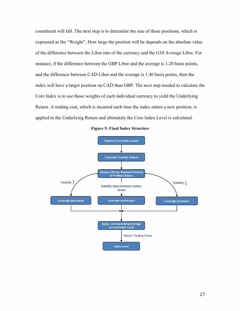
Figure 5: Final Index Structure

28

Now that we have discussed how the Core Index is calculated, we will now

describe how to get the final Index, which includes a volatility control component. The

final index is shown on the illustration above. The first step is to observe the Core Index

levels, in order to calculate the Portfolio Return. After calculating the Portfolio Return,

the next step is to observe the 20-day realized volatility of the portfolio return. This is

calculated by using the standard deviation and will be described with greater detail on a

next section. After calculating the 20-day realized volatility we will have, similarly to the

Core Index, three scenarios. If the volatility increases to certain levels, the leverage of the

index will be decreased. If the volatility stays between certain levels, in other words it

does not go up or down significantly, then the leverage of the index will stay unchanged.

Finally, if the volatility decreases to certain levels, the leverage will be increased. After

determining the amount of leverage of the index, we will apply it to the Core Index level.

Finally, we will deduct trading costs, which take place each time the leverage is

modified. This will give us the final Index Level.

29

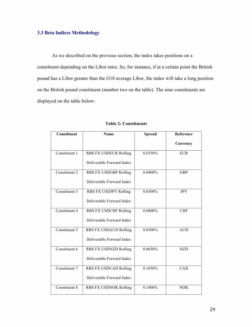
3.3 Beta Indices Methodology

As we described on the previous section, the index takes positions on a

constituent depending on the Libor rates. So, for instance, if at a certain point the British

pound has a Libor greater than the G10 average Libor, the index will take a long position

on the British pound constituent (number two on the table). The nine constituents are

displayed on the table below:

Table 2: Constituents

Constituent Name Spread Reference

Currency

Constituent 1 RBS FX USDEUR Rolling

Deliverable Forward Index

0.0350% EUR

Constituent 2 RBS FX USDGBP Rolling

Deliverable Forward Index

0.0400% GBP

Constituent 3 RBS FX USDJPY Rolling

Deliverable Forward Index

0.0300% JPY

Constituent 4 RBS FX USDCHF Rolling

Deliverable Forward Index

0.0800% CHF

Constituent 5 RBS FX USDAUD Rolling

Deliverable Forward Index

0.0500% AUD

Constituent 6 RBS FX USDNZD Rolling

Deliverable Forward Index

0.0650% NZD

Constituent 7 RBS FX USDCAD Rolling

Deliverable Forward Index

0.1050% CAD

Constituent 8 RBS FX USDNOK Rolling 0.1800% NOK

30

Deliverable Forward Index

Constituent 9 RBS FX USDSEK Rolling

Deliverable Forward Index

0.0600% SEK

These constituents are all indices, which serve as the base of the Core Index. Each

one of these indices is a Rolling Deliverable Forward of the USD against the specified

currency. The level of the rolling deliverable forward indices rises, falls, or stays the

same based on outright forward rates and spot exchange rates. For example, if the

outright forward rate on the current rebalancing date for exchanging USD with the

specified currency is greater than the spot rate on the next rebalancing date, then the

constituent will be higher. Each index is composed of deliverable foreign exchange

contracts in respect of a currency pair that notionally sells a fixed amount of US dollars

against the future purchase of a different reference currency (for instance, EUR). The

contracts are rolled on a monthly basis, which means that, since each contract lasts 1

month, a new contract is bought at a given date each month. It is a convention that this

rolling date is on each 20th of the month.

On each calculation date, the level of the index will be equal to the sum of:

1) The profit or loss that would be realized on the next roll date in respect of the

contract determined by reference to the Forward Rates on such calculation date

and

31

2) The index level on the immediately preceding roll date. On the next roll date,

the forward rate will be compared to the prevailing spot fixing rate fr the

currency pair to determine whether a profit or loss has been made.

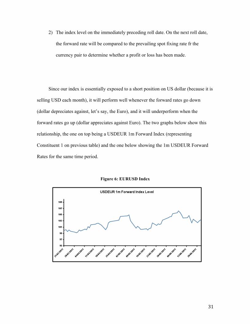
Since our index is essentially exposed to a short position on US dollar (because it is

selling USD each month), it will perform well whenever the forward rates go down

(dollar depreciates against, let’s say, the Euro), and it will underperform when the

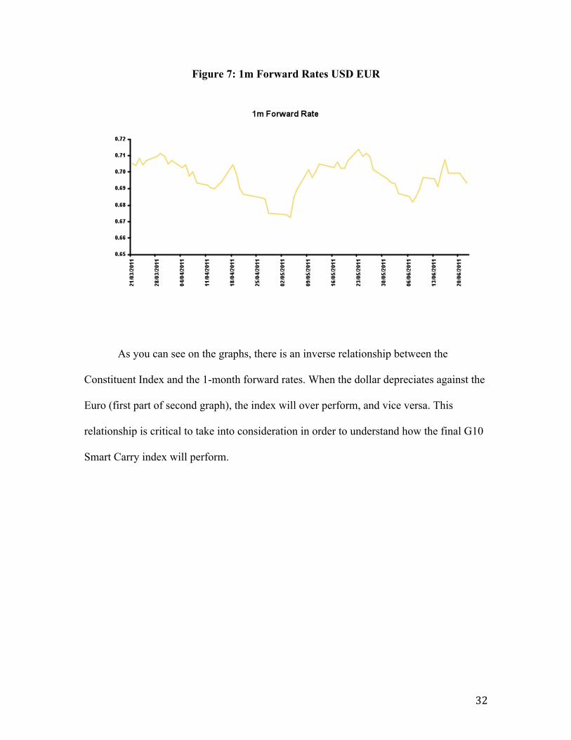
forward rates go up (dollar appreciates against Euro). The two graphs below show this

relationship, the one on top being a USDEUR 1m Forward Index (representing

Constituent 1 on previous table) and the one below showing the 1m USDEUR Forward

Rates for the same time period.

Figure 6: EURUSD Index

32

Figure 7: 1m Forward Rates USD EUR

As you can see on the graphs, there is an inverse relationship between the

Constituent Index and the 1-month forward rates. When the dollar depreciates against the

Euro (first part of second graph), the index will over perform, and vice versa. This

relationship is critical to take into consideration in order to understand how the final G10

Smart Carry index will perform.

33

Excel Construction

Now that we have described how the constituents work, we will now provide an

explanation of how the final index is constructed in Excel. Essentially, as we mentioned

before, nine Constituent levels will be used, each representing the currency pairs of the

G10: USDEUR, USDJPY, USDCHF, USDGBP, USDAUD, USDCAD, USDSEK,

USDNOK. In reality, we don’t have to manually compute the index levels of all of these

nine pairs, they are already given and are published in Bloomberg. As outlined

previously, the Core Index is constructed first and then the volatility control component is

added to have the final Index.

1) The first step to create any index is to get the correct calculation dates. The

index will be back tested from the 20th of January 2000 to August 11th 2011. Of

that period, only combined days where currency markets in all countries are open

will be included in the calculation. This task is not as straightforward as it seems.

To get the right dates, the first step is to find the business days of each of the ten

currencies. After we make this list with 10 columns, the next step is to find the

business days, which all the ten currencies share. In other words, for example on

the 4th of July, nine of the G10 countries might have their markets open but the

US doesn’t. Therefore, the 4th of July would not be included in our index. This

process has to be done over a 10-year period, calculating each single day. Excel

can do this by doing an if function.

34

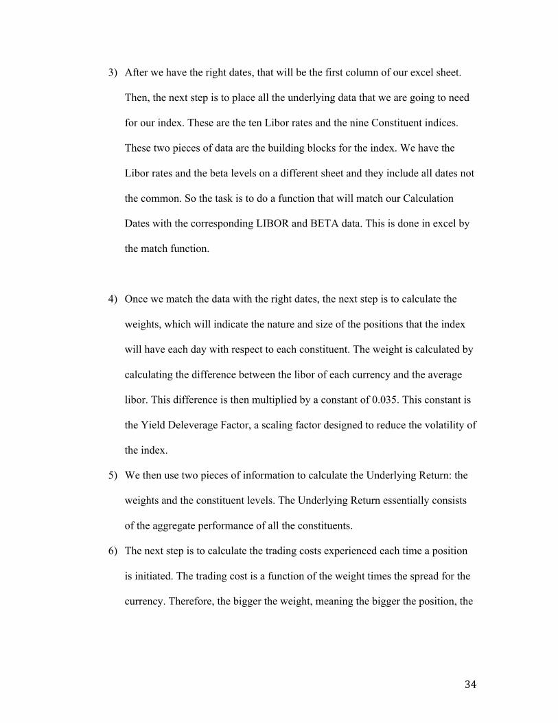
3) After we have the right dates, that will be the first column of our excel sheet.

Then, the next step is to place all the underlying data that we are going to need

for our index. These are the ten Libor rates and the nine Constituent indices.

These two pieces of data are the building blocks for the index. We have the

Libor rates and the beta levels on a different sheet and they include all dates not

the common. So the task is to do a function that will match our Calculation

Dates with the corresponding LIBOR and BETA data. This is done in excel by

the match function.

4) Once we match the data with the right dates, the next step is to calculate the

weights, which will indicate the nature and size of the positions that the index

will have each day with respect to each constituent. The weight is calculated by

calculating the difference between the libor of each currency and the average

libor. This difference is then multiplied by a constant of 0.035. This constant is

the Yield Deleverage Factor, a scaling factor designed to reduce the volatility of

the index.

5) We then use two pieces of information to calculate the Underlying Return: the

weights and the constituent levels. The Underlying Return essentially consists

of the aggregate performance of all the constituents.

6) The next step is to calculate the trading costs experienced each time a position

is initiated. The trading cost is a function of the weight times the spread for the

currency. Therefore, the bigger the weight, meaning the bigger the position, the

35

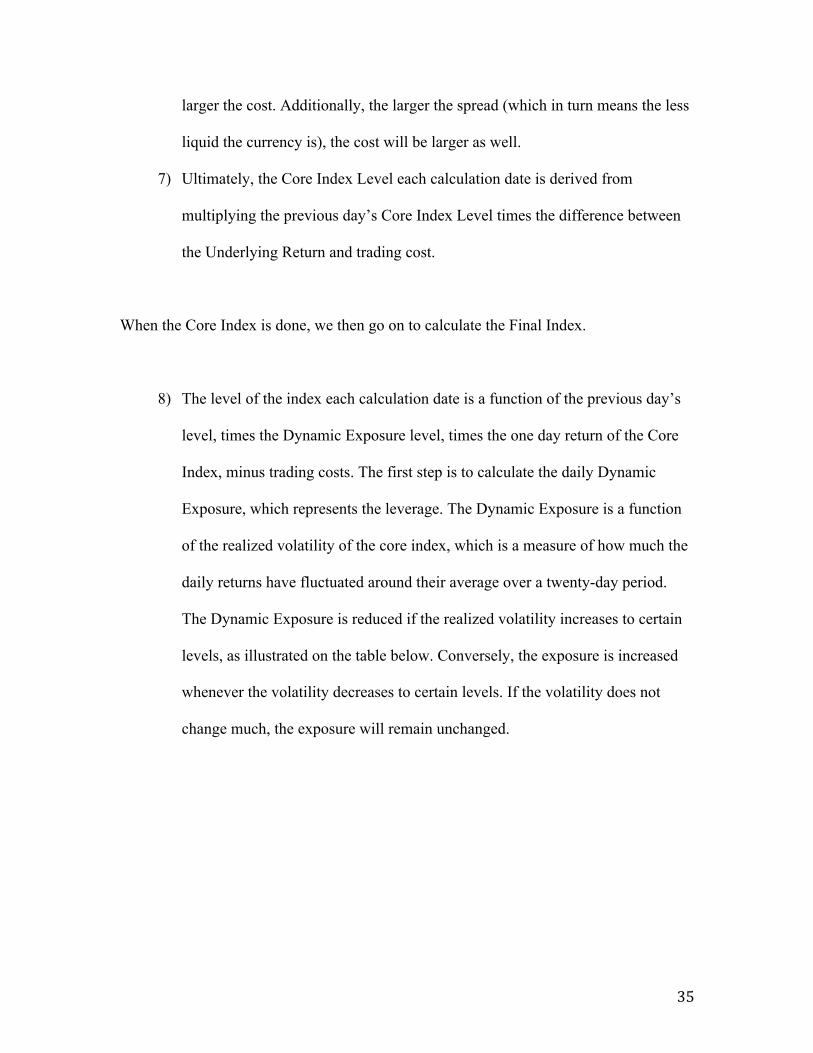
larger the cost. Additionally, the larger the spread (which in turn means the less

liquid the currency is), the cost will be larger as well.

7) Ultimately, the Core Index Level each calculation date is derived from

multiplying the previous day’s Core Index Level times the difference between

the Underlying Return and trading cost.

When the Core Index is done, we then go on to calculate the Final Index.

8) The level of the index each calculation date is a function of the previous day’s

level, times the Dynamic Exposure level, times the one day return of the Core

Index, minus trading costs. The first step is to calculate the daily Dynamic

Exposure, which represents the leverage. The Dynamic Exposure is a function

of the realized volatility of the core index, which is a measure of how much the

daily returns have fluctuated around their average over a twenty-day period.

The Dynamic Exposure is reduced if the realized volatility increases to certain

levels, as illustrated on the table below. Conversely, the exposure is increased

whenever the volatility decreases to certain levels. If the volatility does not

change much, the exposure will remain unchanged.

36

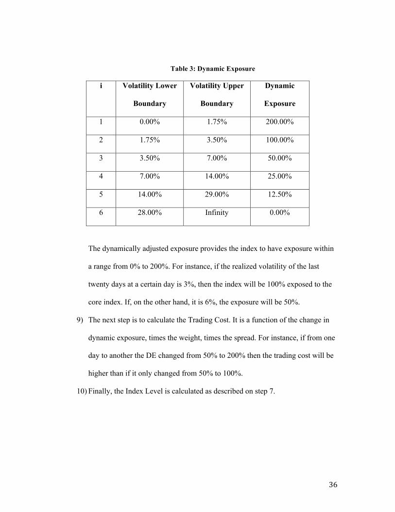
Table 3: Dynamic Exposure

i Volatility Lower

Boundary

Volatility Upper

Boundary

Dynamic

Exposure

1 0.00% 1.75% 200.00%

2 1.75% 3.50% 100.00%

3 3.50% 7.00% 50.00%

4 7.00% 14.00% 25.00%

5 14.00% 29.00% 12.50%

6 28.00% Infinity 0.00%

The dynamically adjusted exposure provides the index to have exposure within

a range from 0% to 200%. For instance, if the realized volatility of the last

twenty days at a certain day is 3%, then the index will be 100% exposed to the

core index. If, on the other hand, it is 6%, the exposure will be 50%.

9) The next step is to calculate the Trading Cost. It is a function of the change in

dynamic exposure, times the weight, times the spread. For instance, if from one

day to another the DE changed from 50% to 200% then the trading cost will be

higher than if it only changed from 50% to 100%.

10) Finally, the Index Level is calculated as described on step 7.

37

Construction of Index in Matlab

Now that we have made the index in Excel, we will start creating the Matlab tool.

MATLAB is a high level language and interactive environment that enables you to

perform computationally extensive tasks faster than with traditional programming

languages such as C, C++, and Fortran. It is a highly quantitative language, which proves

to be extremely useful in the financial world. What makes Matlab so efficient is that it

has many commands that allow us to achieve in one step what Excel would achieve in

three or four. It makes construction easier and simpler. We will first walk through the

process of construction the G10 Smart Carry Index in Matlab and afterwards we will

provide specific examples where Matlab’s efficiency and time savings compares to

Excel.

The beauty of Matlab is that we can build this highly technical index look like a

document with instructions. In essence, our objective is to make our code look like the

legal document we talked about earlier. That way, anyone who wants to read our code

will understand it and know what is going on. This will allow that person to make

changes easily to the code in order to create variations of the index. In order to be able to

better visualize what the end code should look like it was essential to get acquainted with

the implementation of the index through Matlab. This is why our first steps in this project

using the Matlab software were:

‐ Inputting all the data needed to calculate the index into Matlab matrixes.

38

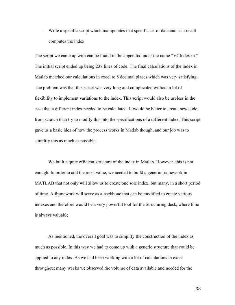
‐ Write a specific script which manipulates that specific set of data and as a result

computes the index.

The script we came up with can be found in the appendix under the name “VCIndex.m.”

The initial script ended up being 238 lines of code. The final calculations of the index in

Matlab matched our calculations in excel to 8 decimal places which was very satisfying.

The problem was that this script was very long and complicated without a lot of

flexibility to implement variations to the index. This script would also be useless in the

case that a different index needed to be calculated. It would be better to create new code

from scratch than try to modify this into the specifications of a different index. This script

gave us a basic idea of how the process works in Matlab though, and our job was to

simplify this as much as possible.

We built a quite efficient structure of the index in Matlab. However, this is not

enough. In order to add the most value, we needed to build a generic framework in

MATLAB that not only will allow us to create one sole index, but many, in a short period

of time. A framework will serve as a backbone that can be modified to create various

indexes and therefore would be a very powerful tool for the Structuring desk, where time

is always valuable.

As mentioned, the overall goal was to simplify the construction of the index as

much as possible. In this way we had to come up with a generic structure that could be

applied to any index. As we had been working with a lot of calculations in excel

throughout many weeks we observed the volume of data available and needed for the

39

computations. All of this data was interrelated somehow. As mentioned before a lot of the

information was referenced through a Vlookup, which returned a value corresponding to

a specific date. We realized the dates were the point of connection between the vast

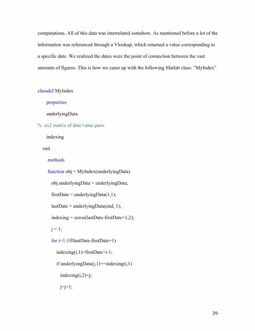
amounts of figures. This is how we came up with the following Matlab class: “MyIndex”

classdef MyIndex

properties

underlyingData

% nx2 matrix of date/value pairs

indexing

end

methods

function obj = MyIndex(underlyingData)

obj.underlyingData = underlyingData;

firstDate = underlyingData(1,1);

lastDate = underlyingData(end, 1);

indexing = zeros(lastDate-firstDate+1,2);

j = 1;

for i=1:1lastDate-firstDate+1)

indexing(i,1)=firstDate+i-1;

if underlyingData(j,1)==indexing(i,1)

indexing(i,2)=j;

j=j+1;

40

else

indexing(i,2)=-1;

end

end

obj.indexing = indexing;

end

end

This class can actually be used for any type of data organized according to a date series.

This is explained with an example:

Let’s assume we create an object for the Core Index with the class MyIndex. Let’s name

it coreIndex.

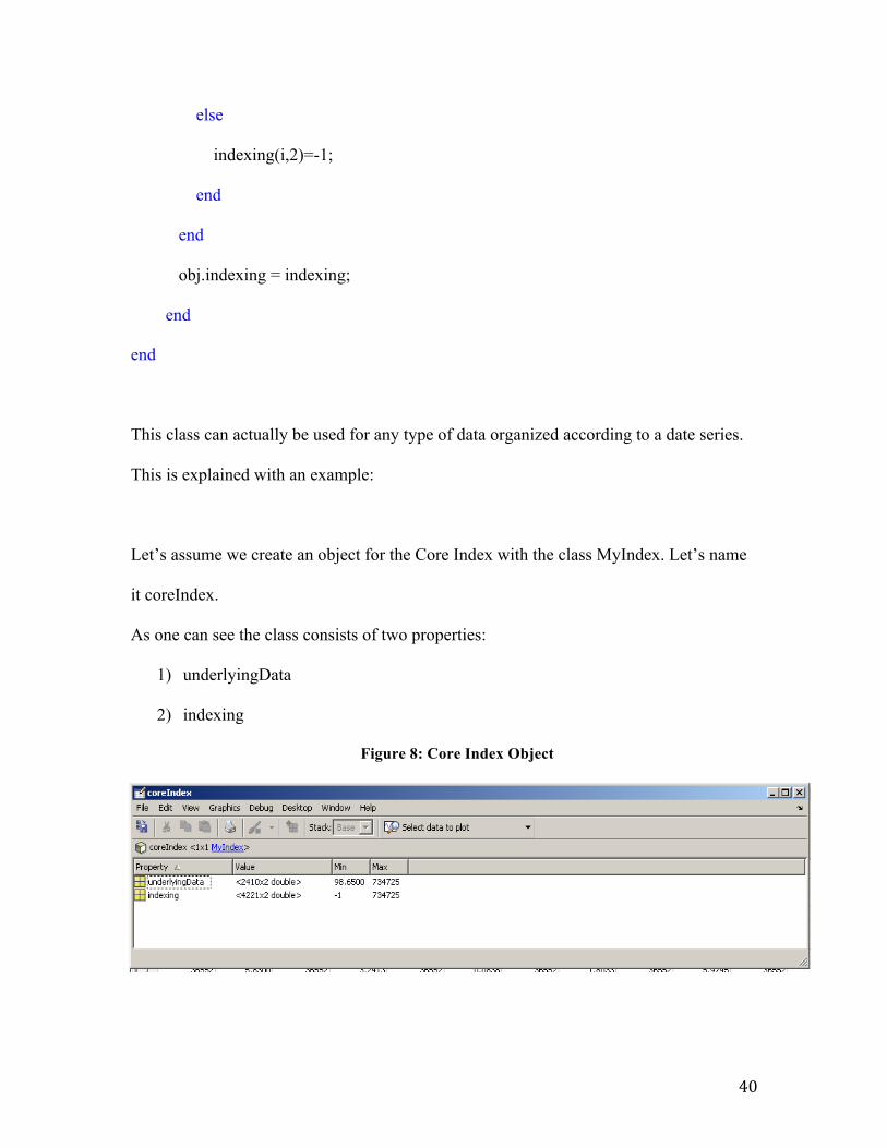
As one can see the class consists of two properties:

1) underlyingData

2) indexing

Figure 8: Core Index Object

41

Both of them are nX2 matrixes meaning they consist of two columns and any number

of rows.

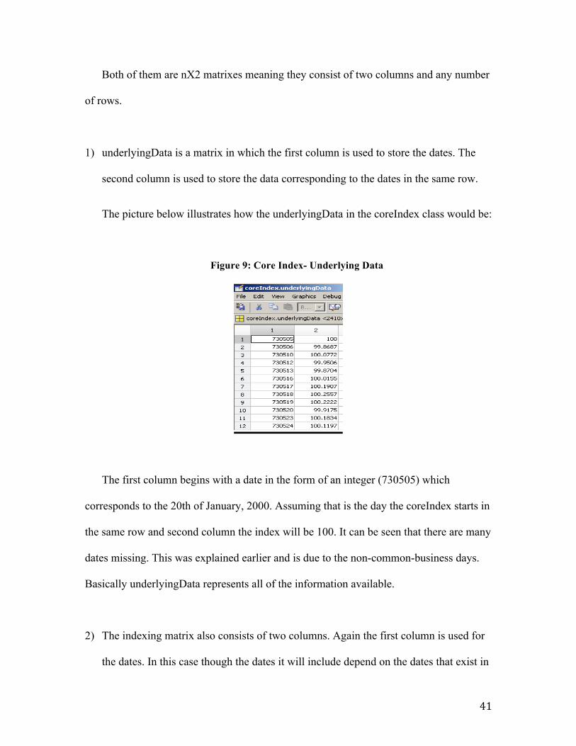
1) underlyingData is a matrix in which the first column is used to store the dates. The

second column is used to store the data corresponding to the dates in the same row.

The picture below illustrates how the underlyingData in the coreIndex class would be:

Figure 9: Core Index- Underlying Data

The first column begins with a date in the form of an integer (730505) which

corresponds to the 20th of January, 2000. Assuming that is the day the coreIndex starts in

the same row and second column the index will be 100. It can be seen that there are many

dates missing. This was explained earlier and is due to the non-common-business days.

Basically underlyingData represents all of the information available.

2) The indexing matrix also consists of two columns. Again the first column is used for

the dates. In this case though the dates it will include depend on the dates that exist in

42

the underlyingData matrix. The dates in the first column are all the actual dates from

the start date to the last date in the underlyingData matrix, but no days in between

those two dates are excluded. This means that every single date in between those two

days will appear in the first column of the matrix.

This is calculated through an algorithm every time a new variable is defined as

MyIndex. The second column consists of a list of integers. These integers represent the

vertical position/index of the specific date (of the first column) in the underlyingData,

thus the name of the property “indexing.” An indexing of 2 means that that date is in the

second row of the underlyingData. This is done in the code by checking every date in the

indexing matrix one by one. The first date gets an indexing value of 1; because the start

date is located in the first row of the underlyingData as it is the first date in which we

have data. Every date in the indexing matrix is checked and matched to the same date in

the underlyingData.

As mentioned above while the indexing matrix includes all possible dates between the

start date and the end date, the underlyingData excludes bank holidays and non-common

business days. If a date does not exist in the underlyingData (holidays excluded) its

indexing value will be -1. In this way we flag that that date does not appear in our data.

The next date that actually exists in both matrixes will take the indexing value of its

position in the underlyingData matrix. This is done by going back to the previous date

that exists in both matrixes, get its indexing value, and add 1.

43

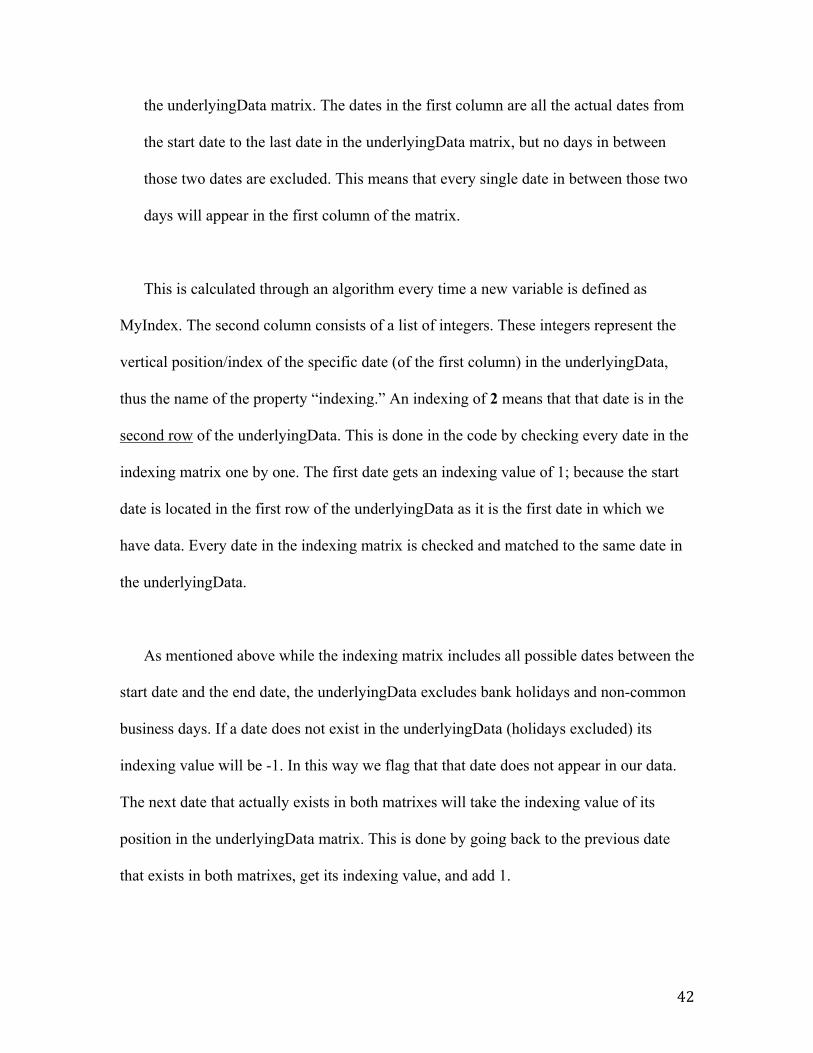
The indexing matrix basically serves as a mapping of the position of the dates in the

underlyingData. Essentially, underlyingData is more like a database of information

while indexing is used as a tool to manage the database.

In order to illustrate this let’s take a look at both properties side by side:

Figure 10: Matrices

44

Let’s take two examples. Date 730507 is not part of the underlyingData. This is

why it has an indexing of 1. The next date that exists in underlyingData is 730510. Its

indexing/position was calculated by taking the date 730506; which is the previous

common date; get its indexing (position = 2) and add 1. Thus the indexing/position of

date 730510 is 2+1=3. As we can see that date appears in the 3rd row.

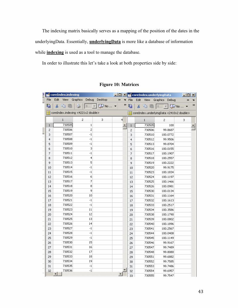
This indexing matrix allowed us to be able to create functions like the valueAt(t)

function which would take as an input a date and return the value corresponding to that

date. For example in the case of the coreIndex variable demonstrated above the value of

the index corresponding to the date 730510 is 100.0772. So we wanted to be able to write

valueAt(730510) and get 100.0772.This function could be done in many ways. One way

would be searching all through the matrix until the required date was found. Searching

though required complex algorithms that result in high time lag, especially in the case of

the calculation of an index with a data history of decades. There is so much data, that

searching is just inefficient, so we utilized our structure to create a function where no

searching needs to take place.

Figure 11: Indexing Matrix

45

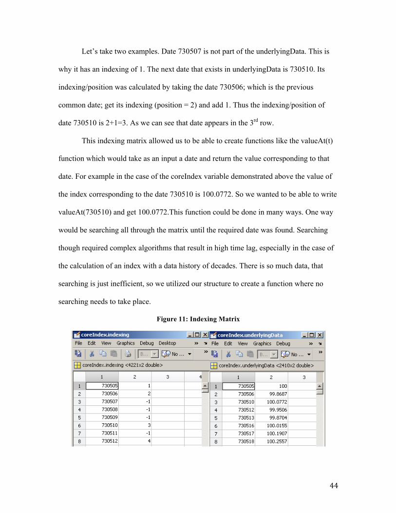
Let’s take a look at the code of the function valueAt:

function val = valueAt(obj, t)

val = obj.underlyingData(obj.indexing(t - obj.indexing(1,1)+1,2), 2);

end

Let’s see again how this works step by step. Let’s take this example:

coreIndex.valueAt(730510)

The date inputted is 730510. In order to get the data corresponding to that date we need to

have that date’s indexing (which is 3), go to the underlyingData to the 3rd row and 2nd

column and we got the value at that date. In order to comprehend the code it’s easier to

break it into parts from the inside to the outside.

t-obj.indexing(1,1)+1,2

t = 730510 (the date inputted)

obj.indexing(1,1) = 730505 (start date)

If you subtract the start date from the inputted date and add 1 you basically get the

position of the inputted date in the indexing matrix: 730510 – 730505 + 1 = 6. If you take

a look in the indexing matrix in the image above one can see this is indeed the case.

46

Figure 12: Index positioning

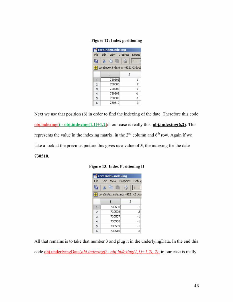
Next we use that position (6) in order to find the indexing of the date. Therefore this code

obj.indexing(t - obj.indexing(1,1)+1,2)in our case is really this: obj.indexing(6,2). This

represents the value in the indexing matrix, in the 2nd column and 6th row. Again if we

take a look at the previous picture this gives us a value of 3, the indexing for the date

730510.

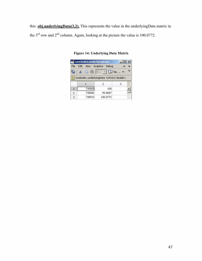
Figure 13: Index Positioning II

All that remains is to take that number 3 and plug it in the underlyingData. In the end this

code obj.underlyingData(obj.indexing(t - obj.indexing(1,1)+1,2), 2); in our case is really

47

this: obj.underlyingData(3,2). This represents the value in the underlyingData matrix in

the 3rd row and 2nd column. Again, looking at the picture the value is 100.0772.

Figure 14: Underlying Data Matrix

48

Excel vs. the MATLAB tool

We can explain the difference between Excel and Matlab by using a maze as a

symbol. Excel is like a person in a maze, it will enter it, do a lot of loops and go back and

forward repetitively, but it will manage to get out eventually. Matlab, on the other hand,

is a person with a jetpack who flies over the maze, looking at it from a perspective from

above, and navigating through it to the finish. At the end of the day, both arrive to the end

of the maze, but one does it much faster and “cleaner” than the other. Excel is indeed a

great tool; it offers relatively high calculation speed. However, it offers a micro point of

view. It doesn’t “see” the whole picture, the maze. When creating a complex structure

such as a financial index, a micro point of view makes it harder for the user to minimize

mistakes and in general will be more confusing to navigate. Matlab is a high-performance

programming language that uses vectors and matrices as basic building blocks. Instead of

dealing with individual cells, like Excel does, Matlab deals with chunks, or blocks of data

and moves them around. It offers a macro point of view. It allows users to see data with a

bigger perspective and to spot mistakes in the structure. Matlab allows this by providing

helper functions, which are tested and have predictable behavior. Its data representation is

very clean with the ability to assign variables for any set of data. Ultimately, this will lead

to greater reliability for the final result. We will discuss one of the many instances in

building an index where Matlab provides to be a more efficient program in Excel: the

process of calculating the G10 Libor average.

49

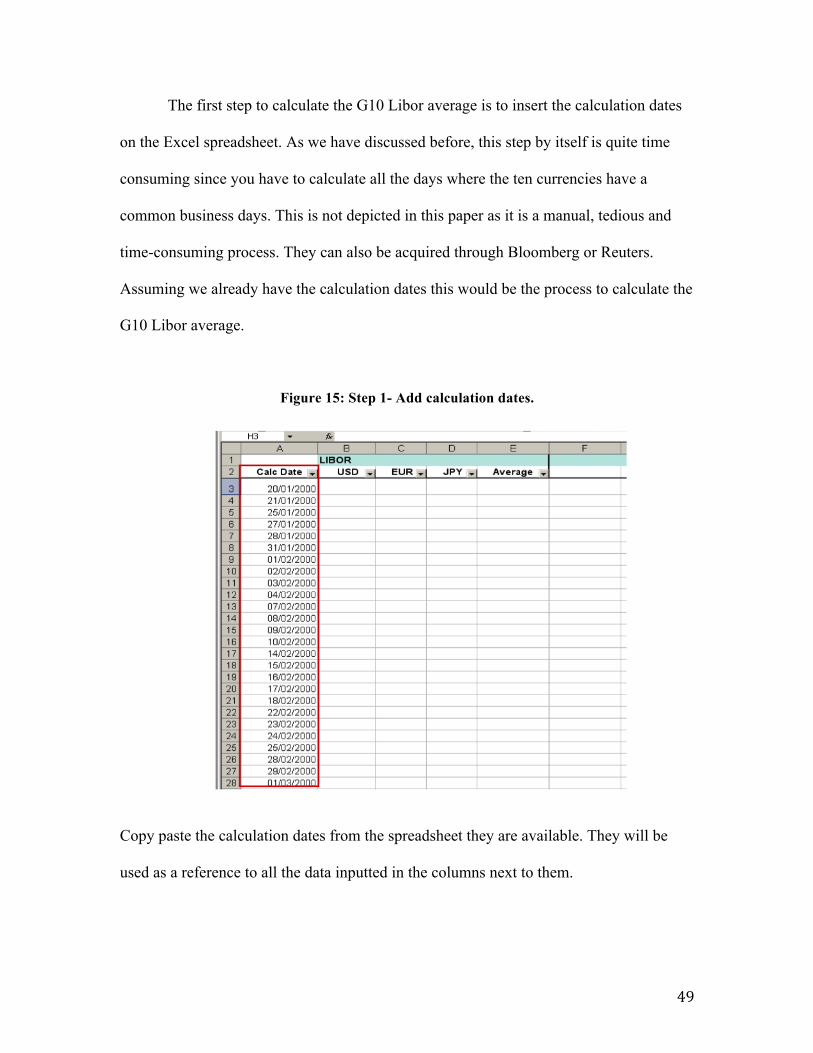
The first step to calculate the G10 Libor average is to insert the calculation dates

on the Excel spreadsheet. As we have discussed before, this step by itself is quite time

consuming since you have to calculate all the days where the ten currencies have a

common business days. This is not depicted in this paper as it is a manual, tedious and

time-consuming process. They can also be acquired through Bloomberg or Reuters.

Assuming we already have the calculation dates this would be the process to calculate the

G10 Libor average.

Figure 15: Step 1- Add calculation dates.

Copy paste the calculation dates from the spreadsheet they are available. They will be

used as a reference to all the data inputted in the columns next to them.

50

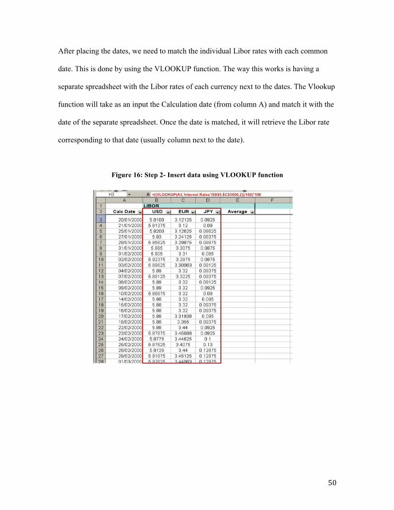
After placing the dates, we need to match the individual Libor rates with each common

date. This is done by using the VLOOKUP function. The way this works is having a

separate spreadsheet with the Libor rates of each currency next to the dates. The Vlookup

function will take as an input the Calculation date (from column A) and match it with the

date of the separate spreadsheet. Once the date is matched, it will retrieve the Libor rate

corresponding to that date (usually column next to the date).

Figure 16: Step 2- Insert data using VLOOKUP function

51

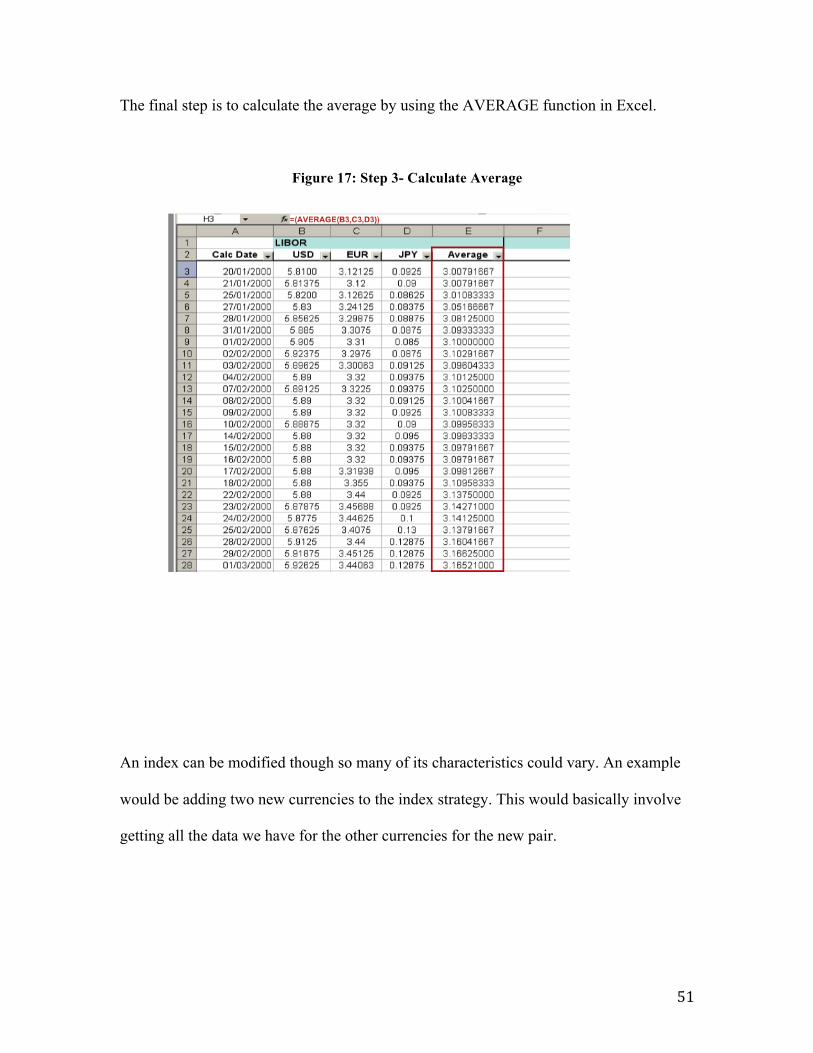
The final step is to calculate the average by using the AVERAGE function in Excel.

Figure 17: Step 3- Calculate Average

An index can be modified though so many of its characteristics could vary. An example

would be adding two new currencies to the index strategy. This would basically involve

getting all the data we have for the other currencies for the new pair.

52

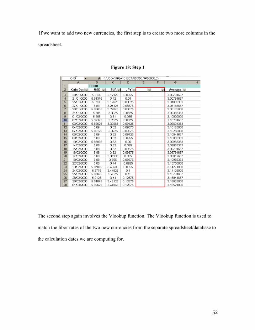
If we want to add two new currencies, the first step is to create two more columns in the

spreadsheet.

Figure 18: Step 1

The second step again involves the Vlookup function. The Vlookup function is used to

match the libor rates of the two new currencies from the separate spreadsheet/database to

the calculation dates we are computing for.

53

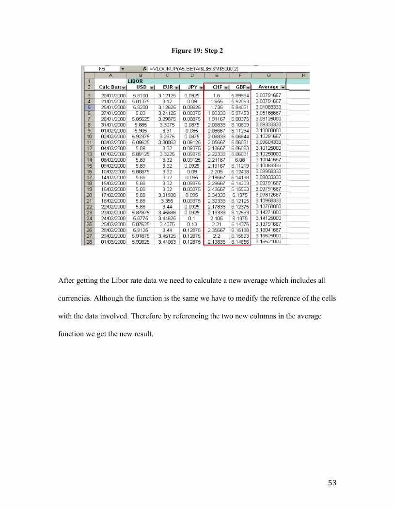
Figure 19: Step 2

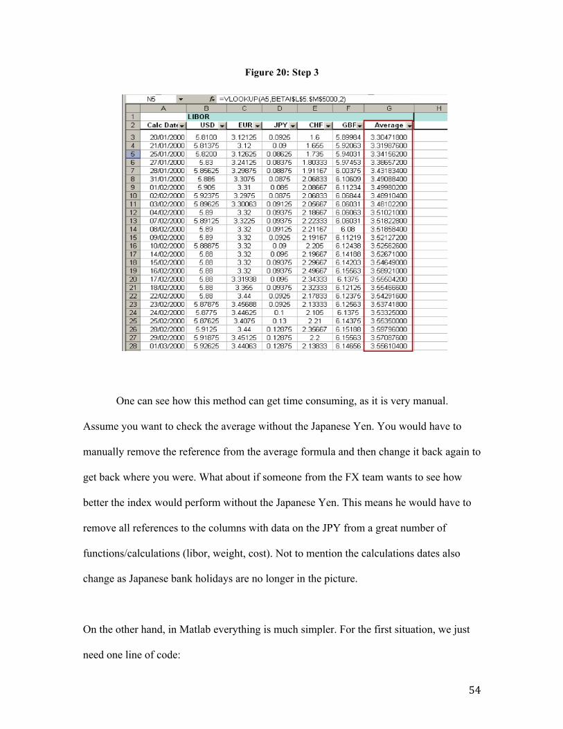
After getting the Libor rate data we need to calculate a new average which includes all

currencies. Although the function is the same we have to modify the reference of the cells

with the data involved. Therefore by referencing the two new columns in the average

function we get the new result.

54

Figure 20: Step 3

One can see how this method can get time consuming, as it is very manual.

Assume you want to check the average without the Japanese Yen. You would have to

manually remove the reference from the average formula and then change it back again to

get back where you were. What about if someone from the FX team wants to see how

better the index would perform without the Japanese Yen. This means he would have to

remove all references to the columns with data on the JPY from a great number of

functions/calculations (libor, weight, cost). Not to mention the calculations dates also

change as Japanese bank holidays are no longer in the picture.

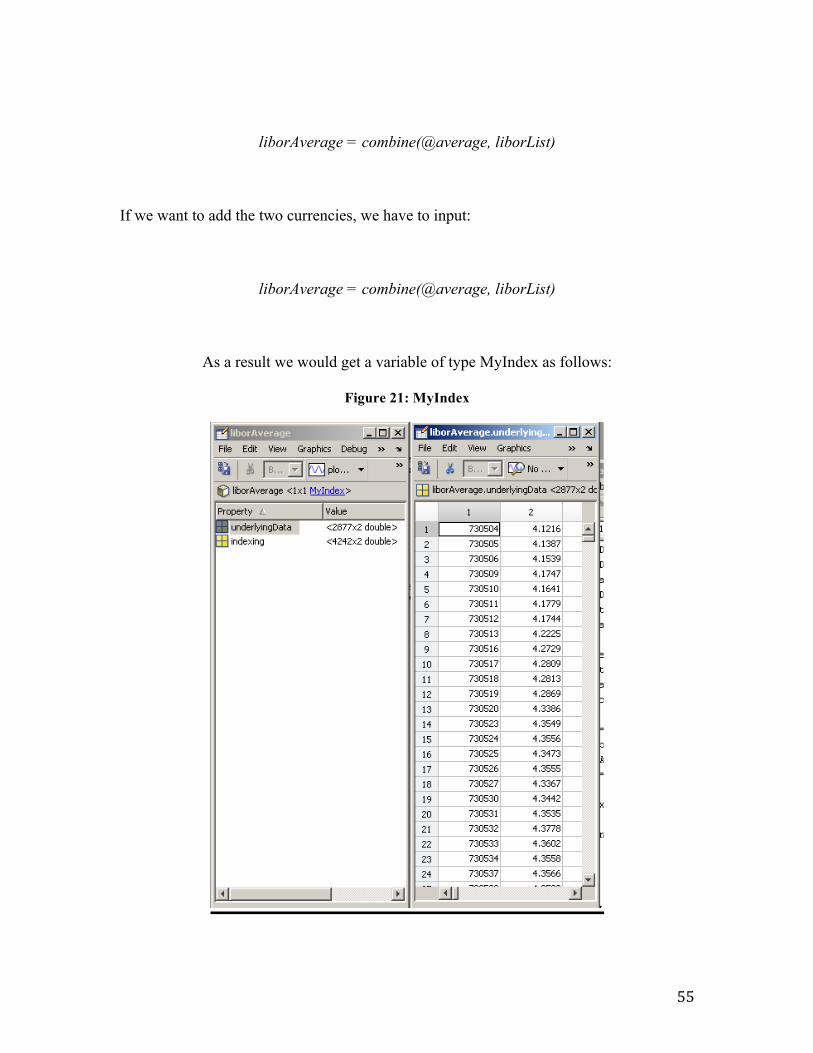
On the other hand, in Matlab everything is much simpler. For the first situation, we just

need one line of code:

55

liborAverage = combine(@average, liborList)

If we want to add the two currencies, we have to input:

liborAverage = combine(@average, liborList)

As a result we would get a variable of type MyIndex as follows:

Figure 21: MyIndex

56

The code stays the same and gives us the same result as the liborList will

automatically be generated according to the data available. No modification needs to be

made to the process. The only factor that changes here is the data available. So in the

case you were to add two new currencies to the database from which the code is getting

its records, the liborList would automatically include all the information of the two new

currencies as well.

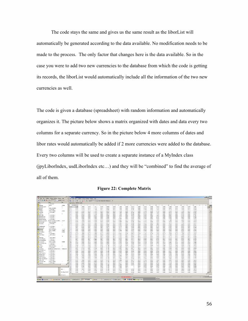
The code is given a database (spreadsheet) with random information and automatically

organizes it. The picture below shows a matrix organized with dates and data every two

columns for a separate currency. So in the picture below 4 more columns of dates and

libor rates would automatically be added if 2 more currencies were added to the database.

Every two columns will be used to create a separate instance of a MyIndex class

(jpyLiborIndex, usdLiborIndex etc…) and they will be “combined” to find the average of

all of them.

Figure 22: Complete Matrix

57

Unfortunately due to compliance reasons we are not able to include all our functions,

scripts and code.

58

Matlab Tool and Variations

One of the most important benefits of Matlab is that the code is highly versatile. It is very

easy and it takes little time to make any necessary amendments to the index. Foreign

exchange markets are constantly changing and so are the needs of a bank’s clients.

Therefore, having a versatile index that allows the structuring team to modify its index in

order to satisfy changes in their clients needs is a great plus. In this section we will

discuss two examples of index modifications and how Matlab can be beneficial.

As you know, the index is a carry trade strategy, which uses actual one-month Libor rates

of each currency relative to the average one-month Libor of all G10 currencies as an

indicator to determine the nature and size of those positions. However, it is a possibility

that using actual Libor rates might not be ideal and instead using implied Libor rates

might provide better returns. Implied rates are calculated by inputting the spot rate,

forward rate, and actual interest rate. We will provide an example using EURUSD to

illustrate the difference between actual and implied rates.

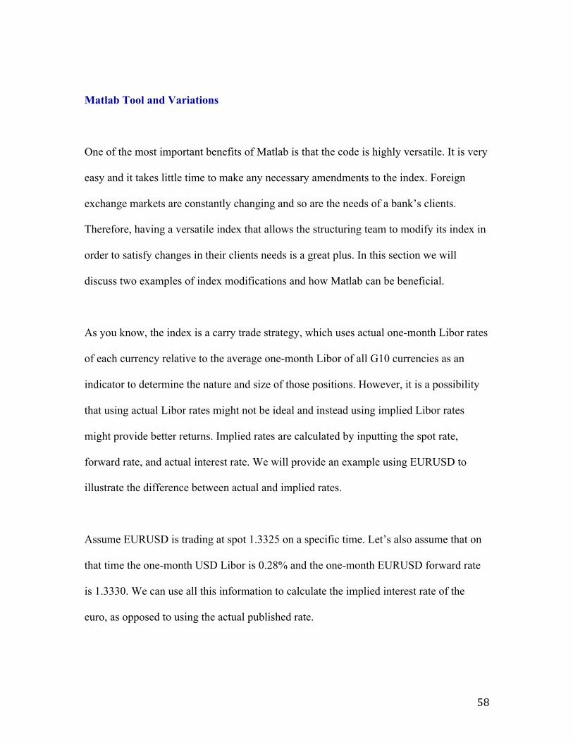
Assume EURUSD is trading at spot 1.3325 on a specific time. Let’s also assume that on

that time the one-month USD Libor is 0.28% and the one-month EURUSD forward rate

is 1.3330. We can use all this information to calculate the implied interest rate of the

euro, as opposed to using the actual published rate.

59

Figure 23: Diagram of implied rate calculation

We start on the top left rectangle, and we will assume that we have one million

Euros. The first step is to exchange the Euros for US dollars. With a spot rate of 1.3325,

we will have $1,332,500. The next step is to “invest” that US dollar amount for one

month, using the 1-month Libor rate. This will yield $1,332,811. Subsequently, we will

apply the 1-month forward exchange rate to get Euros. Dividing $1,332,811 by 1.3330

will give us EUR 999,858. This figure is less than the initial 1 million EUR, which means

there is a negative interest rate. Therefore, the implied interest rate must be negative.

Indeed this is the case and if we do a simple calculation the implied interest rates comes

out to -0.17%. This is substantially different to the actual rate, which is 1.32%. The

difference, 149 bps, which is also known as the basis, is significant. Clearly, using

implied rates for our trading strategy as opposed to actual rates will give us different

60

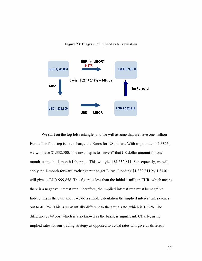
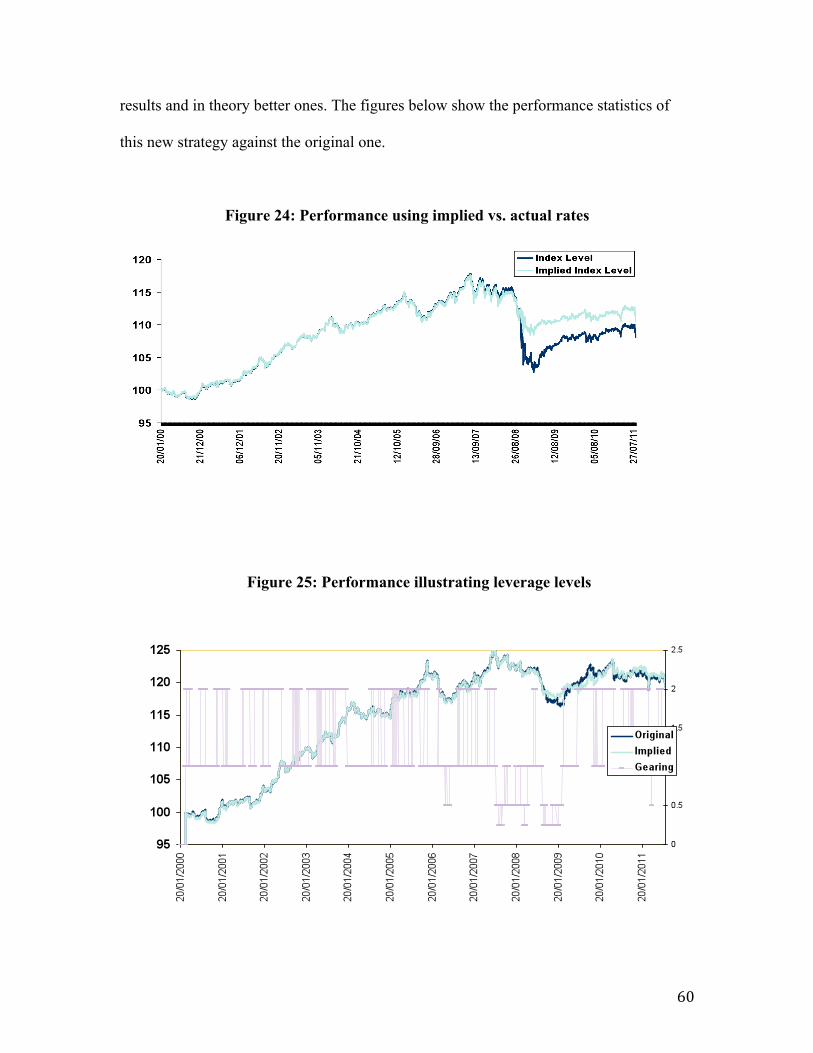
results and in theory better ones. The figures below show the performance statistics of

this new strategy against the original one.

Figure 24: Performance using implied vs. actual rates

Figure 25: Performance illustrating leverage levels

61

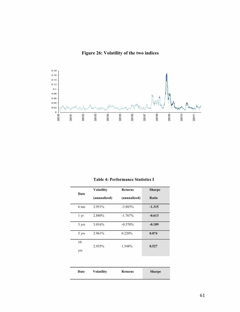
Figure 26: Volatility of the two indices

Table 4: Performance Statistics I

Date Volatility

(annualized)

Returns

(annualized)

Sharpe

Ratio

6 mo 2.951% -3.883% -1.315

1 yr 2.880% -1.767% -0.613

3 yrs 3.016% -0.570% -0.189

5 yrs 2.961% 0.220% 0.074

10

yrs 2.935% 1.548% 0.527

Date Volatility Returns Sharpe

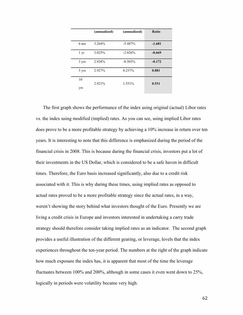
62

(annualized) (annualized) Ratio

6 mo 3.264% -5.487% -1.681

1 yr 3.025% -2.026% -0.669

3 yrs 2.928% -0.503% -0.172

5 yrs 2.927% 0.237% 0.081

10

yrs 2.921% 1.551% 0.531

The first graph shows the performance of the index using original (actual) Libor rates

vs. the index using modified (implied) rates. As you can see, using implied Libor rates

does prove to be a more profitable strategy by achieving a 10% increase in return over ten

years. It is interesting to note that this difference is emphasized during the period of the

financial crisis in 2008. This is because during the financial crisis, investors put a lot of

their investments in the US Dollar, which is considered to be a safe haven in difficult

times. Therefore, the Euro basis increased significantly, also due to a credit risk

associated with it. This is why during these times, using implied rates as opposed to

actual rates proved to be a more profitable strategy since the actual rates, in a way,

weren’t showing the story behind what investors thought of the Euro. Presently we are

living a credit crisis in Europe and investors interested in undertaking a carry trade

strategy should therefore consider taking implied rates as an indicator. The second graph

provides a useful illustration of the different gearing, or leverage, levels that the index

experiences throughout the ten-year period. The numbers at the right of the graph indicate

how much exposure the index has, it is apparent that most of the time the leverage

fluctuates between 100% and 200%, although in some cases it even went down to 25%,

logically in periods were volatility became very high.

63

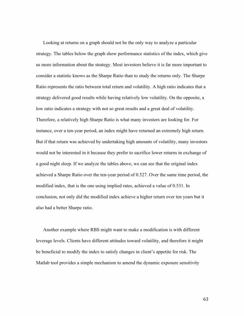
Looking at returns on a graph should not be the only way to analyze a particular

strategy. The tables below the graph show performance statistics of the index, which give

us more information about the strategy. Most investors believe it is far more important to

consider a statistic knows as the Sharpe Ratio than to study the returns only. The Sharpe

Ratio represents the ratio between total return and volatility. A high ratio indicates that a

strategy delivered good results while having relatively low volatility. On the opposite, a

low ratio indicates a strategy with not so great results and a great deal of volatility.

Therefore, a relatively high Sharpe Ratio is what many investors are looking for. For

instance, over a ten-year period, an index might have returned an extremely high return.

But if that return was achieved by undertaking high amounts of volatility, many investors

would not be interested in it because they prefer to sacrifice lower returns in exchange of

a good night sleep. If we analyze the tables above, we can see that the original index

achieved a Sharpe Ratio over the ten-year period of 0.527. Over the same time period, the

modified index, that is the one using implied rates, achieved a value of 0.531. In

conclusion, not only did the modified index achieve a higher return over ten years but it

also had a better Sharpe ratio.

Another example where RBS might want to make a modification is with different

leverage levels. Clients have different attitudes toward volatility, and therefore it might

be beneficial to modify the index to satisfy changes in client’s appetite for risk. The

Matlab tool provides a simple mechanism to amend the dynamic exposure sensitivity

64

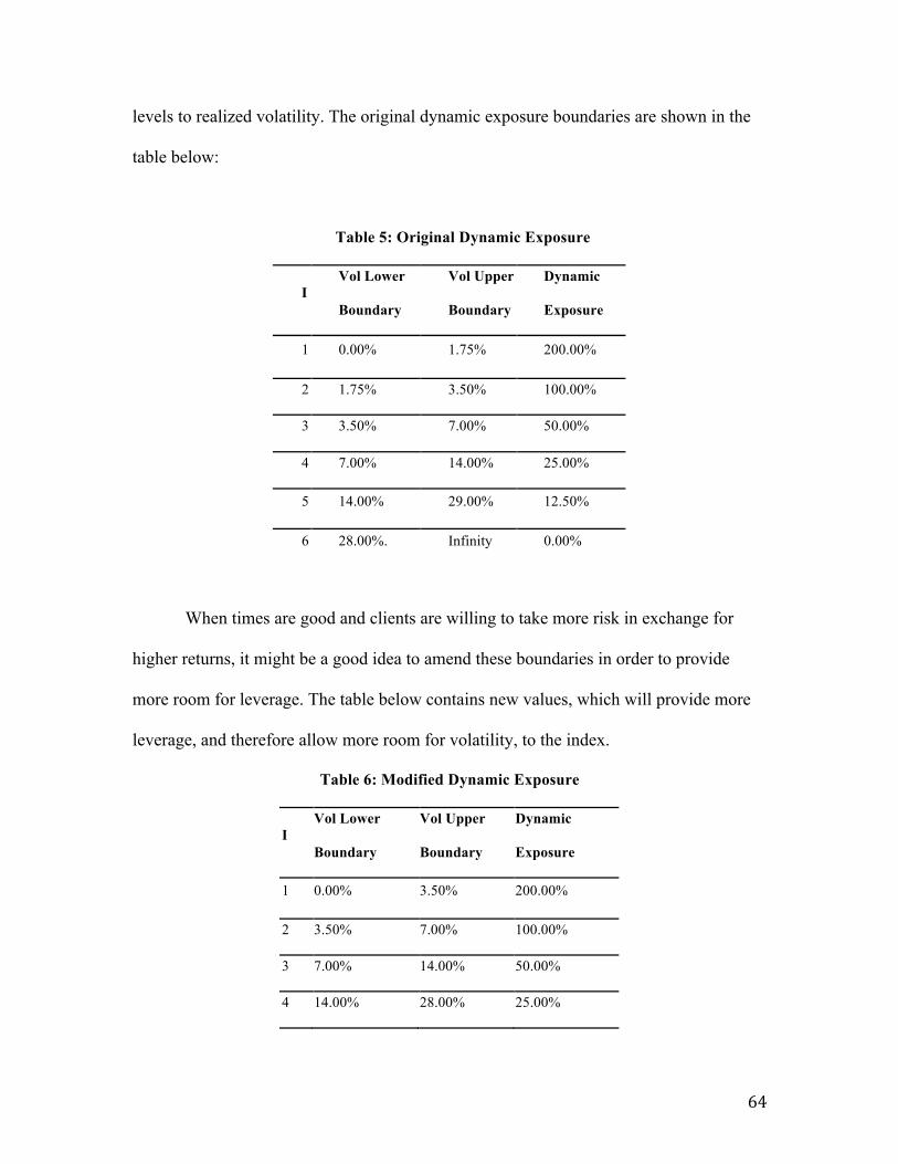
levels to realized volatility. The original dynamic exposure boundaries are shown in the

table below:

Table 5: Original Dynamic Exposure

I Vol Lower

Boundary

Vol Upper

Boundary

Dynamic

Exposure

1 0.00% 1.75% 200.00%

2 1.75% 3.50% 100.00%

3 3.50% 7.00% 50.00%

4 7.00% 14.00% 25.00%

5 14.00% 29.00% 12.50%

6 28.00%. Infinity 0.00%

When times are good and clients are willing to take more risk in exchange for

higher returns, it might be a good idea to amend these boundaries in order to provide

more room for leverage. The table below contains new values, which will provide more

leverage, and therefore allow more room for volatility, to the index.

Table 6: Modified Dynamic Exposure

I Vol Lower

Boundary

Vol Upper

Boundary

Dynamic

Exposure

1 0.00% 3.50% 200.00%

2 3.50% 7.00% 100.00%

3 7.00% 14.00% 50.00%

4 14.00% 28.00% 25.00%

65

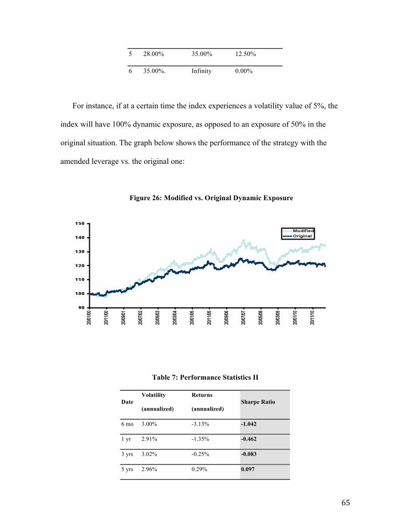
5 28.00% 35.00% 12.50%

6 35.00%. Infinity 0.00%

For instance, if at a certain time the index experiences a volatility value of 5%, the

index will have 100% dynamic exposure, as opposed to an exposure of 50% in the

original situation. The graph below shows the performance of the strategy with the

amended leverage vs. the original one:

Figure 26: Modified vs. Original Dynamic Exposure

Table 7: Performance Statistics II

Date Volatility

(annualized)

Returns

(annualized) Sharpe Ratio

6 mo 3.00% -3.13% -1.042

1 yr 2.91% -1.35% -0.462

3 yrs 3.02% -0.25% -0.083

5 yrs 2.96% 0.29% 0.097

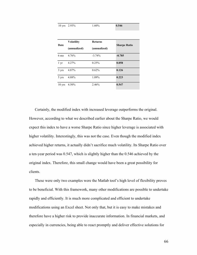
66

10 yrs 2.93% 1.60% 0.546

Date Volatility

(annualized)

Returns

(annualized) Sharpe Ratio

6 mo 4.76% -3.74% -0.785

1 yr 4.27% 0.25% 0.058

3 yrs 4.87% 0.62% 0.126

5 yrs 4.88% 1.09% 0.223

10 yrs 4.50% 2.46% 0.547

Certainly, the modified index with increased leverage outperforms the original.

However, according to what we described earlier about the Sharpe Ratio, we would

expect this index to have a worse Sharpe Ratio since higher leverage is associated with

higher volatility. Interestingly, this was not the case. Even though the modified index

achieved higher returns, it actually didn’t sacrifice much volatility. Its Sharpe Ratio over

a ten-year period was 0.547, which is slightly higher than the 0.546 achieved by the

original index. Therefore, this small change would have been a great possibility for

clients.

These were only two examples were the Matlab tool’s high level of flexibility proves

to be beneficial. With this framework, many other modifications are possible to undertake

rapidly and efficiently. It is much more complicated and efficient to undertake

modifications using an Excel sheet. Not only that, but it is easy to make mistakes and

therefore have a higher risk to provide inaccurate information. In financial markets, and

especially in currencies, being able to react promptly and deliver effective solutions for

67

clients is essential and having a mechanism that allows amendments to be made in a short

period of time is valuable.

68

Impact of Project and Conclusions

Our MQP project gave us the opportunity to work in a world-class investment bank

and to be part of a great team involved with Structuring in foreign exchange. We were

given a challenge, which was to help the Structuring team build a new tool that will

enable them to compete with the big players in the FX Index business and to offer clients

the best high-touch service to their solutions. By introducing Matlab to the team, we were

able to create a significant positive impact to RBS. The main impacts of our project were:

• 50% reduced index development time. We have roughly calculated that building a

new index from scratch using the introduced Matlab tool will take at least half the

time than if the index were created using Excel. In a high paced environment such

as the financial industry where many things happen in a matter of minutes, this

reduced time will prove to be beneficial to the team.

• 10 % total timesaving per week to back test indices. In addition to the timesaving

regarding index development time, our Matlab tool will also decrease by more

than 10% the time required to back test indices. As an example of this, Richard

Groenewegen, who is in charge of FX index development in RBS, discovered that

by using the tool he did a lot of back testing of the indices in a significantly

shorter time than it took before. Since he has to compare his results of his indices

to third parties such as Markit, these time savings help not only the RBS team, but

69

it also enhances interaction with Markit and all other parties involved with the

creation of the indices.

• Higher flexibility to make variations to index. The Matlab tool is highly versatile

since the code enables the user to modify parameters and get the new results

quickly. This helps RBS deliver the best solutions to their clients, tailored their

specific needs.

• Reduced risk for human error. The macro view that Matlab provides reduces

room for mistakes since it is much easier to see the big picture and to not get lost

in the “index maze”. Previously, the excel sheets had to contain many manual

instructions warning the user not to modify certain columns and this mechanism

created a lot of risks to make errors.

• Cleaner process and higher power for complex indices. Lastly, but certainly not

least, the new framework looks cleaner while at the same time being more

powerful, opening opportunities to create more ambitious indexes that will aid

clients with their investments in highly volatile times like these. The cleanliness

also helps when in the future new employees become part of the structuring team

and a simple framework will lower the learning curve and allow them to add

value to the team promptly.

70

All of these things will help RBS to gain market share in the FX index business.

However, more importantly, it will aid the Structuring team deliver better, more powerful

indices to clients while taking less time to do so. Even though the time reductions are

represented in hours, these will make an economic impact since the extra time will enable

the team do more structures and deals with clients.

71

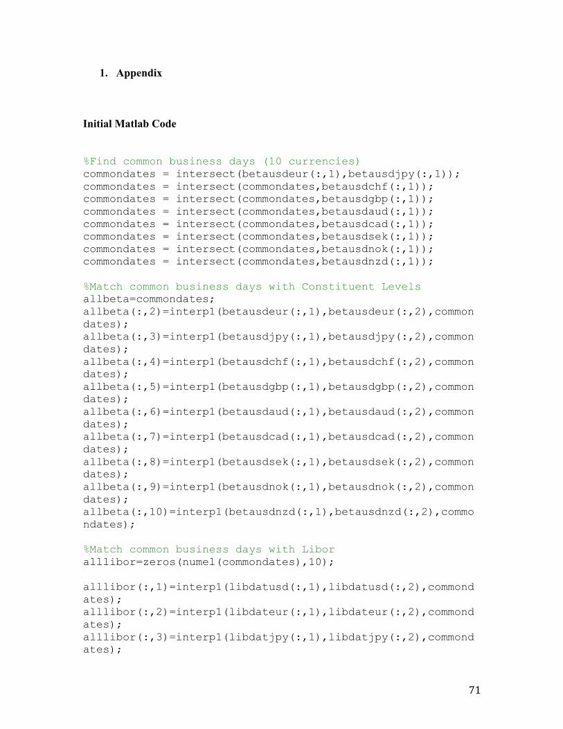
1. Appendix

Initial Matlab Code

%Find common business days (10 currencies) commondates = intersect(betausdeur(:,1),betausdjpy(:,1)); commondates = intersect(commondates,betausdchf(:,1)); commondates = intersect(commondates,betausdgbp(:,1)); commondates = intersect(commondates,betausdaud(:,1)); commondates = intersect(commondates,betausdcad(:,1)); commondates = intersect(commondates,betausdsek(:,1)); commondates = intersect(commondates,betausdnok(:,1)); commondates = intersect(commondates,betausdnzd(:,1)); %Match common business days with Constituent Levels allbeta=commondates; allbeta(:,2)=interp1(betausdeur(:,1),betausdeur(:,2),commondates); allbeta(:,3)=interp1(betausdjpy(:,1),betausdjpy(:,2),commondates); allbeta(:,4)=interp1(betausdchf(:,1),betausdchf(:,2),commondates); allbeta(:,5)=interp1(betausdgbp(:,1),betausdgbp(:,2),commondates); allbeta(:,6)=interp1(betausdaud(:,1),betausdaud(:,2),commondates); allbeta(:,7)=interp1(betausdcad(:,1),betausdcad(:,2),commondates); allbeta(:,8)=interp1(betausdsek(:,1),betausdsek(:,2),commondates); allbeta(:,9)=interp1(betausdnok(:,1),betausdnok(:,2),commondates); allbeta(:,10)=interp1(betausdnzd(:,1),betausdnzd(:,2),commondates); %Match common business days with Libor alllibor=zeros(numel(commondates),10); alllibor(:,1)=interp1(libdatusd(:,1),libdatusd(:,2),commondates); alllibor(:,2)=interp1(libdateur(:,1),libdateur(:,2),commondates); alllibor(:,3)=interp1(libdatjpy(:,1),libdatjpy(:,2),commondates);

72

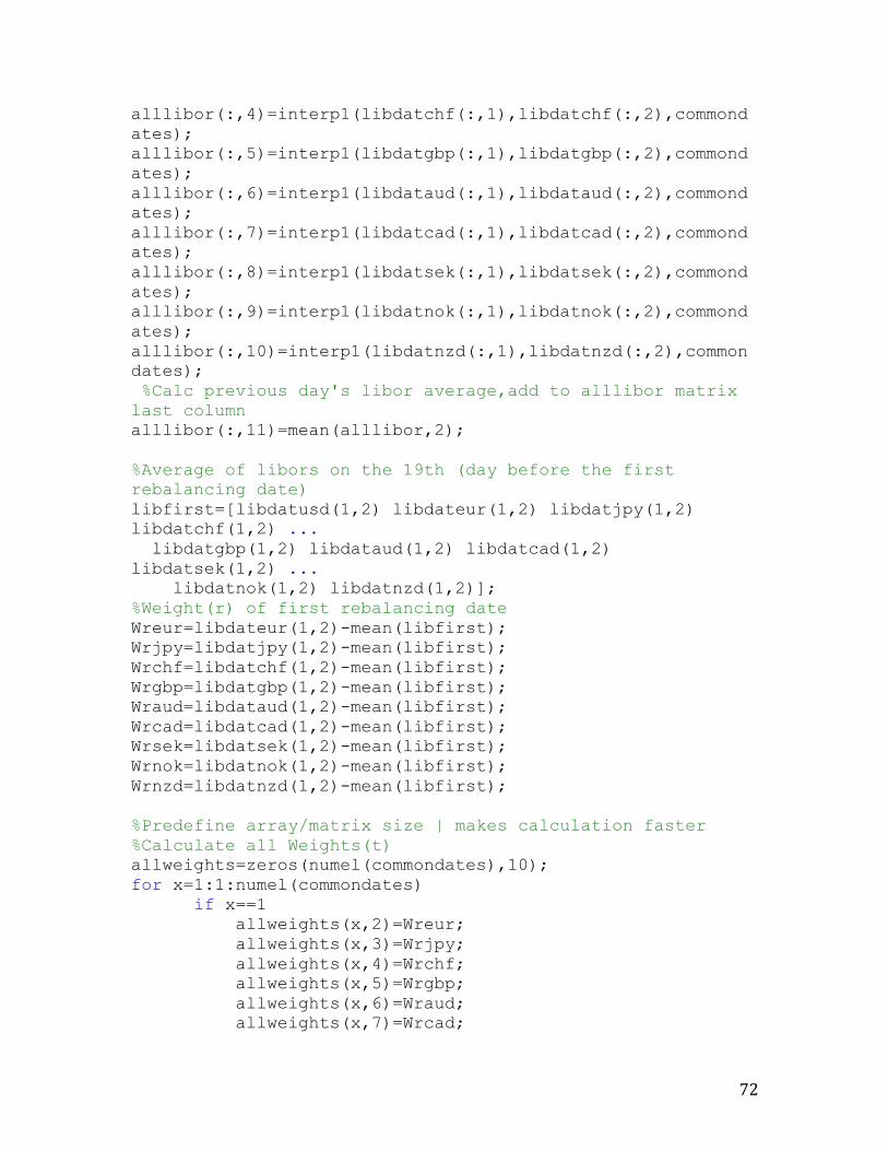
alllibor(:,4)=interp1(libdatchf(:,1),libdatchf(:,2),commondates); alllibor(:,5)=interp1(libdatgbp(:,1),libdatgbp(:,2),commondates); alllibor(:,6)=interp1(libdataud(:,1),libdataud(:,2),commondates); alllibor(:,7)=interp1(libdatcad(:,1),libdatcad(:,2),commondates); alllibor(:,8)=interp1(libdatsek(:,1),libdatsek(:,2),commondates); alllibor(:,9)=interp1(libdatnok(:,1),libdatnok(:,2),commondates); alllibor(:,10)=interp1(libdatnzd(:,1),libdatnzd(:,2),commondates); %Calc previous day's libor average,add to alllibor matrix last column alllibor(:,11)=mean(alllibor,2); %Average of libors on the 19th (day before the first rebalancing date) libfirst=[libdatusd(1,2) libdateur(1,2) libdatjpy(1,2) libdatchf(1,2) ... libdatgbp(1,2) libdataud(1,2) libdatcad(1,2) libdatsek(1,2) ... libdatnok(1,2) libdatnzd(1,2)]; %Weight(r) of first rebalancing date Wreur=libdateur(1,2)-mean(libfirst); Wrjpy=libdatjpy(1,2)-mean(libfirst); Wrchf=libdatchf(1,2)-mean(libfirst); Wrgbp=libdatgbp(1,2)-mean(libfirst); Wraud=libdataud(1,2)-mean(libfirst); Wrcad=libdatcad(1,2)-mean(libfirst); Wrsek=libdatsek(1,2)-mean(libfirst); Wrnok=libdatnok(1,2)-mean(libfirst); Wrnzd=libdatnzd(1,2)-mean(libfirst); %Predefine array/matrix size | makes calculation faster %Calculate all Weights(t) allweights=zeros(numel(commondates),10); for x=1:1:numel(commondates) if x==1 allweights(x,2)=Wreur; allweights(x,3)=Wrjpy; allweights(x,4)=Wrchf; allweights(x,5)=Wrgbp; allweights(x,6)=Wraud; allweights(x,7)=Wrcad;

73

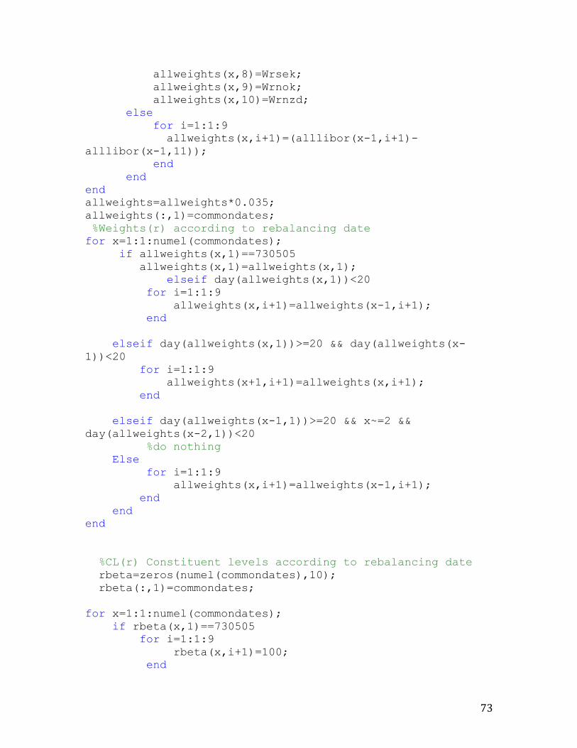
allweights(x,8)=Wrsek; allweights(x,9)=Wrnok; allweights(x,10)=Wrnzd; else for i=1:1:9 allweights(x,i+1)=(alllibor(x-1,i+1)-alllibor(x-1,11)); end end end allweights=allweights*0.035; allweights(:,1)=commondates; %Weights(r) according to rebalancing date for x=1:1:numel(commondates); if allweights(x,1)==730505 allweights(x,1)=allweights(x,1); elseif day(allweights(x,1))<20 for i=1:1:9 allweights(x,i+1)=allweights(x-1,i+1); end elseif day(allweights(x,1))>=20 && day(allweights(x-1))<20 for i=1:1:9 allweights(x+1,i+1)=allweights(x,i+1); end elseif day(allweights(x-1,1))>=20 && x~=2 && day(allweights(x-2,1))<20 %do nothing Else for i=1:1:9 allweights(x,i+1)=allweights(x-1,i+1); end end end %CL(r) Constituent levels according to rebalancing date rbeta=zeros(numel(commondates),10); rbeta(:,1)=commondates; for x=1:1:numel(commondates); if rbeta(x,1)==730505 for i=1:1:9 rbeta(x,i+1)=100; end

74

elseif day(allbeta(x,1))<20 for i=1:1:9 rbeta(x,i+1)=rbeta(x-1,i+1); end elseif day(rbeta(x-1,1))>=20 && x~=2 && day(rbeta(x-2,1))<20 for i=1:1:9 rbeta(x,i+1)=allbeta(x-1,i+1); end else for i=1:1:9 rbeta(x,i+1)=rbeta(x-1,i+1); end end end %Create matrix with underlying returns ureturns=zeros(numel(commondates),11); ureturns(:,1)=commondates; for x=1:1:numel(commondates) if day(ureturns(x,1))>=20 && x~=1 && day(ureturns(x-1,1))<20 for i=1:1:9 ureturns(x,i+1)=allweights(x-1,i+1).*((allbeta(x,i+1)-rbeta(x,i+1))/100); end ureturns(x,11)=ureturns(x,2)+ureturns(x,3)+ureturns(x,4)+ureturns(x,5)+ureturns(x,6)+... ureturns(x,7)+ureturns(x,8)+ureturns(x,9)+ureturns(x,10); else for i=1:1:9 ureturns(x,i+1)=allweights(x,i+1).*((allbeta(x,i+1)-rbeta(x,i+1))/100); end ureturns(x,11)=ureturns(x,2)+ureturns(x,3)+ureturns(x,4)+ureturns(x,5)+ureturns(x,6)+... ureturns(x,7)+ureturns(x,8)+ureturns(x,9)+ureturns(x,10); end end

75

%Matrix with relative Spread spreadi=[0.00035 0.0003 0.0008 0.0004 0.0005 0.00105 0.0006 0.0018 0.00065]; %Calculate trading cost tradingcost=zeros(numel(commondates),11); tradingcost(:,1)=commondates; for x=1:1:numel(commondates) if tradingcost(x,1)==730505 for i=1:1:10 tradingcost(x,i+1)=0; end elseif day(tradingcost(x,1))>=20 && day(tradingcost(x-1,1))<20 total=0; for i=1:1:9 total=abs(allweights(x,i+1))*spreadi(i)+total; tradingcost(x,i+1)=abs(allweights(x,i+1))*spreadi(i); end tradingcost(x,11)=total; end end %Core Index Calculation coreindex=zeros(numel(commondates),3); coreindex(:,1)=commondates; for x=1:1:numel(commondates) if coreindex(x,1)==730505 coreindex(x,2)=100; coreindex(x,3)=100; elseif day(coreindex(x,1))>=20 && day(coreindex(x-1,1))<20 coreindex(x,2)=coreindex(x-1,2); coreindex(x,3)=coreindex(x,2).*(1+ureturns(x,11)-tradingcost(x,11)); elseif day(coreindex(x-1,1))>=20 && x~=2 && day(coreindex(x-2,1))<20 coreindex(x,2)=coreindex(x-1,3); coreindex(x,3)=coreindex(x,2).*(1+ureturns(x,11)-tradingcost(x,11)); else coreindex(x,2)=coreindex(x-1,2); coreindex(x,3)=coreindex(x,2).*(1+ureturns(x,11)-tradingcost(x,11)); end

76

end %Calculate return hihihihihi returnvc=zeros(numel(commondates),2); for x=1:1:numel(commondates) if x==1 returnvc(x,2)=0; else returnvc(x,2)=coreindex(x,3)/coreindex(x-1,3)-1; end end %Matrix for portfolio returns (ln and sums) lnportreturn=zeros(numel(commondates),22); %Calculate Realized Volatility for x=1:1:numel(commondates) if x>=1 && x<23 for i=2:1:21 lnportreturn(x,i)=0; end else if day(lnportreturn(x,1))>=20 && day(lnportreturn(x-1,1))<20 w1=allweights(x-1,2);w2=allweights(x-1,3);w3=allweights(x-1,4); w4=allweights(x-1,5);w5=allweights(x-1,6);w6=allweights(x-1,7); w7=allweights(x-1,8);w8=allweights(x-1,9);w9=allweights(x-1,10); else w1=allweights(x,2);w2=allweights(x,3);w3=allweights(x,4); w4=allweights(x,5);w5=allweights(x,6);w6=allweights(x,7); w7=allweights(x,8);w8=allweights(x,9);w9=allweights(x,10); end for i=2:1:21 lnportreturn(x,i)=log(1+w1*(allbeta(x+2-i,2)-allbeta(x+1-i,2))/100+... w2*(allbeta(x-i+2,3)-allbeta(x+1-i,3))/100+...

77

w3*(allbeta(x-i+2,4)-allbeta(x+1-i,4))/100+... w4*(allbeta(x-i+2,5)-allbeta(x+1-i,5))/100+... w5*(allbeta(x-i+2,6)-allbeta(x+1-i,6))/100+... w6*(allbeta(x-i+2,7)-allbeta(x+1-i,7))/100+... w7*(allbeta(x-i+2,8)-allbeta(x+1-i,8))/100+... w8*(allbeta(x-i+2,9)-allbeta(x+1-i,9))/100+... w9*(allbeta(x-i+2,10)-allbeta(x+1-i,10))/100); end end lnportreturn(x,22)=sqrt(252)*std(lnportreturn(x,2:21),0,2); end lnportreturn(:,1)=commondates; %Define Index Matrix which includes Realized Vol, Dynammic %Exposure,Trading Cost, Index Level (VC) vcindex=zeros(numel(commondates),5); vcindex(:,1)=commondates; vcindex(:,2)=lnportreturn(:,22); %Calculate Dynamic Exposure for x=23:1:numel(commondates) if vcindex(x,2)<0.035 vcindex(x,3)=2; elseif vcindex(x,2)<0.07 vcindex(x,3)=1; elseif vcindex(x,2)<0.14 vcindex(x,3)=0.5; elseif vcindex(x,2)<0.28 vcindex(x,3)=0.25; else vcindex(x,3)=0.125; end end %Calculate trading cost tc=0; for x=25:1:numel(commondates)

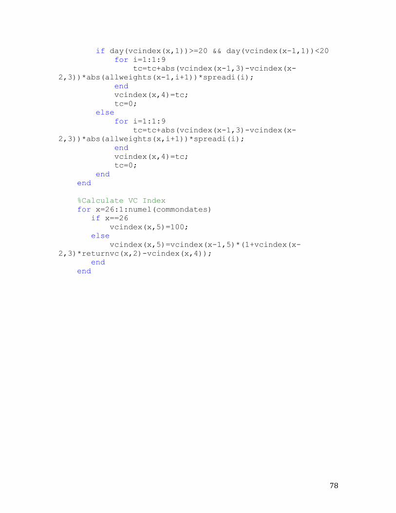
78

if day(vcindex(x,1))>=20 && day(vcindex(x-1,1))<20 for i=1:1:9 tc=tc+abs(vcindex(x-1,3)-vcindex(x-2,3))*abs(allweights(x-1,i+1))*spreadi(i); end vcindex(x,4)=tc; tc=0; else for i=1:1:9 tc=tc+abs(vcindex(x-1,3)-vcindex(x-2,3))*abs(allweights(x,i+1))*spreadi(i); end vcindex(x,4)=tc; tc=0; end end %Calculate VC Index for x=26:1:numel(commondates) if x==26 vcindex(x,5)=100; else vcindex(x,5)=vcindex(x-1,5)*(1+vcindex(x-2,3)*returnvc(x,2)-vcindex(x,4)); end end

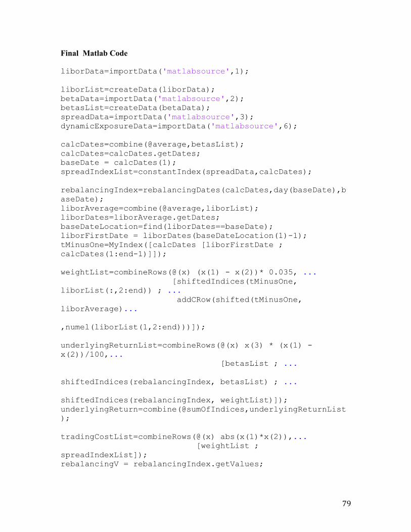
79

Final Matlab Code liborData=importData('matlabsource',1);

liborList=createData(liborData); betaData=importData('matlabsource',2); betasList=createData(betaData); spreadData=importData('matlabsource',3); dynamicExposureData=importData('matlabsource',6); calcDates=combine(@average,betasList); calcDates=calcDates.getDates; baseDate = calcDates(1); spreadIndexList=constantIndex(spreadData,calcDates); rebalancingIndex=rebalancingDates(calcDates,day(baseDate),baseDate); liborAverage=combine(@average,liborList); liborDates=liborAverage.getDates; baseDateLocation=find(liborDates==baseDate); liborFirstDate = liborDates(baseDateLocation(1)-1); tMinusOne=MyIndex([calcDates [liborFirstDate ; calcDates(1:end-1)]]); weightList=combineRows(@(x) (x(1) - x(2))* 0.035, ... [shiftedIndices(tMinusOne, liborList(:,2:end)) ; ... addCRow(shifted(tMinusOne, liborAverage)... ,numel(liborList(1,2:end)))]); underlyingReturnList=combineRows(@(x) x(3) * (x(1) - x(2))/100,... [betasList ; ... shiftedIndices(rebalancingIndex, betasList) ; ... shiftedIndices(rebalancingIndex, weightList)]); underlyingReturn=combine(@sumOfIndices,underlyingReturnList); tradingCostList=combineRows(@(x) abs(x(1)*x(2)),... [weightList ; spreadIndexList]); rebalancingV = rebalancingIndex.getValues;

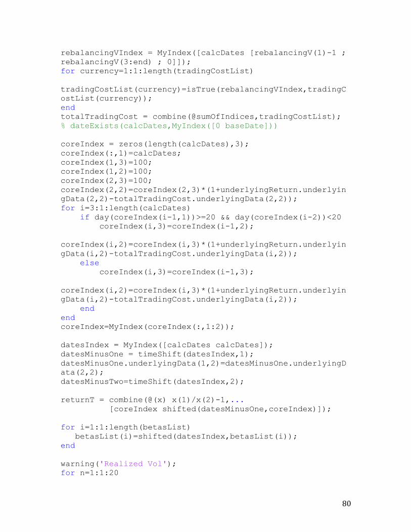
80

rebalancingVIndex = MyIndex([calcDates [rebalancingV(1)-1 ; rebalancingV(3:end) ; 0]]); for currency=1:1:length(tradingCostList) tradingCostList(currency)=isTrue(rebalancingVIndex,tradingCostList(currency)); end totalTradingCost = combine(@sumOfIndices,tradingCostList); % dateExists(calcDates,MyIndex([0 baseDate])) coreIndex = zeros(length(calcDates),3); coreIndex(:,1)=calcDates; coreIndex(1,3)=100; coreIndex(1,2)=100; coreIndex(2,3)=100; coreIndex(2,2)=coreIndex(2,3)*(1+underlyingReturn.underlyingData(2,2)-totalTradingCost.underlyingData(2,2)); for i=3:1:length(calcDates) if day(coreIndex(i-1,1))>=20 && day(coreIndex(i-2))<20 coreIndex(i,3)=coreIndex(i-1,2); coreIndex(i,2)=coreIndex(i,3)*(1+underlyingReturn.underlyingData(i,2)-totalTradingCost.underlyingData(i,2)); else coreIndex(i,3)=coreIndex(i-1,3); coreIndex(i,2)=coreIndex(i,3)*(1+underlyingReturn.underlyingData(i,2)-totalTradingCost.underlyingData(i,2)); end end coreIndex=MyIndex(coreIndex(:,1:2)); datesIndex = MyIndex([calcDates calcDates]); datesMinusOne = timeShift(datesIndex,1); datesMinusOne.underlyingData(1,2)=datesMinusOne.underlyingData(2,2); datesMinusTwo=timeShift(datesIndex,2); returnT = combine(@(x) x(1)/x(2)-1,... [coreIndex shifted(datesMinusOne,coreIndex)]); for i=1:1:length(betasList) betasList(i)=shifted(datesIndex,betasList(i)); end warning('Realized Vol'); for n=1:1:20

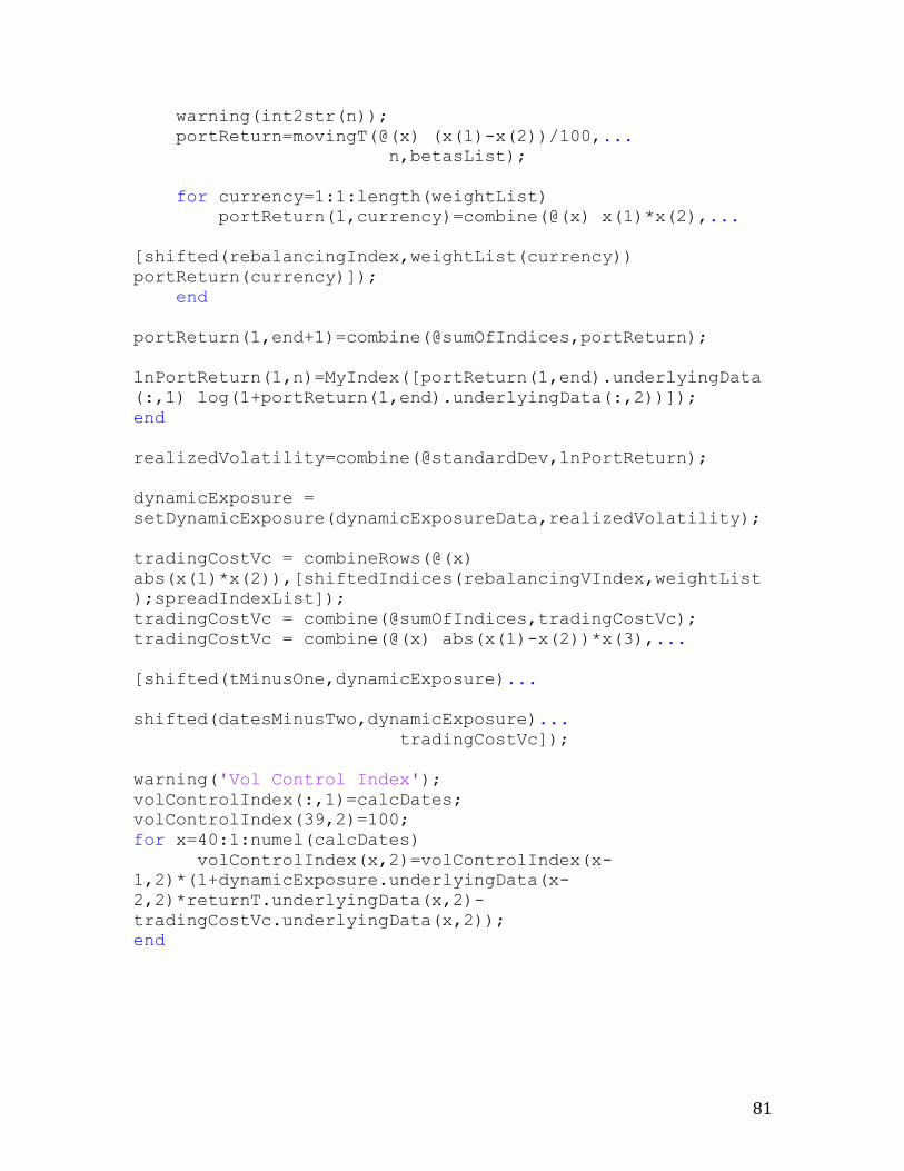
81

warning(int2str(n)); portReturn=movingT(@(x) (x(1)-x(2))/100,... n,betasList); for currency=1:1:length(weightList) portReturn(1,currency)=combine(@(x) x(1)*x(2),... [shifted(rebalancingIndex,weightList(currency)) portReturn(currency)]); end portReturn(1,end+1)=combine(@sumOfIndices,portReturn); lnPortReturn(1,n)=MyIndex([portReturn(1,end).underlyingData(:,1) log(1+portReturn(1,end).underlyingData(:,2))]); end realizedVolatility=combine(@standardDev,lnPortReturn); dynamicExposure = setDynamicExposure(dynamicExposureData,realizedVolatility); tradingCostVc = combineRows(@(x) abs(x(1)*x(2)),[shiftedIndices(rebalancingVIndex,weightList);spreadIndexList]); tradingCostVc = combine(@sumOfIndices,tradingCostVc); tradingCostVc = combine(@(x) abs(x(1)-x(2))*x(3),... [shifted(tMinusOne,dynamicExposure)... shifted(datesMinusTwo,dynamicExposure)... tradingCostVc]); warning('Vol Control Index'); volControlIndex(:,1)=calcDates; volControlIndex(39,2)=100; for x=40:1:numel(calcDates) volControlIndex(x,2)=volControlIndex(x-1,2)*(1+dynamicExposure.underlyingData(x-2,2)*returnT.underlyingData(x,2)-tradingCostVc.underlyingData(x,2)); end

82

2. References

1) Interviews with David Popplewell, Richard Groenewegen and Ben Nicklin

2) Investopedia (n.d). Retrieved from October 25th 2011 from

http://www.investopedia.com/

3) RBS- Global Portal (n.d). Retrieved from http://www.rbs.com

4) "Top Banks in the World 2011." Banks of the World. RelBanks, 31 Dec. 2011. Web. 29 Feb. 2012. <http://www.relbanks.com/worlds-top-banks/assets-2011>.