BACHELOR THESIS

Advanced Technology

CONTACT MECHANICS IN MSC ADAMS

A technical evaluation of the contact models in

multibody dynamics software MSC Adams

Author

Jochem Giesbers

Faculty of Engineering Technology

Applied Mechanics

Examination Committee

Chairperson: Prof. Dr. Ir. A. de Boer

Supervisor: Dr. Ir. M.H.M. Ellenbroek

External examiner: Dr. H.K. Hemmes

Member: Dr. Ir. P.J.M. van der Hoogt

July 11th, 2012

Page | 2

Abstract: The goal of this study is to gain insight in the modelling of (physical) contact in Adams, a product by MSC

Software. Adams is the most widely used multibody dynamics and motion analysis software in the world.

The aim is to establish an understanding of contact in Adams and the relation to the laws of physics. First,

the algorithms and formulas used by Adams are analysed. Second, a variety of models is simulated and the

effects of the corresponding variables are analysed. After this study the acquired knowledge can be used to

model more complex systems in Adams.

Page | 3

Table of Contents

Abstract: ........................................................................................................................................................ 2

Table of Contents ........................................................................................................................................... 3

1. Introduction: ............................................................................................................................................ 5

2. Theory: ..................................................................................................................................................... 6

2.1 Hertzian contact theory ...................................................................................................................... 6

2.2 Hertzian contact theory in relation to the IMPACT function ................................................................ 7

2.3 Geometry engines .............................................................................................................................. 8

2.4 Normal force ...................................................................................................................................... 9

2.5 Friction ............................................................................................................................................. 10

2.6 Contact feature: IMPACT function model ......................................................................................... 11

2.7 Contact feature: POISSON restitution model .................................................................................... 13

2.8 Contact feature: Coulomb friction .................................................................................................... 14

3. Cases:..................................................................................................................................................... 15

3.1 Introduction ..................................................................................................................................... 15

3.2 Bouncing ball (2D) ............................................................................................................................ 16

3.2.1 IMPACT function: ....................................................................................................................... 17

3.2.2 POISSON restitution: .................................................................................................................. 19

3.2.3 Discussion:................................................................................................................................. 20

3.3 Rolling ball (2D) ................................................................................................................................ 21

3.3.1 Suitable normal force configuration ........................................................................................... 22

3.3.2 Coulomb friction model ............................................................................................................. 23

3.3.3 Discussion:................................................................................................................................. 25

4. Recommended values:............................................................................................................................ 27

4.1 Introduction ..................................................................................................................................... 27

4.2 IMPACT function model .................................................................................................................... 28

4.2.1 Stiffness :................................................................................................................................. 28

4.2.2 Force exponent : ...................................................................................................................... 28

4.2.3 Maximum damping : ........................................................................................................ 28

4.2.4 Penetration depth : ................................................................................................................. 28

4.3 POISSON restitution model ............................................................................................................... 29

4.3.1 Coefficient of Restitution : .................................................................................................. 29

4.3.2 Penalty : .................................................................................................................................. 29

Page | 4

4.4 Coulomb friction model .................................................................................................................... 30

4.4.1 Coefficient of friction and : ............................................................................................... 30

4.4.2 Transition velocity and : ................................................................................................... 30

5. Conclusion: ............................................................................................................................................. 31

6. Recommendations:................................................................................................................................. 32

Appendix A (Bouncing Ball Graphs): ............................................................................................................. 33

Appendix B (Rolling Ball Graphs): ................................................................................................................. 37

Appendix C (Material Contact Properties): ................................................................................................... 42

Page | 5

1. Introduction:

This report has been written to finalize the bachelor Advanced Technology assignment that has been done in

the Applied Mechanics research chair of the University of Twente.

Contact between objects is an important aspect in multibody dynamics. It is a discontinuous, non-linear

phenomenon and therefore requires iterative calculations. Adams, a MSC Software product in multibody

dynamics, performs these calculations and can provide accurate results. The accuracy depends on user-

defined values, so it is of importance that the user has knowledge of the program, the algorithms and the

variables.

This report shall first deal with the relevant theory and background information of contact forces and three

built-in contact methods of Adams; the IMPACT function model, the POISSON restitution model and the

Coulomb friction model. Subsequently these three contact methods are evaluated and discussed by the use

of two self-constructed Adams models. All parameters in these three contact methods are varied to research

their effect on the contact behaviour. Subsequently the recommended values for all the parameters are

determined. Finally, conclusions are drawn and recommendations for further research are made.

A word of thanks extends to my supervisor Dr. Ir. M.H.M. Ellenbroek for providing insight, help and

understanding throughout the process of this bachelor assignment.

Page | 6

2. Theory:

2.1 Hertzian contact theory

In contact mechanics there are multiple models for predicting contact forces and geometrical deformations.

In 1882, Heinrich Hertz published a theory concerning circular contact areas and elastic deformations in the

case of contact between two spheres1. In this theory the Van der Waals interactions and other adhesive

interactions are neglected. It was not until 1970 that Johnson, Kendall and Roberts published a theory that is

largely the same, but includes adhesion in the contact area2.

Hertzian theory is based on a set of assumptions, which are as follows:

Adhesion is neglected. Contacting bodies can be separated without adhesion forces.

Surfaces are continuous and non-conforming, i.e. the initial contact is a point or a line.

Pressures within the materials are small enough to cause only elastic deformations.

The area of contact is much smaller than the characteristic radius of the body.

The surfaces are perfectly smooth, i.e. only a normal force acts between the parts in contact.

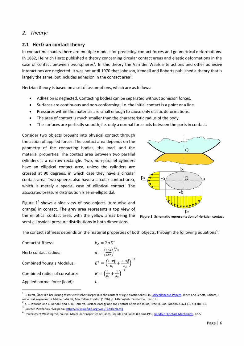
Consider two objects brought into physical contact through

the action of applied forces. The contact area depends on the

geometry of the contacting bodies, the load, and the

material properties. The contact area between two parallel

cylinders is a narrow rectangle. Two, non-parallel cylinders

have an elliptical contact area, unless the cylinders are

crossed at 90 degrees, in which case they have a circular

contact area. Two spheres also have a circular contact area,

which is merely a special case of elliptical contact. The

associated pressure distribution is semi-ellipsoidal.

Figure 13 shows a side view of two objects (turquoise and

orange) in contact. The grey area represents a top view of

the elliptical contact area, with the yellow areas being the

semi-ellipsoidal pressure distributions in both dimensions.

The contact stiffness depends on the material properties of both objects, through the following equations4:

Contact stiffness:

Hertz contact radius:

Combined Young’s Modulus:

Combined radius of curvature:

Applied normal force (load):

1 H. Hertz, Über die berührung fester elastischer Körper (On the contact of rigid elastic solids). In: Miscellaneous Papers. Jones and Schott, Editors, J.

reine und angewandte Mathematik 92, Macmillan, London (1896), p. 146 English translation: Hertz, H. 2 K. L. Johnson and K. Kendall and A. D. Roberts, Surface energy and the contact of elastic solids, Proc. R. Soc. London A 324 (1971) 301-313

3 Contact Mechanics, Wikipedia; http://en.wikipedia.org/wiki/File:Hertz.svg

4 University of Washington, course: Molecular Properties of Gases, Liquids and Solids (ChemE498), handout ‘Contact Mechanics’, p2-5

Figure 1: Schematic representation of Hertzian contact

Page | 7

2.2 Hertzian contact theory in relation to the IMPACT function

This chapter is based on a misconception and therefore contains incorrect information.

One of the methods that Adams uses is extrapolated from Hertzian contact theory: the Adams IMPACT

function. A detailed description of the IMPACT function will follow in Chapter 2.6. A brief description of the

relation between the IMPACT function and the Hertzian contact theory as described in Chapter 2.1 will

follow now.

In Chapter 2.1 a set of formulas for the contact stiffness was proposed, from which the normal force follows:

In the formula above a linear spring force can be recognized (if would be constant). Its value depends on a

stiffness parameter and the penetration depth . The stiffness depends on both materials’ Young’s

Moduli and Poisson’s Ratios, both objects’ radii and the force with which the objects are pressed together.

The IMPACT function uses a stiffness parameter that is related to the Hertzian contact stiffness. However,

the load appears to vary with the penetration depth. A greater penetration depth leads to a greater

restoring normal force ( ). Therefore the contact stiffness is not constant, making the force non-linear. It is

believed that because of this non-linearity, the IMPACT function does not only use a static stiffness

parameter ( ), but also an additional force exponent ( ):

In this formula the stiffness is constant, so the non-linearity encountered in the previous paragraph will

have to be modeled with the force exponent . This way the effective contact stiffness is not constant and

follows the Hertzian contact theory closer than a constant stiffness would do. It should be noted that the

value of the force exponent should be greater than 1, to increase the contact stiffness for increasing

penetration depths. Chapter 2.6 and Figure 5 show this in graphic detail.

Hertzian contact theory states that at contact, both objects deform ever so slightly to create an elliptical

contact area. Deformation dissipates energy from the system, so the IMPACT function has to take this

dissipation into account. Adams uses a damping parameter to create a damping force that dissipates energy

from the system. Since the dissipation of energy depends on the contact area and contact stiffness, the

damping value in the IMPACT function is recommended to be a small fraction of the stiffness value,

according to some sources: .

Chapter 2.6 will further explore the IMPACT function and all of its parameters.

Page | 8

2.3 Geometry engines

Contact forces consist of two components, which both have a separate physical meaning. One component is

in the direction of the common normal (of the surface of contact) and the other component is perpendicular

to this normal. The first is called the normal force and the latter is called the tangential force, or more

commonly known as friction. In order for Adams to calculate these components, it is necessary to determine

the contact point(s) and the common normal of the contact. Adams uses one of the two built-in geometry

engines to determine these. The two engines are Parasolid and RAPID, the latter being the default engine.

Parasolid5 is the world’s leading 3D solid modeling component software used as the foundation of Siemens

PLM’s NX and Solid Edge products. Parasolid is also licensed to many of the leading independent software

vendors, one of which is MSC Software. Adams can use Parasolid – if it is selected instead of RAPID – to

determine geometrical aspects of the 3D contacts that occur during simulations. It is an exact boundary-

representation geometric modeler, which means that objects have exact surfaces. Curved surfaces are truly

curved and do not consist of polygons. Because surfaces are not divided in smaller parts, their

representation is as accurate as possible. The simulation times are relatively high when using Parasolid.

RAPID6 is the abbreviation of Rapid and Accurate Polygon Interference Detection. It is a software package

developed by the Department of Computer Science at the University of North Carolina. When RAPID is

selected in Adams, which is the default geometry engine, objects are divided in a large amount of polygons.

RAPID’s algorithm pre-computes a hierarchical representation of the Adams model using tight-fitting

oriented bounding box trees (OBBTrees)7. Figure 2 shows how this hierarchy is created. During simulations,

the algorithm traverses two such trees and tests for overlaps between oriented bounding boxes. This

method is less accurate than the exact boundary-representation of Parasolid, because of the use of

polygons. The advantage of RAPID is that it is faster than Parasolid.

The user has the capability of switching between the engines. For this bachelor assignment the default

engine, RAPID, is used.

5 Siemens PLM Software, http://www.plm.automation.siemens.com/nl_nl/products/open/parasolid/index.shtml 6 GAMMA research group, University of North Carolina, http://gamma.cs.unc.edu/OBB/

7 S. Gottschalk, M.C. Lin, D. Manocha, OBBTree: A Hierarchical Structure for Rapid Interference Detection,

http://www.stanford.edu/class/cs340v/papers/obbtree.pdf

Figure 2: Building the OBBTree: recursively partition of polygons

Page | 9

2.4 Normal force

The normal force is the contact force's component in the direction of the common normal, which may

coincide with the total contact force, given that there is no friction. A common situation is an object resting

on a surface. In this case the value of the normal force depends on only the object's mass and the

gravitational acceleration:

If the surface were to be on an angle, the value of the normal force would depend on this angle, too:

In this particular situation, the direction of the normal force is trivial. In more complex situations (e.g. three-

dimensional), the direction of this common normal can be determined by Adams' geometry engine. Another

complexity is when the object is not stationary, but is subjected to a force/acceleration other than just

gravity. In case of a collision, the flexibility of the objects plays a part. If both objects were to have infinite

stiffness, the acceleration would approach infinity. It is exactly this aspect of the normal force that is

discontinuous and thus non-linear. In Chapter 2.6 and 2.7 it will be discussed how Adams models this

flexibility, in order to create a finite normal force.

Page | 10

2.5 Friction

There are several types of friction. The tangential component of the contact force is called dry friction. An

approximate model used to calculate this force is called Coulomb friction. This force can be divided into two

regimes, static friction and kinetic friction. The first occurs when two objects have a relative velocity of

exactly zero. The latter occurs when this relative velocity is non-zero. Both static and kinetic friction are

related to the normal force discussed earlier, by respectively the coefficient of static friction and the

coefficient of kinetic friction , which are both dimensionless scalars:

The values of the coefficients are empirical measurements and are usually between 0 and 1, but have been

seen to go up to 1.5 or even higher.

Figure 3 shows that static friction opposes any applied force, as long as the object does not move and

remains in the static regime. Once the velocity becomes non-zero, the static friction makes a

transition to kinetic friction , which is constant for every non-zero velocity. The transitional phase

appears in the figure as a discontinuity.

In Chapter 2.8 it will be discussed how Adams models the frictional force.

Figure 3: Visualisation of Coulomb friction

Page | 11

2.6 Contact feature: IMPACT function model

Figure 4 shows the dialog box ‘Create Contact’

in MSC Adams. If a user of Adams creates a

contact between two bodies, a model must be

chosen for the calculation of the normal force.

A choice is given between the IMPACT function

model and the POISSON model (Restitution). It

is also possible to define a custom function,

but this goes beyond the scope of this study.

After choosing the IMPACT function model,

four variables must be defined; stiffness, force

exponent, damping and penetration depth.

These correspond to four arguments in the

actual IMPACT function, which will be

discussed now.

The IMPACT function has seven arguments, which all correspond to properties of the physical world:

An expression that specifies a distance variable used to compute the IMPACT function.

An expression that specifies the time derivative of x to IMPACT.

A positive real variable that specifies the free length of x. If x is less than x1, then Adams calculates a positive value for the force. Otherwise, the force value is zero.

A non-negative real variable that specifies the stiffness of the boundary surface interaction.

A positive real variable that specifies the exponent of the force deformation characteristic. For a stiffening spring characteristic, e > 1.0. For a softening spring characteristic, 0 < e < 1.0.

A non-negative real variable that specifies the maximum damping coefficient.

A positive real variable that specifies the boundary penetration at which Adams applies full damping.

The first three arguments are determined every time step of the simulation and are geometry-related

expressions. The other four arguments are the user-specified parameters seen in the dialog box in Figure 4.

Figure 4 (right): Dialog box 'Create Contact'; IMPACT chosen as model

Page | 12

The IMPACT function8 is written out above. It can be seen that it activates when the distance between the

two objects is smaller than the free length of x. When so, the force becomes non-zero and consists of two

parts: an exponential spring force and a damping force that follows a step function. It should be noted that

both forces are strictly positive. The reason is that the calculated normal force should oppose the

compression that occurs during penetration. Negative forces would support the compression, which a real

normal force would never do.

As soon as becomes smaller than , a positive spring force is created, assuming that is positive as it is

supposed to be. Unlike in a linear spring ( ), the spring force is exponential. For , the

spring force concaves down and at , the slope is infinite. For , the spring force is linear, so at

, the slope has a finite value. For , the spring force concaves up and at , the slope is zero. It

is recommended to use , so that the slope of the spring force is continuous even when passing from

the non-contact domain to the contact domain. From experience it can be said that hard metals require a

value of , softer metals require a value of and softer materials like rubber require a value of

. From Hertzian contact theory follows that the stiffness of the contact, , is based on both material

properties (Young’s Modulus and Poisson’s Ratio)and geometrical properties (radius of curvature).

Determining the value can be done by trial-and-error or by consulting experience of other users.

Since the relative velocity will have a non-zero value when becomes smaller than , a linear damper

( ) would induce a discontinuity in the damping force. To avoid this problem, a cubic step function is

used to increase the damping force from zero to within the penetration depth . It should be noted

that the penetration depth is not necessarily the maximum penetration depth during a collision. It is

merely a penetration depth at which the damping is at maximum.

Figure 59 shows the behaviour of the IMPACT function’s spring force and damping force. Recommended

values are: .

The IMPACT function will be used in several cases, later in this report. In these cases the effect of the

variables on the dynamic behaviour will be shown.

8 MSC Software, Adams/Solver help, p33; http://simcompanion.mscsoftware.com/infocenter/index?page=content&id=DOC9391

9 Chris Verheul, ‘Contact Modeling’ presentation, sheet 9; http://www.insumma.nl/wp-content/uploads/SayField_Verheul_ADAMS_Contacts.pdf

Figure 5: Graphs of the two force components of the IMPACT function

Page | 13

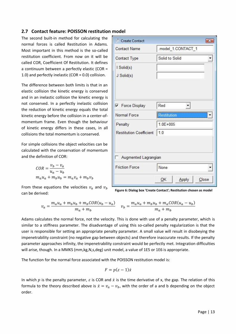
2.7 Contact feature: POISSON restitution model

The second built-in method for calculating the

normal forces is called Restitution in Adams.

Most important in this method is the so-called

restitution coefficient. From now on it will be

called COR, Coefficient Of Restitution. It defines

a continuum between a perfectly elastic (COR =

1.0) and perfectly inelastic (COR = 0.0) collision.

The difference between both limits is that in an

elastic collision the kinetic energy is conserved

and in an inelastic collision the kinetic energy is

not conserved. In a perfectly inelastic collision

the reduction of kinetic energy equals the total

kinetic energy before the collision in a center-of-

momentum frame. Even though the behaviour

of kinetic energy differs in these cases, in all

collisions the total momentum is conserved.

For simple collisions the object velocities can be

calculated with the conservation of momentum

and the definition of COR:

From these equations the velocities and

can be derived:

Adams calculates the normal force, not the velocity. This is done with use of a penalty parameter, which is

similar to a stiffness parameter. The disadvantage of using this so-called penalty regularization is that the

user is responsible for setting an appropriate penalty parameter. A small value will result in disobeying the

impenetrability constraint (no negative gap between objects) and therefore inaccurate results. If the penalty

parameter approaches infinity, the impenetrability constraint would be perfectly met. Integration difficulties

will arise, though. In a MMKS (mm,kg,N,s,deg) unit model, a value of 1E5 or 1E6 is appropriate.

The function for the normal force associated with the POISSON restitution model is:

In which is the penalty parameter, is COR and is the time derivative of x, the gap. The relation of this

formula to the theory described above is , with the order of a and b depending on the object

order.

Figure 6: Dialog box 'Create Contact'; Restitution chosen as model

Page | 14

2.8 Contact feature: Coulomb friction

Whereas the normal force is mandatory,

(Coulomb) friction is optional in the Adams

contact feature.

In Chapter 2.5 it was discussed that frictional

force (and coefficient of friction ) instantly jumps

from zero to a finite, non-zero value when the

relative velocity between the objects becomes

non-zero. Adams, however, does model this

discontinuity as a continuity, displayed in Figure 8.

When the value of the stiction transition velocity

( ) approaches zero, the closer the model

approaches stiction. However, Adams does not

allow , so it is impossible to model perfect

stiction.

The

function

follows cubic step functions from respectively

to , to and to . In

other intervals ( ) the coefficient of

friction is equal to .

The four characteristics ( ) are user-

specified in the dialog window. As said before, the

static and dynamic coefficients are often between

0 and 1. In Chapter 4, values for these coefficients

can be found for different contact materials.

These values are empirical. The dynamic

coefficient is typically lower than the static

coefficient, reflecting the common experience

that it is easier to keep something in motion

across a horizontal surface than to start it in

motion from rest. It is important to know that the

friction transition velocity ( ) is greater than the

stiction transition velocity ( ) by definition.

With the four user-specified values, Adams can

calculate coefficients of friction for every slip

velocity. This coefficient must be multiplied by the

normal force to determine the actual friction

force. So the choices made in the calculation of

the normal force are important for the calculation

of the friction force, too.

Figure 8 (bottom-right): Dialog box 'Create Contact'; Coulomb friction activated

Figure 7 (top-right): Representation of the coefficient of friction function

Page | 15

3. Cases:

3.1 Introduction

In this chapter a set of two models will be discussed. The first model considers a sphere bouncing on a fixed

box element that resembles the ground. With this model, the effect of all variables in both the IMPACT

function model and POISSON restitution model will be illustrated. The second model considers a sphere

rolling on top of a fixed box element. With this model, the effect of all variables in the Coulomb friction

model will be illustrated. Each case starts with a model description including a screenshot from Adams. The

two cases contain lists of observed effects when varying one variable. For each variable a list is included.

Both of these cases end with a discussion including explanations for observed phenomena.

At the end of this chapter we will have established an insight in the effects of all the variables associated

with the Adams contact feature.

Plotted graphs that are referred to in the cases can be found in Appendices A and B.

Page | 16

3.2 Bouncing ball (2D)

In the first case the behaviour of a sphere, with an infinite stiffness, falling onto a plane is observed. Since

the movement is purely vertical, friction plays no role and is turned off. To illustrate what the different

variables of the IMPACT function model and POISSON restitution model do, the Y-coordinate of the sphere’s

center-of-mass is analysed, which is initially 0.4 meters and collides with the floor at 0.0 meters.

First the IMPACT function model is researched and second the POISSON restitution model. The findings of

this research on both models will then be discussed in the last part of this case.

Figure 9: A sphere element (blue) falling and bouncing on a box element (brown)

Page | 17

3.2.1 IMPACT function:

Starting with a standard set of characteristics, the sphere’s behaviour is

discussed for different values of . By doing so, the effect of this

variable is illustrated. The time step used is 0.5ms, which appears

accurate enough for this purpose. The unit of stiffness is , force

exponent is dimensionless, the unit of damping is and that of

the penetration depth is .

In Appendix A, Figure 11, four different values of are plotted, one of them being the standard 2.2. In this

figure it can be seen that:

Low values of lead to rebounds and vibrations when the sphere is supposedly at rest.

At high values of , the sphere penetrates the floor, with increasing penetration depths.

There is an optimal at which no bouncing occurs.

To illustrate the effect of , the stiffness variable, several situations

with different values of are plotted. The standard set is as can be

seen be seen on the left, with a lower force exponent, . By doing so,

the effect of is more easily visible.

In Appendix A, Figure 12, four different values of are plotted. From the graphs it can be seen that:

At low values of , the sphere penetrates the floor, with increasing penetration depths.

Increasing leads to rebounds, with greater rebound heights for greater values of .

After an optimal the rebound heights decrease again until no rebound occurs anymore.

The effects of are plotted with the same low force exponent, , of

1.1. Four different values of are plotted, ranging from 1.0E+002 to

1.0E+005. The plots can be seen in Appendix A, Figure 13. From the

graphs it can be seen that:

Low values of allow relatively large rebound heights.

Increasing rapidly leads to complete suppression of the rebounds.

The last of the four variables is the penetration depth, . It is important

to note that this depth does not represent the maximum penetration

depth. It is the penetration depth at which the damping value is at

maximum. So it is in an important relation to the user-specified

damping value.

Appendix A, Figure 14, shows the behaviour for five different values of . From the graphs it can be seen

that:

Very small values for (1.0E-008 to 1.0E-004) show very little differences.

Increasing results in larger rebound heights, until a maximum is reached.

Page | 18

If damping is removed from the IMPACT function and the force

exponent is set to 1, the contact should be perfectly elastic. To

research this, the set of characteristics on the left was used and the

stiffness was varied. In the case of perfect elasticity, the sphere

would rebound up to 0.4 meters again.

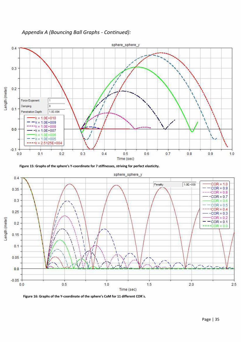
In Appendix A, Figure 15, the rebound heights are plotted for seven different stiffness values. From the

graphs it can be seen that:

High stiffness values lead to small rebound heights and small maximum penetration depths.

Low stiffness values lead to large rebound heights and large maximum penetration depths.

The rebound height converges to 0.4 meters.

The radius of the sphere determines the maximum penetration depth and thus the maximum

rebound height. Lower stiffness values cannot be researched with this model.

An easier way to achieve perfect elasticity is the POISSON restitution method. Before discussing the findings

above, the report continues with the POISSON restitution method.

Page | 19

3.2.2 POISSON restitution:

This method uses only two user-specified variables. First the value for

the penalty is kept static and the behaviour is evaluated for several

different values of COR (restitution coefficient). Then the value for COR

is kept static and the behaviour is evaluated for several different values

of , the penalty. The time step used here is also 0.5ms. The unit of penalty is and COR is

dimensionless.

In Appendix A, Figure 16, eleven different values of COR are plotted. In this figure it can be seen that:

COR = 1.0 does not lead to energy conservation, because is believed to be too low.

Decreasing the COR value leads to an increase of energy dissipation.

COR = 0.0 leads to 100% energy dissipation.

Now COR is kept static at 0.7 and the sphere’s behaviour is evaluated

for several different values for the penalty.

In Appendix A, Figure 17, ten different values of are plotted. In this

figure it can be seen that:

When is too low, the sphere sinks through the floor or the collision simply does not occur.

The higher is, the better the sphere follows the expected behaviour based on COR.

When is too high, an unexpected rebound can occur when the sphere is supposedly at rest.

The report will now continue with a discussion about all the findings above.

Page | 20

3.2.3 Discussion:

In the following paragraphs the findings from the previous pages are discussed. The order of the variables in

this discussion is the same as on the previous pages.

From the theory we know that the force exponent in the IMPACT function is a measure of the non-linearity

of the spring component. It is recommended to use values of . It was seen that values of

create unexpected vibrations, which is due to the relatively high spring force even at small penetration

depths. The recommended values of for rubbers, for soft metals and for harder

metals appear to be plausible. For high values, for example , the spring force is too small at small

penetration depths and thus the sphere will sink through the floor. It is recommended to use values

between 1.1 and 2.2, depending on the choice of materials.

On the subject of the stiffness we know from the theory that it is based on material and geometrical

properties. From the graphs it could be seen that when is too low, the spring force is insufficient to keep

the sphere from sinking. When is too high, the contact is obviously too stiff and the sphere will come to an

instant stop. It was also observed that there is an optimal value for . For this model is was

. The stiffness variable will be further researched in later cases.

The damping depends on two variables, the maximum damping variable, , and the penetration depth,

. A high maximum damping will lead to (almost) completely damped out rebounds. Decreasing allows

rebounds to occur. Decreasing even further allows larger rebound heights, until the rebound height

converges to a maximum at . The actual damping value ramps up from zero to over a distance

specified by . For high values of the rebounds appear to be less damped than in the case of low values of

. Especially when is larger than the actual maximum penetration depth, the work done by the damping

force is significantly smaller than for smaller values. When less work is done by the damping force, the

rebounds will appear less damped, which corresponds with the results in the graphs.

When the maximum damping is set to zero and the force exponent is set to one, the IMPACT function will

act as a linear spring. Perfect elasticity was expected, but it appears that a large penetration depth is needed

to achieve this. Since penetration depths should be relatively small in order for the model to be realistic, the

IMPACT function appears unsuitable for perfectly elastic contacts. The POISSON restitution model is

preferred for (near) perfectly elastic contacts.

The two user-specified variables in the POISSON restitution method are the COR (coefficient of restitution)

and the penalty. The COR is a measure of the energy conservation. According to the theory, the sphere

would rebound all the way up with a COR value of 1. This does not happen in the graph, because the penalty

value is not high enough. The higher the penalty value, the more accurate the rebounds are. This comes at

an expense, which can be seen in Figure 17 after . Suddenly unexpected rebounds can occur. This is

because the high penalty value can create large normal forces, even when the sphere is supposedly resting

on the floor. When the penalty value is far too low, the normal force cannot support the sphere at all. From

this it can be concluded that the POISSON restitution method requires the user to choose the penalty value

carefully.

Both normal force calculation methods have been evaluated and discussed in this case of the bouncing ball.

This case does not include frictional forces. These will be covered in the next case.

Page | 21

3.3 Rolling ball (2D)

In the second case the behaviour of a sphere, with an infinite stiffness, rolling on a plane is observed. Even

though the movement is purely horizontal, the normal force cannot be excluded. The frictional force

depends on the normal force. This case first researches the compatibility of several normal force options

with the Coulomb friction model. One specific option will be chosen with which the Coulomb friction model

will be researched.

To illustrate what the different variables of the Coulomb friction model do, the X-coordinate of the sphere’s

center-of-mass and its second derivative (the acceleration along the X axis) is analysed. From the theory it is

known that when there is no slip (meaning that there is no relative velocity between the sphere and the

floor), the frictional force is zero. A non-zero relative velocity produces a frictional force and so the sphere

will converge to a no-slip situation. Therefore the sphere is not given an initial translational velocity, but an

initial angular velocity. By doing so, the behaviour of the sphere can be observed while it converges to a no-

slip situation. The initial conditions are:

(the minus sign makes this rotation clockwise)

Figure 10: A sphere element (red) first slipping and then rolling on a box ement (green)

Page | 22

3.3.1 Suitable normal force configuration

Since the sphere is touching the floor throughout the whole simulation, a constant normal force is expected.

Oscillations in the normal force will affect the frictional force, as these oscillations will also occur in the

frictional force. So the criterion for the normal force configuration is that the resulting normal force is more

or less constant.

The IMPACT function acts as a mass-spring-damper system and calculates a normal force that is constant

when the sphere is in a vertical equilibrium at a specific penetration depth. Because of this, the Y-coordinate

of the sphere will oscillate at the start of the simulation and it will reach equilibrium after a period of time.

The length of this period depends on the user-specified variables in the IMPACT function and the time step

of the simulation. So the criterion is that the normal force is more or less constant before the relative

velocity nears the friction transition velocity.

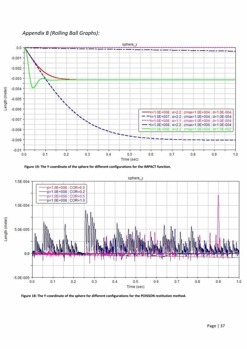
For several configurations of the IMPACT function, the Y-coordinate was plotted. The graph containing these

plots can be found in Appendix B, Figure 19. The time step used is 0.5ms. From the graph it can be seen that

lowering the force exponent, , to 1.1 provides us a normal force that appears to be suitable for this case, so

that the effect of the variables in the Coulomb friction model can be illustrated.

The POISSON restitution model is an alternative to the IMPACT function model, so it was also tested. In

Appendix B, Figure 18, it can be seen that the calculated normal force was far from constant. The plots of the

Y-coordinate are governed by vibrations, with COR=0.0 being an exception. This exception does lead to

discontinuities in the sphere’s acceleration and thus is not ideal for illustrating the Coulomb friction model’s

variables.

Upcoming research on the Coulomb friction model will be done with

the following normal force configuration:

Page | 23

3.3.2 Coulomb friction model

All the following simulations will be performed with the normal force

configuration stated on the previous page. Starting with a standard set of

characteristics, the sphere’s behaviour is discussed for different values of ,

the static coefficient. By doing so, the effect of this variable is illustrated. The

time step used is 0.5ms, which appears accurate enough for this purpose,

and is used throughout all the upcoming simulations in this model. The static

and dynamic coefficient are dimensionless and the transition velocities have the unit .

In Appendix B, Figure 21, the displacement in the X-direction is plotted for six different values of , one of

them being the standard 0.3. In this figure it can be seen that:

The parabolic start of the plots is the same for all values of .

The transition from the parabolic domain to the linear domain is differs per value of .

In all cases (except , which is an unrealistic value) the plots in the linear domain are parallel,

meaning that all values of lead to the same velocity in the X-direction.

In Appendix B, Figure 20, the acceleration in the X-direction is plotted for the same six different values of .

In this figure it can be seen that:

During the first milliseconds, the normal force approaches an equilibrium, creating vibrations in the

frictional force and thus acceleration. This also occurs in the other simulations of this model.

At first, the acceleration is constant and the same for all values of , hence the shared parabolic

domain in the previous graph.

When the contact point’s relative velocity decreases and reaches the friction transition velocity, the

acceleration increases to a maximum value that is . The duration of this increase is shorter

for higher values of .

After reaching a maximum, the acceleration quickly drops to zero.

The other efficient in Adams that is user-specified is the dynamic coefficient.

Starting with the same standard set of characteristics, the sphere’s

behaviour is discussed for different values of .

In Appendix B, Figure 23, the displacement in the X-direction is plotted for

five different values of , one of them being the standard 0.1. In this figure

it can be seen that:

The parabolic start of the plots differs for every different value of .

In all cases (except , which is an unrealistic value) the final velocity is the same.

never reaches the stiction transition velocity, since its initial friction force is zero and does

not change.

In Appendix B, Figure 22, the acceleration in the X-direction is plotted for the same five different values of

. In this figure it can be seen that:

At first, the acceleration is constant, but not the same for the different values of .

The constant acceleration is shorter for higher values of . Except for , which is a special

case since .

Page | 24

When the contact point’s relative velocity decreases and reaches the friction transition velocity, the

acceleration increases (or decreases for ) to a (maximum) value that is

. The duration of this increase is shorter for higher values of .

After reaching this maximum, the acceleration quickly drops to zero. The duration of this decrease is

the same for all values of .

Now that the coefficients have been researched, the transition velocities

remain. First the friction transition velocity, , will be varied while the other

variables have the same static values presented on the left of this text.

In Appendix B, Figure 25, the displacement in the X-direction is plotted for six

different values of . In this figure it can be seen that:

The parabolic start of the plots is the same for all values of , but extends further for lower values

of .

In all cases the plots in the linear domain are parallel, meaning that all values of lead to the same

velocity in the X-direction.

In Appendix B, Figure 24, the acceleration in the X-direction is plotted for the same six different values of .

In this figure it can be seen that:

At first, the acceleration is constant and the same for all values of . Lower values of have a

longer constant acceleration, hence the extended parabolic domain in the previous graph.

The maximum acceleration is the same for all values of , namely . The duration of the

increase towards this value is longer for higher values of .

The decrease from this maximum acceleration to zero is the same for all values of .

The other transition velocity is the stiction transition velocity, . In Appendix

B, Figure 27, the displacement in the X-direction is plotted for eight different

values of , including two values when . In this figure it can be seen

that:

When the parabolic domain is the same. When the parabolic domain is shorter.

Just like in the previous cases, the final velocity is the same for all values.

In Appendix B, Figure 26, the acceleration in the X-direction is plotted for the same eight different values of

. In this figure it can be seen that:

At first, the acceleration is constant and the same for all values of . The length of this constant

acceleration is the same for , but is shortened for .

All values lead to the maximum of . The duration of this ramp-up is shorter for higher values

of . When , this ramp-up is instanteous.

After reaching the maximum, all plots drop back to zero and share a common intersection point.

Only the graphs for do not share this common intersection point.

The report will now continue with a discussion about all the findings above.

Page | 25

3.3.3 Discussion:

In the following paragraphs the findings from the previous pages are discussed. The order of the variables in

this discussion is the same as on the previous pages.

When varying it was noticed that during the first 0.22 seconds the sphere’s behaviour was the same for

all values of , which is logical, because and are equal in all cases. It is when the relative contact

velocity drops below when the different cases start to act differently. Since , the sphere’s

acceleration is initially , and for different values of the acceleration increases (only

for , of course) to a peak value . Since is the same in all cases, these peaks are all at the

same velocity, . Then why do these peaks occur at different times? It is evident that the coefficient of

friction has a steeper incline for higher values of at a constant (review Figure 7 if this is unclear).

Therefore the frictional force increases faster for higher values of , decreasing the relative contact velocity

faster for higher values of and thus making the acceleration increase towards the spike steeper for higher

values of . And since the frictional force is higher at velocity for higher values of , the contact velocity

drops down to zero faster and so does the acceleration. When the acceleration has reached zero, the final

velocity is constant and the same for all values of . The parallel plots in Figure 21 show that the final

velocities are the same indeed. Values of lead to incorrect sphere behaviours according to the

theory of Chapter 2.8.

When varying it was noticed that the sphere’s acceleration starts at different values, which can be

explained by the simple fact that the acceleration is for contact velocities that are greater than ,

which is the case at the start of the simulation. Higher values of lead to higher frictional forces and thus

the velocity reaches earlier, at which the coefficient of friction starts changing from to . Since is

the same in all simulations, the sphere’s acceleration peaks at the same value. When , the change in

coefficient of friction is equal to zero. When the contact velocity remains constant and thus the

friction and stiction transition velocities are never reached. The change from to is shorter in time for

higher values of , because then the contact velocity is reached faster. After the peak, the acceleration

drops to zero at the same rate for all values of , since that rate depends on and only. Again the final

velocity is the same for all values of . When or the sphere’s acceleration is incorrect

according to the theory of Chapter 2.8.

When varying it was noticed again that the sphere’s acceleration is constant and the same for all

simulations. A higher value for means that the friction transition velocity is reached earlier, so the

increase in the acceleration starts earlier. All simulations have the same value for , which occurs at the

peaks of all plots. When the difference between these two transition velocities becomes smaller, the change

in acceleration becomes more rapidly, or even instant when . After the peak, the acceleration drops

down to zero at the same rate for all values of , since this rate only depends on and . Again the final

velocity is the same for all values of . When the sphere’s acceleration is incorrect according to the

theory of Chapter 2.8. In fact, cannot be modeled.

The last variable that was varied was . Since and are the same in all simulations, the acceleration is

the same at the start and at the peaks. When the acceleration instantly jumps to when the

contact velocity reaches . When the jump in the acceleration occurs earlier and the friction

transition velocity is completely disregarded. For values of that are greater than , which agrees with

the theory of Chapter 2.8, the difference between and determines the rate of climb from to .

Page | 26

Since the values of are different in the different simulations, the decrease from to zero is not the same

in all plots. Like in all other simulations, the final velocity is constant and the same for all values of .

The four sets of simulations show us several things. We now know how the sphere’s acceleration and

travelled distance are affected by varying the four variables , , and . Since the acceleration is

expected to be continuous, values for which a jump in the acceleration graph is created, are not

recommended. This excludes the values . The transition velocities are supposed to be non-zero:

. To follow the theory of Chapter 2.8, the coefficients of friction also have to be within a

certain range. The excluded values are: .

Page | 27

4. Recommended values:

4.1 Introduction

In Chapter 3 the variables of the IMPACT function model, the POISSON restitution model and Coulomb

friction model were analyzed and discussed with the use of two Adams models. Now that we know how

these models work and what effects the variables have on the contact behaviour, we want to know what

values are suitable for Adams models that resemble real-life constructions.

Chapter 4.2 will discuss the recommended values for the IMPACT function model, Chapter 4.3 will discuss

the recommended values for the POISSON restitution model and in Chapter 4.4 the recommended values for

the Coulomb friction model are discussed.

Page | 28

4.2 IMPACT function model

In this model there are four variables, namely stiffness , the force exponent , the maximum damping

and the penetration depth . These four parameters are discussed in this order in the following paragraphs.

4.2.1 Stiffness :

Even though the name stiffness might sound like it is a material property, it is not just that. It also depends

on the geometry of the colliding objects. Therefore there is no handbook for choosing the value for . The

best option is to do multiple simulations in Adams with different values of to determine the optimal value,

the value at which the Adams contact behaviour resembles the real world contact behaviour. Some

organizations that use Adams develop experience with the IMPACT function and its parameters, for their

specific applications.10

Since this study does not include extensive research like the aforementioned organizations do, we hardly

have any grip on what is a realistic value for the stiffness parameter. Adams includes a standard value for the

stiffness when initially setting up a contact between two objects, though. This value is .

Because of this, it is expected that a realistic value of would be in the range of to

.

4.2.2 Force exponent :

The force exponent is a measure of the non-linearity of the IMPACT function’s spring force. In Chapter 2.6 it

was already explained that the recommended value is , because lower values will lead to

discontinuities when IMPACT activates. The actual value of is a material property11. Soft materials, like

rubbers, have a force exponent of . For harder materials, the force exponent increases. Soft metals,

like aluminium, have a force a force exponent of and hard metals, like steel, have a force exponent

of . It is not recommended to use higher values, which was evaluated in Chapter 3.2.1.

4.2.3 Maximum damping :

Some sources say that it is recommended to have a maximum damping coefficient that is 1% of the stiffness

value12. Experienced users believe that should be even smaller. In Adams, the standard stiffness is

and the standard maximum damping coefficient is , which is 0.01% of the

stiffness value. The best option is to do multiple simulations in Adams with different values of to

determine the optimal value, the value at which the Adams contact behaviour resembles the real world

contact behaviour.

4.2.4 Penetration depth :

This penetration depth is not the maximum penetration depth, but the measure of how the damping

coefficient ramps up from zero to . The value should be smaller than the expected maximum

penetration depth. A reasonable value for this parameter is .13

To conclude Chapter 4.2: the IMPACT function works well as a method for calculating the normal force

during a collision, but determining the correct values can take extra research time, because of the geometry

dependency of the parameters.

10

Chris Verheul, ‘Contact Modeling’ presentation, sheet 10; http://www.insumma.nl/wp-content/uploads/SayField_Verheul_ADAMS_Contacts.pdf 11

Chris Verheul, ‘Contact Modeling’ presentation, sheet 11; http://www.insumma.nl/wp-content/uploads/SayField_Verheul_ADAMS_Contacts.pdf 12

Chris Verheul, ‘Contact Modeling’ presentation, sheet 13; http://www.insumma.nl/wp-content/uploads/SayField_Verheul_ADAMS_Contacts.pdf 13 Chris Verheul, ‘Contact Modeling’ presentation, sheet 12; http://www.insumma.nl/wp-content/uploads/SayField_Verheul_ADAMS_Contacts.pdf

Page | 29

4.3 POISSON restitution model

In this model there are two variables, namely the coefficient of restitution and the penalty

parameter . These two parameters are discussed in this order in the following paragraphs.

4.3.1 Coefficient of Restitution :

This parameter defines a continuum between a perfectly elastic (COR = 1.0) and perfectly inelastic (COR =

0.0) collision. These two perfect instances will never occur in real life, because the energy dissipation during

a collision will always be partial. In Appendix C, Table 1, a list of values for COR can be found. The table is

extracted from Adams/Solver documentation and lists 34 different combinations of materials. For each

combination a value for COR is given. In the table the values range from 0.65 to 0.95. When choosing the

POISSON restitution model, determining the correct value of the coefficient of restitution is fairly simple, by

using the table in Appendix C or different sources.

4.3.2 Penalty :

In the POISSON restitution model the COR is the most important parameter, but the penalty parameter

should not be forgotten. From Chapter 3.2.2 we learned how the penalty parameter affects the contact

behaviour. When the penalty is too low, the normal force is not sufficient. When the penalty is too high, the

normal force can become non-zero when it is expected to be zero, due to numerical integration issues.

Adams’ standard value for the penalty parameter is . Since integration issues are easily spotted

(note the random rebounds), the penalty can be increased until these integration issues arise. The most

preferred value for the penalty parameter is the highest value that does not cause integration issues.

To conclude Chapter 4.3: the POISSON restitution model is a great method for calculating the normal force

when the energy loss during a collision is known. The penalty parameter would have to be infinite for it to be

ideal, but that would lead to integration issues, too. Therefore, regardless of the value of COR, the penalty

parameter should be or greater if possible.

Page | 30

4.4 Coulomb friction model

In this model there are four variables, namely the two coefficients of friction, and , and the two

transition velocities, and . These four parameters are discussed in this order in the following

paragraphs. For reference it is advised to review Figure 7.

4.4.1 Coefficient of friction and :

When the contact velocity is between zero and the stiction transition velocity, the coefficient of friction

ramps up from zero to the static coefficient of friction . This coefficient is a material property, it depends

on the two materials of the objects in contact. For contact velocities between the stiction transition velocity

and the friction transition velocity, the coefficient of friction decreases from to , the dynamic

coefficient of friction. It is unusual for to be greater than , which can be seen in Appendix C. In that

appendix, in Table 1, and are listed for 34 different combinations of materials. In the table the values

are very wide-spread. So whenever an Adams model needs Coulomb friction to be implemented, the choice

of materials is very important, since it determines the static coefficient of friction and dynamic coefficient

of friction .

For both and the recommended values can be found by using the table in Appendix C or other sources.

If the specific combination of materials is not in the table, remember that when choosing your own

values.

4.4.2 Transition velocity and :

To determine what the recommended values are for both transition velocities and , we combine

knowledge from Chapters 2.5 and 2.8. In reality, the coefficient of friction instantly jumps from zero to at

contact velocity zero. This effect is known as stiction. Adams models this discontinuity as a continuity, seen

in Figure 7. Now the discontinuity at zero velocity is spread over a velocity range between zero and ,

making the coefficient of friction a continuous function of the contact velocity. Even though stiction is not

supported by Adams, the effect can be approached by making approach zero. The standard value in

Adams is . From Chapter 3.3.2 we know that this value can be increased, as long as its value remains

lower than .

When the contact velocity is equal to or greater than , the coefficient of friction remains constant at .

Like stated above, the friction transition velocity should be greater than the stiction transition velocity. The

standard value in Adams is .

In SolidWorks/COSMOSMotion14 the standard transition velocities for a contact between two dry steel

objects are and . This program uses a similar Coulomb friction model. When

comparing the standard values of Adams and the standard values of SolidWorks, it appears that the actual

choice for the transition velocities is very open to the end-user of the program.

To conclude Chapter 4.4: the Coulomb friction model is a great method for calculating the frictional force.

Even though stiction cannot be modeled, by choosing a low value for , the phenomenon of stiction can be

approached. The two known values of the coefficient of friction, and , are material properties and can

be found in Appendix C or other sources. The transition velocities are free to the user to choose, with

being close to zero and smaller than .

14 Kxcad, Understanding Contact Friction,

http://www.kxcad.net/solidworks/COSMOSMotion/usingmotionentities/constraints/contactconstraints/understanding_contact_friction.htm

Page | 31

5. Conclusion: In this study it was researched how the contact models in MSC Adams are derived from Hertzian contact

theory and other theories, how they are implemented in MSC Adams, what effect their parameters have on

the contact behaviour and what the recommended values are for these parameters.

The first contact method is the IMPACT function model. The IMPACT function creates a normal force that

consists of a spring force, which is derived from Hertzian contact theory, and a damping force, which is an

Adams addition. This method includes four user-specified parameters. Their effect on the contact behaviour

and the recommended values are discussed in Chapters 3.2.1, 3.2.3 and 4.2. The IMPACT function works well

as a method for calculating the normal force during a collision, but determining the correct values can take

extra research time, because of the geometry dependency of the parameters.

The second contact method is the POISSON restitution model. This method calculates a normal force based

on the coefficient of restitution and a penalty parameter. For every combination of two colliding materials

there is a certain value of the coefficient of restitution, which defines the energy loss during the collision.

COR = 1.0 means no energy is lost, COR 0.0 means all energy is lost. The effect of the two user-specified

parameters on the contact behaviour and the recommended values of these parameters are discussed in

Chapters 3.2.2, 3.2.3 and 4.3. The POISSON restitution model is a great method for calculating the normal

force when the energy loss during a collision is known. The penalty parameter would have to be infinite for it

to be ideal, but that would lead to integration issues, too. Therefore, regardless of the value of COR, the

penalty parameter as great as possible, without leading to integration issues.

The third contact method is the Coulomb friction model. This is a method for the optional frictional force.

Real-life friction also includes stiction, which is the frictional force when the contact velocity is zero. Adams

does not model this phenomenon. This method includes four user-specified parameters. Two of those, the

coefficients of friction, are material properties and can be found in tables. The other two parameters are

more open to the user to determine. The effect of the four parameters on the contact behaviour and the

recommended values of these parameters are discussed in Chapters 3.3.2, 3.3.3 and 4.4. The Coulomb

friction model is a great method for calculating the frictional force. Even though stiction cannot be modeled,

by choosing a low value for , the phenomenon of stiction can be approached. The two known values of the

coefficient of friction, and , are material properties and can be found in Appendix C or other sources.

The transition velocities are free to the user to choose, with being close to zero and smaller than .

Now that all three contact methods are discussed, we have a clear view of how they are to be used in Adams

models. In the next and last chapter recommendations will be made for further research in relation to MSC

Adams.

Page | 32

6. Recommendations: For further studies on the subject of contact in MSC Adams some recommendations are made:

To get a better insight in the parameters of the IMPACT function, it is recommended to build

physical models and model these in MSC Adams. By then comparing the Adams models with the

physical models, the ideal values for the parameters can be determined for these models.

From Chapter 3.3.2 we have seen that the rolling ball always ends with the same final velocity. So in

this case there is no rolling resistance. A research on rolling resistance in MSC Adams is

recommended. Taking a look into Adams/Car is a possibility.

Page | 33

Appendix A (Bouncing Ball Graphs):

Figure 11: Graphs of the Y-coordinate of the sphere's CoM for 4 different force exponents.

Figure 12: Graphs of the Y-coordinate of the sphere's CoM for 7 different stiffnesses.

Page | 34

Appendix A (Bouncing Ball Graphs - Continued):

Figure 13: Graphs of the Y-coordinate of the sphere’s CoM for 4 maximum dampings.

Figure 14: Graphs of the Y-coordinate of the sphere’s CoM for 5 different penetration depths.

Page | 35

Appendix A (Bouncing Ball Graphs - Continued):

Figure 15: Graphs of the sphere’s Y-coordinate for 7 stiffnesses, striving for perfect elasticity.

Figure 16: Graphs of the Y-coordinate of the sphere’s CoM for 11 different COR´s.

Page | 36

Appendix A (Bouncing Ball Graphs - Continued):

Figure 17: Graphs of the Y-coordinate of the sphere’s CoM for 10 different penalties.

Page | 37

Appendix B (Rolling Ball Graphs):

Figure 18: The Y-coordinate of the sphere for different configurations for the POISSON restitution method.

Figure 19: The Y-coordinate of the sphere for different configurations for the IMPACT function.

Page | 38

Appendix B (Rolling Ball Graphs - Continued):

Figure 20: The acceleration in the X-direction for different values of the static friction coefficient.

Figure 21: The X-coordinate of the sphere for different values of the static friction coefficient.

Page | 39

Appendix B (Rolling Ball Graphs - Continued):

Figure 22: The acceleration in the X-direction for different values of the dynamic friction coefficient.

Figure 23: The X-coordinate of the sphere for different values of the dynamic friction coefficient.

Page | 40

Appendix B (Rolling Ball Graphs - Continued):

Figure 24: The acceleration in the X-direction for different values of the friction transition velocity.

Figure 25: The X-coordinate of the sphere for different values of the friction transition velocity.

Page | 41

Appendix B (Rolling Ball Graphs - Continued):

Figure 27: The X-coordinate of the sphere for different values of the stiction transition velocity.

Figure 26: The acceleration in the X-direction for different values of the stiction transition velocity.

Page | 42

Appendix C (Material Contact Properties):

Material 1 Material 2

Dry steel Dry steel 0.70 0.57 0.80

Greasy steel Dry steel 0.23 0.16 0.90

Greasy steel Greasy steel 0.23 0.16 0.90

Dry aluminium Dry steel 0.70 0.50 0.85

Dry aluminium Greasy steel 0.23 0.16 0.85

Dry aluminium Dry aluminium 0.70 0.50 0.85

Greasy aluminium Dry steel 0.30 0.20 0.85

Greasy aluminium Greasy steel 0.23 0.16 0.85

Greasy aluminium Dry aluminium 0.30 0.20 0.85

Greasy aluminium Greasy aluminium 0.30 0.20 0.85

Acrylic Dry steel 0.20 0.15 0.70

Acrylic Greasy steel 0.20 0.15 0.70

Acrylic Dry aluminium 0.20 0.15 0.70

Acrylic Greasy aluminium 0.20 0.15 0.70

Acrylic Acrylic 0.20 0.15 0.70

Nylon Dry aluminium 0.10 0.06 0.70

Nylon Greasy aluminium 0.10 0.06 0.70

Nylon Acrylic 0.10 0.06 0.65

Nylon Nylon 0.10 0.06 0.70

Dry rubber Dry steel 0.80 0.76 0.95

Dry rubber Greasy steel 0.80 0.76 0.95

Dry rubber Dry aluminium 0.80 0.76 0.95

Dry rubber Greasy aluminium 0.80 0.76 0.95

Dry rubber Acrylic 0.80 0.76 0.95

Dry rubber Nylon 0.80 0.76 0.95

Dry rubber Dry rubber 0.80 0.76 0.95

Greasy rubber Dry steel 0.63 0.56 0.95

Greasy rubber Greasy steel 0.63 0.56 0.95

Greasy rubber Dry aluminium 0.63 0.56 0.95

Greasy rubber Greasy aluminium 0.63 0.56 0.95

Greasy rubber Acrylic 0.63 0.56 0.95

Greasy rubber Nylon 0.63 0.56 0.95

Greasy rubber Dry rubber 0.63 0.56 0.95

Greasy rubber Greasy rubber 0.63 0.56 0.95

Table 115

: Material contact properties; , and for X combinations of materials.

15 MSC Software, Adams/Solver help, p42/43; http://simcompanion.mscsoftware.com/infocenter/index?page=content&id=DOC9391