Bachelor Assignment Tactical Planning...
48
Bachelor Assignment Tactical Planning Efficiency How to improve the medium-term planning of Grolsch? Author: Rob Vromans Enschede, December 2011 Public
Transcript of Bachelor Assignment Tactical Planning...

Bachelor Assignment
Tactical Planning Efficiency How to improve the medium-term planning of Grolsch?
Author: Rob Vromans
Enschede, December 2011
Public

P.O. Box 55 7500AB Enschede
The Netherlands Brouwerslaan 1
7548XA Enschede The Netherlands
+31 (0)53 483 33 33 www.koninklijkegrolsch.nl
Grolsche Bierbrouwerij Nederland B.V. - A SABMILLER Company Correspondence address Head office Telephone Internet
Document Title
Status
Date
Author
Graduation Committee University of Twente
Grolsche Bierbrouwerij
How to improve the medium-term planning of Grolsch? Bachelor thesis for the bachelor program Industrial Engineering and Management at the University of Twente Public Report Bachelor Assignment 12-12-2011 Rob Vromans [email protected] +31 (0) 6 363 120 87 Dr.ir. J.M.J. Schutten School of Management and Governance Department of Operational Methods for Production and Logistics Drs. A. Roll Supply Chain Planning Manager Copyright © by R.F.M. Vromans. Public Thesis. All rights reserved. No part of this thesis may be published, copied or
sold without the written permission of the author.

Management Summary Tactical Planning of Grolsch is responsible for the medium to long-term planning of the filling
department. Two problems with Tactical Planning were identified by the supply chain planning (SCP)
department: the expected filling line efficiency of the planning is lower than the target for the actual
efficiency and the Tactical Planning is very sensitive to changes. Therefore, the main question of this
research is:
Which factors influence the medium-term planning
and how can Grolsch optimize the tactical planning strategy for the efficiency of production?
We identify 20 factors that influence the planned efficiency of production. From interviews with
planners, we determine that the forecast accuracy, demand volatility, and filling performance are the
main factors having a negative influence on the planned efficiency. Based on the description of
Tactical Planning, we find that Tactical Planning only influences the actual efficiency by the
determination of the number of setups per year in the Tactical Planning strategy.
Then we review scientific literature on improvement options and decide to calculate the impact on
cost that Tactical Planning has, through a cost calculation model. The cost calculation model
determines the lowest total costs of setups and holding stock per product family per filling line,
taking into account: demand, MTO/MTF products, safety stock, forecast accuracy, holding costs,
setup costs, minimum batch size, shelf life, and lead times. Finally we perform an experiment for the
entire filling department in which we compare the current strategy and actual number of setups to
the strategy for the lowest cost level.
Contrary to expectations, the outcome of this experiment shows that optimization for production
efficiency through decreasing the number of setups has no advantage at all because of the
interaction between the production and warehousing departments. By decreasing production
efficiency and increasing setups, Grolsch can either save money or redirect working capital.
We recommend Grolsch to focus more on the interaction between departments. SCP should refine
its knowledge of setup and holding costs and take these costs into consideration in its decision
making processes. First, in the decision to make a product on an MTO or MTF basis, we advise to aim
for more MTO products to reduce holdings costs. Second, the current planning strategy has proven
to be near to the optimal strategy. However, the belief that production efficiency improves the total
cost currently drives SCP to deviate from the Tactical Planning strategy. Because these deviations
have a negative impact on total costs, we strongly advise SCP to follow the Tactical Planning strategy
more strictly.
This thesis was limited to the production and warehousing departments only. Due to the unexpected
results of this research, we recommend SCP to further investigate the interaction between and
variable costs of these departments and eventually include the brewing department into the analysis,
to improve stability and costs of the total process.

Preface Does the improvement of production efficiency lead to cost savings? Production managers are
inclined to think it does, but in practice higher efficiency not always leads to savings in total costs of
the company. This research shows that this paradox is present at Grolsch, provides a model to
calculate the effect, and recommends on how to deal with it.
Of course, I could not have made this report without help. For the past five months, I did my research
at the Supply Chain Planning department of Grolsch, during which I worked as a logistical planner for
two months. This gave me the opportunity to experience Grolsch as a student and as an employee.
During my research, there was always someone to help me out when necessary, and many
colleagues have had the patience to answer my questions, provide information, and give feedback on
my proposals. I enjoyed working with such friendly colleagues. I therefore thank all colleagues at
Grolsch, especially my direct colleagues at Supply Chain Planning, who supported me.
During this research I had two supervisors. I thank Annelies Roll, my manager and supervisor at
Grolsch, who guided me through my research and always made time to discuss ideas and evaluate
my reports. Her expertise as well as her optimism were a constant encouragement and motivation.
Marco Schutten, my supervisor from the University of Twente, repeatedly gave me input and
feedback on my research plan and report. Thank you for your constructive evaluations and advice.
Finally, I thank my girlfriend Emma, my family, and friends for their continuous support.

Table of Contents List of abbreviations ................................................................................................................................ 1
Glossary ................................................................................................................................................... 1
1. Introduction ..................................................................................................................................... 3
1.1. Introduction Grolsch................................................................................................................ 3
1.2. Problem definition ................................................................................................................... 5
1.3. Problem statement and research questions ........................................................................... 7
2. Current situation ............................................................................................................................. 9
2.1. Tactical Planning process ........................................................................................................ 9
2.2. Planned efficiency ................................................................................................................. 11
3. Factors that influence the Tactical Planning ................................................................................. 13
3.1. Influencing factors on Tactical Planning ................................................................................ 13
3.2. Evaluation of the impact of influencing factors on planned efficiency ................................. 16
3.3. Conclusion ............................................................................................................................. 17
4. Improvement options for Tactical Planning .................................................................................. 18
4.1. Hierarchical planning framework .......................................................................................... 18
4.2. Tactical Planning of MTF products ........................................................................................ 19
4.3. Tactical Planning of MTO products ....................................................................................... 22
4.4. Conclusion ............................................................................................................................. 22
5. Theoretical and calculation model ................................................................................................ 23
5.1. Theoretical model ................................................................................................................. 23
5.2. Discussion of model ............................................................................................................... 27
5.3. Empirical research ................................................................................................................. 28
5.4. Conclusion ............................................................................................................................. 35
6. Conclusion and discussion ............................................................................................................. 36
6.1. Conclusion ............................................................................................................................. 36
6.2. Limitations and recommendations ....................................................................................... 37
6.3. Recommendations................................................................................................................. 37
7. References ..................................................................................................................................... 39
8. Appendices .................................................................................................................................... 40
Appendix 1: Model formulation ........................................................................................................ 40
Appendix 2: Tactical Planning Strategy Scenarios ............................................................................ 43

Page 1
List of abbreviations DP Demand Planning
ELSP Economic Lot Scheduling Problem
ERP Enterprise Resource Planning
FE Factory Efficiency
GBS Global Brewing Standards
HL Hectolitre
KPI Key Performance Indicator
MBS Minimum Batch Size
ME Machine Efficiency
MTF Make to Forecast
MTO Make to Order
RF Rolling Forecast
SCP Supply Chain Planning
SKU Stock Keeping Unit
SLA Service Level Agreement
TP Tactical Planning
WC Working Capital
Glossary Calculation model Mathematical formulation of theoretical model
Factory Efficiency A performance measure that states the effectiveness of a filling line
Factory Hours The number of hours that a line is operated during a week
Filling Line Production line on which beer is filled into bottles or cans.
Frozen window A frozen window is a period in which it is not allowed to make adjustments to a schedule or plan.
Global Brewing Standards The GBS contains rules that each SABMiller brewery must comply with. The goal of these documents is to set global rules in order to deliver beer with a constant high quality, independent of the brewery in which it is brewed.
Key Performance Indicator A measure that indicates the performance of a department/filling line or other entity of the company.
Lager beer Type of beer that needs to be filtered before it is filled.
Order lead time The order lead time is the time period in which Grolsch has to deliver the order to the customer.
Machine Efficiency A performance measure of the production department that states per line the availability of the line during the factory hours.
Make to Forecast (MTF) The make to forecast way of working is to keep a safety stock based on the forecasted orders. Customers can be delivered almost instantly.
Make to Order (MTO) The make to order way of working is to fill beer only based on actual orders.
Minimum Batch Size The Minimum Batch Size is an agreement that states the minimum volume of beer to produce per setup.
Model Simplified representation of reality that is constructed to

Page 2
study some aspects of that system.
Planned Efficiency The efficiency of a filling line would be executed exactly as the planning states.
Production Efficiency The efficiency of production.
Rolling Forecast (RF) A RF is a projection of demand into the future based on past performances, made by the Demand Planning.
SABMILLER SABMILLER is the owner of Grolsch and one the world’s largest brewers.
Service Level Agreement SLAs are contracts between a supplier and a customer of a certain service or product. It consists of agreements regarding the delivery, procedures, and the rights and obligations of both parties.
Setup A setup is a collection of actions that takes place when a filling line is adjusted to produce another product.
Maximum shelf life The maximum shelf life is the maximum number of weeks that beer may be in the finished goods warehouse before it is shipped to the customer.
Stock Keeping Unit A SKU is a unique identifier for every package and beer combination that can be ordered.
Tactical Planning (TP) TP is the medium term planning of SCP that determines when beer is produced.
Tactical Planning strategy The Tactical Planning strategy is a set of rules that TP follows when setting a Tactical Planning.
Working Capital Working Capital is the operating liquidity available to a business and the difference between short-term assets and short-term debt. An example of short-term assets is stock in the finished goods warehouse.
Young beer Young beer is beer that has just been brewed but has not matured yet.
Page 3
1. Introduction The planning department of Grolsch manages the timing and quantity of all material flows in the
brewery. Due to the uncertainty of many of these flows, the department is constantly synchronising
the schedules with all production and warehousing departments. This does not only lead to a high
workload on the department, but also to a lower efficiency of the brewery, due to constant
inefficient deviations from the previous schedule. The aim of this research is to find new options to
cope with the uncertainties in scheduling and optimize the planning, to increase availability and thus
output of the line. The exact nature of the uncertainties is unknown at the moment, requiring an
evaluation of the influencing factors before solutions can be sought.
This first chapter consists of the research plan: an introduction of Grolsch (Section 1.1) followed by a
description of the problem (Section 1.2), the problem statement (Section 1.3), and the research
questions (Section 1.4).
1.1. Introduction Grolsch
The introduction of Grolsch starts with a short outline of the history of Grolsch (Section 1.1.1) and a
brief description of the brewing (Section 1.1.2) and planning processes (Section 1.1.3), which helps to
understand the problem that Section 1.2 defines.
1.1.1. History of Grolsch
The research takes place at Royal Grolsch N.V., which is a daughter company of SABMILLER. Grolsch
was founded in 1615 in “Grol”. During the Second World War, a merger with a brewery from the
nearby city of Enschede took place. Grolsch was rewarded the royal title in 1995. In 2004, the new
brewery for Grolsch was completed in Enschede.
In February 2008, Grolsch was taken over by SABMILLER for around €814 million and became one of
SABMILLERs four global brands. As a result of this, the advanced Grolsch brewery now fills five
different brands of beer being Grolsch, Amsterdam, Miller, Tyskie, and Lech for the domestic market
(the Netherlands) and 70 export markets, including the United Kingdom, the United States, Canada,
France, and Poland.
1.1.2. Brewing process
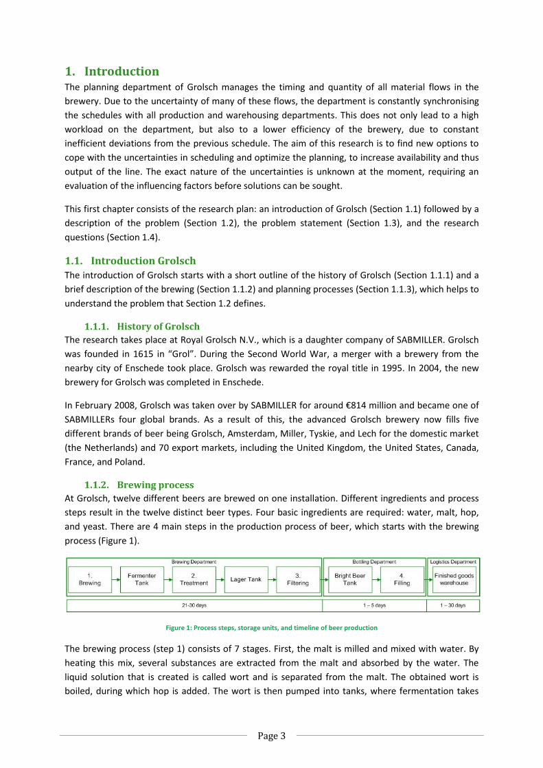
At Grolsch, twelve different beers are brewed on one installation. Different ingredients and process
steps result in the twelve distinct beer types. Four basic ingredients are required: water, malt, hop,
and yeast. There are 4 main steps in the production process of beer, which starts with the brewing
process (Figure 1).
Figure 1: Process steps, storage units, and timeline of beer production
The brewing process (step 1) consists of 7 stages. First, the malt is milled and mixed with water. By
heating this mix, several substances are extracted from the malt and absorbed by the water. The
liquid solution that is created is called wort and is separated from the malt. The obtained wort is
boiled, during which hop is added. The wort is then pumped into tanks, where fermentation takes

Page 4
place. To facilitate the fermentation, yeast is added. The yeast then converts the wort into ethanol
(alcohol) and carbon dioxide.
When fermentation is ready, most of the yeast is removed from the substance by means of
centrifuge, called treatment (step 2). The liquid is then pumped into lager tanks where it can mature
at a low temperature. After maturation, the beer is filtered (step 3) to exclude all yeast and other
turbidity-causing materials to stop the maturing process. This is done to stabilize the beer, which
means that there are no more visible changes. The filtered beer is stored in pressured Bright Beer
Tanks, from which it is pumped to a filling machine (or filler) at the filling lines. During filling (step 4)
the beer is put into cans, bottles or fusts and is packed into boxes or crates. The boxes and crates are
put on pallets and stored in the finished goods warehouse, from where they are transported directly
to customers or to SABMILLER warehouses.
1.1.3. Planning process
To align the brewing and filling departments, customer service, and warehouse departments, the
Supply Chain Planning (SCP) department was set up. SCP sets up Service Level Agreements (SLAs)
with customers to define what products can be ordered, the minimum quantity, order lead times,
the minimum shelf life the beer must have when shipped, storage conditions, shipping conditions,
the forecasts that the customer needs to deliver, and the order cancellation conditions.
The operational planning process starts with the accepted customer orders and sales forecasts, and
ends with the shipment of the orders. Forecasts are made by the Demand Planning (DP), which is
part of the commercial organization, and are combined with the orders per customer that are
grouped per Stock Keeping Unit (SKU), which is an unique identifier for every package and beer
combination that can be ordered. The planning department uses a hierarchical structure to manage
the rest of the planning process, as shown in Figure 2.
1.
Brewing
3.
Filtration
4.
Filling
2.
Treatment
Forecast by Demand Planning
Tactical Planning
Weekly
Brew planning
Daily
Packaging
schedule
Daily
Filtration schedule
Daily
Material call off
Service Level Agreements
Confirmed Orders
Figure 2: Planning process hierarchy
Page 5
The Tactical Planning (TP) uses the following information as input:
The agreed operating standards with the filling department
The stock policy
The confirmed orders
The forecasted demand
The stock in the finished goods warehouse
The required stock, determined from the demand for the first four weeks
The bottling capacity and the availability of materials
The already scheduled production for weeks 1 and 2
TP then makes a planning of bottling volume per SKU per week for 3 to 78 weeks ahead. The
planning is made per filling line per SKU by using a strategy that defines the production frequency.
The planning function of the SAP information system then initiates production orders on week level
to fulfil demand in time. The planning system does not take the maximum bottling capacity into
account when creating production orders. Therefore, a capacity check has to be done next. When
there is too much production in a certain week, the excess production is planned forward or
backward in time into a week with less production than the maximum capacity. Then the Tactical
Planning is used as an input for:
the weekly brew planning
daily packaging schedules
daily filtration schedules
daily material schedules
material forecasts
1.2. Problem definition
Because Grolsch has one of the newest and most advanced breweries in the world and highly trained
and experienced personnel, it has the potential to be one of the top breweries of SABMiller.
However, at the moment Grolsch is ranked around the 25th place in the SABMILLER benchmark of 78
breweries.
Since Grolsch has set itself the target to become top twenty this year and top ten next year, several
improvement plans have been started. In line with these projects, the planning department is
working to improve the Tactical Planning strategy with the aim to improve filling efficiency and to
reduce the uncertainties in the brewery. A first strategy was developed that defines the frequency
and timing of bottling runs. With this strategy variability in bottling volume per week and therefore in
brewing and filtration volume was reduced. The strategy also reduces outliers in filling volume and
thus acts as a peak shaving and smoothing instrument for the entire brewery. The aim of this
research is to scientifically investigate the steps already made and to find further improvements.
1.2.1. Targets
Being a part of SABMILLER, the Grolsch brewery is able to benchmark internally. The SABMILLER
Benchmark is a system that evaluates the performance of all SABMILLER Breweries against each
other to give insight in how individual breweries are performing. It includes many Key Performance
Indicators (KPIs), such as waste, efficiency, production quality assurance, and beer quality measures.
Page 6
For the operational organization, efficiency is the most important target because it is has a large
impact on the cost price and therefore influences the volume that SABMiller allocates to Grolsch.
SABMiller globally uses one set of standard KPIs with monthly and yearly targets. In addition
SABMiller works with a system in which the operational departments make ‘profit’ when they
perform better than budget and vice versa. Thus, continuous improvement is very important for
Grolsch.
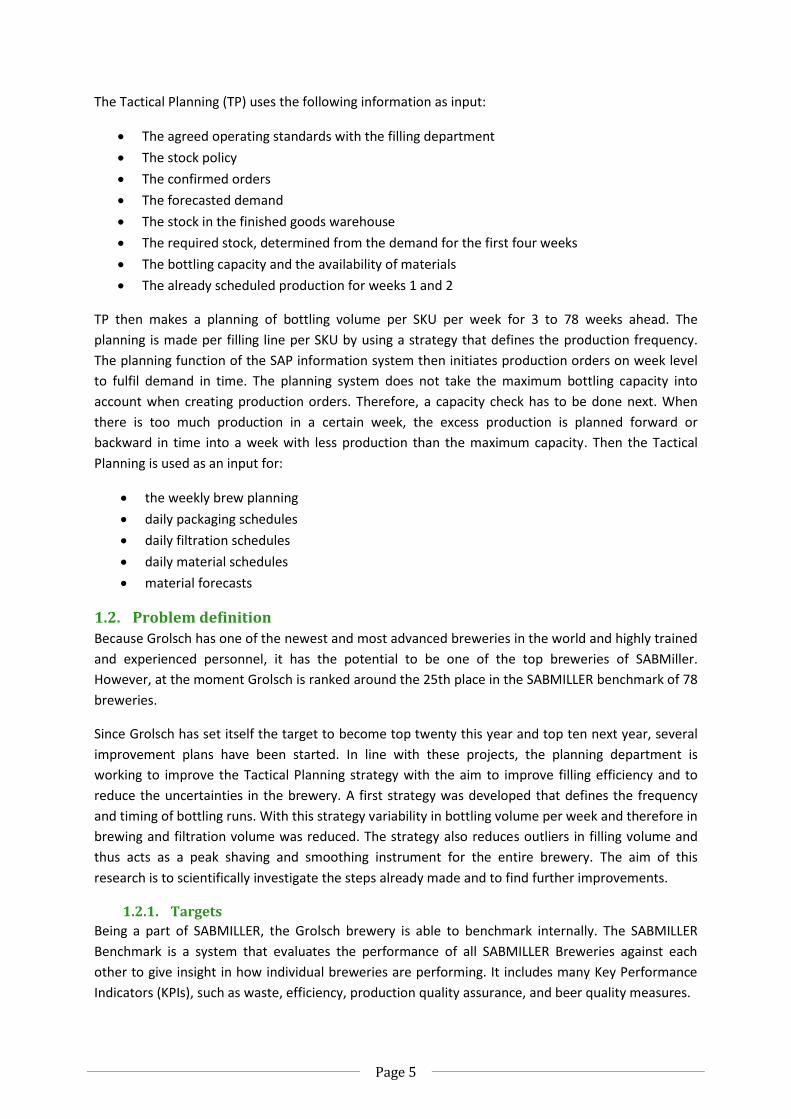
Grolsch uses two efficiency measures for production:
Machine Efficiency (ME) and Factory Efficiency (FE). ME
reflects the availability of a filling line: the time the filling line
actually fills related to the time personnel is present. FE
reflects the effectiveness of a filling line: the extent to which
the filling line has filled, according to its norm capacity. A
low efficiency ratio generally indicates an inefficient use of
resources and therefore a higher cost price per hectolitre of
beer. Figure 3 shows a visualization of the efficiency
measures and the differences between them. Planning has
an influence on the production efficiencies through the
efficiency of their plans, or Planned Efficiency.
All targets are collected per financial year that starts in April
and ends in March the following year. “F10 actual“ therefore
means the actual performance on a target between April
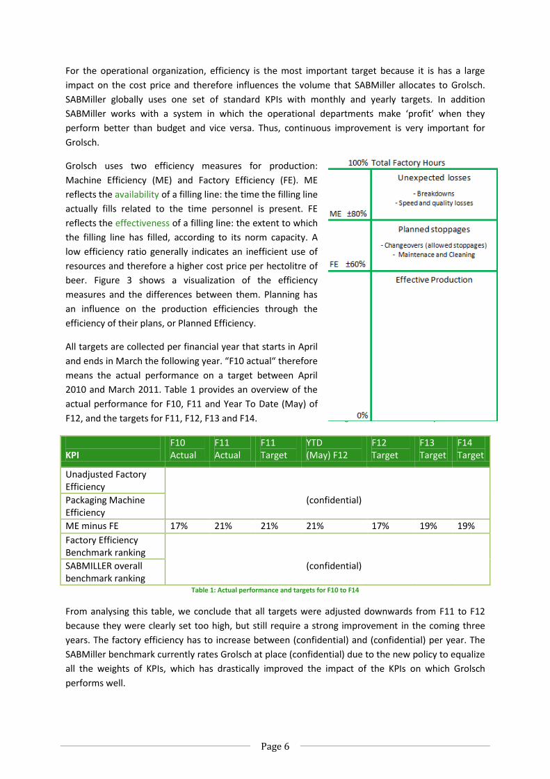
2010 and March 2011. Table 1 provides an overview of the
actual performance for F10, F11 and Year To Date (May) of
F12, and the targets for F11, F12, F13 and F14.
KPI
F10 Actual
F11 Actual
F11 Target
YTD (May) F12
F12 Target
F13 Target
F14 Target
Unadjusted Factory Efficiency
Packaging Machine Efficiency
(confidential)
ME minus FE 17% 21% 21% 21% 17% 19% 19%
Factory Efficiency Benchmark ranking
SABMILLER overall benchmark ranking
(confidential)
Table 1: Actual performance and targets for F10 to F14
From analysing this table, we conclude that all targets were adjusted downwards from F11 to F12
because they were clearly set too high, but still require a strong improvement in the coming three
years. The factory efficiency has to increase between (confidential) and (confidential) per year. The
SABMiller benchmark currently rates Grolsch at place (confidential) due to the new policy to equalize
all the weights of KPIs, which has drastically improved the impact of the KPIs on which Grolsch
performs well.
Figure 3: Overview of efficiency measures

Page 7
We therefore conclude that the operational departments of Grolsch need strong improvement,
evidently do not meet their targets, and that the pace of improvement is too slow. Part of this
improvement should be made by the planning department through improving their planned
efficiency.
1.3. Problem statement and research questions
The main problem for the Tactical Planning of Grolsch is the lack of a Tactical Planning strategy that
takes the most important influencing factors into account. The described problem leads to the
following problem statement:
Which factors influence the medium-term planning
and how can Grolsch optimize the tactical planning strategy for the efficiency of production?
This research is limited to the internal processes of Grolsch and assumes that the sales volatility,
forecast accuracy, production performance, material availability, and SLAs are fixed and known. The
objective of the research is to optimize the Tactical Planning process, to cope with the influencing
factors and diminish their influence on the planned efficiency. To find a solution to the described
problem, we use the following research questions.
1. What is the current planning process at Grolsch? (Chapter 2)
Chapter 2 describes and analyses the current planning process and the Tactical Planning at Grolsch in
detail. In particular it describes the information for and choices in the Tactical Planning and identifies
the restrictions. Furthermore, we describe the effect of the Tactical Planning on the efficiency of the
filling lines. We analyze internal documents such as agreements and documents on procedures, and
use interviews with experts when additional knowledge is required.
2. Which factors influence the medium-term planning and what is their impact? (Chapter 3)
Chapter 3 gives an overview of all influencing factors. The description and analysis of the process
helps to identify and fully understand the positive and negative factors, which is required to
determine the impact of the influencing factors. The chapter further provides an analysis of the
influencing factors on impact and the identification of the main problems.
3. What does literature describe about improvement options (Chapter 4)?
Chapter 4 is an overview of solutions to the problem found in scientific literature. It describes which
functions Tactical Planning should perform and elaborates on how we can determine the optimal
strategy for these functions.
4. What should Grolsch do to improve its performance? (Chapter 5)?
When it is clear what functions TP has and how we can determine the optimal strategy, we define a
model that is a simplified version of the reality and try to improve the Tactical Planning strategy by
using the model output. The insights and improvements from analysis of the model can then be
implemented in the TP.
Page 8
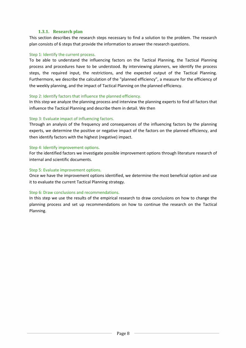
1.3.1. Research plan
This section describes the research steps necessary to find a solution to the problem. The research
plan consists of 6 steps that provide the information to answer the research questions.
Step 1: Identify the current process. To be able to understand the influencing factors on the Tactical Planning, the Tactical Planning
process and procedures have to be understood. By interviewing planners, we identify the process
steps, the required input, the restrictions, and the expected output of the Tactical Planning.
Furthermore, we describe the calculation of the "planned efficiency”, a measure for the efficiency of
the weekly planning, and the impact of Tactical Planning on the planned efficiency.
Step 2: Identify factors that influence the planned efficiency. In this step we analyze the planning process and interview the planning experts to find all factors that
influence the Tactical Planning and describe them in detail. We then
Step 3: Evaluate impact of influencing factors. Through an analysis of the frequency and consequences of the influencing factors by the planning
experts, we determine the positive or negative impact of the factors on the planned efficiency, and
then identify factors with the highest (negative) impact.
Step 4: Identify improvement options. For the identified factors we investigate possible improvement options through literature research of
internal and scientific documents.
Step 5: Evaluate improvement options. Once we have the improvement options identified, we determine the most beneficial option and use
it to evaluate the current Tactical Planning strategy.
Step 6: Draw conclusions and recommendations. In this step we use the results of the empirical research to draw conclusions on how to change the
planning process and set up recommendations on how to continue the research on the Tactical
Planning.
Page 9
2. Current situation This chapter extensively describes the Tactical Planning process. Chapter 1 described the role of
Tactical Planning in the planning process. The description of the TP process is necessary to
understand precisely what functions TP carries out and how it copes with the uncertainties in the
brewery. Section 2.1 describes the Tactical Planning and Section 2.2 explains how the quality of the
planning can be measured.
2.1. Tactical Planning process
The aim of the Tactical Planning process is to allocate resources to fulfil all orders within the
agreements made. Weeks 1 and 2 of a planning period are the frozen window, which is the period in
which in principle no adjustments in schedules are allowed. The tactical planner therefore focuses on
week 3 and further and only adjusts the planning for the first 2 weeks when major problems occur.
The Tactical Planning is made once a week, on Monday to ensure that the
information in the ERP system is accurate. Because the brewery is closed in
the weekend, on Monday all inventory numbers are exactly known. The
planned volumes of the week before have been communicated with the
scheduler who has accepted as many planned volumes as possible. The
volume that the scheduler has been able to schedule is then the planned
volume for week 2 of the frozen window. The accepted volume for weeks
1 and 2 is the first factor that is taken into account.
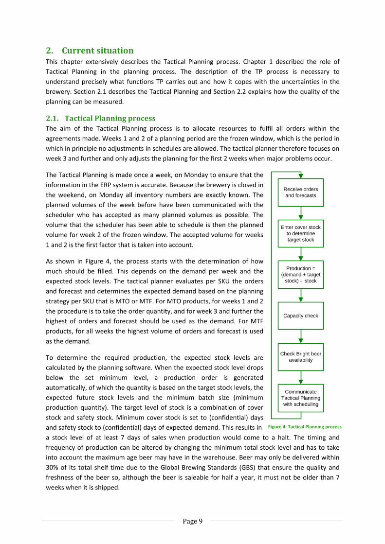
As shown in Figure 4, the process starts with the determination of how
much should be filled. This depends on the demand per week and the
expected stock levels. The tactical planner evaluates per SKU the orders
and forecast and determines the expected demand based on the planning
strategy per SKU that is MTO or MTF. For MTO products, for weeks 1 and 2
the procedure is to take the order quantity, and for week 3 and further the
highest of orders and forecast should be used as the demand. For MTF
products, for all weeks the highest volume of orders and forecast is used
as the demand.
To determine the required production, the expected stock levels are
calculated by the planning software. When the expected stock level drops
below the set minimum level, a production order is generated
automatically, of which the quantity is based on the target stock levels, the
expected future stock levels and the minimum batch size (minimum
production quantity). The target level of stock is a combination of cover
stock and safety stock. Minimum cover stock is set to (confidential) days
and safety stock to (confidential) days of expected demand. This results in
a stock level of at least 7 days of sales when production would come to a halt. The timing and
frequency of production can be altered by changing the minimum total stock level and has to take
into account the maximum age beer may have in the warehouse. Beer may only be delivered within
30% of its total shelf time due to the Global Brewing Standards (GBS) that ensure the quality and
freshness of the beer so, although the beer is saleable for half a year, it must not be older than 7
weeks when it is shipped.
Figure 4: Tactical Planning process
Receive orders
and forecasts
Enter cover stock
to determine
target stock
Production =
(demand + target
stock) - stock
Capacity check
Communicate
Tactical Planning
with scheduling
Check Bright beer
availability

Page 10
All planning steps are performed per SKU, and do not take the filling line capacity into account
directly. Therefore a capacity check is implemented that evaluates the planned production hours
against the number of hours that the filling lines are operational. The planned production hours
(hours that are required to fulfil all demand) depend on the operating standards and available hours.
When the operating standards are higher, for example the standard number of cans per hour
increases, the volume per week increases with an equal number of planned hours. When the
production is higher than the capacity, the capacity can be increased by using more shifts, or the
excess production can be brought forward or backward in time to weeks that have idle capacity, but
only when the delivery of orders is still guaranteed. When all of this is insufficient, Grolsch tries to
move orders in cooperation with the customers.
To determine how much (additional) volume can be filled, the available bright beer is evaluated (step
5 of Figure 4). The available bright beer depends on the brewing plan of four and more weeks earlier,
the actual time the brewing process took, and the moment at which young beer was treated into
lager beer. This results in an overview of lager beer available to be filtrated per day and the tactical
planner makes sure that the volume of required beer per week does not exceed the volume that is
available.
The last step in the TP process is to communicate the medium-term plan with the scheduler. The
scheduler gives feedback on the feasibility of the plan and uses the Tactical Planning as input for the
daily schedules.
2.1.1. Demand characteristics
The Tactical Planning receives the demand in the form of orders or production forecast. The forecast
is called Rolling Forecast (RF). The RF is based on the order history and includes the orders already
received, corrections for future circumstances such as weather, price elasticity, customer expansion,
penetration of the market, events and holidays, and introductions of for example seasonal beers
such as “Herfstbok”.
The customer orders that Tactical Planning receives are all orders that are checked and accepted by
both Grolsch and the customer. Requests for orders within the frozen window that are outside the
forecast are directly sent to the scheduler, who decides whether the extra demand can be met based
on availability of beer, capacity, and materials. For the tactical planner, the RF has two important
dimensions: how volatile the demand in the forecast is and how accurate the demand is forecasted.
Demand volatility Demand volatility is the degree of change between the total volume of demand between weeks. The
changes in demand are important for the tactical planner because they are reflected in the capacity
that is required per week. If there is little stock capacity, the filling line has to follow the changing
demand with fluctuating production levels. Further, a volatile demand results in higher peaks and can
therefore result in problematic warehouse occupation and manning availability.
Page 11
Forecast Accuracy The accuracy of the forecast is even more important. When the actual demand is higher than
forecasted, extra and smaller production orders have to be issued to meet the orders. When the
volume for a month is accurate but the timing in weeks is off, stock can be piling up in the
warehouse, or beer has to be packaged earlier than expected which again leads to rushed
production.
2.1.2. Cover stock strategy
To improve the efficiency of the filling lines and reduce the number of setups, from a planning point
of view the main instrument is to enlarge batch sizes. When production runs are longer, less setups
are required which results in more cans filled per hour. To increase batch sizes, the tactical planner
determines a production frequency per product family of once every one, two, or four weeks. A
product family is a group of SKUs with the same beer type. SKUs are grouped because a change
between beer types requires a bigger setup than changes in packages or labels. By grouping the SKUs
into families, the goal is to produce all SKUs with the same beer type in one batch. It does however
result in a restriction on flexibility for separate SKUs: if a family is filled once every month, it is very
costly for one SKU to be filled twice every month, because an extra family setup (beer type change) is
required.
The strategy is implemented in the planning by adjusting the cover stock levels per SKU in SAP, a
time-consuming process. For example, when a product has a low volume and can be made once
every four weeks without resulting in too much stock, the cover stock for week 1 is set to 28 days, for
week 2 to 21 days, for week 3 to 14 days, and for week 4 to 7 days. The planning program then
returns a production order in week 1 for the total demand for the coming four weeks, making sure
that in week 2, 3, and 4 there is also enough stock.
2.1.3. Restrictions on TP
Next to the bright beer availability that TP checks directly, other restrictions are indirectly taken into
account by TP. The GBS lead to limitations in the brewing department and limit the available bright
beer. The order lead times defined in the SLAs are reflected in the accepted orders per week and the
agreed operating standards limit the capacity of the filling lines.
The limited warehouse capacity is another restriction on production that is not taken into account.
Currently, when orders increase or batch sizes are increased, warehouse capacity is not taken into
account by the tactical planner, because it is only occasionally found to be a real restriction.
2.2. Planned efficiency
The process described in Section 2.1 leads to a Tactical Planning that states the timing and size of
production batches per SKU. All weeks of production orders are then sent to the scheduler, who
schedules them per filling line in time and in full detail for the first two weeks. The schedule that
follows from this process is evaluated each week to calculate the planned efficiency per week. The
planned factory efficiency per week is found by the following calculation.

Page 12
The denumerator of the main fraction is the planned volume divided by the maximum volume per
hour per SKU that a filling line can fill. This means that per SKU the volume is divided by the
maximum production speed of 72000 cans per hour to find the time that it could and thus should
take to fill this volume. Furthermore, the planned factory hours are the total hours that the filling line
is manned during the week. When the filling line is able to fill the volume scheduled in a week in 70
hours of filling and the factory is operating 100 hours, the planned factory efficiency is 70%. The 30%
fraction that is not in the planned FE is the time that is planned for setups, maintenance and
cleaning, and speed losses.
2.2.1. Impact of Tactical Planning on planned efficiency
The tactical planner determines the planned volume per SKU per week and is thus able to influence
the planned efficiency. However, the planned volume is restricted by the filling line capacity that is
agreed between the filling department and the planning department. The capacity is based on the
operating standards that define how much speed losses the planning department has to take into
consideration to make a feasible and realistic schedule. It is up to the operating standards to ensure
that the gap between planned efficiency and actual efficiency is as small as possible.
The planned volume is further restricted by all other time losses through setups and M&C
(maintenance & cleaning) stops. M&C stops are imposed by the GBS (global brewing standards) and
are only influenced by the scheduler who can sometimes plan the M&C stops during setups.
Therefore Tactical Planning can only influence the efficiency by the determining the number of
setups. The number of setups depends on the number and composition of SKUs that are planned per
week. By planning less SKUs per week, the number and thus the total duration of setups is reduced
which leaves more time for production, increasing planned volume and thus efficiency.

Page 13
3. Factors that influence the Tactical Planning This chapter identifies and describes the factors that influence the input and output of the Tactical
Planning (Section 3.1). Section 3.2 evaluates the impact of the factors and determines which factors
are interesting for further research. Section 3.3 presents a conclusion on the impact of the
influencing factors.
3.1. Influencing factors on Tactical Planning
The influencing factors can be divided into four categories of direct factors based on their
characteristics, being: Input of planning, Actual past performance, Strategic factors, and Constraints
on the planning. Furthermore, some identified factors influence the factors in the four categories and
thus influence the planned efficiency indirectly. Figure 5 shows the four direct categories and the
indirect factors to visualize the relations between the influences. The following sections describe how
the factors influence the planning in practice.
Figure 5: Factors that influence the Tactical Planning.
3.1.1. Information input
For Tactical Planning the most important information is the demand forecast, so together with the
agreed operating standards and actual current stock the expected stock can be calculated per week.
The demand forecast is made by Demand Planning (see Chapter 2).
3.1.2. Actual situation
Another part of the required information is the actual performance of the production department,
which is reflected in the changes in the schedule that have been made since the last Tactical Planning
and the resulting finished goods stock in the warehouse.
Incidents that lead to weekly volume changes Malfunctions, breakdowns, lost time due to material unavailability or deviations from schedules in
production, lead to changes in the daily schedules. When these changes are too big to be solved
during the week and result in volume that is passed on to the next week, they influence the Tactical
Planning.
Orders- Sales volatility
- Forecast accuracy
Planned
Efficiency
Constraints- Canning line capacity
- Warehouse capacity
- GBS
Material
availability- Bright beer
- Packaging materials
Actual- Deviating daily
schedule
- Finished goods stock
Strategy- Production strategy
- TP strategy
Performance- Adherence to schedule
- Unplanned downtime
SLAs+ Order lead times
+ Minimal batch size
- Maximum age
Input- Demand Forecast
- Expected stock
- Expected performance
Planned downtime- Planned stops
- New product developm.

Page 14
Actual finished goods stock The actual finished goods stock is one of the main inputs and is a result of filling performance and
actual sales. To guarantee a 99% service level as agreed in the SLAs, Grolsch has a stock policy that
must be met by the tactical planner to cope with the uncertainties of production and demand
(minimum cover stock of two days and a safety stock of five days). When the cover stock drops below
seven days, a production order is planned.
Orders The actual finished goods stock is a result of the actual sales and production. Next to the actual sales,
also the ‘Forecasted Sales’ influence the Tactical Planning.
Random Demand / Forecast accuracy: the Tactical Planning receives demand in the form of orders
and the rolling forecast (RF), including orders and expectations from now until week 78. The forecast
is accurate for about 72%. This means that on average 28% of the volume per SKU is changed before
or during actual production. More or less orders within forecast: the forecast can be changed for
week 3 until week 78 with additional or less volume due to new or stopped orders from existing
customers, new or leaving customers, other volumes allocated by SABMiller, products that are
brought to or are taken off the market, disappointing market results etc. Orders outside Forecast:
when orders are changed, aborted, or require rushed delivery within 2 weeks, the customer services
department pushes a rush order request to the scheduler. The scheduler investigates all possibilities
and accepts or rejects the request. This results in more volume for the first two weeks and maybe
less volume for later weeks.
Material availability It is very problematic when the glass supplier cannot meet the demand for bottles, the agricultural
supplier cannot send enough malt, hop, or sugar, or the brewing department has not enough beer
available. Furthermore, due to a focus on Just in Time (JIT) delivery, the raw material warehouse is
only capable of containing 24 hours of stock and thus problems arise when production does not use
the received materials within 24 hours and when suppliers are too early with their deliveries.
Bright beer availability Tactical Planning plans beer volume per week and makes sure enough bright beer is available. When
bright beer turns out not to be available in time for the filling line, this results in schedule changes
and it can also lead to shifts in volume between weeks, which effects the Tactical Planning.
Filtration performance: one of the causes for unavailability of bright beer is the filtration
performance. During filtration, lager beer is pushed through a filter to remove all yeast and turbidity-
causing materials. Filtration generally falls back on schedule when filtration run lengths are shorter
than expected. Every new filtration run results in two hours of setup time. When filtration is not on
schedule, the beer is not available in time for the filling line. Bright beer quality: if the laboratory
tests that analyze the quality of the beer indicate a too high or low value for brightness, colour, foam
quality or bitterness, the beer is disapproved and requires rework, has to be filled together with beer
of good quality or in the worst case has to be flushed down the drain. Especially the unavailability
during rework causes long delays.
Page 15
3.1.3. Strategy
The required demand based on the demand forecast and actual stock, is then transformed into a
production planning by using a planning strategy. Section 2.1.2 describes the use of the planning
strategy and Appendix 1 states the current strategy as of august 2011.
3.1.4. Constraints
Because the tactical planner faces limited warehouse capacity, filling capacity, and bright beer
availability, the number of options for a feasible planning is limited. We therefore now describe
which constraints TP has to deal with.
Filling line capacity The filling lines have a certain maximum capacity which depends on the line capacity and the
manning. The line capacity depends on the filler speed, the volume per can (the filler can fill
(confidential) cans per hour, that is (confidential) Hl when 50cl cans are used and (confidential) Hl for
33cl cans), the required M&C and setups as described in Chapter 2, and the available personnel or
manning. Filling lines have to be operated by skilled personnel, and the capacity depends on the
number of scheduled shifts. Because some lines share personnel, their capacity depends on the
allocation of shifts per line.
Warehouse capacity The Grolsch brewery has a warehouse that is built for make-to-order products that are stored at
most for 48 hours. Since Grolsch fills some beer types on a make-to-forecast strategy only once in a
month, the warehouse is filling up and the capacity may become a constraint for Tactical Planning.
The target level and actual amount of safety stock influence planned efficiency because it decreases
the warehouse capacity that is available for production. There is less safety stock required when
forecast accuracy is increased, the required service level is decreased, or products are made MTO
instead of MTF. With less safety stock and thus more room for normal stock, batch sizes can be
increased which has a positive effect on efficiency.
Brewing capacity The Grolsch brewery has two brewing lines; each can brew (confidential) brewages or (confidential)
Hl per week. Grolsch uses only one brewing line during low season but in peak season the second is
used as well. The capacity is limited to (confidential) Hl as long as the revenues for the second line
are not exceeding the extra setup and energy costs.
SLAs SLAs are the agreements with internal SABMILLER commercial organizations per stock keeping unit
that include the negotiated order lead times, minimal batch sizes, brewing standards, minimal shelf
times, and if applicable the months in which the product can be ordered.
Order lead times: SLAs determine the time between the acceptance and delivery of orders, the order
lead times. The tactical planner has to meet these agreements, also when these agreements are set
too tight. Longer lead times mean more time and therefore more flexibility for the production of the
order. Minimal Batch Size: SLAs further determine the minimal size for orders and the minimal
amount of orders that are required to start production. This is positive for the tactical planner when
the sizes are sufficient because this results in less and bigger production batches. Global brewing
standards: the GBS are standards for the production of beer that determine for example the minimal
Page 16
or maximum residence time and volume of beer in young beer or bright beer tanks. Maximum age /
Minimal shelf time: the agreements on minimal shelf time determine that the beer that is delivered
to the customer has a certain shelf time left. This limits the last possible production date when the
delivery date is certain. SKUs with small quantities per month therefore lead to monthly small
batches, because the finished product would be too old when this product would be filled every half
year in a much bigger batch.
Planned Downtime Planned maintenances: Tactical Planning has to take into account the efficiency lost on the filling line
due to planned maintenances and cleaning stops. Product testing or product phase out: Grolsch
regularly introduces new labels on bottles and sporadically starts with a new beer type or brand.
These new labels, bottles or beer types are tested first with a number of small batches that require a
long first time set up and cost a lot of time and efficiency. There are also products that are phased
out of production and require a small batch to meet the last demand.
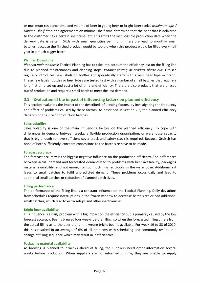
3.2. Evaluation of the impact of influencing factors on planned efficiency
This section evaluates the impact of the described influencing factors, by investigating the frequency
and effect of problems caused by these factors. As described in Section 2.3, the planned efficiency
depends on the size of production batches.
Sales volatility Sales volatility is one of the main influencing factors on the planned efficiency. To cope with
differences in demand between weeks, a flexible production organization, or warehouse capacity
that is big enough to have sufficient cover stock and safety stock is required. Because Grolsch has
none of both sufficiently, constant concessions to the batch size have to be made.
Forecast accuracy The forecast accuracy is the biggest negative influence on the production efficiency. The differences
between actual demand and forecasted demand lead to problems with beer availability, packaging
material availability, and not enough or too much finished goods in the warehouse. Additionally it
leads to small batches to fulfil unpredicted demand. These problems occur daily and lead to
additional small batches or reduction of planned batch sizes.
Filling performance The performance of the filling line is a constant influence on the Tactical Planning. Daily deviations
from schedules require interruptions in the frozen window to decrease batch sizes or add additional
small batches, which lead to extra setups and other inefficiencies.
Bright beer availability This influence is a daily problem with a big impact on the efficiency but is primarily caused by the low
forecast accuracy. Beer is brewed four weeks before filling, so when the forecasted filling differs from
the actual filling as to the beer brand, the wrong bright beer is available. For week 19 to 33 of 2010,
this has resulted in an average of 6% of all problems with scheduling and commonly results in a
change of filling sequence which may result in inefficiencies.
Packaging material availability As brewing is planned four weeks ahead of filling, the suppliers need order information several
weeks before production. When suppliers are not informed in time, they are unable to supply

Page 17
Grolsch with the necessary materials. This influence is therefore another result of the low forecast
accuracy. Besides, another problem is the supplier reliability. The impact of these two factors is
estimated to be very low due to the fact that currently only an average of 2.5% of all problems that
scheduling faces are caused by material unavailability. Because scheduling most often copes with
these problems within the same week, the effect on the Tactical Planning is estimated to be less than
1%.
New product development The influence of the testing of new products, and of small batches of products that are phased out, is
very low compared to the daily problems. The projects are planned in advance and lead to some
inefficient small batches but not to changes in the planning.
Order lead times and minimum batch size The agreed order lead times and MBS (minimum batch size) have a positive influence on the Tactical
Planning. Order lead times limit the possible interruptions of customers on the daily schedules and
the MBS enlarges the average batch size.
Maximum age and warehouse capacity The maximum age and warehouse capacity are both a restriction on batch sizes. Because batch sizes
are currently lower than possible, these restrictions are not taken into account. When batch sizes
increase, these restrictions will become important factors.
Filling line capacity The filling lines are currently operated 104 to 112 hours per week. Because lines are stopped in the
weekend, much cleaning time is lost on Friday and setup time is necessary on Monday. With the
weekend as back-up capacity, and an estimated 22% of idle time (mainly in low season) for the next
year, the filling line capacity is currently no restriction for the planned efficiency.
Global brewing standards The global brewing standards have an indirect impact on efficiency. The standards put a restriction
on the full capacity usage of lager beer tanks which leads to bright beer availability problems.
3.3. Conclusion
We identify 20 factors that influence the Tactical Planning and thus the planned efficiency. After
evaluating all influencing factors, we conclude that the low forecast accuracy, high demand volatility,
and unreliable filling performance are the main negative factors on the planned efficiency. We
further expect that the maximum age and warehouse capacity will gain more influence when batch
sizes are increased.

Page 18
4. Improvement options for Tactical Planning This chapter investigates options for improvement of Tactical Planning to cope with the negative
factors. Section 4.1 analyses the hierarchical structure and division of planning tasks within the
planning department and describes the selected functions for the Tactical Planning. Sections 4.2 and
4.3 provide methods and procedures found in literature.
Readers who are not interested in the literature review can skip to Chapter 5 and readers who are
not interested in the model itself can skip to Section 5.4.
4.1. Hierarchical planning framework
Grolsch uses a planning process hierarchy as described in Chapter 1 to tackle the complex and
extensive planning process. The use of a production planning hierarchy is supported by the
operations research literature. Hierarchies found in literature usually have in common that they work
with three levels: the “strategic” (long-term), “tactical” (intermediate term), and “operational or
control” (short-term) level. The levels that these hierarchies show are meant to have the following
effects: decisions made in earlier phases of the planning process, or higher levels create boundaries
for the decisions in later phases. In line with this there are more decisions to make on the
operational level than on the strategic level and more adjustments needed. This is due to the fact
that lower level activities are performed more closely to the actual production and thus have more
information available. Important for these hierarchies to make things work is feedback to ensure
consistency and learning.
Figure 6 gives a planning hierarchy by Soman et al. (2004), presenting a more elaborate hierarchy,
that fits with Grolsch because it is developed for the combined MTO and MTF planning in food
industries. It focuses on the planning function and makes a distinction between choices made per
phase based on the concept of “frequency separation”. To use this concept, first the frequency is
determined for all decisions and then decisions are allocated to hierarchy levels by frequency. The
more frequent decisions should be made during lower level activities and vice versa.
Figure 6
Strategic long-term
Tactical medium-term
Operational short-term
Figure 7 Planning hierarchy for MTO/MTF (Soman et al. 2004)

Page 19
Next to feedback within the planning department, the framework presented by Soman et al. includes
the check on production performance that creates feedback to all phases in decision making. The
hierarchy level names can again be assigned to the steps in the framework. This research considers
the medium term capacity co-ordination because it resembles the tactical function of Grolsch. Soman
et al. states that the function of Tactical Planning is to balance demand and capacity. Tactical
Planning should allocate production orders to planning periods based on actual orders, forecasts,
available capacities, stocks and realized efficiencies. Furthermore, TP should specify the target level
inventory for MTF products and set a policy for order acceptance and due dates for MTO products.
Per production order, the production run length and cycle length should be specified. We now follow
Somans recommendations and search for literature on how to perform the tasks assigned to TP,
separately for MTO and MTF products.
4.2. Tactical Planning of MTF products
The Tactical Planning is closely related to inventory management due to the fact that the number of
setups has an effect on batch sizes and thus have an effect on the average amount of stock in the
warehouse. According to Hopp and Spearman (2008), the first theory to determine batch sizes and
corresponding production frequencies in the stock management literature was based on the
Economic Order Quantity formula by Harris (1913) that is used to make a trade-off between holding
costs and setup costs.
With as batch size, as setup cost per setup, as holding cost per product, and as demand
rate. The assumptions under which this formula creates an accurate output are:
Constant and known demand
One line, one product and no product interactions
Instant production
No lost sales, backlogging possible
Constant and known costs of setups
Constant and known costs of holding stock
The EOQ is the most famous function for batch sizes and is very easy to understand and apply. The
problem with this formula is the high number of unrealistic assumptions. To be able to use the
concept some alterations have to be made. Taft (1918) made an extension called Economic
Production Lot (EPL) for production which is not instantaneous:
where is the production rate. Because the EPL works only with the setup and holding costs of one
product and can thus determine that the optimal situation requires more setups or stock than
possible, a model is required that also makes a trade-off between products. Therefore we first need a
Page 20
total cost function for all products considered. Because setup costs and holding costs depend on the
batch size the total cost function can be written as:
where is the total cost of the setups and keeping stock, the cost of a setup and
the cost of keeping one unit of stock. Now we can minimize the total cost function for several
products with the Multiproduct EOQ model as proposed by Hopp and Spearman (2008). As an
example they give a model that minimizes the inventory costs for a problem with multiple products
with the formula:
Where is the cost of holding inventory of, and is the batch size of product . This can be
expanded with other holding costs and setup costs to create a total cost model.
This model does however not include the stochastic behaviour of demand. When Grolsch has no
stock to fulfil demand and the product is not scheduled for production on time, the revenue is lost.
Therefore, we need a multiproduct model that includes the forecast accuracy and the costs of stock
outs that are related to it. The Multiproduct (Q,r) Stockout Model from Hopp and Spearman (2008)
takes this into account by minimizing the inventory holding cost, subject to the constraint that the
average fill rate (or service level) must be above an agreed level. The model determines the optimal
batch size with the EOQ model and the reorder level by using the standard deviation and mean of the
time it takes to order or produce the product. This implicates that the stochastic problem of forecast
accuracy can be made deterministically by setting a reorder level in stock management that copes
with the uncertainty.
Because Grolsch does not order products but produces them, the reorder level is replaced by safety
stock that is kept in the warehouse. We thus need a multiproduct model that minimizes total costs
for production (setups) and stock management and takes the safety stock into account to adjust for
forecast accuracy.
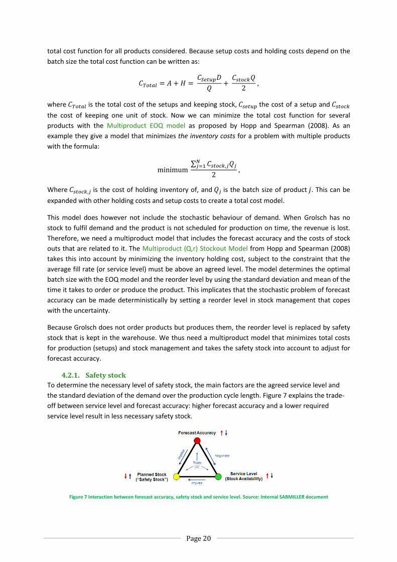
4.2.1. Safety stock
To determine the necessary level of safety stock, the main factors are the agreed service level and
the standard deviation of the demand over the production cycle length. Figure 7 explains the trade-
off between service level and forecast accuracy: higher forecast accuracy and a lower required
service level result in less necessary safety stock.
Figure 7 Interaction between forecast accuracy, safety stock and service level. Source: Internal SABMILLER document

Page 21
The most common approach ((Soman et al. 2004),(Visser and Goor 2007)) to calculate for product
the safety stock is given by:
where is the standard deviation of the demand during the production cycle (or lead time) and
is a safety factor that takes the service level into account. According to Visser and Goor (2007), the
corresponding value of can be found using the normal distribution, and is for example 2,05 for a
service level of 99%.
Soman et al. (2004) adds that standard deviations over longer periods can be approximated by
adjusting the standard deviation of the demand forecast for one period ahead, with the factor ,
where is the lead time for product i and ranges from 0 to 1. is 0,5 when the standard
deviation of the RF for 1 week in the future is equal to the standard deviation of the RF for all future
weeks.
SABMILLER uses its own formula for safety stock calculations, in which the standard deviation of the
demand forecast for one period ahead is converted into the covariant of variation CV. CV relates the
standard deviation in percentage to the total forecasted demand.
CV is then multiplied by an average number of days of demand for every 0.2 of CV (or 20% of ):
in which RF is the rolling forecast of product , and 0.2 and are estimated empirically. Because the
model is made for the specific Grolsch situation we decide to use the SABMiller calculation. When
the safety stock and non-instant production is taken into account in the holding costs and the
multiproduct EOQ formula is minimized only for MTF products with added setup costs, we find the
multiproduct model,
with the following assumptions: constant and known cost of setups ( ), cost of holding stock
( ), and demand.
4.2.2. ELSP
Because several filling lines deal with large and sequence dependent setups (in contrast to the
assumption that setup costs are constant), cyclic schedules with family setups are attractive for
scheduling. Family setups are the first setups for groups of products, for which more time is required
than for a setup within the group of products.

Page 22
Establishing cyclical patterns has been studied in the literature on the Economic Lot Scheduling
Problem (ELSP). The general models work with the following assumptions: demand is constant, all
demand must be met instantly, the production rate is constant, one product is produced at a time
and setups are sequence independent.
According to a survey of Drexxl and Kimms (1997) there are several types of ELSP. For example,
Capacitated ELSP (CELSP) for problems in which capacity is a constraint, Dynamic ELSP (DELSP) for
problems with volatile demand, and Stochastic ELSP (SELSP) for stochastic demand problems. From
this summary, a dynamic stochastic ELSP that determines lot sizes for families seems required for a
Tactical Planning that faces dynamic demand and an uncertain forecast. Kingsman and Tarim (2004)
provide such a model.
Because ELSP problems are NP-hard (Hsu 1983) most solution approaches are heuristics (Soman et
al. 2004). Another approach is an ELSP model that requires modelling by Mixed Integer Linear
Programs (MILPs). Because MILP models and ELSP heuristics are more complicated and more time-
consuming to keep up to date than the multiproduct model and the planners need a simple tool, we
do not pursuit this section of literature any further.
4.3. Tactical Planning of MTO products
For MTO products, no safety stock is kept because production is only started when orders are
present. This results in a lower average inventory position because all stock is depleted almost
instantly after production. Batch sizes therefore depend only on the orders that are accepted. To
determine which orders should be accepted, the tactical planner needs an order acceptance policy.
Because Grolsch has spare capacity, all orders that have revenues higher than the extra costs should
be accepted. Soman et al. recommends the use of a minimum batch size as an order acceptance
policy, as is the current procedure of Grolsch.
4.4. Conclusion
Based on this literature review we conclude that a clear and easy to understand deterministic model,
that determines the number of setups for product families, to optimize the total cost of setups and
holding stock, is the best improvement option. The accuracy of the forecast can be taken care of by
using a safety stock that buffers the uncertainty to a specified service level. Dynamic demand can be
evaluated by running the model for several periods with different demands. The MTO products can
be incorporated in the model by using a different stock level calculation than for the MTF products,
and an order acceptance policy built in by checking batch sizes against minimum batch sizes.

Page 23
5. Theoretical and calculation model Following the conclusion of the literature review we propose a deterministic model that includes all
requirements and parameters of the planning problem. Section 5.1 describes the structure and
assumptions of the theoretical model and section 5.2 discusses its completeness and limitations.
Sections 5.3 and 5.4 subsequently discuss the use of the theoretical model through a calculation
model for the specific situation of Grolsch and the results of this implementation.
5.1. Theoretical model
To analyse the performance of Grolsch, we propose a model that represents reality in a simplified
manner. The Tactical Planning problem is reduced to a cost reduction problem as visualised in Figure
8, where the total costs can be influenced by changing the number of setups per product per line
that in turn is restricted by constraints. The number of setups per product per line is used because
Grolsch uses this figure to formulate the Tactical Planning strategy that we investigate, and is called
the decision variable.
Figure 8 Main structure of model
The total cost is called the objective function because it is the objective of the model to optimize it,
and it is a function of in this case the holding costs and setup costs per family per line. The setup and
holding costs depend on the specific characteristics of the family, the filling line and the warehouse.
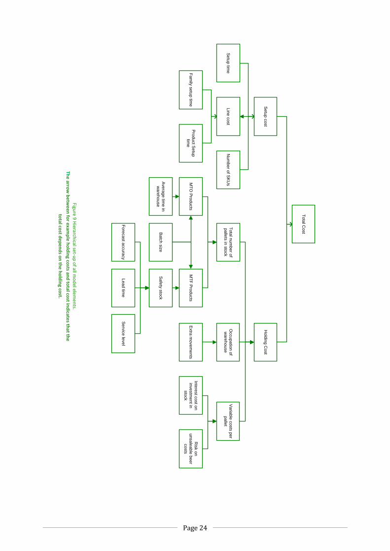
Figure 9 shows the structure of the elements in the model.
Page 24
To
tal C
ost
Se
tup
co
st
Ho
ldin
g C
ost
Lin
e c
ost
Se
tup
time
Nu
mb
er o
f SK
Us
Fa
mily
se
tup
time
Pro
du
ct S
etu
p
time
To
tal n
um
be
r of
pa
llets
in s
tock
Occu
pa
tion
of
wa
reh
ou
se
Va
riab
le c
osts
pe
r
pa
llet
MT
O P
rod
ucts
MT
F P
rod
ucts
Extra
mo
ve
me
nts
Inte
rest c
ost o
n
inve
stm
en
t in
sto
ck
Ris
k o
n
un
sa
lea
ble
be
er
co
sts
Ave
rag
e tim
e in
wa
reh
ou
se
Ba
tch
siz
eS
afe
ty s
tock
Fo
reca
st a
ccu
racy
Le
ad
time
Se
rvic
e le
ve
l
Figure 9
Hierarch
ical set-u
p o
f all mo
del elem
ents.
The
arrow
be
twe
en fo
r examp
le h
old
ing co
sts and
total co
st ind
icates th
at the
total co
st de
pen
ds o
n th
e h
old
ing co
st.

Page 25
5.1.1. Holding costs
As visualized in Figure 9, the holding cost that is an input for the total cost depends on several
factors: the average total number of pallets in the warehouse, the cost per pallet, and the level of
occupation of the warehouse.
The total number of pallets is a sum of both pallets with MTO and MTF product families. The
difference between pallets with MTO and MTF products is the duration of storage in the warehouse.
For MTO products the most important factor is the average duration (in weeks) in the warehouse,
which is assumed to be known.
For MTF products it is assumed that the stock level decreases linearly between the stock level
immediately after production, and the safety stock level. The stock level after production is the total
of the safety stock and the batch size, which can be determined using the total demand and the
number of setups. Figure 10 shows the assumed stock behaviour of an MTF product with a demand
of 250 pallets per week, batch size of 1000 pallets, safety stock of 1000 pallets, and production that is
not instantaneous.
Figure 10 Example for assumed stock behavior of MTF products
The favourable safety stock level is determined using the standard deviation of the forecast (for 1
week forward), a correction factor for the length of the production cycle, and a factor for the service
level. The correction factor ensures that the safety stock for a product that is produced every 4
weeks is larger than for a product that is produced every week, because uncertainty increases when
the time between production runs increases. The factor for the service level reflects the need for a
higher safety stock when a higher service level is agreed upon with the customers.
Within product families it is possible that several SKUs are produced on a MTO base and others on a
MTF base. In this case the total number of pallets of the family is a combination of the MTO and MTF
products. The percentage of total family volume is used to determine the weight of both types of
SKUs.
The variable costs are composed of the costs of working capital and the costs for the risk of
unsaleable beer. The cost of working capital is the interest the company on average pays on the
0
500
1000
1500
2000
2500
0
1
2
3
4
5
6
7
8
9
10
11
12
13
14
15
16
Sto
ck le
vel (
pal
lets
)
Weeks
MTF 4 weeks Average = Batch size/2 + Safety stock
Stock level

Page 26
value of the stock. The cost of the risk on unsaleable beer is the total of the costs of beer that is
removed because it has been too long in the warehouse or has been damaged by warehouse trucks.
The level of occupation is a factor in this model because extra forklift truck movements have to be
performed when occupancy of the warehouse is high, and external space has to be rented when
stock level becomes higher than the maximum warehouse capacity.
5.1.2. Setup costs
As Figure 9 shows, the setup costs depend on the costs of the line per hour, the time that is
necessary to perform a setup, and the number of SKUs in the family. The cost of the line per hour is
assumed to be known and constant. The time per setup has further been broken down into the time
to change to a new product family (new beer type) and the time it takes to do a small pack or label
change for products within the family. These times are also assumed to be known and constant.
It is further assumed that every family consists of one product with a high volume and a number of
products with a low volume. The one product with the high volume is produced every time that the
family is produced (the number of setups for this specific family as calculated by the calculation
model); the low volume products are filled the minimum number of setups as defined by the
constraints. For most products this is 12 times per year or once every month. The production of the
small products is then spread over the production runs. This results in the assumption that by
eliminating a setup, only the family setup time or cost is won.
5.1.3. Constraints
The model now determines the total setup and holding costs for any number of setups. However, in
reality the number of setups is restricted to some values. There are 3 factors that can restrict the
possible number of setups for products.
First, when a product has a lead time or shelf life of four weeks, it has to be produced at least every
four weeks, or 13 times per year. Second, products should not be produced more often than once
every week, to avoid inefficiency. Therefore the maximum number of setups per year is 52. Third, to
comply with set operating standards that state the minimum size of a production batch or MBS,
products can only be made as often as there are large enough batches.
5.1.4. Calculation model
The theoretical model is used to set up a cost calculation model that calculates the setup and holding costs per product family for different numbers of setups, brought together in the following total cost function:
Where for each product family , on production line , per
product family per line (pallets) is given, and for (# of setups) the following elements are
calculated:
: Setup cost per product or family of products (€)
: Total holding costs (€)
Appendix 2 states the formulations of the calculation model for and .

Page 27
5.1.5. Model setup and solver
To take product interactions, capacity constraints, and constraints such as maximum shelf time into
account, it is common to translate the complex problem to a deterministic model with linear
relations that can be solved in a linear program solver. Because we use a piece by piece linear
holding cost function, and want a solver that is easy to understand and operate, this model is built in
Excel and a solution with a certain tolerance to the optimum is found by using the Excel Solver
application.
To determine the quality of the output from the solver, the Excel solver function has a setting
“tolerance” that indicates the percentage that the objective value that is found may differ from the
true optimal value. By choosing for example 0,005 the program ensures to find a strategy that has a
total costs that is at most 0.5% higher than the total cost of the optimal strategy.
The solver function is further able to solve the problem with the condition that the number of setups
is an integer (whole number). Because the solver solves non-integer problems much faster than
integer problems, we do not use this function and assume that, for example half setups can be done.
5.2. Discussion of model
This section evaluates the proposed model by checking whether all characteristics of the actual
situation of Grolsch are implemented in the theoretical model.
Trade-off between setup and holding costs The trade-off between setup and holding costs is taken into account by the total cost function that is
a function of the setup and holding costs.
Product family dependent setup times, over time, and idle time In the model the setup times depend on the filling line the product is made on, as well as on the
family itself. It is however assumed that the setup costs per hour are known and constant, although
setups in overtime are more expensive and in idle time are less expensive.
Volatile demand Volatility of demand is not taken into account by the model because it uses an average demand as
input. By evaluating the suggested strategy per demand situation however, an analysis can be made
on how to perform in high or low demand situations.
Forecast Accuracy and Service Level The effect of forecast accuracy and service levels agreed in the SLAs is taken into account in the
safety stock calculations and thus incorporated in the holding costs.
MTO/MTF mix The distinction between MTO and MTF products is present in the model. The choice between MTO
and MTF has a result on the safety stock of the product (0 if MTO) and the average normal stock.
Maximum shelf life, lead time, and minimum batch size The constraints on maximum shelf life and lead time are both incorporated in the model by
restricting the possible values of the decision variable “number of setups”. The order acceptance
policy using a minimum batch size constrains the size of the batches and thus indirectly the number
of setups.

Page 28
Warehouse capacity The effects of the warehouse capacity have been dealt with by using a non-linear holding cost
function. Extra variable costs per pallet are used when extra warehouse space has to be temporarily
created and a bigger cost is set when the maximum capacity of the warehouse is met and pallets
should be stored outside.
Filling performance The influence of filling performance on Tactical Planning has not been taken into account. The model
suggests a strategy to optimize costs but does not take into account timing of setups. Thus it does
not give insight in how to schedule setups to reduce negative effects of unpredictable performance
of the filling lines.
Guaranteed global integer optimum The model is built in Excel and is optimized with the Excel Solver, which uses the branch and bound
method to determine the optimal value of the decision variables. The branch and bound method
calculates all possible combinations and thus ensures an optimal value within the margins set.
Accuracy From the above list we conclude that most of the characteristics of the Tactical Planning problem are taken into account in the model. There are however some limitations on for example the accuracy of the model:
As mentioned before, the model is allowed to advise 15.5 setups per year instead of only 15
or 16 for a product family. This can be prevented by using the integer constraint. However,
due to the uncertainty in reality, 15.5 setups can be a fine estimate for the rest of the year.
The line cost per hour is assumed to be known and constant, where in reality it depends on
the number of people manning the line and the type of employees (contract or temporary
labor).
For families with multiple SKUs it is assumed that one of the SKUs is produced every time the
family is produced and that all other SKUs are made the minimum number of times the
family should be produced as defined by the constraints. In reality, there commonly are
several SKUs that are filled every time a product family is filled.
For setups it is assumed that all products but one are made the minimum number of times.
For the stock level calculation, all products are made every time, resulting in a lower stock
level than actual and thus in less holding costs than actual. Increasing the number of setups
therefore results in more pallet savings than actual and is thus cheaper than in reality.
Reducing setups results in higher inventory costs and is thus more expensive than in reality.
It is assumed that the standard deviation of the RF is the same for 1 week in advance as for 4
weeks in advance. In reality, the forecast for a period of time further away in the future, is
more uncertain than a forecast for a period in the near future.
The SABMILLER assumption that a number of days for safety stock can be calculated only
from the standard deviation is not accurate. It should also reflect the demand pattern and
lead times of specific products. Furthermore, the model accepts that the safety can become
more than 5 days, while in practice Grolsch keeps 5 days and no more for all products.
5.3. Empirical research
This section defines the parameters of the cost calculation model for the specific situation of Grolsch.
To reduce complexity of the model and the number of calculations necessary, and thus computation

Page 29
times, we define parameters only for whole families of SKUs. Section 5.3.1 defines the input for the
calculation of holding costs, Section 5.3.2 defines setup costs, and Section 5.3.3 discusses the
accuracy of the assumptions made in the definitions.
5.3.1. Holding costs
Grolsch does not calculate an average holding cost per pallet for its warehouse; therefore we made
an estimation of the holding cost. For this calculation model only the variable costs are interesting
and they are non-linearly related to the number of pallets in the warehouse. When there are on
average more than 10.000 pallets in the warehouse, it is not possible to put every batch of beer in its
own warehouse position (which ranges between a position in a rack and a floor space of hundreds of
square meters). Therefore, forklift trucks have to combine small batches by making at most 150 extra
movements per week, with an estimated cost of 1 Euro per movement. This results in an increase of
the variable cost per pallet. When the stock level is between 12.500 and 16.000 pallets, again up to
150 extra movements are required to fit all products in the warehouse. The finished goods
warehouse has a net capacity of 16.300 pallets and when there are more pallets to be stored, some
space in the empty goods warehouse is cleared and used. Due to the relatively large distance to the
other warehouse and the assumption that the extra space is used as shortly as possible, this costs 2
extra movements per pallet per week, or 104 Euro per pallet per year. With a total capacity of 18.000
pallets in both warehouses, every extra pallet has to be stored at an external warehouse, estimated
to cost 10 Euro per pallet per week, or 520 Euro per pallet per year.
The described situation leads to the “cost of day to day stock level” function as seen in Figure 11. The
function is called “cost of day to day stock level” because the cost function assumes that the stock
level is precisely met every day of the year.
Because an average stock level of a year in reality includes weeks with much higher and much lower
actual stock, the function should be adjusted. For example, in a year with an average stock level of
13.000, there will be several weeks when stock needs to be moved to the empty goods warehouse
and thus the actual cost is higher than expected. We have studied two years of historical data and
found the “cost of yearly average stock level” function, as is shown in Figure 11.
p2; 12.500 p3; 16.300 p4; 18.000 p1; 10.000
Ho
ldin
g co
sts
(€)
Average stocklevel in pallets
Holding costs vs stocklevel
Cost of day to day stock level
Cost of yearly average stock level
Figure 11 Holding cost behaviour set out against stock level
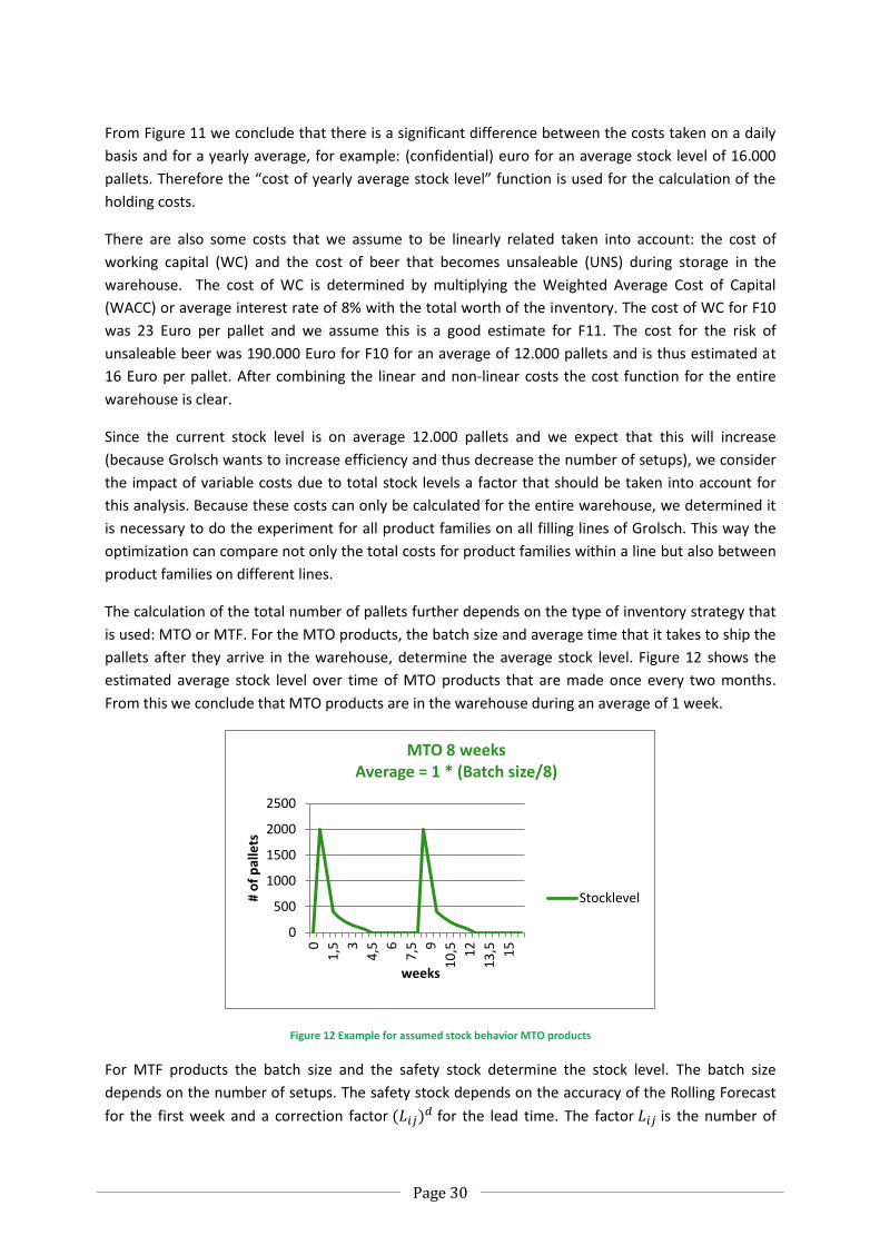
Page 30
From Figure 11 we conclude that there is a significant difference between the costs taken on a daily
basis and for a yearly average, for example: (confidential) euro for an average stock level of 16.000
pallets. Therefore the “cost of yearly average stock level” function is used for the calculation of the
holding costs.
There are also some costs that we assume to be linearly related taken into account: the cost of
working capital (WC) and the cost of beer that becomes unsaleable (UNS) during storage in the
warehouse. The cost of WC is determined by multiplying the Weighted Average Cost of Capital
(WACC) or average interest rate of 8% with the total worth of the inventory. The cost of WC for F10
was 23 Euro per pallet and we assume this is a good estimate for F11. The cost for the risk of
unsaleable beer was 190.000 Euro for F10 for an average of 12.000 pallets and is thus estimated at
16 Euro per pallet. After combining the linear and non-linear costs the cost function for the entire
warehouse is clear.
Since the current stock level is on average 12.000 pallets and we expect that this will increase
(because Grolsch wants to increase efficiency and thus decrease the number of setups), we consider
the impact of variable costs due to total stock levels a factor that should be taken into account for
this analysis. Because these costs can only be calculated for the entire warehouse, we determined it
is necessary to do the experiment for all product families on all filling lines of Grolsch. This way the
optimization can compare not only the total costs for product families within a line but also between
product families on different lines.
The calculation of the total number of pallets further depends on the type of inventory strategy that
is used: MTO or MTF. For the MTO products, the batch size and average time that it takes to ship the
pallets after they arrive in the warehouse, determine the average stock level. Figure 12 shows the
estimated average stock level over time of MTO products that are made once every two months.
From this we conclude that MTO products are in the warehouse during an average of 1 week.
Figure 12 Example for assumed stock behavior MTO products
For MTF products the batch size and the safety stock determine the stock level. The batch size
depends on the number of setups. The safety stock depends on the accuracy of the Rolling Forecast
for the first week and a correction factor for the lead time. The factor is the number of
0
500
1000
1500
2000
2500
0
1,5
3
4,5
6
7,5
9
10
,5
12
13
,5
15
# o
f p
alle
ts
weeks
MTO 8 weeks Average = 1 * (Batch size/8)
Stocklevel

Page 31
weeks lead time and can be estimated empirically. We assume that the standard deviation in time
is always the same and thus use . Furthermore we assume that for every 20% of corrected
standard deviation a set number of days of safety stock has to be held, determined by the service
level.
Service level (%) 90% 95% 99%
St. Deviation of 1 week RF (%) 20% 20% 20%
Safety stock (days) (confidential) Table 2 Example values for s from the Grolsch case.
The current calculation uses a service level of 99% for all products because this is standard for SLAs,
and a standard deviation of 40% because Grolsch works with a policy of 5 days of safety stock for all
its products. Therefore, in the current model safety stock is mostly between 5 days for weekly
produced products and 9 days for monthly products and additionally only depends on the demand
per year. When the stock levels of all MTO and MTF products are added to the total stock level, and
the holding cost function is known, we can calculate the total cost of holding stock.
5.3.2. Setup costs
For the setup times we used the operating standards as used by the operational planners in July 2011
and line costs provided by the Supply Chain Controller. Setup times are derived from the operating
agreements, set per product family, and divided in three types: family setups/brand changes, pack
changes, and label changes.
5.3.3. Discussion
Since the costs were not exactly known and for example the relation between number of setups and
the number of times products are actually produced is not clear, the following inaccuracies are
identified:
1. The holding cost function is based on a five year old assumption on the number of extra
movements required and costs per movement.
2. The MTO stock level is based on an estimated average period in the warehouse for MTO
products of 1 week. No historic analysis was done to underpin this estimation.
3. For MTF products, the safety stock level is between 5 and 9 days dependent on number of
setups, and further only depends on the demand per year. Using accurate standard
deviations per product family would make the model a lot more accurate and could identify
room for improvement that is not visible at the moment.
4. Working capital costs and unsaleable beer costs per pallet per year are assumed to be equal
for all types of beer on any type of pallet (which have volumes between 5.5 and 9 hectolitre).
5. The setup times are averaged and based on operating standards, not on actual performance.
6. The cost per line assumes that for every hour that is saved, a constant amount of money is
saved. In reality, depreciation costs stay equal when the number of factory hours decreases,
and personnel costs are only reduced when employees are actually fired.
7. The demand used for the analysis is the RF for F12, the next year. Because the RF is very
uncertain, every strategy that comes from the model should be reviewed on a monthly basis.
8. The line costs per hour do not change when demand and thus occupation increases. In
practice, overtime may be required when there is too much production per week.
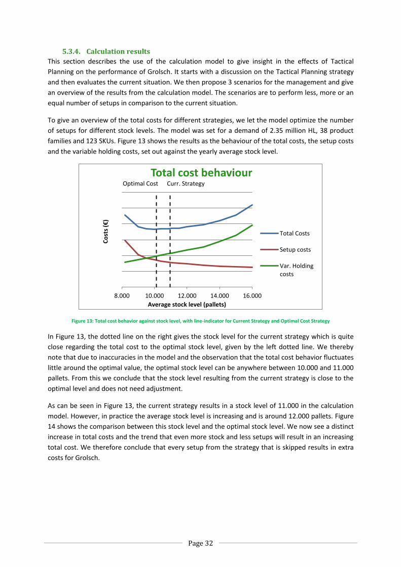
Page 32
5.3.4. Calculation results
This section describes the use of the calculation model to give insight in the effects of Tactical
Planning on the performance of Grolsch. It starts with a discussion on the Tactical Planning strategy
and then evaluates the current situation. We then propose 3 scenarios for the management and give
an overview of the results from the calculation model. The scenarios are to perform less, more or an
equal number of setups in comparison to the current situation.
To give an overview of the total costs for different strategies, we let the model optimize the number
of setups for different stock levels. The model was set for a demand of 2.35 million HL, 38 product
families and 123 SKUs. Figure 13 shows the results as the behaviour of the total costs, the setup costs
and the variable holding costs, set out against the yearly average stock level.
Figure 13: Total cost behavior against stock level, with line-indicator for Current Strategy and Optimal Cost Strategy
In Figure 13, the dotted line on the right gives the stock level for the current strategy which is quite
close regarding the total cost to the optimal stock level, given by the left dotted line. We thereby
note that due to inaccuracies in the model and the observation that the total cost behavior fluctuates
little around the optimal value, the optimal stock level can be anywhere between 10.000 and 11.000
pallets. From this we conclude that the stock level resulting from the current strategy is close to the
optimal level and does not need adjustment.
As can be seen in Figure 13, the current strategy results in a stock level of 11.000 in the calculation
model. However, in practice the average stock level is increasing and is around 12.000 pallets. Figure
14 shows the comparison between this stock level and the optimal stock level. We now see a distinct
increase in total costs and the trend that even more stock and less setups will result in an increasing
total cost. We therefore conclude that every setup from the strategy that is skipped results in extra
costs for Grolsch.
Curr. Strategy Optimal Cost
8.000 10.000 12.000 14.000 16.000
Co
sts
(€)
Average stock level (pallets)
Total cost behaviour
Total Costs
Setup costs
Var. Holding costs

Page 33
Figure 14: Total cost behavior against stock level, with line-indicator for Current stock level and Optimal Cost Strategy
When we assume that in the situation of the optimal cost level, an investment of 60.000 Euro is
allowed to increase company performance on KPIs, the stock level may vary between 9.000 and
13.000 pallets. In Figure 15, the total cost is put out against Working Capital and the gap in Factory
Efficiency. Because the performance of the filling department is measured in Factory Efficiency that
increases when the number of setups is reduced, the optimal stock level for the FE ratio is the
maximum stock level of 13.000 pallets. However, the investments made in the value of the stock
increase when the stock level increases, thus the minimum stock level of 9.000 pallets is the optimal
level for the costs of and investment in stock.
Figure 15: Total costs (€) vs. the efficiency gap by setups (in %) and Working Capital (€)
Current. Stock Optimal Cost
8.000 10.000 12.000 14.000 16.000
Co
sts
(€)
Average stock level (pallets)
Total cost behaviour
Total Costs
Setup costs
Var. Holding costs
Current stock Improve FE improve WC
0,0%
2,0%
4,0%
6,0%
8,0%
10,0%
12,0%
0
200.000
400.000
600.000
800.000
1.000.000
1.200.000
8.000 10.000 12.000 14.000 16.000
Fact
ory
Eff
icie
ncy
gap
(%
)
Co
sts
(€)
Average stock level (pallets)
Total costs vs. WC costs and Efficiency gap
Total Costs
Working Capital Costs
Efficiency Gap (%)
Co
nfi
den
tial

Page 34
Production Efficiency or cost savings? Within the area between 9.000 and 13.000 pallets of stock, Grolsch can choose to reduce
investments in stock by increasing the number of setups, have the lowest possible cost by keeping to
the optimal strategy, or to improve Factory Efficiency by decreasing setups. To evaluate the benefits
of all stated average stock levels, we now set the model to optimize the number of setups, to
minimize the total costs, for the stated stock levels: “optimal for Working Capital” (9.000 pallets),
“optimal for Cost” (11.000 pallets), “current stock level” (12.000 pallets) and “optimal for Factory
Efficiency” (13.000 pallets).
Improve WC Optimal Cost Current Stock Improve FE
Average stock level (# of pallets) 9.000 10.000 12.000 13.000
Working Capital costs (confidential) Total holding costs
Investment in Working Capital
# of setups per year 782 625 472 425
Setup time (hours) (confidential) Efficiency gap
Total setup costs
Total costs (confidential) Table 3 Model results for total bottling
From Table 3 we conclude that implementing the optimal strategy would save 30.000 Euro, free up
575.000 Euro from the decreased stock, and increase the efficiency gap by 0,8% of FE. Saving 0,2% FE
would however cost Grolsch 30.000 Euro. However, when Grolsch stops using the FE as a KPI and
would optimize for Working Capital, 870.000 Euro in stock investments could be reduced, without
costs but with an increase of 329 setups and thus an increase of the efficiency gap by 1,6% FE.
However, the above conclusion does not mean that for every (confidential) Euro 0,2% FE is saved.
From Figure 16, an example of line 8, we conclude that the lowest possible cost of Efficiency through
setups for line 8 is around 4,8% at an additional cost of (confidential) Euro.
Figure 16: Total costs of the filling department and only for line 8 set out against the Efficiency Gap by setups (%) for line 8.
Curr. Strategy Current. Stock Improve Cost
0,0%
1,0%
2,0%
3,0%
4,0%
5,0%
6,0%
7,0%
8,0%
0
200.000
400.000
600.000
800.000
1.000.000
1.200.000
8.000 10.000 12.000 14.000 16.000
Effi
cie
ncy
Gap
(%
)
Co
sts
(€)
Average stock level (pallets)
Line 8 Total Costs vs. Efficiency Gap
Total costs
Total costs line 8
Efficiency Gap (%)
Co
nfi
den
tial
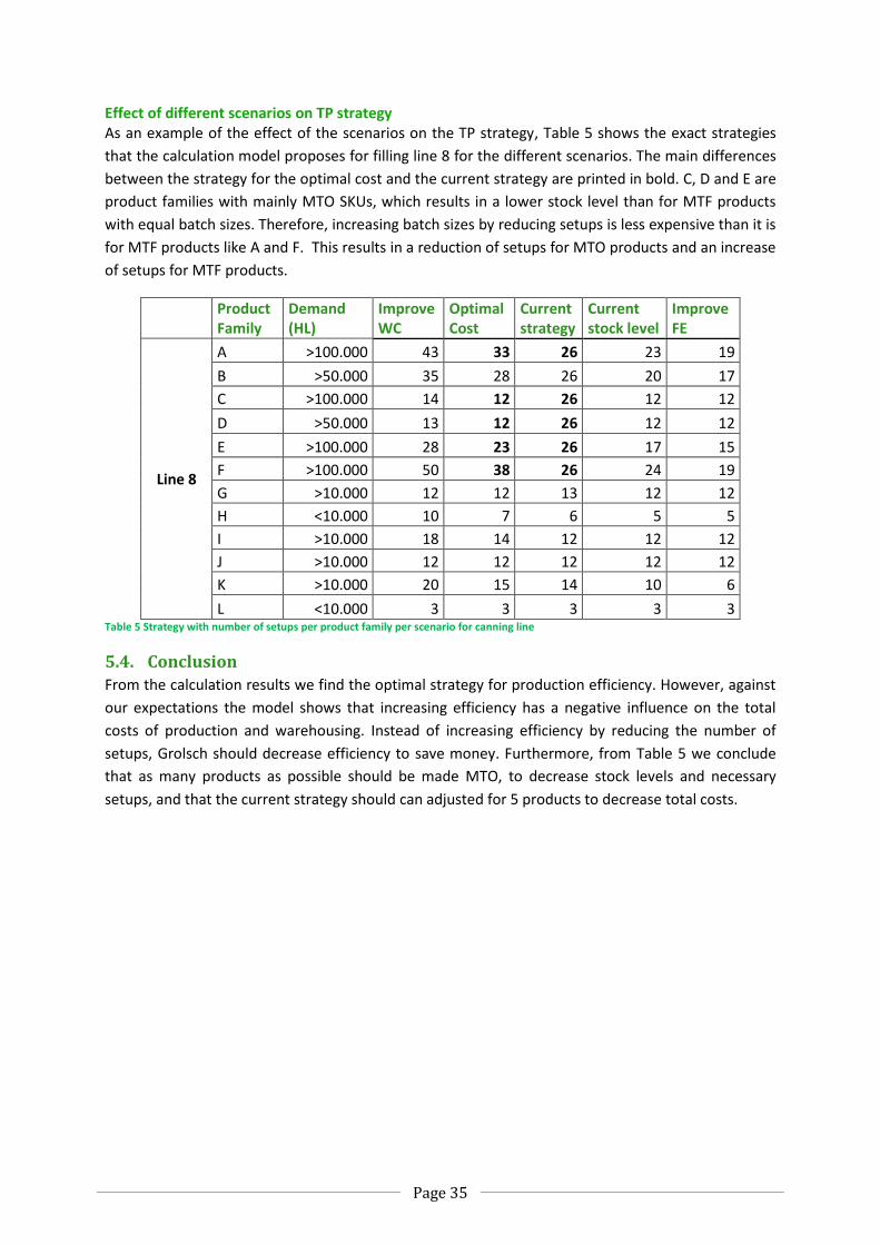
Page 35
Effect of different scenarios on TP strategy As an example of the effect of the scenarios on the TP strategy, Table 5 shows the exact strategies
that the calculation model proposes for filling line 8 for the different scenarios. The main differences
between the strategy for the optimal cost and the current strategy are printed in bold. C, D and E are
product families with mainly MTO SKUs, which results in a lower stock level than for MTF products
with equal batch sizes. Therefore, increasing batch sizes by reducing setups is less expensive than it is
for MTF products like A and F. This results in a reduction of setups for MTO products and an increase
of setups for MTF products.
Product Family
Demand (HL)
Improve WC
Optimal Cost
Current strategy
Current stock level
Improve FE
Line 8
A >100.000 43 33 26 23 19
B >50.000 35 28 26 20 17
C >100.000 14 12 26 12 12
D >50.000 13 12 26 12 12
E >100.000 28 23 26 17 15
F >100.000 50 38 26 24 19
G >10.000 12 12 13 12 12
H <10.000 10 7 6 5 5
I >10.000 18 14 12 12 12
J >10.000 12 12 12 12 12
K >10.000 20 15 14 10 6
L <10.000 3 3 3 3 3 Table 5 Strategy with number of setups per product family per scenario for canning line
5.4. Conclusion
From the calculation results we find the optimal strategy for production efficiency. However, against
our expectations the model shows that increasing efficiency has a negative influence on the total
costs of production and warehousing. Instead of increasing efficiency by reducing the number of
setups, Grolsch should decrease efficiency to save money. Furthermore, from Table 5 we conclude
that as many products as possible should be made MTO, to decrease stock levels and necessary
setups, and that the current strategy should can adjusted for 5 products to decrease total costs.

Page 36
6. Conclusion and discussion This chapter states the conclusions of this research in Section 6.1. Section 6.2 discusses the
limitations of the research and Section 6.3 the recommendations for further research and
implementation of the model.
6.1. Conclusion
The trigger for this research is the Tactical Planning strategy that needs improvement for production
efficiency of the filling lines by taking costs, warehouse capacity, SLAs and uncertainties into account.
The described problem leads to the following problem statement:
Which factors influence the medium-term planning
and how can Grolsch optimize the tactical planning strategy for the efficiency of production?
This research identifies 20 factors that influence the Tactical Planning and thus the planned
efficiency. After evaluating all influencing factors, we conclude that the forecast inaccuracy, demand
volatility, and deviations from planning by filling lines are the main negative factors on the planned
efficiency. Furthermore the planners expect that the maximum age of beer and warehouse capacity
will gain more influence when batch sizes are increased. We finally conclude that Tactical Planning
can only influence the planned efficiency by its Tactical Planning strategy.
To optimize the planning strategy for production efficiency we propose a model in Chapter 4, which
we use in Chapter 5 to calculate the optimal strategy and the costs of several scenarios. From this
analysis we conclude that the current Tactical Planning strategy is close to or at its optimum
regarding the stock level, but has to be adjusted for specific product families as stated in Appendix 3.
Although the current strategy stock level is near the optimal stock level, the actual stock level is too
high, due to deviations from the strategy.
The total efficiency of the filling department can be improved by 0.2% in comparison with the current
strategy by increasing the total costs by an estimate of 30.000 Euro. Because the effect of increasing
production efficiency by decreasing the number of setups is an increase of total costs, we conclude
that the Tactical Planning should not optimize its planning for production efficiency, but instead
optimize its planning to minimize total costs or minimize the investments in stock.
So we recommend Grolsch to focus more on the interaction between departments. It is important
for TP to refine the variable warehousing costs per pallet and take the costs into consideration in its
decision making processes. In the decision to make a product MTO or MTF, we advise to make as
many products on an MTO basis as possible to reduce stock levels and thus holding costs.
Regarding the TP, the current strategy has proven to be near to the optimal strategy. However,
because TP assumes that production efficiency improves the total cost, TP is currently deviating from
the current strategy. Because these deviations have a negative impact on total costs, we strongly
advise to follow the TP strategy more strictly.
The calculation model we present in this research works well to illustrate this and almost instantly
provides strategies for the optimization of any arbitrary scenario. We calculate the results of two
scenarios under the assumption of equal forecast accuracy for all products and the estimated
forecasted demand of F12.

Page 37
When we optimize for lowest total cost we estimate that 30.000 Euro per year can be saved and
570.000 Euro of investments in stock can be released. When we optimize for stock investments we
estimate that 870.000 Euro of investments in stock can be redirected without a higher total cost level
than Grolsch currently has.
6.2. Limitations and recommendations
The research has some limitations that we discuss in this section. Section 6.2.1 discusses the
limitations of the overall research and Section 6.2.2 discusses the limitations of the calculation
model.
6.2.1. Limitations of the research
The research is done on the effect of Tactical Planning on the efficiency of the filling lines. We find
that the Tactical Planning has an influence on the efficiency through the planned number of setups
and the robustness of the planning. However, the research was limited to the calculation of the
number of setups, and the influence of robustness is not taken into account in the calculation model.
Furthermore, the effect on production efficiency was only determined for the Tactical Planning
strategy, not for other Tactical Planning steps like the MTO/MTF decision. Moreover, the calculation
model takes only the trade-off between holding costs and setup costs into account and does not
include the effect on the brewing and commercial departments.
Last, the output of the model is only compared with the current strategy and current stock level. The
performance of the optimization cannot be determined by these comparisons.
6.2.2. Limitations of the calculation model
The calculation model does not take all factors that have an influence on the Tactical Planning into
account. The limitations we think are important for the performance of the model are:
The calculation model does not take volatile demand into account. The volatility of demand
is one of the main problems for TP and creates the biggest risks for Grolsch.
The model is based on product families. Therefore, the optimal behaviour of specific
products cannot be determined by the calculation model. The current model is only
corrected by the possibility to determine the volume of MTF and MTO within product
families
The setup costs do not take into account the occupancy of the filling lines. When demand is
more than can be produced in normal factory hours, overtime has to be made, which is more
expensive. Eventually, when the demand for a filling line exceeds the maximum capacity,
extra hours of downtime would cost the margin on all missed production and would become
very high
The calculation model does not take timing into account. The number of setups per month is
determined but it is not clear in which weeks the setups should be scheduled. The scheduling
effect is also not taken into account in the calculation of the strategy
6.3. Recommendations
During the research, choices and assumptions were made that restricted the research to less than all
possible options. Because we found some interesting subjects that were outside the scope of this
research, we now recommend on the use of the current calculation model and on future research.

Page 38
6.3.1. Possible uses of the current calculation model
The model can be used to evaluate more aspects of the Tactical Planning than it has been used for in
this research:
By loosening the lead-time constraint the effect of the current SLAs on the total cost
becomes visible. The effect can then be evaluated to decide whether SLAs need
renegotiation
Through converting the yearly calculation model to a monthly model it can be used to create
strategies for different months during a year. By changing demand, the optimal behaviour for
high and low demand seasons can be determined
Different safety stock strategies can be entered and evaluated for e.g. total costs, working
capital costs, and effect on efficiency.
6.3.2. Future research
During this research we observed several subjects that are interesting for future research at Grolsch.
We therefore recommend Grolsch to:
Refine the setup and holding costs as found in this research to include all important costs in
cooperation with the production and warehousing departments to ensure organization
support and acknowledgment of modelling results.
Investigate the costs and benefits of the implementation of the TP strategy in the currently
used ERP software. Implementing the strategy can save a lot of handwork and make room
for more focus on performance and robustness of the planning.
Investigate the timing of the setups/batches, with the goal to increase stability in the
brewery and filling department.
Investigate the possibility to taking the brewing and filtration into account for Tactical
Planning. By setting up a model that calculates the effect on all departments, proposed
improvements can be valued more accurately.
Analyse the safety stock strategy. The use of 5 days of safety stock for fast moving products
as well as for slow moving products is not as optimal as determining a safety stock strategy
for different product or product families.
Investigate the effect of planned downtime on unplanned downtime. Within Grolsch, the
assumption is made that less setups lead to a more stable production performance.
However, even the lines with practically no setups still have considerable downtimes due to
breakdowns. We think it could be possible that more setups lead to a better and continuous
insight in the state of the line and will reduce the time lost by breakdowns.
Compare the outcomes of this research with the outcomes of the ELSP Heuristic as proposed
in the literature review.

Page 39
7. References Drexl, A. and A. Kimms (1997). "Lot sizing and scheduling - Survey and extensions." European Journal
of Operational Research 99(2): 221-235. Harris, F. W. (1913). "How Many Parts to Make at Once" Factory: The Magazine of Management
10(2): 135-136, 152. Hopp, W. J. and M. L. Spearman (2008). Factory physics. New York, NY, McGraw-Hill/Irwin/Irwin. Hsu, W. L. (1983). "On the General Feasibility Test of Scheduling Lot Sizes for Several Products on One
Machine." Management Science 29(1): 93-105. Tarim, S. A. and B.G. Kingsman (2004). "The stochastic dynamic production/inventory lot-sizing
problem with service-level constraints." International Journal of Production Economics 88(1): 105-119.
Soman, C. A., D.P. van Donk and G. Gaalman (2004). "Combined make-to-order and make-to-stock in a food production system." International Journal of Production Economics 90(2): 223-235.
Taft, E. W. (1918). "Formulas for exact and Approximate Evaluation - Handling Cost of Jigs and Interest Charges for Product Manufactured Included" The Iron Age 101: 1410-1412.
Visser, H. M. and v. A. R. Goor (2007). Op weg naar Supply Chain Management, Noordhoff Uitgevers.

Page 40
8. Appendices
Appendix 1: Model formulation
For each product family on production line the following parameters are
given:
: Demand (HL)
: Demand (pallets)
: Number of SKUs (# per product family)
: Family setup cost (€ per setup)
: Product setup cost (€ per setup)
: Minimum number of setups
: Maximum number of setups
: Standard deviation for 1 week RF (number)
CV : Covariant of Variation (percentage) : Percentage of product family volume for MTF products : Number of weeks an MTO product is on average in the warehouse. : Maximum lead time (weeks)
: Maximum shelf life (weeks)
: Minimum Batch size (HL)
: Volume per pallet (HL)
Furthermore, for the specific warehouse the following parameters are given: : Costs of lower levels (€) : Variable costs for the pallet level (€) : Fixed costs per pallet (€) : Cost of working capital per pallet (€) : Cost of unsaleable beer risk per pallet (€) the model than sets: : The number of setups
and calculates: : Batch size (pallets)
: Total setup cost per family (€ per setup)
: Total holding costs (€) : Total average number of pallets : Average number of pallets for product on line in warehouse
: Average number of pallets for product on line if it is an MTO product.
: Average number of pallets for product on line if it is an MTF product.
: Safety stock (# of pallets)
: Correction on standard deviation for production time
: Constant estimated empirically
To find the total cost value that is minimized using the objective function.
Objective function

Page 41
The objective is to minimize the total costs. This formula minimizes the sum of the setup and holding
costs through the following calculation: Minimize ((setup costs * number of setups) + total holding
costs)
Demand Because demand is given in HL, we first have to transform it to number of pallets by dividing it by the
volume per pallet.
Batch size The average batch size depends on the total production quantity of a year and the number of times
the product is produced.
Setup costs
The setup costs of a product family depends on the line it is made on and the number of SKUs that is
in the family. We assume that if a product should minimally be made 5 times per year but is made 10
times per year, 10 big family setups are required , and for all other SKUs
(number of SKUs minus 1 for the family setup) 5 small setups. Only one product is thus made every
time and the other products are made the minimum number of times.
Holding costs The holding costs depend on the stock level and the function is not overall linear. Between 6
boundaries (0, p1, p2, p3, p4, ∞) however there are linear relations assumed. There is a base cost
for every pallet and it is increased with an increasing variable cost per pallet . To keep track
of the costs inflicted between lower boundaries, a variable is included that is the sum of all
lower level variable costs.
The cost for holding stock now depends the average stock level P and the values for a, b and C. For
clarity, some example values are given in the following table for every stock level P.
P Base Var Lower
P < p1 38.85 0 0 p1 < P < p2 38.85 3.12 0 p2 < P < p3 38.85 2.05 7.800 (3.12*(p2-p1) p3 < P < p4 38.85 104 15.600 (7800 + 2,05*(p3-p2)
p4 < P 38.85 520 192.400 (1560 + 104*(p4-p3) Table 4 Exemplary values for a, b and c for different stock levels from the Grolsch case.
The base cost value for every pallet depends on two costs: costs for working capital and
cost for unsaleable products .

Page 42
The average stock level of the warehouse is the sum of the average stock levels of all product
families.
The average stock level per product family depends on the composition of MTO and MTF products.
When the family consists only of MTF products, MTFO is 1. When the family consists only of MTO
products, MTFO is 0. When the product family is evenly composed of MTO and MTF products, for
half of the products the MTF stock level is calculated and for the other half the MTO calculation is
used.
For MTO products, the number of weeks the products on average stay in the warehouse is given by
parameter . The average stock level is then the number of products that is made per
batch, divided by the number of weeks between production runs, multiplied by .
For MTF products it is assumed that safety stock is always present and the stock level fluctuates
linearly between the safety stock level and the ‘safety stock + batch size’ level.
Safety stock is calculated with a combined formula from SABMILLER and scientific literature. The
standard deviation of the RF for 1 week forward in percentage is adjusted for the actual time
between production batches by . L is the number of weeks between production and d is a
constant that is assumed to be 0.5. Then following the SABMILLER procedures, for every 20% of
standard deviation, a number of days of safety stock ( ) is used to find the total days of safety stock
that is required. The number of pallets is then used by multiplying the number of days with the
demand per day.
For example, in the Grolsch case for every 20% standard deviation of a product with an agreed
service level of 99%, 2.3 days of safety stock ( ) are held.
Constraints If the lead time for a product is 4 weeks, production should incur as frequent as or more frequently
than every 4 weeks to insure that agreements are met. The same holds for shelf life of a product.
To comply with set operating standards that state the minimum size of a production batch or MBS,
the following constraint is used.

Page 43
Appendix 2: Tactical Planning Strategy Scenarios
Setups /year Product
Family
Working Capital Total cost
Current strategy
Current performance
Factory Efficiency
9.000 pallets 10.000 pallets 11.000 pallets 12.000 pallets 13.000 pallets
Line 1
F 52 49 52 30 24
E 34 26 26 18 16
G 18 14 26 12 12
M 9 8 6 6 6
R 2 2 2 2 2
P 15 13 13 13 14
L 10 10 10 10 10
Line 2
R 16 11 12 8 7
M 25 19 18 14 12
Q 19 14 14 11 9
P 13 9 7 7 9
L 16 12 10 9 8
Line 3 F 52 52 52 52 52
E 13 12 12 12 12
Line 4 F 45 33 26 24 21
E 52 52 26 34 26
Line 5
F 2 2 2 2 2
E 4 4 4 4 4
M 1 1 1 1 1
Line 7
F 20 13 13 10 8
E 36 27 27 20 18
N 9 5 5 4 4
C 32 23 26 17 16
D 20 13 26 12 12
G 48 35 26 25 21
O 14 9 13 7 6
Line 8
A 43 33 26 23 19
B 35 28 26 20 17
C 14 12 26 12 12
D 13 12 26 12 12
E 28 23 26 17 15
F 50 38 26 24 19
G 12 12 13 12 12
H 10 7 6 5 5
I 18 14 12 12 12
J 12 12 12 12 12
K 20 15 14 10 6
L 3 3 3 3 3
Table 5 Modeling results for current strategy, current performance and 3 scenarios