Ba7202 financial management (unit2) notes

Financial Management Semester II

S.N.Selvaraj, Assistant Professor, E-mail: [email protected]

UNIT – II: INVESTMENT DECISIONS

Capital Budgeting: Principles and Techniques – Nature of Capital Budgeting –

Identifying Relevant Cash Flows – Evaluation Techniques: Payback – Accounting

Rate of Return – Net Present Value – Internal Rate of Return – Profitability Index –

Comparison of DCF Techniques – Project Selection under Capital Rationing –

Inflation and Capital Budgeting – Concept and Measurement of Cost of Capital –

Specific Cost and Overall Cost of Capital

CAPITAL BUDGETING: PRINCIPLES AND TECHNIQUES

An efficient allocation of capital is the most important finance function in the modern

times. It involves decisions to commit the firm‟s funds to the long-term assets.

Capital budgeting or investment decisions are of considerable importance to the firm,

since they tend to determine its value by influencing its growth profitability and risk.

The long-term assets are those that affect the firm‟s operations beyond the one-year

period. The firm‟s investment decisions would generally include expansion,

modernization and replacement of the long-term assets. Sale of a division or business

(divestment) is also as an investment decision.

According to Charles T Horngren, “The Capital budgeting is a long-term planning for

making and financing the proposed capital outlays”.

According to R.M.Lynch, “Capital budgeting consists in planning, the development of

available capital for the purpose of maximizing the long term profitability (return on

investment) of the firm”.

The following are the features of capital budgeting:

The exchange of current funds for future benefits

The funds are invested in long-term assets

The future benefits will occur to the firm over a series of years

The long-term effect influence the decision and cannot be changed so easily

There exist a great deal of risk and uncertainty

Principles of Capital Budgeting

1) Decisions are based on cash flow not accounting income.

2) Timing of cash flows

3) Opportunity cost should be considered

4) Cash flows should adjusted for taxes

5) Financing cost should be ignored

There are several techniques available for evaluation of capital budgeting and can be

classified into two broad categories such as Non-discounted Cash Flow Methods and

Discounted Cash Flow Methods.



NATURE OF CAPITAL BUDGETING

The nature of capital budgeting includes the decisions involve the exchange of current

funds for the benefits to be achieved in future. Capital budgeting requires special

attention because of the following reasons:

They influence the firm‟s growth in the long run

They affect the risk of the firm

They involve commitment of large amount of funds

They are among the most difficult decisions to make

The future benefits are expected to be realized over a series of years.

The funds are invested in non-flexible and long term activities.

Types of Investment Decisions/Capital Budgeting

There are many ways to classify investments. They are as follows:

Expansion and Diversification

Replacement and Modernization

Mutually Exclusive Investments

Independent Investments

Contingent Investments

Expansion and Diversification: A company may add capacity to its existing product

lines to expand existing operations. For example, the Gujarat State Fertilizer Company

(GSFC) may increase its plant capacity to manufacture more urea. It is an example of

related diversification.

A firm may expand its activities in a new business. Expansion of new business

requires investment in new products and a new kind of production activity within the

firm. If a packaging manufacturing company invests in a new plant and machinery to

produce ball bearing, which the firm has not manufactured before, this represents

expansion of new business or unrelated diversification.

Sometimes a company acquires existing firms to expand its business. In either case

the firm makes investment in the expectation of additional revenue. Investments in

existing or new products may also be called as revenue-expansion investments.

Replacement and Modernization: The main objective of modernization and

replacement is to improve operating efficiency and reduce costs. Cost savings will

reflect in the increased profits, but the firm‟s revenue may remain unchanged. Assets

become outdated and obsolete with technological changes. The firm must decide to

replace those assets with new assets that operate more economically.

Mutually Exclusive Investments: Mutually exclusive investments serve the same

purpose and compete with each other. If one investment is undertaken, others will

have to be excluded. A company may, for example, either use a more labour-

intensive, semi-automatic machine, or employ a more capital-intensive, highly

automatic machine for production.



Independent Investments: Independent investments serve different purposes and do

not complete with each other. For example, a heavy engineering company may be

considering expansion of its plant capacity to manufacture additional excavators and

addition of new production facilities to manufacture a new product – light commercial

vehicles.

Contingent Investments: Contingent investments are dependent projects; the choice of

one investment necessitates undertaking one or more other investments. For example,

if a company decides to build a factory in a remote, backward area, it may have to

invest in houses, roads, hospitals schools, etc., for the employees to attract the work

force.

IDENTIFYING RELEVANT CASH FLOWS

One of the most important capital budgeting tasks for the evaluation of the project

capital investments is the estimation of the relevant cash flows for each project.

Estimating cash flows is critical because inaccurate or unreliable data can corrupt the

entire capital budgeting process. Estimating a new project‟s cash flows involves great

uncertainty and may be little more than educated guesswork.

Elements of Cash Flows

To evaluate a project, one must determine the relevant cash flows, which are the

incremental after-tax cash flows associated with the project.

a) Initial Investment:The initial investment is the after-tax outlay on capital

expenditure and net working capital is set-up.

b) Operating Cash Inflows:The operating cash flows are the after-tax inflows

resulting from the operations of the project during its economic life.

c) Terminal Cash Inflows:The terminal cash inflow is the after-tax cash flow

resulting from the liquidation of the project at the end of its economic life.

Capital Budgeting Process

The following procedure may be adopted in the process of capital budgeting:

Identification of Investment Proposals

Screening the Proposals

Evaluation of Various Proposals

Fixing Priorities

Final Approval and Preparation of Capital Expenditure Budget

Implementing Proposal

Performance Review

EVALUATION TECHNIQUES

A number of investment criteria or capital budgeting techniques are use in practice.

They may be grouped in the following two categories.



Discounted Cash Flow (DCF) Criteria

o Net present value (NPV)

o Internal rate of return (IRR)

o Profitability index (PI)

Non-discounted Cash Flow Criteria

o Payback (PB)

o Accounting rate of return (ARR)

PAYBACK METHOD

Pay back is one of the oldest and commonly used methods for explicitly recognizing

risk associated with an investment project. This method, as applied in practice, is

more an attempt to allow for risk in capital budgeting decision rather than a method to

measure profitability. Business firms using this method usually prefer short payback

to longer ones and often establish guidelines that a firm should accept investments

with some maximum payback period, say three or five years.

For example, two projects with, say, a four-year payback period are at very different

risks if in one case the capital is recovered evenly over the four years, while in the

other it is recovered in the last year. Obviously, the second project is more risky. If

both cease after three years, the first project would have recovered three-fourths of its

capital, while all capital would be lost in the case of second project.

Thus, the payback (PB) is one of the most popular and widely recognized traditional

methods of evaluating investment proposals. Pay back is the number of years required

to recover the original cash outlay invested in a project. If the project generates

constant annual cash inflows, the payback period can be computed by dividing cash

outlay by the annual cash inflow. That is,

Pack back = Initial Investment = C0

Annual Cash Inflow C

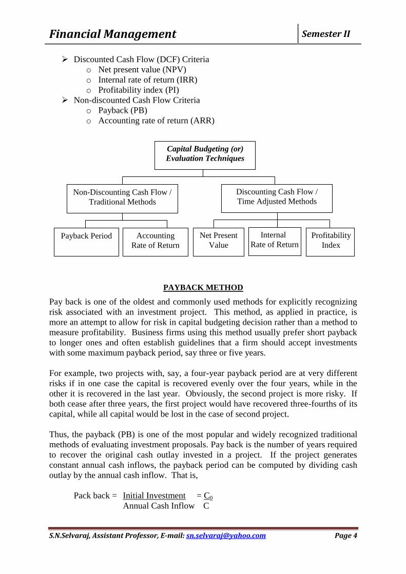
Capital Budgeting (or)

Evaluation Techniques

Non-Discounting Cash Flow /

Traditional Methods

Discounting Cash Flow /

Time Adjusted Methods

Payback Period Accounting

Rate of Return

Net Present

Value

Internal

Rate of Return Profitability

Index



Problem: Payback (Constant Cash Flow)

Suppose that a project requires a cash outlay of Rs.20,000 and generate cash inflows

of Rs.8000, Rs.7000, Rs.4000 and Rs.3000 during the next 4 years. What is the

project‟s payback?

Solution:When we add up the cash inflows, we find that in the first three years

Rs.19000 of the original outlay is recovered. In the fourth year cash inflow generated

is Rs.3000 and only Rs.1000 of the original outlay remains to be recovered.

Assuming that the cash inflows occur evenly during the year, the time required to

recover Rs.1000 will be (Rs.1000/Rs.3000)*12 months = 4 months. Thus, the

payback period is 3 years and 4 months.

Evaluation of Payback

Payback is a popular investment criterion in practice. It is considered to have certain

virtues.

Simplicity:The most significant merit of payback is that it is simply to

understand and easy to calculate. The business executives consider the

simplicity of method as a virtue.

Cost effective:Payback method costs less than most of the sophisticated

techniques that require a lot of the analysis‟ time and the use of computers.

Short-term effects: A company can have more favourable short-run effects on

earnings per share by setting up a shorter standard payback period.

Risk shield:Therisk of the project can be tackled by having a shorter standard

payback period as it may ensure guarantee against loss. A company has to

invest in many projects where the cash inflows and life expectancies are highly

uncertain.

Liquidity:The emphasis in payback is on the early recovery of the investment.

Thus, it gives an insight into the liquidity of the project. The funds so released

can be put other uses.

ACCOUNTING RATE OF RETURN

The accounting rate of return (ARR) also known as the return on investment (ROI)

uses accounting information, as revealed by financial statements, to measure the

profitability of an investment. The accounting rate of return is the ratio of the average

after tax profit divided by the average investment. The average investment would be

equal to half of the original investment if it were depreciated constantly. Alternatively,

it can be found out by dividing the total investment‟s book values after depreciation

by the life of the project. The accounting rate of return, thus, is an average rate and

can be determined by the following equation:

ARR = Average income / Average investment



In the above equation average income should be defined in terms of earnings after

taxes without an adjustment for interest, viz., EBIT (1–T) or net operating profit after

tax. n

ARR = ∑ EBITt (1 – T) /n

t=1 (I0+ In) / 2

Where, EBIT is earnings before interest and taxes, T tax rate, I0 book value of

investment in the beginning, In book value of investment at the end of n

number of years.

Problem: Accounting Rate of Return

A project will cost Rs.40,000. It streams of earnings before depreciation, interest and

taxes (EBDIT) during first year through five years is expected to be Rs.10,000,

Rs.12,000, Rs.14,000, Rs.16,000 and Rs.20,000. Assume a 50 percent tax rate and

depreciation on straight-line basis. Compute the Project‟s ARR.

Solution: To find out the average income and average investment, computation is

made as hereunder.

Periods 1 2 3 4 5 Average

Earnings before

depreciation, interest and

taxes (EBDIT)

10000 12000 14000 16000 20000 14400

Depreciation 8000 8000 8000 8000 8000 8000

Earnings before interest

and taxes (EBIT) 2000 4000 6000 8000 12000 6400

Taxes at 50% 1000 2000 3000 4000 6000 3200

Earnings before interest

and after taxes [EBIT (1 –

T)]

1000 2000 3000 4000 6000 3200

Book value of investment

Beginning 40000 32000 24000 16000 8000

Ending 32000 24000 16000 8000 --

Average 36000 28000 20000 12000 4000 20000

ARR = Average income / Average investment

= 3,200 / 20,000 * 100 = Rs.16 percent

___________________________

A variation of the ARR method is to divide average earnings after taxes by the

original cost of the project instead of the average cost. Thus, using this version, the

ARR in above problem would be:

Rs.3200 / Rs.40000 * 100 = 8 percent. This version of the ARR method is less

consistent as earnings are averaged but investment is not.

____________________________



Acceptance Rule

As an accept-or-reject criterion, this method will accept all those projects whose ARR

is higher than the minimum rate established by the management and reject those

projects which have ARR less than the minimum rate.

NET PRESENT VALUE

The net present value (NPV) method is the classic economic method of evaluating the

investment proposals. It is a DCF technique that explicitly recognizes the time value

of money. It correctly postulates that cash flows arising at different time periods

differ in value and are comparable only when their equivalent – present values – are

found out.

The following steps are involved in the calculation of NPV:

Cash flows of the investment project should be forecasted based on realistic

assumptions.

Appropriate discount rate should be identified to discount the forecasted cash

flows. The appropriate discount rate is the project‟s opportunity cost of capital,

which is equal to the required rate of return expected by investors on

investments of equivalent risk.

Present value of cash flows should be calculated using the opportunity cost of

capital as the discount rate.

Net present value should be found out by subtracting present value of cash out

flows from present value of cash inflows. The project should be accepted if NP

is positive (i.e., NPV > 0).

Problem:(Calculating Net Present Value)

Assume that Project X costs Rs.2500 now and is expected to generate year-end cash

inflows of Rs.900, Rs.800, Rs.700, Rs.600 and Rs.500 in year 1 through 5. The

opportunity cost of capital may be assumed to be 10 percent. Calculate the net present

value for Project X.

Solution:

The net present value for Project X can be calculated by referring to the present value

table (calculated table).

Let us apply the formula;

NPV = C1 + C2 + . . . . . + Cn − C0

(1+k) (1+k)2 (1+k)

n

Where, C1, C2… represent net cash inflows in year 1, 2… , k is the

opportunity cost of capital. C0 is the initial cost of the investment and n

is the expected life of the investment. It should be noted that the cost of

capital, k, is assumed to be known and is constant.



NPV = Rs.900+ Rs.800 + Rs.700 + Rs.600 +Rs.600 − Rs.2500

(1+0.10)1(1+0.10)

2 (1+0.10)

3 (1+0.10)

4(1+0.10)

5

= [Rs.900*(PVF1,10) + Rs.800*(PVF2,10) + Rs.700*(PVF3,10)

+ Rs.600*(PVF4,10) + Rs.500*(PVF5,10)] − Rs.2500

= [Rs.900*0.909 + Rs.800*0.826 + Rs.700*0.751 + Rs.600*0.683

+ Rs.500*0.621] − Rs.2500

= Rs.2725 − Rs.2500 = Rs.225

Project X‟s present value of cash inflows (Rs.2725) is greater than that of cash

outflows (Rs.2500). Thus, it generates a positive net present value (NPV = Rs.225).

Project X adds to the wealth of owners; therefore, it should be accepted.

The NPV acceptance rules are:

Accept the project when NPV is positive NPV > 0

Reject the project when NPV is negative NPV < 0

May accept the project when NPV is zero NPV = 0

INTERNAL RATE OF RETURN

The internal rate of return (IRR) method is another discounted cash flow technique,

which takes account of the magnitude and timing of cash flows. Other terms used to

describe the IRR method are yield on an investment, marginal efficiency of capital,

rate of return over cost, time-adjusted rate of internal return and so on.

The concept of internal rate of return is quite simple to understand in the case of a

one-period project. Assume that you deposit Rs.10,000 with a bank and would get

back Rs.10,800 after one year. The true rate of return on your investment would be:

Rate of return = 10,800 – 10,000 = 800 / 10000 = 0.08 or 8%

10,000

The amount that you would obtain in the future (Rs.10,800) would consist of your

investment (Rs.10,000) plus return on your investment (0.08*Rs.10,000). You may

observe that the rate of return of your investment (8 percent) makes the discounted

(present) value of your cash inflow (Rs.10,800) equal to your investment (Rs.10,000).

We can develop a formula for the rate of return (r) on an investment (C0) that

generates a single cash flow after one period (C1) as follows:

r = C1 – C0 = C1– 1

C0 C0



Equation can be rewritten as follows:

C1 = 1+r C0 = C1

C0 (1+r)

The internal rate of return(IRR) is the rate that equates the investment outlay with the

present value of cash inflow received, after one period. This also implies that the rate

of return is the discount rate which makes NPV=0. There is no satisfactory way of

defining the true rate of return of a long-term asset. IRR is the best available concept.

IRR can be determined by solving the following equation for r:

C0 = C1 + C2 + . . . . . + Cn

(1+r) (1+r)2 (1+r)

n

It can be noticed that the IRR equation is the same as the one used for the NPV

method. In the NPV method, the required rate of return, k, is known and the net

present value is found, while in the IRR method the value of r has to be determined at

which the net present value becomes zero.

IRR: The internal rate of return is usually the rate of return that a project earns. It is

defined as the discount rate (r) which equates the aggregate present value of the net

cash inflows (CFAT) with the aggregate present value of cash flows of a project. In

other words, it is the rate which gives the project NPV of zero.

Calculation of IRR is done in the following two manners:

i) When the Annual Cash Inflows are Equal

ii) When the Annual Cash Inflows are Not Equal

1) When the Annual Cash Inflows are Equal: Projects which results in even cash

inflows their internal rate of return can be calculated by determining present value

factor in the following way:

Present Value Factor = Initial Investment

Annual Cash Inflow

The PV factor can be located in the Annuity Table on the line which represents

number of years corresponding to economic life of the project. If accurate PV factor is

not available then IRR will be in between two factors and nearest factor is taken as

internal rate of return. It can be computed by the following formula:

IRR = X + Px−I (Y−X)

Px−Py

Where, X = Lower discount rate, Y = Higher discountrate,

Px = Present value of cash inflows at X,

Py =Present value of cash inflows at Y,

I = Initial investment.



2) When the Annual Cash Inflows are Not Equal: In this case, the internal rate of return

is computed by making trial calculations in order to compute exact IRR which equates

the present value of cash inflows and cash outflows. In this process of calculation of

IRR, the following steps are required:

(i) Determination of First Trial Rate: It is calculated on the basis of present

value factor which is as follows:

Present Value Factor = Initial Investment

Annual Cash Inflow

Average Annual Cash Inflow = Total Cash Inflows

Economic Life of the Project

After this calculation, annuity table is used to find out the IRR. Further, similar way of

calculation is to be made as above.

(ii) Application of Second Trial Rate: If the NPV give positive value, we apply

the higher rate of discount and if still it gives positive net present value, we

increase the discount rate until NPV becomes negative. If NPV becomes

negative then IRR lies between these two rates.

Accept-Reject Decision

When IRR is used to make accept-reject decision, the decision criteria are as follows:

IRR>k Accept the proposal

IRR<k Reject the proposal

IRR=k Indifference

(IRR = Internal Rate of Return, k = Required Rate of Return)

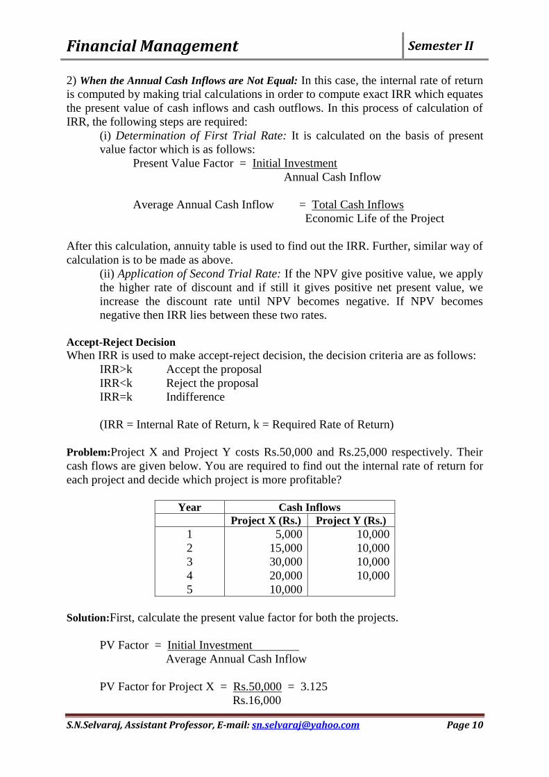
Problem:Project X and Project Y costs Rs.50,000 and Rs.25,000 respectively. Their

cash flows are given below. You are required to find out the internal rate of return for

each project and decide which project is more profitable?

Year Cash Inflows

Project X (Rs.) Project Y (Rs.)

1

2

3

4

5

5,000

15,000

30,000

20,000

10,000

10,000

10,000

10,000

10,000

Solution:First, calculate the present value factor for both the projects.

PV Factor = Initial Investment

Average Annual Cash Inflow

PV Factor for Project X = Rs.50,000 = 3.125

Rs.16,000



PV Factor for Project Y = Rs.25,000 = 2.5

Rs.10,000

The PV factor can be located in the Annuity Table. Present value for Project X for 5

years comes to 18% (present value for 5 years is 3.127, which is nearly equal to

3.125). Similarly for Project Y, it is 22% for 4 years.

Take 18% and 22% as discounting rate for Project X and Y. In this case, the present

value of Project X and Y is as follows: Computation of Present Value of Cash Inflow

Year Project X Project Y

PV

Factor at

18%

Cash

Inflow

(Rs)

Present

Value

(Rs.)

PV

Factor at

18%

Cash

Inflow (Rs)

Present

Value (Rs.)

1 0.847 5,000 4,235 0.820 10,000 8,200

2 0.718 15,000 10,770 0.672 10,000 6,720

3 0.609 30,000 18,270 0.551 10,000 5,510

4 0.516 20,000 10,320 0.451 10,000 4,510

5 0.437 10,000 4,370 - - - - 80,000 47,965 40,000 24,940

In order to equate the present values with the cash outlays of Rs.50,000 and Rs.25,000

for Project X and Project Y respectively, the IRR will have to be lower than 18% for

Project X and lower than 22% for project Y because the NPV is negative in both the

cases. So, we must consider second trial rate at a discount rate of 16% for X and 20%

for Y. The present values of these rates will be as follows:

Computation of Present Value of Cash Inflow

Year Project X Project Y

PV

Factor at

16%

Cash

Inflow

(Rs)

Present

Value

(Rs.)

PV

Factor at

20%

Cash

Inflow (Rs)

Present

Value (Rs.)

1 0.862 5,000 4,310 0.833 10,000 8,330

2 0.743 15,000 11,145 0.694 10,000 6,940

3 0.641 30,000 19,230 0.579 10,000 5,790

4 0.552 20,000 11,040 0.482 10,000 4,820

5 0.476 10,000 4,760 - - - -

80,000 50,485 40,000 25,880

Since the NPV of the both projects is positive, now apply the formula to calculate the

IRR.

IRR = X + Px−I (Y−X)

Px−Py

Where, X = Lower discount rate, Y = Higher discount rate,

Px = Present value of cash inflows at X,



Py =Present value of cash inflows at Y,

I = Initial investment.

IRR for Project X

= 16 + Rs.50,485−Rs.50,000 (18−16) = 16 + Rs.970 = 16.38%

Rs.50,485−Rs.47,965 Rs.2,520

IRR for Project Y

= 20 + Rs.25,880−Rs.25,000 (22−20) = 20 + Rs.1,760 = 21.87%

Rs.25,880−Rs.24,940 Rs.940

Hence, Project Y is more profitable than Project X because it shows a higher IRR.

The IRR acceptance rules are:

Accept the project when r> 0

Reject the project when r< 0

May accept the project when r = k

PROFITABILITY INDEX

Yet another time adjusted method of evaluating the investment proposals is the benefit

– cost (B/C) ratio or profitability index (PI). Profitability index is the ratio of the

present value of cash inflows, at the required rate of return, to the initial cash outflow

of the investment.

The formula for calculating benefit-cost ratio or profitability index is as follows:

PI = PV of cash inflows = PV(Ct)

Initial cash outlay C0

n

= ∑ (Ct)+ C0

t=1 (1+k)t

Problem

The initial cash outlay of project is Rs.100,000 and it can generate cash inflow of

Rs.40000, Rs.30000, Rs.50000 and Rs.20000 in year 1 through 4. Assume a 10

percent rate of discount. What is the PV of cash inflows at 10 percent discount rate?

Solution

PV = Rs.40000 (PVF1,0.10) + Rs.30000 (PVF2,0.10) + Rs.50000 (PVF3,0.10) +

Rs.20000 (PVF1,0.10)

= Rs.4000*0.909 + Rs.30000*0.826 + Rs.50000*0.751 + Rs.20000*0.683

= Rs.36360 + Rs.24780 + Rs.37550 + Rs.13660

NPV = Rs.112,350 – Rs.100,000 = Rs.12,350

PI = Rs.112350 / 100000 = 1.1235



Acceptance Rule

The following are the PI acceptance rules:

Accept the project when PI is greater than one PI > 1

Reject the project when PI is less than one PI < 1

May accept the project when PI is equal to one PI = 1

COMPARISON OF DCF TECHNIQUES

When two or more investment proposals are mutually exclusive, so that we can select

only one, ranking proposals on the basis of the IRR, NPV and PI methods may give

contradictory results. If projects are ranked differently using these methods, the

conflict in rankings will be due to one or a combination of the following three project

differences.

1) Scale of Investment : Costs of projects differ.

2) Cash flow Pattern : Timing of cash flows differs. For example, the cash

flows of

one project increase over time whereas those of

another decrease.

3) Project Life : Projects have unequal useful lives.

It is important to remember that one or more of these project differences constitutes a

necessary, but not sufficient, condition for a conflict in rankings. Thus, it is possible

that mutually exclusive projects could differ on all these dimensions (scale, pattern

and life) and still not show any conflict between rankings under the IRR, NPV and PI

methods.

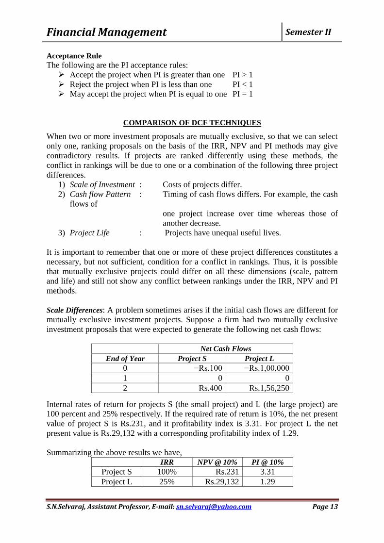
Scale Differences: A problem sometimes arises if the initial cash flows are different for

mutually exclusive investment projects. Suppose a firm had two mutually exclusive

investment proposals that were expected to generate the following net cash flows:

Internal rates of return for projects S (the small project) and L (the large project) are

100 percent and 25% respectively. If the required rate of return is 10%, the net present

value of project S is Rs.231, and it profitability index is 3.31. For project L the net

present value is Rs.29,132 with a corresponding profitability index of 1.29.

Summarizing the above results we have,

Net Cash Flows

End of Year Project S Project L

0 −Rs.100 −Rs.1,00,000

1 0 0

2 Rs.400 Rs.1,56,250

IRR NPV @ 10% PI @ 10%

Project S 100% Rs.231 3.31

Project L 25% Rs.29,132 1.29



Ranking the projects based on our results reveals,

Project S is preferred if we use either the internal rate of return or profitability index

method. However, project L is preferred if we use the net present value method. If we

can choose only one of these proposals, we obviously have a conflict.

Differences in Cash Flow Patterns: To illustrate the nature of the problem that may be

caused by differences in cash flow patterns, assume that a firm is facing two mutually

exclusive investment proposals with the following cash flow patterns:

Notice that both projects, D and I, require the same initial cash outflow and have the

same useful life. Their cash flow patterns, however, are different. Project D‟s cash

flows decrease over time, whereas Project I‟s cash flows increase.

IRR for projects D and I are 23% and 17% respectively. For every discount rate

greater than 10%, project D‟s net present value and profitability index will be larger

than those for project I.

On the other hand, for every discount rate less 10%, Project I‟s net present value and

profitability index will be larger than those for project D.

If we assume a required rate of return (k) of 10%, each project will have identical

NPV of Rs.198 and PI of 1.17. Using these results to determine project ranking we

find the following: k < 10% k > 10%

Rankings IRR NPV PI NPV PI

1st Place Project D I I D D

2nd

Place Project I D D I I

With the internal rate of return method, then, the implicit reinvestment rate will differ

from project to project depending on the pattern of the cash flow stream for each

proposal under consideration. For a project with a high internal rate of return, a high

reinvestment rate is assumed.

Ranking IRR NPV @ 10% PI @ 10%

1st Place S L S

2nd

Place L S L

Net Cash Flows

End of Year Project D Project I

0 −Rs.1,200 −Rs.1,200

1 1000 100

2 500 600

3 100 1,080



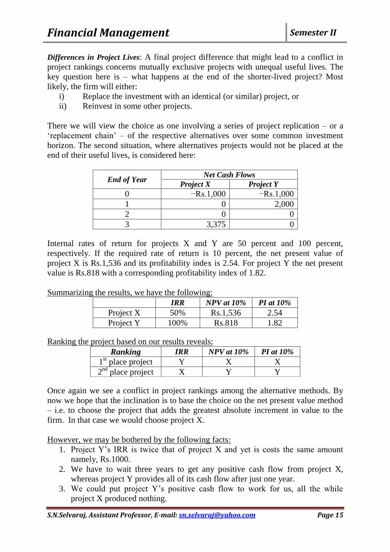
Differences in Project Lives: A final project difference that might lead to a conflict in

project rankings concerns mutually exclusive projects with unequal useful lives. The

key question here is – what happens at the end of the shorter-lived project? Most

likely, the firm will either:

i) Replace the investment with an identical (or similar) project, or

ii) Reinvest in some other projects.

There we will view the choice as one involving a series of project replication – or a

„replacement chain‟ – of the respective alternatives over some common investment

horizon. The second situation, where alternatives projects would not be placed at the

end of their useful lives, is considered here:

Internal rates of return for projects X and Y are 50 percent and 100 percent,

respectively. If the required rate of return is 10 percent, the net present value of

project X is Rs.1,536 and its profitability index is 2.54. For project Y the net present

value is Rs.818 with a corresponding profitability index of 1.82.

Summarizing the results, we have the following:

Ranking the project based on our results reveals:

Once again we see a conflict in project rankings among the alternative methods. By

now we hope that the inclination is to base the choice on the net present value method

– i.e. to choose the project that adds the greatest absolute increment in value to the

firm. In that case we would choose project X.

However, we may be bothered by the following facts:

1. Project Y‟s IRR is twice that of project X and yet is costs the same amount

namely, Rs.1000.

2. We have to wait three years to get any positive cash flow from project X,

whereas project Y provides all of its cash flow after just one year.

3. We could put project Y‟s positive cash flow to work for us, all the while

project X produced nothing.

End of Year Net Cash Flows

Project X Project Y

0 −Rs.1,000 −Rs.1,000

1 0 2,000

2 0 0

3 3,375 0

IRR NPV at 10% PI at 10%

Project X 50% Rs.1,536 2.54

Project Y 100% Rs.818 1.82

Ranking IRR NPV at 10% PI at 10%

1st place project Y X X

2nd

place project X Y Y



PROJECT SELECTION UNDER CAPITAL RATIONING

Capital rationingrefers to a situation where the firm is constrained for external or self-

imposed, reason to obtain necessary funds to invest in all investment projects with

positive NPV. Under capital rationing, the management not only has to simply

determine the profitable investment opportunities, but it has also to decide to obtain

that combination of the profitable projects which yields highest NPV within the

available funds.

Types of Capital Rationing

Hard Capital Rationing: Hard capital rationing refers to the existence of real

constraints, often tied to serious consideration such as sound financial

judgment or legal concerns.

Soft Capital Rationing: Soft capital rationing refers to the practice of placing

limits on the amount of funds available for the execution of projects, based on

the judgment of senior managers. Company mangers normally view this

practice as one method they can use to exercise financial control over the

company. Typically, the practice of soft rationing also includes a placement of

limits at the divisional or departmental level, commonly referred to as capital

budget allocation.

Causes for Capital Rationing

Capital rationing may arise due to external factors or internal constraints imposed by

the management. Thus there are two types of capital rationing.

External Capital Rationing

Internal Capital Rationing

External Causes of Capital Rationing: External capital rationing mainly occurs on

account of the imperfections in capital markets. Imperfections may be caused by

deficiencies in market information or by rigidities of attitude that hamper the free flow

of capital. The reason for this is difference in rates is the transaction costs. Because of

these imperfections, the firm is not able to obtain necessary capital to finance its

profitable investment opportunities.

Internal Causes of Capital Rationing:Internal capital rationing is caused by self-

imposed restrictions by the management. Various types of constraints may be

imposed. For example, it may be decided not to obtain additional funds by incurring

debt. This may be a part of the firm‟s conservative financial policy. Whatever may be

the type of restrictions, the implication is that some of the profitable projects will have

to be foregone because of the lack of funds.

It is quite difficult sometimes to justify the internal capital rationing. But generally it

is used as a means of financial control. A company may put investment limits if it

finds itself capable of coping with the strains and organizational problems of a fast

growth.



Methods of Capital Rationing

There are two important methods that are used for capital rationing:

(1) Ranking Method and

(2) Mathematical Programming Method.

Ranking Method:Under this method, the available projects are ranked according to a

chosen criterion (like NPV, IRR, PI, etc.). The project for which the value of the

chosen criterion is the highest (say highest NPV or highest IRR etc) is assigned the

top rank and the project with the next highest value of the chosen criterion follows

with rank-2 and so on.

After the projects are ranked, the projects are chosen starting from the top. This is a

simple method of capital rationing. However, this method suffers from two

deficiencies:

a) Investment Criterion: There are many different criteria (like NPV, IRR, IR, PI,

etc.) that are used for ranking the available projects. It is likely that different

investment criteria may give different results. There is no guarantee that the

same ranking for projects will be obtained irrespective of the criterion chosen

for ranking.

b) Project Indivisibility: Another problem that is encountered in using ranking

method arises due to indivisible nature of project investments. After the

available projects are ranked according to some criterion, choice of projects is

done starting from the project with the top rank and coming downwards in

ranking till the capital expenditure budget is exhausted. Since these projects are

indivisible in nature, this method of choosing the projects to match the capital

expenditure budget may sometimes give erroneous results.

Mathematical Programming Method:When the number of projects considered good

for investment increases, the number of feasible combinations of projects increases.

With increasing number of projects the issue of finding the optimum combination of

projects to suit the funds available for investment becomes a lengthy exercise.

The problem gets further involved as the number of years in the planning horizon

increases. Under such circumstances, choosing the optimum combination of projects

by first ranking all the projects according to some chosen investment criterion and

then studying all the feasible combination becomes a more laborious exercise.

Mathematical programming models are of use for handling such situations.

Mathematical programming models provide a methodology, which when followed

lead to the optimum combination of projects.

The following are two mathematical programming models useful for capital rationing:

1) Linear Programming Model: Linear programming is one of the widely to the

problem of optimum techniques for arriving at solution to the problem of

optimum utilization of limited resources. The linear programming models have

three elements, viz. Decision variable, Objective function and Constraints.



The linear programming model is based on the following assumptions:

a) The objective function and the constraint equations are linear.

b) All the coefficient in the objective function and constraint equations are

defined with certainty

c) The objective function is one-dimensional

d) The decision variables are considered to be continuous

e) Resources are homogeneous. This means if 100 hours of direct labour are

available, each of these hours is equally productive.

2) Integer Linear Programming Model: In this pioneering work on the application

of mathematical programming to capital budgeting, Weingarten discussed the

linear programming approach as well as the integer linear programming

approach. The principal motivation for the use of integer linear programming

approach is:

a) It overcomes the problem of partial projects which besets the linear

programming model because it permits only 0 to 1 value for the

decision variables.

b) It is capable of handling virtually any kind of project

interdependency.

c) The only difference between this integer linear programming model

and the basic linear programming model is that the integer linear

programming model ensures that a project is either completely

accepted or completely rejected.

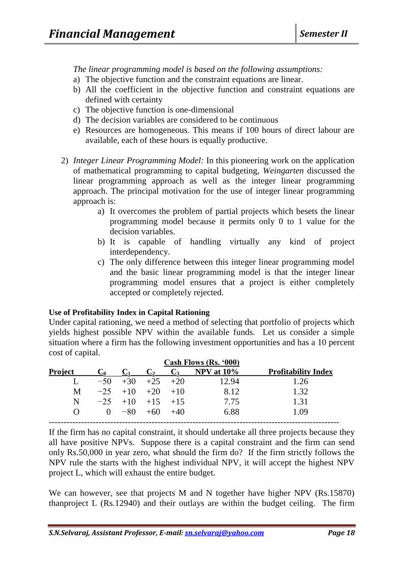
Use of Profitability Index in Capital Rationing

Under capital rationing, we need a method of selecting that portfolio of projects which

yields highest possible NPV within the available funds. Let us consider a simple

situation where a firm has the following investment opportunities and has a 10 percent

cost of capital. Cash Flows (Rs. ‘000)

Project C0 C1 C2 C3 NPV at 10% Profitability Index

L −50 +30 +25 +20 12.94 1.26

M −25 +10 +20 +10 8.12 1.32

N −25 +10 +15 +15 7.75 1.31

O 0 −80 +60 +40 6.88 1.09

---------------------------------------------------------------------------------------------------

If the firm has no capital constraint, it should undertake all three projects because they

all have positive NPVs. Suppose there is a capital constraint and the firm can send

only Rs.50,000 in year zero, what should the firm do? If the firm strictly follows the

NPV rule the starts with the highest individual NPV, it will accept the highest NPV

project L, which will exhaust the entire budget.

We can however, see that projects M and N together have higher NPV (Rs.15870)

thanproject L (Rs.12940) and their outlays are within the budget ceiling. The firm



should, therefore, undertake M and N rather than L to obtain the highest possible

NPV.

The capital budgeting procedure under the simple situation of capital rationing may be

summarized as follows:

The NPV rule should be modified while choosing among projects under

capital constraint.

The objective should be to maximize NPV per rupee of capital rather than to

maximize NPV.

Projects should be ranked by their profitability index and top-ranked projects

should be undertaken until funds are exhausted.

Programming Approach to Capital Rationing

The limitations of the profitability index method make it necessary to have a better

method for investment decisions under capital rationing. Let us develop a general

procedure for solving the capital rationing problem. Reconsider the example in which

we have two-period budget constraint. Our objective is to choose that package

projects, which gives us maximum total net present value subject to the firm‟s

resources.

Mathematical Programming Model: Consider the following four projects:

Project Net Present Value

(NPV)

Cash Outflow in

Year 1 (CF1)

Cash Outflow in

Year 2 (CF2)

L 12.94 50 −30

M 8.12 25 −10

N 7.75 25 −10

O 6.88 0 80

The total cash outlay in each of the two periods should not exceed Rs.50,000. The

investment in any project should not be negative and not to invest in more than one

each project. Maximize NPV by using programming method.

We can summarize the decision problem as follows:

Maximize

12.94 XL + 8.12 XM + 7.75 XN + 6.88 XO

Subject to

50 XL + 25 XM + 25 XN + 0 XO ≤ 50

−30 XL −10 XM −10 XN + 80 XO ≤ 50

0 ≤ XL ≤ 1

0 ≤ XM ≤ 1

0 ≤ XN ≤ 1

0 ≤ XO ≤ 1

It may be realized that the above situation is a linear programming (LP) problem. It

can be easily solved with the help of a computer (in Excel). Using the LP model, the

computer tells us that we should accept Projects M and N entirely and a fraction equal



to 0.875 of Project O; Project L should be rejected. This is the optimal solution and

we shall obtain a maximum NPV equal to:

12.94*0+8.12*1+7.75*1+6.88*0.875 = 21.89 or Rs 21890

Capital Rationing in Practice

How serious is the problem of capital rationing in practice? Do companies reject

projects due to shortage of funds? How do they select projects under capital rationing?

Capital rationing does not seem to be a serious problem in problem. It may arise due

to the internal constraint or the management‟s reluctance to raise external funds.

When companies face the problem of shortage of funds, they use simple rules of

choosing projects rather than the complicated mathematical models.

INFLATION AND CAPITAL BUDGETING

Inflation is a monetary ailment in an economy and it can be defined as “the change in

purchasing power in a currency from period to period relative to some basket of goods

and services”. When analyzing capital budgeting decisions with inflation, it is

required to distinguish between expected and unexpected inflation. Expected inflation

refers to the loss the manager anticipates in buying power overtime whereas

unexpected inflation refers to the difference between actual and expected inflation.

Typically, the non-financial manager has two options in dealing with a capital

budgeting situation with inflation:

1) Restate the cash flows in nominal terms and discount them at a nominal cost of

capital (minimum required rate of return).

2) Restate both the cash flows and cost of capital in constant terms and discount

the constant cash flows at a constant cost of capital.

Inflation and Cash Flows

Estimating the cash flows is the first step which requires the estimation of cost and

benefits of different proposals being considered for decision-making. Usually two

alternatives are suggested for measuring the „Cost and benefit of a proposal‟ i.e. the

accounting profits and the cashflows.

In reality, estimating the cash flows is most important as well as difficult task. It is

because of uncertainty and accounting ambiguity. Accounting profit is the resultant

figure on the basis of several accounting concepts and policies. Adequate care should

be taken while adjusting the accounting data, otherwise errors would arise in

estimating cash flows.

Implications of Expected Rate of Inflation on the Capital Budgeting

It is noted from the above analysis; effects of inflation significantly influence the

capital budgeting decision making process. If the prices of outputs and the discount

rates are expected to rise at the same rate, capital budgeting decision will not be

neutral.



The implications of expected rate of inflation on the capital budgeting process and

decision-making are as follows:

1) The company should raise the output price above the expected rate of inflation,

unless it has lower NPV which may lead to forego the proposals and vice versa.

2) If the company is unable to raise the output price, it can make some internal

adjustments through careful management of working capital.

3) With respect of discount rate, the adjustment should be made through capital

structure.

CONCEPT AND MEASUREMENT OF COST OF CAPITAL

The term cost of capital refers to the minimum rate of return a firm must earn on its

investment so that the market value of the company‟s equity shares does not fall. This

is in consonance with the overall firm‟s objective of wealth maximization. In other

words, cost of capital of a firm is the minimum rate of return expected by its investors.

It is the weighted average cost of various sources of finance used by a firm. It is also

referred to as cut-off rate, target cost, hurdle cost, minimum rate of return and

standard cost.

According to Solomon Ezra, “Cost of Capital is the minimum required rate of earning

or the cut-off rate of capital expenditures”.

According to Hampton, John J, “The rate of return the firm requires from investment in

order to increase the value of the firm in the market place”.

Significance of Cost of Capital

We should recognize that the cost of capital is one of the most difficult and disputed

topics in the finance theory. Financial experts express conflicting opinions as to the

correct way in which the cost of capital can be measured. Irrespective of the

measurement problems, it is concept of vital importance in the financial decision-

making. It is useful as a standard for:

Evaluating investment decisions

Designing a firm‟s debt policy and

Appraising the financial performance of top management

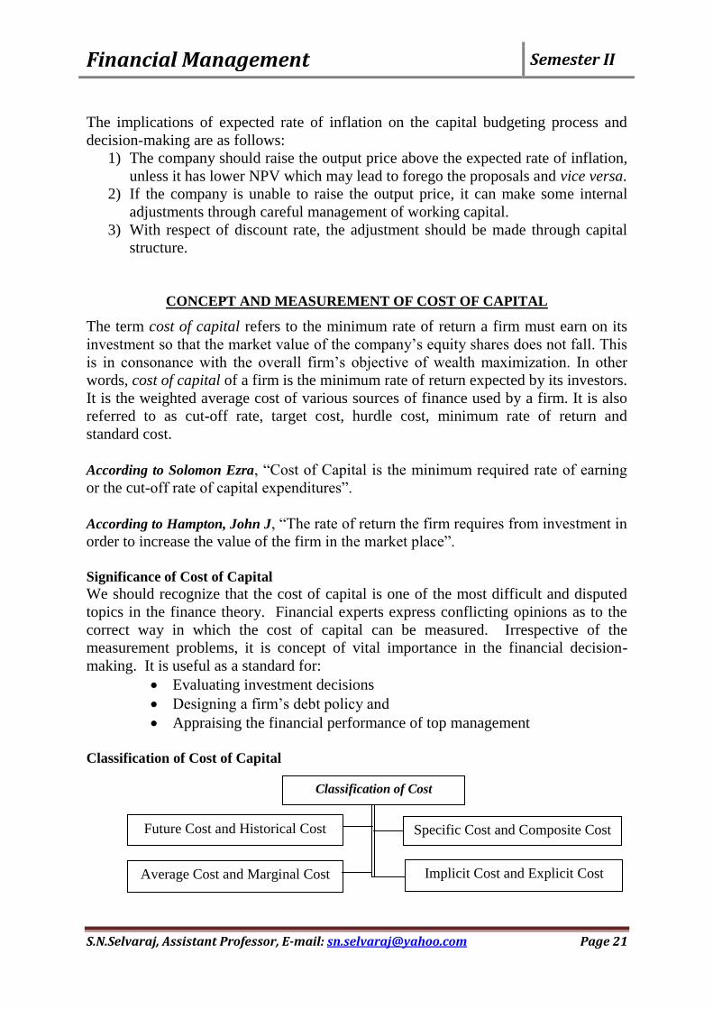
Classification of Cost of Capital

Classification of Cost

Future Cost and Historical Cost Specific Cost and Composite Cost

Average Cost and Marginal Cost Implicit Cost and Explicit Cost



Factors Affecting Cost of Capital

Factors affecting cost of capital are the elements in business environment that cause a

company‟s cost of capital to be high or low.

a) General Economic Conditions:

b) Market Conditions:

c) Firm‟s Operation and Financing Decisions: d) Amount of Financing

MEASUREMENT OF COST OF CAPITAL

For measuring cost of capital of the firm, it is essential to consider the different

sources from which the funds are received by the firm. In includes debt financing,

preference shares, retained earnings and equity capital, etc. The cost of each

component of capital has its cost called specific cost of capital. When these are

combined or total effects of cost for procurement of such capital from different

sources is called as overall or weighted average cost of capital.

Accordingly, the measurement of cost of capital is on the basis of either one of the

following:

(1) Measurement of cost of specific sources as shown in the figure.

(2) Measurement of overall/weighted average/composite cost of capital.

SPECIFIC COST AND OVERALL COST OF CAPITAL

COST OF DEBT/DEBENTURES

Cost of debt is the contractual rate of interest or coupon rate payable on debt. Debt

may be issued at par, at premium or discount. It may be perpetual or redeemable.

Debt Issued at Par

The before-tax cost of debt is the rate of return required by lenders. It is easy to

compute before-tax cost of debt issued and to be redeemed at par; it is simply equal to

the contractual (or coupon) rate of interest.

For example, a company decides to sell a new issue of 7 year 15 percent bonds of

Rs.100 each at par. If the company realizes the full face value of Rs.100 bond and

will pay Rs.100 principal to bondholders at maturity, the before-tax cost of debt will

simply be equal to the rate of interest of 15 percent. Thus:

kd = i = INT / B0

Measurement of Costs of

Specific Sources

Cost of Debt/Debentures Cost of Preference Shares

Cost of Equity Shares

Cost of Retained Earnings



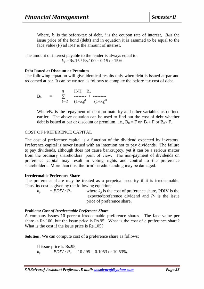
Where, kd is the before-tax of debt, i is the coupon rate of interest, B0is the

issue price of the bond (debt) and in equation it is assumed to be equal to the

face value (F) ad INT is the amount of interest.

The amount of interest payable to the lender is always equal to:

kd =Rs.15 / Rs.100 = 0.15 or 15%

Debt Issued at Discount or Premium

The following equation will give identical results only when debt is issued at par and

redeemed at par. It can be written as follows to compute the before-tax cost of debt.

n INTt Bn

B0 = ∑ -------- + ---------

t=1 (1+kd)t (1+kd)

n

WhereBn is the repayment of debt on maturity and other variables as defined

earlier. The above equation can be used to find out the cost of debt whether

debt is issued at par or discount or premium. i.e., B0 = F or B0> F or B0< F.

COST OF PREFERENCE CAPITAL

The cost of preference capital is a function of the dividend expected by investors.

Preference capital is never issued with an intention not to pay dividends. The failure

to pay dividends, although does not cause bankruptcy, yet it can be a serious matter

from the ordinary shareholders‟ point of view. The non-payment of dividends on

preference capital may result in voting rights and control to the preference

shareholders. More than this, the firm‟s credit standing may be damaged.

Irredeemable Preference Share

The preference share may be treated as a perpetual security if it is irredeemable.

Thus, its cost is given by the following equation:

kp = PDIV / P0 where kp is the cost of preference share, PDIV is the

expectedpreference dividend and P0 is the issue

price of preference share.

Problem: Cost of Irredeemable Preference Share

A company issues 10 percent irredeemable preference shares. The face value per

share is Rs.100, but the issue price is Rs.95. What is the cost of a preference share?

What is the cost if the issue price is Rs.105?

Solution: We can compute cost of a preference share as follows:

If issue price is Rs.95,

kp = PDIV / P0 = 10 / 95 = 0.1053 or 10.53%



If issue price is Rs.105,

kp = PDIV / P0 = 10 / 105 = 0.0952 or 9.52%

Redeemable Preference Share

Redeemable preference shares (that is, preference shares with finite maturity) are also

issued in practice. A formula similar to the above equation can be used to compute

the cost of redeemable preference share:

n PDIVt Pn

P0 = ∑ --------- + -------

t=1 (1+kp)t (1+kp)

n

The cost of preference share is not adjusted for taxes because preference dividend is

paid after the corporate taxes have been paid. Preference dividends do not save any

taxes. Thus, the cost of preference share is automatically computed on the after-tax

basis. Since interest is tax deductible and preference dividend is not, the after-tax cost

of preference share is substantially higher than the after-tax cost of debt.

COST OF EQUITY CAPITAL

Firms may raise equity capital internally by retaining earnings. Alternatively, they

could distribute the entire earnings to equity shareholders and raise equity capital

externally by issuing new shares. In both cases, shareholders are providing funds to

the firms to finance their capital expenditures. Therefore, the equity shareholders‟

required rate of return would be the same whether they supply funds by purchasing

new shares or by foregoing dividends, which could have been distributed to them.

The firm may have to issue new shares at a price lower than the current market price.

Also it may have to incur flotation costs. Thus, external equity will cost more to the

firm than the internal equity.

Cost of Internal Equity:The Dividend-growth Model

A firm‟s internal equity consists of its retained earnings. The opportunity cost of the

retained earnings is the rate of return foregone by equity shareholders. The

shareholders generally expect dividend and capital gain from their investment. The

required rate of return of shareholders can be determined from the dividend valuation

model.

Normal Growth:The dividend-valuation model for a firm whose dividends are

expected to grow at a constant rate of g is as follows:

P0 = DIV1 / ke – g where DIV1 = DIV0 (1+g)

The above equation can be solved for calculating the cost of equity ke as follows:

ke = DIV1 / P0 + g

The cost of equity is, thus, equal to the expected dividend yield (DIV1 / P0) plus

capital gain rate as reflected by expected growth in dividends (g). It may be noted that

equation is based on the following assumptions:



The market price of the ordinary share, P0 , is a function of expected

dividends.

The dividend, DIV1, is positive (i.e., DIV1> 0)

The dividends grow at a constant growth rate g, and the growth rate is

equal to the return on equity, ROE, times the retention ratio, b (i.e., g =

ROE*b)

The dividend payout ratio (i.e., (1–b) is constant.

The cost of retained earnings determined by the dividend-valuation model implies that

if the firm would have distributed earnings to shareholders, they could have invested it

in the shares of the firm or in the share of other firms of similar risk at the market

price (P0) to earn a rate of return equal to ke. Thus, the firm should earn a return on

retained funds equal to ke to ensure growth of dividends and share price. If a return

less than ke is earned on retained earnings, the market price of the firm‟s share will

fall. It may be emphasized again that the cost of retained earnings will be equal to the

shareholders‟ required rate of return since no flotation costs are involved.

Problem: Constant-Growth Model and the Cost of Equity

Suppose that the current market price of a company‟s share is Rs.90 and the expected

dividend per share next year is Rs.4.50. If the dividends are expected to grow at a

constant rate of 8 percent, what will be the shareholders‟ required rate of return?

Solution: The share holders‟ required rate of return is,

ke = DIV1 / P0 + g

= Rs.4.50 / Rs.90 + 0.08

= 0.05 + 0.08 = Rs.0.13 or 13%

If the company intends to retain earnings, it should at least earn a return of 13 percent

on retained earnings to keep the current market price unchanged.

Zero-growthIn addition to its use in constant and variable growth situations, the

dividend valuation model can also be used to estimate the cost of equity of no-growth

companies. The cost of equity of a share on which a constant amount of dividend is

expected perpetually is given as follows:

ke = DIV1 / P0

The growth rate g will be zero if the firm does not retain any of its earnings; that is,

the firm follows a policy of 100 percent payout. Under such case, dividends will be

equal to earnings and therefore equation can also be written as:

ke = DIV1 / P0 = EPS1 / P0 (since g = 0)

which implies that in a no-growth situation, the expected earnings-price (E/P) ratio

may be used as the measure of the firm‟s cost of equity.

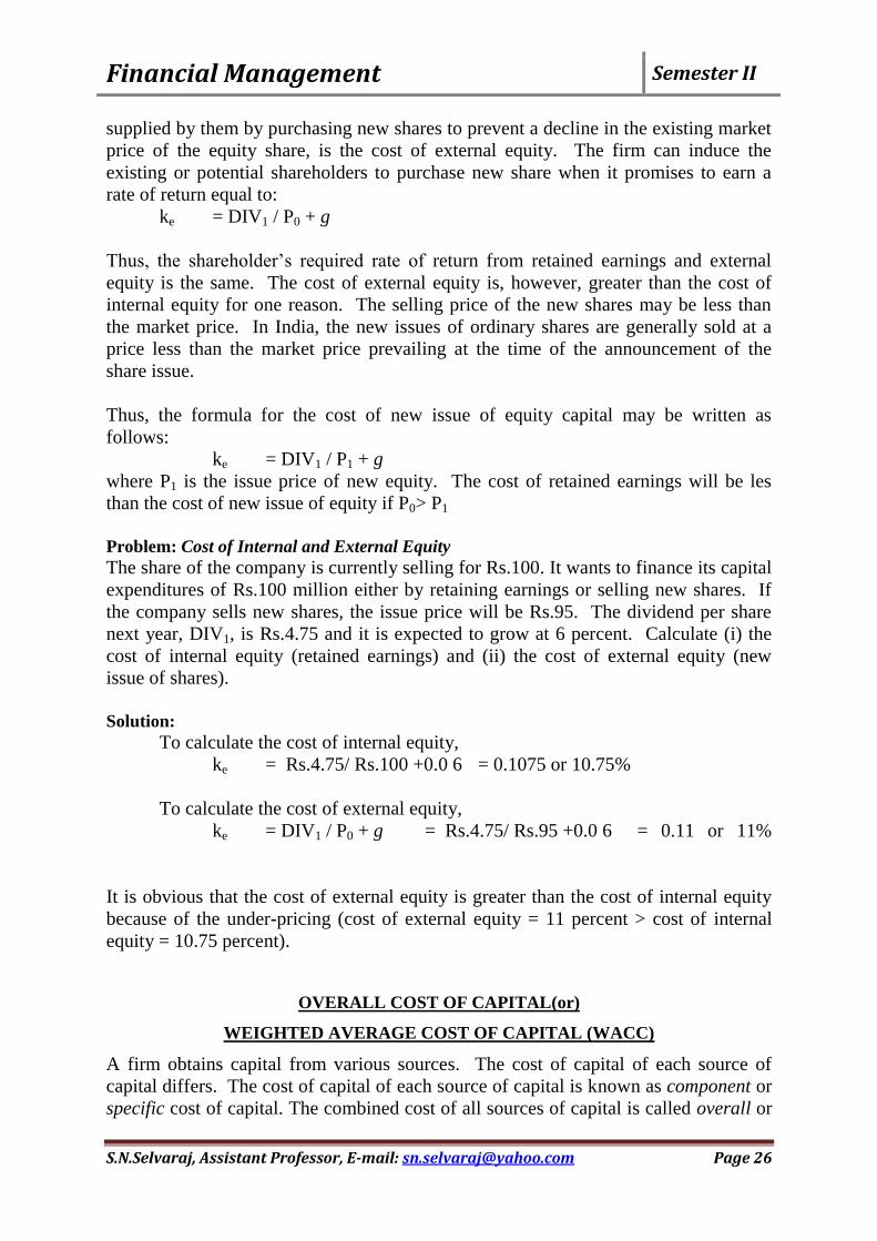
Cost of External Equity: The Dividend-growth Model

The firm‟s external equity consists of funds raised externally through public or right

issues. The minimum rate of return, which the equity shareholders require on funds



supplied by them by purchasing new shares to prevent a decline in the existing market

price of the equity share, is the cost of external equity. The firm can induce the

existing or potential shareholders to purchase new share when it promises to earn a

rate of return equal to:

ke = DIV1 / P0 + g

Thus, the shareholder‟s required rate of return from retained earnings and external

equity is the same. The cost of external equity is, however, greater than the cost of

internal equity for one reason. The selling price of the new shares may be less than

the market price. In India, the new issues of ordinary shares are generally sold at a

price less than the market price prevailing at the time of the announcement of the

share issue.

Thus, the formula for the cost of new issue of equity capital may be written as

follows:

ke = DIV1 / P1 + g

where P1 is the issue price of new equity. The cost of retained earnings will be les

than the cost of new issue of equity if P0> P1

Problem: Cost of Internal and External Equity

The share of the company is currently selling for Rs.100. It wants to finance its capital

expenditures of Rs.100 million either by retaining earnings or selling new shares. If

the company sells new shares, the issue price will be Rs.95. The dividend per share

next year, DIV1, is Rs.4.75 and it is expected to grow at 6 percent. Calculate (i) the

cost of internal equity (retained earnings) and (ii) the cost of external equity (new

issue of shares).

Solution:

To calculate the cost of internal equity,

ke = Rs.4.75/ Rs.100 +0.0 6 = 0.1075 or 10.75%

To calculate the cost of external equity,

ke = DIV1 / P0 + g = Rs.4.75/ Rs.95 +0.0 6 = 0.11 or 11%

It is obvious that the cost of external equity is greater than the cost of internal equity

because of the under-pricing (cost of external equity = 11 percent > cost of internal

equity = 10.75 percent).

OVERALL COST OF CAPITAL(or)

WEIGHTED AVERAGE COST OF CAPITAL (WACC)

A firm obtains capital from various sources. The cost of capital of each source of

capital differs. The cost of capital of each source of capital is known as component or

specific cost of capital. The combined cost of all sources of capital is called overall or



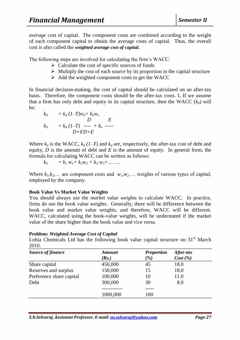
average cost of capital. The component costs are combined according to the weight

of each component capital to obtain the average costs of capital. Thus, the overall

cost is also called the weighted average cost of capital.

The following steps are involved for calculating the firm‟s WACC:

Calculate the cost of specific sources of funds

Multiply the cost of each source by its proportion in the capital structure

Add the weighted component costs to get the WACC

In financial decision-making, the cost of capital should be calculated on an after-tax

basis. Therefore, the component costs should be the after-tax costs. L If we assume

that a firm has only debt and equity in its capital structure, then the WACC (k0) will

be:

k0 = kd (1–T)wd+ kewe

D E

k0 = kd (1–T) ---- + ke -----

D+ED+E

Where k0 is the WACC, kd (1–T) and kd are, respectively, the after-tax cost of debt and

equity, D is the amount of debt and E is the amount of equity. In general form, the

formula for calculating WACC can be written as follows:

k0 = k1 w1+ k2w2 + k3 w3+……..

Where k1,k2,… are component costs and w1,w2…. weights of various types of capital,

employed by the company.

Book Value Vs Market Value Weights

You should always use the market value weights to calculate WACC. In practice,

firms do use the book value weights. Generally, there will be difference between the

book value and market value weights, and therefore, WACC will be different.

WACC, calculated using the book-value weights, will be understated if the market

value of the share higher than the book value and vice versa.

Problem: Weighted Average Cost of Capital

Lohia Chemicals Ltd has the following book value capital structure on 31st March

2010.

Source of finance Amount Proportion After-tax

(Rs.) (%) Cost (%)

Share capital 450,000 45 18.0

Reserves and surplus 150,000 15 18.0

Preference share capital 100,000 10 11.0

Debt 300,000 30 8.0

------------ -----

1000,000 100



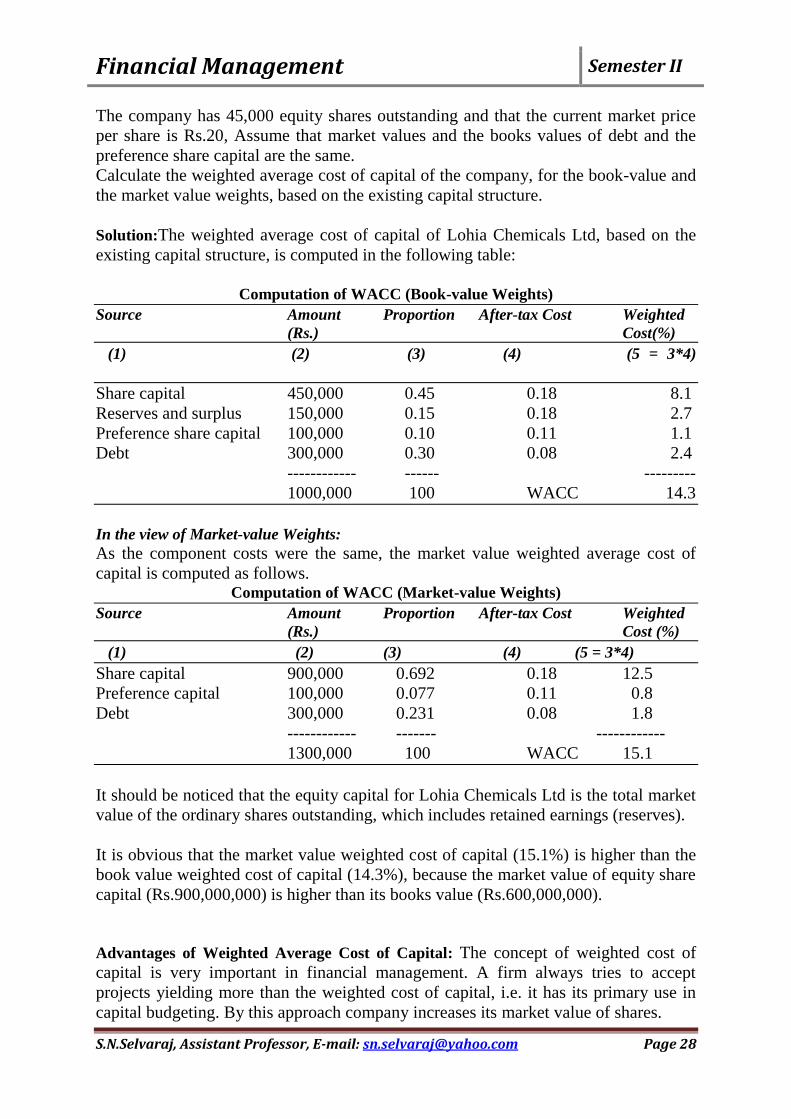
The company has 45,000 equity shares outstanding and that the current market price

per share is Rs.20, Assume that market values and the books values of debt and the

preference share capital are the same.

Calculate the weighted average cost of capital of the company, for the book-value and

the market value weights, based on the existing capital structure.

Solution:The weighted average cost of capital of Lohia Chemicals Ltd, based on the

existing capital structure, is computed in the following table:

Computation of WACC (Book-value Weights)

Source Amount Proportion After-tax Cost Weighted

(Rs.) Cost(%)

(1) (2) (3) (4) (5 = 3*4)

Share capital 450,000 0.45 0.18 8.1

Reserves and surplus 150,000 0.15 0.18 2.7

Preference share capital 100,000 0.10 0.11 1.1

Debt 300,000 0.30 0.08 2.4

------------ ------ ---------

1000,000 100 WACC 14.3

In the view of Market-value Weights:

As the component costs were the same, the market value weighted average cost of

capital is computed as follows. Computation of WACC (Market-value Weights)

Source Amount Proportion After-tax Cost Weighted

(Rs.) Cost (%)

(1) (2) (3) (4) (5 = 3*4)

Share capital 900,000 0.692 0.18 12.5

Preference capital 100,000 0.077 0.11 0.8

Debt 300,000 0.231 0.08 1.8

------------ ------- ------------

1300,000 100 WACC 15.1

It should be noticed that the equity capital for Lohia Chemicals Ltd is the total market

value of the ordinary shares outstanding, which includes retained earnings (reserves).

It is obvious that the market value weighted cost of capital (15.1%) is higher than the

book value weighted cost of capital (14.3%), because the market value of equity share

capital (Rs.900,000,000) is higher than its books value (Rs.600,000,000).

Advantages of Weighted Average Cost of Capital: The concept of weighted cost of

capital is very important in financial management. A firm always tries to accept

projects yielding more than the weighted cost of capital, i.e. it has its primary use in

capital budgeting. By this approach company increases its market value of shares.



1) Straight-Forward and Logical:

2) Builds on Individual Debt and Equity Components: 3) Accurate in Periods of Normal Profits: 4) Accurate when the Debt Level is Reasonable:

Text Books

1. M.Y.Khan and P.K.Jain, “Financial Management” Tata McGraw Hill, 6th

Edition, 2011.

2. I.M.Pandey, “Financial Management” Vikas Publishing House Pvt. Ltd., 10th

Education 2012. References

1. AswatDamodaran, Corporate Finance Theory and Practice, John Wiley &

Sons, 2011.

2. James C Vanhorne, Fundamentals of Financial Management, PHI Learning,

11th

Edition, 2012.

3. Brigham Ehrhardt, Financial Management Theory and Practice, Cengage

Learning, 12th

Edition, 2010.

4. Prasanna Chandra, Financial Management, Tata McGraw Hill, 9th

Edition,

2012.

5. Srivatsava, Mishra, Financial Management, Oxford University Press, 2011.

Ba7202 financial management (unit2) notes

Education

Transcript of Ba7202 financial management (unit2) notes