BA552-Week3
83
2-1 Zappos Key issues: Increasing customer service They defined customer service as their core competency of their firm High cost of customer service Zappos responses: Relocating to Las Vegas Employee training and hiring program
-
Upload
reza-mohagi -
Category
Documents
-
view
2 -
download
0
description
Logistics
Transcript of BA552-Week3

2-1
Zappos
Key issues:Increasing customer serviceThey defined customer service as their core
competency of their firmHigh cost of customer service
Zappos responses:Relocating to Las VegasEmployee training and hiring program

2-2
Inventory driven Costs Key issues:
Turning a dollarShort life cycle of productsComponent devaluation costsPrice protection costsProduct return costsObsolescence costs
HP responses:Using a one stage supply chainSingle central factoryAirfreight to customers

McGraw-Hill/Irwin Copyright © 2008 by The McGraw-Hill Companies, Inc. All rights reserved.
Chapter 2
InventoryManagementand Risk Pooling

2-4
2.1 IntroductionWhy Is Inventory Important?
Distribution and inventory (logistics) costs are quite substantial
Total U.S. Manufacturing Inventories ($m): 1992-01-31: $m 808,773 1996-08-31: $m 1,000,774 2006-05-31: $m 1,324,108
Inventory-Sales Ratio (U.S. Manufacturers): 1992-01-01: 1.56 2006-05-01: 1.25

2-5
Why Is Inventory Required?
Uncertainty in customer demandShorter product lifecyclesMore competing products
Uncertainty in suppliesQuality/Quantity/Costs/Delivery Times
Delivery lead times Incentives for larger shipments

2-6
Inventory Management-Demand Forecasts
Uncertain demand makes demand forecast critical for inventory related decisions:What to order?When to order?How much is the optimal order quantity?
Approach includes a set of techniquesINVENTORY POLICY!!

2-7
Supply Chain Factors in Inventory Policy
Estimation of customer demand Replenishment lead time The number of different products being considered The length of the planning horizon Costs
Order cost: Product cost Transportation cost
Inventory holding cost, or inventory carrying cost: State taxes, property taxes, and insurance on inventories Maintenance costs Obsolescence cost Opportunity costs
Service level requirements

2-8
2.2.1. Economic Lot Size Model
FIGURE 2-3: Inventory level as a function of time

2-9
Assumptions
D items per day: Constant demand rate Q items per order: Order quantities are fixed, i.e., each
time the warehouse places an order, it is for Q items. K, fixed setup cost, incurred every time the warehouse
places an order. h, inventory carrying cost accrued per unit held in
inventory per day that the unit is held (also known as, holding cost)
Lead time = 0 (the time that elapses between the placement of an order and its receipt)
Initial inventory = 0 Planning horizon is long (infinite).

2-10
EOQ: Costs
FIGURE 2-4: Economic lot size model: total cost per unit time

2-11
Deriving EOQ
Total cost at every cycle:
Average inventory holding cost in a cycle: Q/2
Cycle time T =Q/D Average total cost per unit time:
2
hTQK
2
hQ
Q
KD
h
KDQ
2*

2-12
2.2.2. Demand Uncertainty
The forecast is always wrong It is difficult to match supply and demand
The longer the forecast horizon, the worse the forecast It is even more difficult if one needs to predict
customer demand for a long period of time Aggregate forecasts are more accurate.
More difficult to predict customer demand for individual SKUs
Much easier to predict demand across all SKUs within one product family

2-13
2.2.5. Multiple Order Opportunities
REASONS To balance annual inventory holding costs and annual fixed order
costs. To satisfy demand occurring during lead time. To protect against uncertainty in demand.
TWO POLICIES Continuous review policy
inventory is reviewed continuously an order is placed when the inventory reaches a particular level or reorder point. inventory can be continuously reviewed (computerized inventory systems are
used)
Periodic review policy inventory is reviewed at regular intervals appropriate quantity is ordered after each review. it is impossible or inconvenient to frequently review inventory and place orders if
necessary.

2-14
2.2.6. Continuous Review Policy Daily demand is random and follows a normal distribution. Every time the distributor places an order from the
manufacturer, the distributor pays a fixed cost, K, plus an amount proportional to the quantity ordered.
Inventory holding cost is charged per item per unit time. Inventory level is continuously reviewed, and if an order is
placed, the order arrives after the appropriate lead time. If a customer order arrives when there is no inventory on
hand to fill the order (i.e., when the distributor is stocked out), the order is lost.
The distributor specifies a required service level.

2-15
AVG = Average daily demand faced by the distributor
STD = Standard deviation of daily demand faced by the distributor
L = Replenishment lead time from the supplier to the
distributor in days h = Cost of holding one unit of the product for
one day at the distributor α = service level. This implies that the probability
of stocking out is 1 - α
Continuous Review Policy

2-16
(Q,R) policy – whenever inventory level falls to a reorder level R, place an order for Q units
What is the value of R?
Continuous Review Policy

2-17
Continuous Review Policy
Average demand during lead time: L x AVG
Safety stock:
Reorder Level, R:
Order Quantity, Q:
LSTDz
LSTDzAVGL
h
AVGKQ
2

2-18
Inventory Level Over Time
LSTDz Inventory level before receiving an order =
Inventory level after receiving an order =
Average Inventory =
LSTDzQ
LSTDzQ 2
FIGURE 2-9: Inventory level as a function of time in a (Q,R) policy

2-19
Service Level & Safety Factor, z
Service Level
90% 91% 92% 93% 94% 95% 96% 97% 98% 99% 99.9%
z 1.29 1.34 1.41 1.48 1.56 1.65 1.75 1.88 2.05 2.33 3.08
z is chosen from statistical tables to ensure that the probability of stockouts during lead time is exactly 1 - α

2-20
Continuous Review Policy Example
A distributor of TV sets that orders from a manufacturer and sells to retailers
Fixed ordering cost = $4,500Cost of a TV set to the distributor = $250Annual inventory holding cost = 18% of
product costReplenishment lead time = 2 weeksExpected service level = 97%

2-21
Month Sept Oct Nov. Dec. Jan. Feb. Mar. Apr. May June July Aug
Sales 200 152 100 221 287 176 151 198 246 309 98 156
Continuous Review Policy Example
Average monthly demand = 191.17 Standard deviation of monthly demand = 66.53
Average weekly demand = Average Monthly Demand/4.3Standard deviation of weekly demand = Monthly standard deviation/√4.3

2-22
Parameter Average weekly demand
Standard deviation of weekly demand
Average demand during lead time
Safety stock
Reorder point
Value 44.58 32.08 89.16 86.20 176
87.052
25018.0
Weekly holding cost =
Optimal order quantity = 67987.
58.44500,42
Q
Average inventory level = 679/2 + 86.20 = 426
Continuous Review Policy Example

2-23
Average lead time, AVGL Standard deviation, STDL. Reorder Level, R:
222 STDLAVGSTDAVGLzAVGLAVGR
2.2.7. Variable Lead Times
222 STDLAVGSTDAVGLz Amount of safety stock=
h
AVGKQ
2Order Quantity =

2-24
Inventory level is reviewed periodically at regular intervals
An appropriate quantity is ordered after each review Two Cases:
Short Intervals (e.g. Daily) Define two inventory levels s and S During each inventory review, if the inventory position falls below s,
order enough to raise the inventory position to S. (s, S) policy
Longer Intervals (e.g. Weekly or Monthly) May make sense to always order after an inventory level review. Determine a target inventory level, the base-stock level During each review period, the inventory position is reviewed Order enough to raise the inventory position to the base-stock level. Base-stock level policy
2.2.8. Periodic Review Policy

2-25
(s,S) policy
Calculate the Q and R values as if this were a continuous review model
Set s equal to RSet S equal to R+Q.

2-26
Base-Stock Level Policy Determine a target inventory level, the base-
stock level Each review period, review the inventory
position is reviewed and order enough to raise the inventory position to the base-stock level
Assume:r = length of the review periodL = lead time AVG = average daily demand STD = standard deviation of this daily demand.

2-27
Average demand during an interval of r + L days=
Safety Stock= LrSTDz
AVGLr )(
Base-Stock Level Policy

2-28
Base-Stock Level Policy
FIGURE 2-10: Inventory level as a function of time in a periodic review policy

2-29
Assume: distributor places an order for TVs every 3 weeks Lead time is 2 weeks Base-stock level needs to cover 5 weeks
Average demand = 44.58 x 5 = 222.9 Safety stock = Base-stock level = 223 + 136 = 359 Average inventory level =
Distributor keeps 5 (= 203.17/44.58) weeks of supply.
Base-Stock Level Policy Example
58.329.1
17.203508.329.1258.443

2-30
Optimal inventory policy assumes a specific service level target.
What is the appropriate level of service? May be determined by the downstream
customerRetailer may require the supplier, to maintain a
specific service levelSupplier will use that target to manage its own
inventoryFacility may have the flexibility to choose the
appropriate level of service
2.2.9. Service Level Optimization

2-31
Service Level Optimization
FIGURE 2-11: Service level inventory versus inventory level as a function of lead time

2-32
Trade-Offs
Everything else being equal:the higher the service level, the higher the
inventory level. for the same inventory level, the longer the
lead time to the facility, the lower the level of service provided by the facility.
the lower the inventory level, the higher the impact of a unit of inventory on service level and hence on expected profit

2-33
Retail Strategy
Given a target service level across all products determine service level for each SKU so as to maximize expected profit.
Everything else being equal, service level will be higher for products with:high profit marginhigh volumelow variabilityshort lead time

2-34
Profit Optimization and Service Level
FIGURE 2-12: Service level optimization by SKU

2-35
Target inventory level = 95% across all products.
Service level > 99% for many products with high profit margin, high volume and low variability.
Service level < 95% for products with low profit margin, low volume and high variability.
Profit Optimization and Service Level

2-36
2.3 Risk Pooling
Demand variability is reduced if one aggregates demand across locations.
More likely that high demand from one customer will be offset by low demand from another.
Reduction in variability allows a decrease in safety stock and therefore reduces average inventory.

2-37
Demand Variation
Standard deviation measures how much demand tends to vary around the averageGives an absolute measure of the variability
Coefficient of variation is the ratio of standard deviation to average demandGives a relative measure of the variability,
relative to the average demand

2-38
Acme Risk Pooling Case Electronic equipment manufacturer and distributor 2 warehouses for distribution in New York and New
Jersey (partitioning the northeast market into two regions)
Customers (that is, retailers) receiving items from warehouses (each retailer is assigned a warehouse)
Warehouses receive material from Chicago Current rule: 97 % service level Each warehouse operate to satisfy 97 % of demand
(3 % probability of stock-out)

2-39
Replace the 2 warehouses with a single warehouse (located some suitable place) and try to implement the same service level 97 %
Delivery lead times may increase But may decrease total inventory investment
considerably.
New Idea

2-40
Historical Data
PRODUCT A
Week 1 2 3 4 5 6 7 8
Massachusetts 33 45 37 38 55 30 18 58
New Jersey 46 35 41 40 26 48 18 55
Total 79 80 78 78 81 78 36 113
PRODUCT B
Week 1 2 3 4 5 6 7 8
Massachusetts 0 3 3 0 0 1 3 0
New Jersey 2 4 3 0 3 1 0 0
Total 2 6 3 0 3 2 3 0

2-41
Summary of Historical DataStatistics Product Average Demand Standard
Deviation of Demand
Coefficient of Variation
Massachusetts A 39.3 13.2 0.34
Massachusetts B 1.125 1.36 1.21
New Jersey A 38.6 12.0 0.31
New Jersey B 1.25 1.58 1.26
Total A 77.9 20.71 0.27
Total B 2.375 1.9 0.81

2-42
Inventory LevelsProduct Average
Demand During Lead Time
Safety Stock Reorder Point
Q
Massachusetts A 39.3 25.08 65 132
Massachusetts B 1.125 2.58 4 25
New Jersey A 38.6 22.8 62 31
New Jersey B 1.25 3 5 24
Total A 77.9 39.35 118 186
Total B 2.375 3.61 6 33

2-43
The higher the coefficient of variation, the greater the benefit from risk pooling The higher the variability, the higher the safety stocks
kept by the warehouses. The variability of the demand aggregated by the single warehouse is lower
The benefits from risk pooling depend on the behavior of the demand from one market relative to demand from another risk pooling benefits are higher in situations where
demands observed at warehouses are negatively correlated
Reallocation of items from one market to another easily accomplished in centralized systems. Not possible to do in decentralized systems where they serve different markets
Critical Points

2-44
2.4 Centralized vs. Decentralized Systems
Safety stock: lower with centralization Service level: higher service level for the same
inventory investment with centralization Overhead costs: higher in decentralized system Customer lead time: response times lower in the
decentralized system Transportation costs: not clear. Consider
outbound and inbound costs.

2-45
Inventory decisions are given by a single decision maker whose objective is to minimize the system-wide cost
The decision maker has access to inventory information at each of the retailers and at the warehouse
Echelons and echelon inventoryEchelon inventory at any stage or level of the system
equals the inventory on hand at the echelon, plus all downstream inventory (downstream means closer to the customer)
2.5 Managing Inventory in the Supply Chain

2-46
Echelon Inventory
FIGURE 2-13: A serial supply chain

2-47
Reorder Point with Echelon Inventory
Le = echelon lead time, lead time between the retailer and the
distributor plus the lead time between the distributor and its supplier, the wholesaler.
AVG = average demand at the retailer STD = standard deviation of demand at
the retailerReorder point ee LSTDzAVGLR
2-48
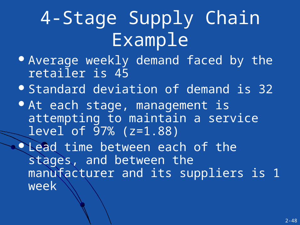
4-Stage Supply Chain Example
Average weekly demand faced by the retailer is 45
Standard deviation of demand is 32 At each stage, management is attempting
to maintain a service level of 97% (z=1.88) Lead time between each of the stages,
and between the manufacturer and its suppliers is 1 week

2-49
Costs and Order Quantities
K D H Q
retailer 250 45 1.2 137
distributor 200 45 .9 141
wholesaler 205 45 .8 152
manufacturer 500 45 .7 255

2-50
Reorder Points at Each Stage
For the retailer, R=1*45+1.88*32*√1 = 105For the distributor, R=2*45+1.88*32*√2 =
175For the wholesaler, R=3*45+1.88*32*√3 =
239For the manufacturer, R=4*45+1.88*32*√4
= 300

2-51
More than One Facility at Each Stage
Follow the same approach Echelon inventory at the warehouse is the
inventory at the warehouse, plus all of the inventory in transit to and in stock at each of the retailers.
Similarly, the echelon inventory position at the warehouse is the echelon inventory at the warehouse, plus those items ordered by the warehouse that have not yet arrived minus all items that are backordered.

2-52
Warehouse Echelon Inventory
FIGURE 2-14: The warehouse echelon inventory

McGraw-Hill/Irwin Copyright © 2008 by The McGraw-Hill Companies, Inc. All rights reserved.
Chapter 5
The Value of Information

2-54
5.1 Introduction
Value of using any type of information technology
Potential availability of more and more information throughout the supply chain
Implications this availability on effective design and management of the integrated supply chain

2-55
Information Types
Inventory levelsOrdersProductionDelivery status

2-56
More Information Helps reduce variability in the supply chain. Helps suppliers make better forecasts,
accounting for promotions and market changes. Enables the coordination of manufacturing and
distribution systems and strategies. Enables retailers to better serve their customers
by offering tools for locating desired items. Enables retailers to react and adapt to supply
problems more rapidly. Enables lead time reductions.

2-57
5.2 Bullwhip Effect
While customer demand for specific products does not vary much
Inventory and back-order levels fluctuate considerably across their supply chain
P&G’s disposable diapers caseSales quite flatDistributor orders fluctuate more than retail
salesSupplier orders fluctuate even more

2-58
4-Stage Supply Chain
FIGURE 5-5: The supply chain
2-59
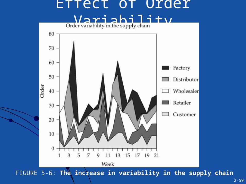
Effect of Order Variability
FIGURE 5-6: The increase in variability in the supply chain

2-60
Factors that Contribute to the Variability - Demand Forecasting
Periodic review policy Characterized by a single parameter, the base-stock
level. Base-stock level =
Average demand during lead time and review period + a multiple of the standard deviation of demand during lead time and review period (safety stock)
Estimation of average demand and demand variability done using standard forecast smoothing techniques.
Estimates get modified as more data becomes available
Safety stock and base-stock level depends on these estimates
Order quantities are changed accordingly increasing variability

2-61
Increase in variability magnified with increasing lead time.
Safety stock and base-stock levels have a lead time component in their estimations.
With longer lead times: a small change in the estimate of demand variability
implies a significant change in safety stock and base-stock
level, which implies significant changes in order quantities leads to an increase in variability
Factors that Contribute to the Variability – Lead Time

2-62
Factors that Contribute to the Variability – Batch Ordering
Retailer uses batch ordering, as with a (Q,R) or a min-max policy
Wholesaler observes a large order, followed by several periods of no orders, followed by another large order, and so on.
Wholesaler sees a distorted and highly variable pattern of orders.
Such pattern is also a result of: Transportation discounts with large orders Periodic sales quotas/incentives

2-63
Factors that Contribute to the Variability – Price Fluctuations
Retailers often attempt to stock up when prices are lower. Accentuated by promotions and discounts at
certain times or for certain quantities. Such Forward Buying results in:
Large order during the discountsRelatively small orders at other time periods

2-64
Factors that Contribute to the Variability – Inflated Orders
Inflated orders during shortage periods Common when retailers and distributors
suspect that a product will be in short supply and therefore anticipate receiving supply proportional to the amount ordered.
After period of shortage, retailer goes back to its standard ordersleads to all kinds of distortions and variations
in demand estimates

2-65
Quantifying the Bullwhip Consider a two-stage supply chain:
Retailer who observes customer demand Retailer places an order to a manufacturer.
Retailer faces a fixed lead time order placed at the end of period t Order received at the start of period t+L.
Retailer follows a simple periodic review policy retailer reviews inventory every period places an order to bring its inventory level up to a
target level. the review period is one

2-66
Quantifying the Bullwhip
Base-Stock Level = L x AVG + z x STD x √LOrder up-to point = If the retailer uses a moving average
technique,
tt LSzL ̂
t
p
Dt
ptii
1
1
)(1 2
2
p
DS
t
pti ti
t

2-67
Quantifying the Increase in Variability
Var(D), variance of the customer demand seen by the retailer
Var(Q), variance of the orders placed by that retailer to the manufacturer
When p is large and L is small, the bullwhip effect is negligible.
Effect is magnified as we increase the lead time and decrease p.
2
2221
)(
)(
p
L
p
L
DVar
QVar

2-68
Lower Bound on the Increase in Variability Given as a Function of p
FIGURE 5-7: A lower bound on the increase in variability given as a f unction of p
2-69
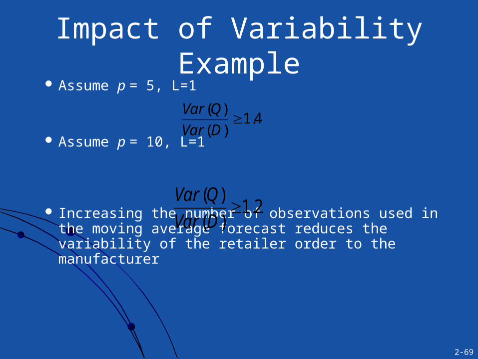
Impact of Variability Example Assume p = 5, L=1
Assume p = 10, L=1
Increasing the number of observations used in the moving average forecast reduces the variability of the retailer order to the manufacturer
4.1)(
)(
DVar
QVar
2.1)(
)(
DVar
QVar

2-70
Impact of Centralized Information on Bullwhip Effect
Centralize demand information within a supply chainProvide each stage of supply chain with
complete information on the actual customer demand
Creates more accurate forecasts rather than orders received from the previous stage

2-71
Variability with Centralized Information
Var(D), variance of the customer demand seen by the retailer
Var(Qk), variance of the orders placed by the kth stage to its
Li, lead time between stage i and stage i + 1
Variance of the orders placed by a given stage of a supply chain is an increasing function of the total lead time between that stage and the retailer
2
2
11)(22
1)(
)(
p
L
p
L
DVar
QVark
i i
k
i ik

2-72
Variability with Decentralized Information
Retailer does not make its forecast information available to the remainder of the supply chain
Other stages have to use the order information
Variance of the orders: becomes larger up the supply chain increases multiplicatively at each stage of the supply
chain.
)22
1()(
)(2
2
1 p
L
p
L
DVar
QVar ik
i
ik

2-73
Managerial Insights
Variance increases up the supply chain in both centralized and decentralized cases
Variance increases:Additively with centralized caseMultiplicatively with decentralized case
Centralizing demand information can significantly reduce the bullwhip effect Although not eliminate it completely!!

2-74
Increase in Variability for Centralized and Decentralized
Systems
FIGURE 5-8: Increase in variability for centralized and decentralized systems
2-75
Methods for Coping with the Bullwhip
Reducing uncertainty. Centralizing information
Reducing variability. Reducing variability inherent in the customer
demand process. “Everyday low pricing” (EDLP) strategy.

2-76
Methods for Coping with the Bullwhip Lead-time reduction
Lead times magnify the increase in variability due to demand forecasting.
Two components of lead times: order lead times [can be reduced through the use of cross-
docking] Information lead times [can be reduced through the use of
electronic data interchange (EDI).]
Strategic partnerships Changing the way information is shared and inventory
is managed Vendor managed inventory (VMI)
Manufacturer manages the inventory of its product at the retailer outlet
VMI the manufacturer does not rely on the orders placed by a retailer, thus avoiding the bullwhip effect entirely.

2-77
5.5 Information for the Coordination of Systems
Many interconnected systems manufacturing, storage, transportation, and retail
systems the outputs from one system within the supply chain
are the inputs to the next system trying to find the best set of trade-offs for any one
stage isn’t sufficient. need to consider the entire system and coordinate
decisions Systems are not coordinated
each facility in the supply chain does what is best for that facility
the result is local optimization.

2-78
Global Optimization
Issues:Who will optimize?How will the savings obtained through the
coordinated strategy be split between the different supply chain facilities?
Methods to address issues:Supply contractsStrategic partnerships

2-79
5.6 Locating Desired Products Meet customer demand from available retailer
inventory What if the item is not in stock at the retailer?
Being able to locate and deliver goods is sometimes as effective as having them in stock
If the item is available at the competitor, then this is a problem

2-80
5.7 Lead-Time Reduction Numerous benefits:
The ability to quickly fill customer orders that can’t be filled from stock.
Reduction in the bullwhip effect. More accurate forecasts due to a decreased forecast horizon. Reduction in finished goods inventory levels
Many firms actively look for suppliers with shorter lead times
Many potential customers consider lead time a very important criterion for vendor selection.
Much of the manufacturing revolution of the past 20 years led to reduced lead times

2-81
5.8 Information and Supply Chain Trade-Offs
Conflicting objectives in the supply chainsDesigning the supply chain with conflicting
goals

2-82
Trade-Offs: Inventory-Lot Size Inventory-Transportation Costs Lead Time-Transportation Costs Product Variety-Inventory Cost-Customer Service

2-83
5.9 Decreasing Marginal Value of Information
Obtaining and sharing information is not free. Many firms are struggling with exactly how to use the data they
collect through loyalty programs, RFID readers, and so on. Cost of exchanging information versus the benefit of doing so.
May not be necessary to exchange all of the available information, or to exchange information continuously.
Decreasing marginal value of additional information In multi-stage decentralized manufacturing supply chains many of
the performance benefits of detailed information sharing can be achieved if only a small amount of information is exchanged between supply chain participants.
Exchanging more detailed information or more frequent information is costly. Understand the costs and benefits of particular pieces of information How often this information is collected How much of this information needs to be stored How much of this information needs to be shared In what form it needs to shared