Women as Agents of Change: Female Incomes and Household Decisions in South India

Nancy Luke and Kaivan Munshi BREAD Working Paper No. 087

October 2004

© Copyright 2004 Nancy Luke and Kaivan Munshi

B R E A D Working Paper

Bureau for Research and Economic Analysis of Development

Women as Agents of Change: Female Incomes and Household Decisions in South India* Nancy Luke and Kaivan Munshi BREAD Working Paper No. 087 October 2004 JEL Codes: D13. J12. J24. O12. Keywords: Education. Marriage. Networks. Caste. Gender. Household decisions. Female income. ABSTRACT This paper exploits a unique setting - tea estates in the South Indian High Range - to provide empirical support for the view that sustained economic empowerment can lead to social and economic change in even the the most disadvantaged sections of society. Female workers earn substantially more than male workers on the tea estates, and these unusual gender patterns have been in place for multiple generations. In addition, low caste and high caste workers have the same incomes and access to the same facilities on the estates. We find that the low castes have higher schooling and are less likely to marry in the traditional fashion than the high castes, reversing the usual pattern that is found in the rest of South India. Our explanation for these striking results is based on the idea that children’s schooling and marriage are part of a complex set of inter-linked choices that the household must make in a traditional network-based economy. Although low castes have the same income as the high castes on the tea estates, they have inferior extended family networks at home in Tamil Nadu. They will consequently shift resources away from the home network to the nuclear family, which explains the caste-gap in the schooling and marriage choices that the workers make for their children. Looking within the household to better understand the determinants of these choices, we find that a relative increase in female income increases children’s schooling and moves the family away from the traditional social patterns, most significantly among the low castes. Low caste women emerge as independent agents of change, shifting their households from the traditional economy into the modern market economy.

Nancy Luke Kaivan Munshi Brown University Brown University and NBER

Email: munshi@brown.edu * This project could not have been completed without the encouragement and support that we received from Homi Khushrookhan. We are grateful to the management, staff, and workers of Tata Tea, Munnar, for their assistance and gracious hospitality during our extended stays in the tea estates. Binitha Thampi supervised the data collection and, together with Leena Abraham, assisted us in the design of the survey. We are grateful to Suma Chitnis, Raquel Fernandez, Jonathan Gruber, Ignacio Palacios-Huerta, Padma Velaskar and especially Andrew Foster for many helpful discussions. Andrew Foster provided us with the numerical solution to the model and Chun-Fang Chiang, Alaka Holla, and Jonathan Stricks provided excellent research assistance. Sarah Williams and Naresh Kumar assisted us with the geo-mapping. Seminar participants at Brown, NYU, and the University of Washington provided useful comments. Research support from the Mellon Foundation at the University of Pennsylvania and the Harry Frank Guggenheim Foundation is gratefully acknowledged. We are responsible for any errors that may remain.

Women as Agents of Change:

Female Incomes and Household Decisions in South India ∗

Nancy Luke† Kaivan Munshi‡

October 2004

Abstract

This paper exploits a unique setting - tea estates in the South Indian High Range - to provide em-pirical support for the view that sustained economic empowerment can lead to social and economicchange in even the the most disadvantaged sections of society. Female workers earn substantiallymore than male workers on the tea estates, and these unusual gender patterns have been in placefor multiple generations. In addition, low caste and high caste workers have the same incomes andaccess to the same facilities on the estates. We find that the low castes have higher schooling andare less likely to marry in the traditional fashion than the high castes, reversing the usual patternthat is found in the rest of South India. Our explanation for these striking results is based on theidea that children’s schooling and marriage are part of a complex set of inter-linked choices that thehousehold must make in a traditional network-based economy. Although low castes have the sameincome as the high castes on the tea estates, they have inferior extended family networks at homein Tamil Nadu. They will consequently shift resources away from the home network to the nuclearfamily, which explains the caste-gap in the schooling and marriage choices that the workers makefor their children. Looking within the household to better understand the determinants of thesechoices, we find that a relative increase in female income increases children’s schooling and movesthe family away from the traditional social patterns, most significantly among the low castes. Lowcaste women emerge as independent agents of change, shifting their households from the traditionaleconomy into the modern market economy.

Keywords. Education. Marriage. Networks. Caste. Gender. Household decisions. Female income.JEL. D13. J12. J24. O12.

∗This project could not have been completed without the encouragement and support that we received from HomiKhushrookhan. We are grateful to the management, staff, and workers of Tata Tea, Munnar, for their assistance andgracious hospitality during our extended stays in the tea estates. Binitha Thampi supervised the data collection and,together with Leena Abraham, assisted us in the design of the survey. We are grateful to Suma Chitnis, Raquel Fernandez,Jonathan Gruber, Ignacio Palacios-Huerta, Padma Velaskar and especially Andrew Foster for many helpful discussions.Andrew Foster provided us with the numerical solution to the model and Chun-Fang Chiang, Alaka Holla, and JonathanStricks provided excellent research assistance. Sarah Williams and Naresh Kumar assisted us with the geo-mapping.Seminar participants at Brown, NYU, and the University of Washington provided useful comments. Research supportfrom the Mellon Foundation at the University of Pennsylvania and the Harry Frank Guggenheim Foundation is gratefullyacknowledged. We are responsible for any errors that may remain.

†Brown University‡Brown University and NBER

1 Introduction

The past decades have witnessed widespread economic and social change in India. The emergence

of the market economy has resulted in the decline of community-based institutions that traditionally

supported economic activity, with accompanying changes in the underlying social structure. Access

to education and new employment opportunities, particularly in the city, has meant that children are

no longer tied to their parents’ occupations. While this process of change goes back to the colonial

period, it has accelerated since independence in 1947, particularly with the economic and financial

liberalization of the 1990s.

The changes that we have described do not, however, apply evenly across India. Hindu society

was historically organized by caste into hereditary occupations, with the lower castes relegated to

menial and ritually polluting tasks. When new opportunities presented themselves under the British,

the upper castes were quick to gain access to education, and with it coveted administrative and

professional jobs, reinforcing existing economic disparities. Social change has varied by caste as well.

To take one example from the region we study in this paper, perhaps the most distinctive feature

of South Indian kinship structure is cross-cousin marriage (Karve 1953, Dumont 1986, Trautman

1981).1 These marriages traditionally supported a primary social network at the level of the extended

family, with overlapping primary networks linking the endogamous sub-caste, or jati. Marriage outside

the jati, with the stigma that accompanies it, continues to be rare. However, cross-cousin marriage

has been rapidly replaced in economically mobile upper-middle castes throughout South India by

“modern” marriages, for money and status rather than for “love of kin” (Kapadia 1995). While these

changes might allow some community members to take advantage of opportunities in the new market

economy, they will inevitably lead to the disintegration of the traditional community networks with

their patterns of informal reciprocity.

Recognizing the historical inequities that have accompanied the caste system, the government of

India subsidizes schooling, reserves seats in institutions of higher education, and sets aside a substantial

fraction of government jobs for the lower castes. While these policies are motivated to some extent by

notions of fairness, there is in addition the presumption that the economic empowerment of previously

disadvantaged groups will lead to positive economic and social change. Unfortunately, a large caste-

gap in wealth and educational attainment continues to persist in both urban and rural India more1The term “cross-cousin” is somewhat of a misnomer since the most preferred match for a girl is the mother’s younger

brother, followed by the mother’s brother’s son and the father’s sister’s son.

1

than 50 years after independence. Why have some castes adapted to the “modern” market economy,

leaving other, typically low, castes behind? One explanation for this persistence is that the government

programs are not substantial enough, or have not been in place long enough, to overcome the pecuniary

disadvantages and the discrimination that the low castes have historically faced. Another explanation

is that there is something inherent in the social structure of the lower castes due to their historical

circumstances that makes them resistant to change.

Which of these explanations is correct has obvious implications for policy. This paper exploits a

unique setting to provide empirical support for the first, by demonstrating that sustained economic

empowerment can lead to economic and social change even in the lowest of the low castes. Moreover,

we will show that low caste women, who are disadvantaged by both caste and gender, can contribute

disproportionately to this change when economic opportunities are made available to them. The

setting for our analysis is the South Indian High Range, a mountainous area straddling the modern

Indian states of Kerala and Tamil Nadu. The High Range was virgin forest until it was acquired by

British planters and converted into tea plantations in the last quarter of the nineteenth century. Since

the plantation land was previously uninhabited, workers were brought to the High Range from the

plains in Tamil Nadu. Today, the workers on the tea plantations - or estates - are the third-generation

descendants of those migrants, whose population is supplemented by a fresh influx of new workers

from the “low country” in each subsequent generation through marriage.

The relatively isolated tea estates are well suited to the analysis we have in mind for two reasons.

First, in contrast with the pattern elsewhere in India, both men and women work on the tea estates.

Women work primarily as tea-leaf pluckers, whereas the men are employed in supporting tasks such as

weeding, spraying, and pruning, as well as in the estate tea factories. The women actually earn 25%

more than the men on average, and these unusual wage patterns have now been in place for multiple

generations.

The second advantage of the setting we have chosen is that jobs are not assigned by caste in the tea

estates, in contrast once again with the patterns elsewhere in India. While the inequities of the caste

system are well known, a particularly egregious feature of this system specific to South India was the

institution of agrestic slavery, which committed the members of certain agricultural labor sub-castes,

or jatis, to a lifetime of servitude. These jatis went by different names in different parts of South India;

in the Tamil country there were two slave jatis, known as the Pallars and the Paraiyars, who together

accounted for somewhere between 10 and 20 percent of the total population in the nineteenth century

2

(Kumar 1965).2 The emancipation of slavery in India in the last quarter of the nineteenth century

coincided with the opening of the tea estates in the High Range, and not surprisingly the bulk of

plantation labor was made up of former slaves looking to improve their opportunities. Two-thirds of

the workers in the High Range today are Pallars and Paraiyars and much of the analysis in this paper

will classify these former slave castes as “low castes,” combining all the other castes in the tea estates

in the “high caste” category. What is remarkable about the plantation system is that the former

slaves, the lowest of the low castes, have the same jobs and access to the same housing, educational,

and medical facilities as the upper caste workers on the tea estates.

The data used in the analysis are obtained from a single firm, the largest tea manufacturing

company in the world, that operates 23 estates in the High Range. Each estate employs approximately

one thousand workers. Annual incomes for all workers were obtained over the 1997-2001 period from

the company’s computerized records. In addition, we surveyed a random sample of 3,700 female

workers drawn from all 23 estates in 2003. The selected female workers were interviewed in their

homes, and detailed information on the background of the respondent, her husband, and their parents

was collected. Information on the schooling and marriage choices that the workers made for their

children was also collected.

The empirical analysis begins by comparing workers by caste. Low and high caste workers have

the same age and income in the tea estates. We mentioned earlier that an important dimension of

social change in South India is the steady decline in cross-cousin marriage, with resulting implications

for the integrity of the traditional caste networks. And education is perhaps the best determinant of

economic mobility in a modern economy. We find that low caste workers are much less likely to marry

a relative in the traditional fashion and that they have significantly higher schooling than the high

caste workers. These marriage and schooling patterns are quite the opposite of what we would expect

to find elsewhere in South India, emphasizing the point that the low castes are at least as responsive

to new opportunities as the high castes once the usual income disparities are controlled for.

Why do the low castes have higher schooling? The explanation for this striking observation that

we put forward in this paper draws on the fact that the workers continue to be tied to their origin

communities in rural Tamil Nadu, despite having lived in the tea estates for many generations. Loans

and reciprocal transfers flow back and forth between the tea estates and the origin location, the

children of the workers are often sent home to study, and many workers will buy land, build a house,2Pallar is derived from pallam, the Tamil word for lowness and Paraiyar means outcaste (hence the English “pariah”).

3

and return to their rural homes when they retire. Most importantly, many workers continue to marry

their children to relatives from the origin location in the traditional fashion. A household in the

tea estates can thus invest its scarce resources in an network located in the origin location, with the

expectation that it will receive a return on that investment in the future. Marrying a child to a

relative strengthens social ties and increases the returns to investment in this network. Alternatively,

the household can invest in its children, particularly in their education, with the expectation that the

parents will be supported by their children in old-age.

Everything else being equal, a household with a weaker home network will distance itself from the

origin location, investing more in the children and being less likely to marry them into the network

(to a relative). A network’s quality will in general depend on the economic circumstances of its

members. Given the persistent caste differences in socioeconomic status outside the tea estates it

seems reasonable to assume that the low caste workers will have access to inferior networks back home

in Tamil Nadu. This explains why low caste workers have more schooling and are less likely to be

married to a relative or someone from their home location. It also explains why the parents of the low

caste workers are less likely to retire in their original homes in Tamil Nadu, presumably because they

have invested less in their (inferior) networks over the course of their working lives.3

When households make choices in a network-based economy, these choices often have long-term

implications. For example, when a child is schooled away from the origin location or married outside

the network, this choice affects the social support that the parents will receive in the future. Stable

economic opportunities over the workers’ lives, and over many generations, undoubtedly played an

important role in allowing households in the tea estates to break away from traditional patterns of

behavior and shift investments away from the network to the nuclear family. The basic tradeoff

between the extended family and the nuclear family has existed in the tea estates for generations,

and not surprisingly the caste differences in schooling and marriage that we described above for the

workers are obtained for their children as well.

Parents make schooling and marriage choices for their children in this society and so we proceed

to look within the household to better understand the determinants of these choices. Female income-

generation programs worldwide are predicated on the assumption that money in the hands of women3Along the same lines, Akresh (2004) shows in an interesting recent paper that network quality affects household

choices in Burkina Faso. The advantage of the research setting that we have chosen is that incomes do not vary by castein the tea estates, while the quality of the networks varies exogenously by caste, allowing us to more cleanly identify therole of community-based networks in shaping household decisions.

4

will be put to different use than money in the hands of men. Consistent with this view, we find that

an exogenous increase in female income, net of total household income, weakens the family’s ties to

the network; the children are less likely to marry a relative, they are less likely to be schooled in the

origin location, and they are less likely to ultimately settle there. At the same time, an exogenous

increase in relative female income increases the educational attainment of the children. While the

female income effects go in the same direction for both castes, they are much larger (and statistically

significant) for the low castes. Low caste women thus appear to contribute disproportionately to the

changing patterns of behavior in their community.

Once again, there is a simple network-based story for the results that we obtain. A female income

effect is indicative of differences in preferences by gender, with a relative increase in female income

moving the household to a point on the Pareto frontier that is preferred by the woman. Selfish

parents making schooling and marriage choices for their children will only consider the returns to their

investment in the network versus investments in the children. In particular, they will not internalize

the potentially substantial pecuniary and non-pecuniary costs to the children when they are married

into the network and end up living and working in the origin location. If we make the assumption

instead that mothers are more altruistic toward their children than fathers, then this implies that the

mothers have a greater incentive than the fathers to move their families away from the home network.4

This wedge between male and female preferences will be greater in the low castes, since their inferior

networks impose a greater cost on the children, allowing us to explain both the direction of the female

income effect as well as the fact that it is stronger among the low castes.

There is a large literature both in economics and sociology that seeks to understand how the

distribution of income within the household affects the allocation of resources (see Behrman 1997 and

Strauss and Thomas 1995 for exhaustive reviews). This literature is largely concerned with the choice

between private goods, which are enjoyed by a single individual, and public goods - notably children

- that benefit multiple individuals in the household. Consequently, much of the previous empirical

work has studied whether and how expenditures on different goods, particularly child education and

nutrition, vary with female income net of total household income. In contrast, we analyze how the

choice between investing in the network and the nuclear family (children’s education) is shaped by the4The mother takes almost complete responsibility for child care in this society and simply by virtue of having spent

more time with the children she might be more attached to them. Cox (2003) offers an alternative explanation fromevolutionary biology, based on paternity uncertainty, as to why mother’s might care more about their children’s welfarethan fathers.

5

distribution of income within the household. This allows us to evaluate the effect of female income on

major decisions such as where to go to school and whom to marry, as well as on long-term outcomes

such as educational attainment and residential location.

In line with the results from the received literature, we find that an increase in female income does

lead to an increase in children’s schooling. But the additional caste dimension that we incorporate in

the analysis tells us that these effects vary by social group and are concentrated among the low castes.

Recent research from Bombay (Munshi and Rosenzweig 2003) shows that girls are more receptive

to new career opportunities, as measured by the schooling choices that are made for them by their

parents, than boys, who tend to be held back by the (male) caste-based labor market networks that

have historically operated in the city. In the tea estates we see once again that the groups with the

inferior (weaker) networks - in this setting, the low castes - are more receptive to new opportunities, as

demonstrated by their schooling and marriage choices. The analysis in Bombay treats the household

as the decisionmaking unit. In the tea estates, we find that female workers emerge as active agents of

change when we look within the household.

The paper is organized in five sections. Section 2 describes the institutional setting, comparing

high and low castes in rural Tamil Nadu, as well as in the estates, by gender. A brief history of

the tea estates is also provided. Section 3 presents a simple model of household decision-making

that highlights the tradeoff between investing in the extended family and the nuclear family, with

implications for marriage and schooling decisions. The model also allows us to explain the female

income effects and the total income effects that we obtain in the empirical analysis. Section 4 presents

the empirical results, beginning with simple caste-wise comparisons of schooling and marriage among

the workers’ children, by gender, and then proceeding to the regressions described above. Alternative

interpretations of the female income effect are also discussed in this section. Section 5 concludes.

2 The Institutional Setting

2.1 Caste and Gender in South India

Hindu society is divided hierarchically into four broad caste categories or varnas: Brahmins, Ksha-

triyas, Vaishyas, and Shudras. Within each varna are myriad endogamous sub-castes or jatis. And

arrayed below the four varnas, outside the caste system proper, are another host of untouchable jatis.

The slave castes occupied positions at the very bottom of this complex social system in South India.

6

The caste system was formerly abolished with independence in 1947, but little has changed for

many of the lowest castes. Kapadia’s study (1995) set in one rural Tamil village, for example, describes

how “the Pallars, Christian Paraiyars, and Wottans (Hindu Paraiyars) in Aruloor all continue to

be regarded as ‘untouchables,’ as they have been for centuries” (p. 9). Recognizing the historical

inequities that accompanied the caste system and the persistence of many of these inequities, the

government of India has taken steps to economically empower the lowest castes by subsidizing their

schooling, reserving seats in institutions of higher education, and setting aside a substantial fraction

of government jobs for them. The former untouchable castes, which include the slave castes, as well as

some Shudras who traditionally performed particularly abhorrent tasks are designated as Scheduled

Castes (SC’s) and deemed eligible for these government programs. Since caste has been officially

abolished, government statistics and large-scale data sets like the National Family Health Survey

(NFHS) classify individuals by their Scheduled Caste status alone. Thus, detailed jati-level data have

been unavailable from official sources since independence, complicating the comparison of outcomes

in the tea estates with outcomes in the workers’ origin locations in rural Tamil Nadu.

Our explanation for cross-caste differences in schooling and marriage in the tea estates is based

on the idea that, while all workers in the estates have access to the same opportunities and services,

conditions vary by caste at home in rural Tamil Nadu. To verify this view of the home communities,

we compare Scheduled Castes (SC’s) with non-Scheduled Castes (non-SC’s) in rural Tamil Nadu, using

the most recent (1999) NFHS. Ideally, we would have liked to compare the slave castes with the castes

above them, but as noted, jati-level statistics are unavailable from standard data sources. The SC

and non-SC comparison nevertheless allows us to verify that the traditional caste hierarchy continues

to affect economic and social outcomes today.

The sampling frame for the NFHS is ever married women aged 15-49. Detailed information is

collected from each selected woman and her spouse (where relevant). Additional information on all

individuals residing in the house is collected in a separate household module. Comparing the SC and

non-SC husbands in rural Tamil Nadu in Table 1, Columns 1-2, there are no caste differences by age,

but schooling is significantly higher among the higher caste men. Employment levels are extremely

high in both caste groups, but non-SC men are much more likely to be employed in skilled occupations.

The NFHS does not report incomes, but these occupational differences indicate that incomes will be

greater in the higher castes. Munshi and Rosenzweig (2003) report the same cross-caste patterns in

Bombay city, with high caste men having more schooling, being more likely to be employed in skilled

7

occupations, and having higher incomes than low caste men. The quality of a caste network in terms

of its ability to smooth risk, provide credit, and generate jobs will, in general, depend on the wealth

of its members. The preceding discussion suggests that high caste networks will be superior to low

caste networks in rural Tamil Nadu, as they are elsewhere in the country.

Comparing SC and non-SC women in Columns 3-4, both age and schooling do not vary by caste.

High caste women traditionally did not enter in the labor market, lowering their returns to schooling

and, by extension, their educational attainment. Consistent with this view, low caste women are much

more likely to be employed than high caste women, although they are less likely to hold a skilled job

conditional on being employed. Participation in the labor force has been seen to result in greater

autonomy for low caste women (Kapadia 1995, Geetha 2002, Chakravarty 1993), and we will return

to this point later in Section 4.4 as an alternative explanation for the differences in the female income

effect by caste.

2.2 A Brief History of the Tea Estates

The South Indian High Range was historically part of the state of Travancore; today it is situated

in the modern Indian state of Kerala (on the border with Tamil Nadu). Travancore was nominally

under the control of a native ruler, but under pressure from the local British Resident and European

entrepreneurs, the government of Travancore began to grant “concession” land in perpetuity for the

cultivation of coffee from the 1860s onward.

After leaf disease destroyed the coffee crop in the 1870s, the British planters experimented with a

number of crops before settling on tea. By the beginning of the twentieth century, the High Range,

also known as the Kannan Devan Hills, had developed into the most important tea producing area

in Travancore. The shift from coffee to tea led to fundamental changes in the operations of the

plantations. Tea plantations require a stable workforce, and while coffee could be simply left to dry in

the sun, the tea leaves had to be processed in a nearby factory before being transported. The original

individual- or family-owned plantations were consequently consolidated over time to take advantage

of economies of scale. In 1890 James Finlay and Company made an offer for the entire Kannan Devan

Hills concession, which was ultimately accepted by the planters in 1897 after lengthy negotiations.

Since the concession land was previously uninhabited, labor had to be imported from elsewhere.

For reasons that are unclear to historians familiar with the area, it proved difficult to recruit labor from

Travancore itself. Instead, the planters brought up workers from the plains in the Madras Presidency

8

(the modern Indian state of Tamil Nadu). As we will discuss below, a large proportion of these workers

belonged to the slave castes. Slavery in India differed from slavery in other parts of the world in two

important respects. First, the slaves in India could only be drawn from specific castes. And, second,

these slaves belonged to the same race and culture as their masters and enjoyed certain rights, such as

a customary wage (Kumar 1965, Alexander 1989). Nevertheless, the slave castes remained the most

wretched and downtrodden groups in South Indian society. Samuel Mateer, a Christian missionary

writing in 1884 (cited in Kooiman 1989: 18), describes how the slaves were “bought and sold like

cattle, flogged like buffaloes, made to work all day for a little rice, and kept at a distance as polluted

... suffering from ignorance and evil habits of drunkenness and vice.”

The British noted the existence of slavery as soon as they arrived in South India at the beginning

of the nineteenth century, but they did little to change the system initially except to protect the slaves

from the worst abuses of the system (Kumar 1965). The anti-slavery movement in Britain ultimately

pressured the Government of India to pass the Slavery Abolition Law, Act V, in 1843. This simply

meant that the administration would no longer apprehend and bring back runaway slaves to their

masters and that no claims to the services of slaves could be upheld in British courts. It was only

with the passing of the Penal Code in 1861 that a man could actually face legal prosecution if found

in the possession of a slave, finally freeing the slave castes (Hjejle 1967).

The emancipation of the slaves coincided with the opening up of the plantations in the High Range,

and not surprisingly a large proportion of the labor force was recruited from the (former) slave castes,

who were looking to improve their economic opportunities. At the same time, upper caste workers are

well represented in the tea estates. Using census data, Kumar (1965) documents that the population

of the Madras Presidency, the major source region for labor in the tea estates, rose by 300 percent

between 1802 and 1901. This population increase, together with the structural change in the economy

brought about by colonialism, displaced many individuals from their traditional caste occupations,

inducing them to migrate to the tea estates as agricultural labor.

Initially the planters sent their own agents to recruit workers from the plains. But within a short

time the workers began to migrate on their own, in gangs drawn from the same jati, and led by

a kangany, or foreman. The kangany was responsible for transporting his gang to the High Range

(a dangerous and arduous journey), negotiating wages and other employment conditions there, and

eventually supervising his workers (Kumar 1965). The size of the workforce fluctuated with the

tea crop in the early years, and workers were recruited on fixed term contracts usually running for

9

nine months (Baak 1997). The problem with the short-term contracts was that the workers would

often return to the plains without advanced notice or be easily induced to switch companies at a

slightly higher wage. The Criminal Breach of Contract Act, introduced in 1865 by the Travancore

government, helped reduced this problem for a while. But the planters were forced to switch to a

permanent workforce with the abolition of the Act in the 1930s. With all the unpredictable movement

back and forth between the High Range and Tamil Nadu, it is unlikely that the workers were sorted

across Finlay estates by ability when permanent employment status was first granted.

Permanent workers and their families were provided free housing in “labor lines” located on each

estate. To ensure that children of the workers would be employed in the future, company rules

prevented workers from shifting across estates, or new workers from entering the estates, except

through marriage. James Finlay and Company gradually sold all its properties to a wholly Indian-

owned company, Tata Tea, over the course of the 1970s and 1980s, and the divestment process was

completed in 1986. Tata Tea has continued to keep the rules restricting worker mobility in place.

The workers on the tea estates are the third generation descendants of the workers who were hired

permanently in the 1930s, supplemented by the influx of fresh migrants in each generation that followed

through marriage. This stability in economic opportunities, over the worker’s lifetime and across

multiple generations, no doubt played an important role in the shift away from home networks that

we document below.

2.3 Caste and Gender in the Tea Estates

This paper uses data collected by the authors in two phases in 2002-2003. Tata Tea owns 23 tea

estates in the High Range, and each estate employs approximately 1000 workers. Annual incomes for

all workers over the 1997-2001 period were obtained from the company’s computerized records on an

initial trip to the tea estates in February-March 2002. Historical rainfall data from 1965 to 2001 and

the elevation of each estate were also collected on this visit. Subsequently, we conducted a survey of

4,000 female workers on a second visit, from December 2002 to March 2003.

Each estate office maintains a “family card” listing the individuals residing in each unit in the

labor lines and their relationship to the (typically male) household head. The information on the

family cards was collected and entered on computer on our first visit to the tea estates in 2002,

and the sampling frame for the subsequent survey in 2002-2003 was restricted to wives of (male)

household heads. The sampling frame ultimately comprised 11,700 women from which 4,600 were

10

drawn randomly and interviewed at their homes.

Since the list of workers was one year old at the time of the survey, some of the workers in the

sample had left employment by February 2003. Other workers were not at home on the day of the

interview and the revisit date. The 4,600 selected workers reside in 86 divisions in the 23 estates

spread all over the area (some of the estates are as far as 25 km from Munnar, the only town in the

area, where the survey team was based). Female workers pluck tea from 8AM until 5PM on weekdays,

so they could only be interviewed in the late evenings and on weekends. These logistical difficulties

forced us to schedule only one call-back for missed interviews. Nevertheless, 3,994 schedules were

ultimately completed, leaving us with an overall response rate of 89.1%. Leaving aside the women in

our sample who had left the company, the response rate increases to 93.4%.

Each worker is assigned a permanent identity number by the company, which we used to merge

the survey data with the individual incomes collected earlier from the company’s records. Discarding

mismatches between the identity numbers recorded in the survey and the administrative records, as

well as mismatches between the identity numbers in the survey and the family card, we were left with

3,700 couples in which the woman was the wife of a household head and for whom we had income

information for both spouses. The survey instrument collected detailed information on the background

of the respondent, her husband, and their parents. We also collected information on the respondent’s

children and their spouses (where relevant), paying particular attention to the marriage and schooling

choices that were made by the workers for their children.

Table 2 begins by comparing age, income, and schooling by caste, separately for male and female

workers. Columns 1-4 use the Scheduled Caste (SC) classification to partition the workers by caste

in a manner that is consistent with the NFHS data presented earlier in Table 1. Low caste and high

caste workers, both males and females, have the same age and income in the tea estates. Comparing

schooling by caste, low caste (SC) men have significantly higher schooling than upper caste (non-SC)

men in the tea estates. The caste-gap goes in the same direction for the women, although the difference

is not significant at the 5 percent level. Columns 5-8 repeat the cross-caste comparison, including only

Pallars and Paraiyars - the former slave castes - in the low caste category. Once again, age and income

are indistinguishable by caste for men and women. But the caste-gap in schooling now widens, and

low caste men and women have significantly higher schooling than the high castes.

The equality of incomes across castes, and the higher schooling among the low castes, contrasts

with the patterns from rural Tamil Nadu reported in Table 1 and, in general, what we would expect to

11

find elsewhere in the country. The higher schooling among the low castes was previously attributed to

their inferior networks at home, which would have lead them to invest in the nuclear family (children’s

education) rather than the extended family.

Despite having been in the High Range for many generations, the workers are still tied to their

communities in the low country. They send their children to study in the low county, the children

settle at home, and, in some cases, the workers buy land and build a house for retirement in the origin

location. The institution most responsible for keeping these ties in place over so many generations is

undoubtedly the marriage institution. Endogamous marriage within the jati has been seen to have

historically kept networks in place, even in the city (Munshi and Rosenzweig 2003). As noted, marriage

in South India traditionally occurred among relatives, with overlapping networks linking the entire

jati. Kapadia’s (1995: 19) ethnographic research in a Tamil village describes how “marriageable kin

(kalyana murai) were more important in everyday life than lineage kin (pankali). The simple fact was

that one got more from them [affines] than from patrilineal [lineage] kin, and for this reason one was

more involved with them.” Those workers in the estates that followed traditional marriage patterns

typically found related spouses who resided in the origin location for their children.5 These marriages

would have strengthened social ties, increasing the returns to investment in the home network.

But marriage patterns respond to changes in the economic environment. Traditional cross-cousin

marriage, for example, has declined all over South India in recent decades, with relatively wealthy

and educated individuals exiting the network to match on the “open” marriage market. In the tea

estates we would expect the low castes to show the greatest propensity to deviate from the traditional

marriage pattern, since incomes in the tea estates do not vary by caste but low caste networks at home

are of relatively poor quality. Table 2, Panel B compares marriage patterns by caste in the tea estates.

To begin with, we see that both low caste and high caste workers adhere to the fundamental social rule

of marriage within the jati. The low castes actually have slightly lower levels of out-marriage, perhaps

due to the continuing stigma associated with marriage into the former slave castes. However, consistent

with the preceding discussion, the low caste workers are much less likely to marry a relative. It then

follows mechanically that the high caste workers will be more likely to be first generation arrivals in

the tea estates. Households that distance themselves from the home community invest less in the5Traditionally the most preferred matches for a woman are the mother’s brother, the mother’s brother’s son, and the

father’s sister’s son. Among our female respondents who married a relative, 12.5% married the mother’s brother, 25.4%married the mother’s brother’s son, and 22.3% married the father’s sister’s son. The remaining 39.8% married someother relative.

12

extended family network, allocating resources instead to educating their children and making other

investments in the nuclear family. Not surprisingly, the parents of the low caste workers are much less

likely to have retired in the home location. This tradeoff between the extended family and the nuclear

family also explains the higher schooling among the low castes in the tea estates reported earlier in

Table 2, Panel A.

The descriptive statistics reported this far have used two alternative caste classifications to par-

tition the sample. While the results are for the most part robust to the classification scheme, the

historical background presented earlier suggests that the classification restricting the low castes to the

former slave castes, the Pallars and the Paraiyars, may be more appropriate. The slave castes faced

particularly adverse circumstances, and the emancipation of slavery by the British and the abolition

of the caste system by the Indian government have failed to substantially change the economic and

social circumstances of these lowest of the low castes.

One concern with this alternative classification is that we end up comparing the lowest castes with

those just above them, since some of our designated high castes will now be Schedule Castes. Four

jatis - Pallars, Paraiyars, Sakliars, and Thevars - account for 87% of our sample. While the Sakliars

are also classified as Scheduled Castes, the Thevars are a “forward” or high caste. Table 3 compares

marriage patterns and schooling levels among the workers separately for these four jatis. The Pallars

and the Paraiyars look similar on most dimensions that we report. The Sakliars look very different

from the slave castes, emphasizing the diversity that exists within the Scheduled Castes. Indeed,

marriage and schooling among the Sakliars is very similar to the upper caste Thevars. The analysis

that follows will consequently restrict the low castes to the Pallars and the Paraiyars, collecting all

other jatis in the estates in the high caste category. We note that all the results that we subsequently

report would follow through with the alternative SC classification, since the Pallars and the Paraiyars

account for the bulk of the Scheduled Castes in the tea estates.

We close this section by discussing alternative explanations for the caste-gap in schooling and

marriage observed in Tables 2-3. Low caste jatis are larger on average than high caste jatis in the

tea estates as a consequence of historical settlement patterns. Since the social rule of endogamous

marriage within the jati continues to be adhered to, low caste workers will have more eligible partners

who do not belong to their primary extended family network to choose from within the tea estates.

Differences in the local marriage market might then explain differences in marriage patterns and, by

extension, schooling choice across castes. While there are only two low caste jatis, there is sufficient

13

size variation across the more numerous high caste jatis to test whether size affects schooling and

marriage within that broad caste group. Controlling for the age of the man and the woman, we find

that jati size has no effect on these outcomes (not shown).

A second concern is that if workers systematically selected into the tea estates, and these historical

selection pressures varied by caste, then low caste and high caste workers would differ on dimensions

other than network quality, such as individual ability. One simple test of such ability differences would

be to compare incomes in the tea estates by caste. We have already seen that these incomes do not vary

by caste, for both men and women, which indicates that low caste and high caste workers do not differ

with regard to those attributes that determine income in the tea estates. But other attributes, such

as initiative and opportunism, which are not reflected in estate incomes, might nevertheless determine

schooling and marriage choices and, more generally, the response to new opportunities.

We mentioned above that the early migrants faced a long and dangerous journey to the High

Range and extremely inhospitable conditions in the tea estates once they arrived there. The new

economic opportunities came with considerable risk, and only the most adventurous individuals would

have found it worthwhile to migrate. Assuming that high castes had superior opportunities at home

but that opportunities did not vary by caste in the tea estates, just as they do today, only the most

adventurous and opportunistic high castes would have migrated. The selection rule we have just

described explains the higher prevalence of low caste workers in the tea estates, both historically and

today. It also implies that selected entry into the tea estates would have favored the high castes,

at least with regard to those dimensions of ability that affect the cost of migrating to a new and

risky environment.6 Much of the analysis that follows will in any case look within castes to provide

additional support for the view that the tradeoff between the nuclear family and the extended family

is driving household choices in this setting.

3 Household Decisions in a Network-Based Economy

The model laid out in this section describes how households make decisions in a network-based econ-

omy. Low caste networks at the origin are assumed to be inferior to high caste networks. This

assumption, together with the equality of income in the tea estates, allows us to explain the caste dif-6If we allowed for heterogeneous extended family networks within broad caste groups then we would expect high

castes with relatively poor networks to have migrated to the tea estates. But this would, if anything, reduce networkquality differences between low and high castes, providing us with a lower bound on the caste effects that we attempt toidentify in this paper.

14

ferences in schooling and marriage among the workers observed in Tables 2-3. Parents make schooling

and marriage decisions for their children in this society, and we would expect broad caste differences in

network quality to have remained across generations, so our network-based model can be extended to

generate predictions for the choices that the workers make for their children. The effect of household

income, and an independent effect of female income, on schooling and marriage choices within each

caste is consequently derived.

3.1 Timing of Decisions and Returns to Investment

Each individual lives for three periods in the simple overlapping generations model that we present

in this section. The individual is sent to school in the first period; we ignore the temporal aspect of

schooling and assume that educational attainment is determined in the first period itself and depends

on the resources that the parents allocate to schooling. The individual works during the second period

of his life, receiving his income in advance at the beginning of that period. The individual’s parents

arrange his marriage at the beginning of the second period as well, at which time a child is born.

The individual and his spouse use the incomes that they exogenously receive at the beginning of

the second period of their lives to invest in their network at the origin location, invest in their child’s

schooling, and to send transfers to their parents. They will subsequently choose a marriage partner

for their child at the beginning of the third and final period of their lives, in which they will live off

the returns to the investments in the extended family and the nuclear family that they made in the

previous period. Notice that the model ignores ability, which could determine parental incomes as

well as the choices that are made for the children. Unobserved ability will, however, play an important

role in the discussion on identification that follows in Section 4.2.

The returns to the investments that the parents make will depend on the quality of their home

networks, which varies by caste, as well as on the marriage choice that they make for their child.

Cross-cousin marriage, typical of the South Indian kinship system, strengthens existing network ties

instead of building new ones, as in North India. South Indian kin networks have thus been seen to be

more cohesive, albeit restricted in geographic and social range, than their North Indian counterparts

(Karve 1953, Dumont 1986, Trautman 1981). One way in which workers far away in the tea estates

can compensate for the geographical separation from their community is to marry their child into the

network. Such alliances reduce social distance and lower the probability that members of the network

far away in the origin location will renege on their obligations to the parents in the future. The model

15

thus assumes that the returns to investing in the extended family are higher when the parents marry

their child to a relative, within any caste.

In contrast, we expect that the returns to investment in the child’s schooling will decline with

marriage into the network within any caste. Such marriages increase the probability that the child

will end up living and working in the origin location in rural Tamil Nadu where the returns to schooling

are relatively low. Moreover, individuals that marry on the “open” market match on attributes, such as

education and wealth. Thus, individuals that marry into the network, where matches are determined

by kinship rather than by individual attributes, forego the additional returns to schooling that they

would obtain through the marriage market.

How do the returns to investment in the extended family network and the nuclear family vary

by caste? The low castes were historically relegated to low-paying, menial occupations, and the

persistence of these economic disparities has been noted earlier in the paper. The quality of a network

will depend to a large extent on the resources of its members, so we would expect the quality of the low

caste networks to be relatively poor in this case. This implies, in turn, that the returns to investment

in the network should be lower among the low castes than the high castes.

It is less easy to predict how the returns to schooling vary by caste. Educated children could find

jobs in the city, where the returns to schooling are largely independent of caste.7 But those children

that marry into the network could end up living in the origin location and working in the traditional

caste occupation, in which case the returns to schooling could vary by caste. Schooling is in general a

way to escape the network and the traditional caste occupation. The caste differences in the returns

to schooling that we have described are consequently likely to be small, relative to the corresponding

caste differences in the returns to investment in the extended family network. The model that follows

will assume, for simplicity, that returns to schooling do not vary by caste. Castes will be distinguished

by the returns to investment in the network alone.

3.2 Household Choices (Common Preferences)

Following the set up described above, the parents in household i allocate their second-period income

Ii to schooling their child Si and investment in the network Ki, subject to the budget constraint

Ii = Ki + pSi, where p is the cost of an additional unit of schooling. Notice that we have ignored the7Munshi and Rosenzweig (2003) describe how caste-based networks operate in the city as well. But these networks

tend to be active in jatis that are well established in particular urban centers. None of the jatis in our sample haveestablished such a presence in Indian cities.

16

transfers that the parents must make to the preceding generation, which will depend on the schooling

and marriage choices that were made for them. Household consumption in the second period is also

ignored to simplify the exposition.

The parents make investment decisions at the beginning of the second period of their lives, based

on the returns they expect will accrue to them at the beginning of the next period. We assume for the

present that the preferences of the father and the mother are perfectly aligned, so household income

Ii can be pooled and the household can be treated as the decision-making unit.

Let αIg(Ki), αOg(Ki) represent the payoff from investing Ki in the network when the child subse-

quently marries inside (I) and outside (O) the network, respectively. Following the discussion above,

the returns to investing in the network are higher when the child marries inside the network, αI > αO.

Similarly, let βIh(Si), βOh(Si) represent the payoff from investing Si in schooling, when the child

marries inside and outside the network respectively. Following the previous discussion, βI < βO. We

assume in addition that both the g and the h function are strictly concave, g′(Ki) > 0, g′′(Ki) < 0,

h′(Si) > 0, h′′(Si) < 0, to emphasize the results that we present below.

The parents do not know whether the child will marry inside or outside the network when they

choose Si and, hence, Ki = Ii − pSi, at the beginning of the second period. The marriage choice that

they later make for their child at the beginning of the third period depends on the payoffs in each

marriage state at that time: V Ii ≡ αIg(Ki)+βIh(Si)+εI

i , V Oi ≡ αOg(Ki)+βOh(Si)+εO

i , where εIi , εO

i

are stochastic terms that represent fluctuations in the marriage market, perhaps associated with the

supply of eligible males and females. The parents will choose to marry their child inside the network

if V Ii > V O

i . They will marry their child on the open market if V Ii < V O

i .

Taking income Ii as given, the risk-neutral household chooses Si to maximize the expected payoff

from its investments,

Pr(V Ii > V O

i )[αIg(Ki)+βIh(Si)+E(εIi | V I

i > V Oi )]+Pr(V I

i < V Oi )[αOg(Ki)+βOh(Si)+E(εO

i | V Ii < V O

i )].

The choices that parents make do not affect the returns to investment in any given marriage state

(αI , αO, βI , βO) or the future shocks to the marriage market (εIi , εO

i ). However, these choices do

affect the marriage state that the child ends up in, which will in turn determine the family’s expected

payoff. This feature of the choice problem distinguishes our model from the standard household budget

allocation problem, generating some predictions that we will later argue are specific to economic

environments in which networks are active.

17

The expression for the household’s expected payoff, described above, can be simplified as,

F (∆V )[∆V + ξIi (∆V ) − ξO

i (∆V )] + [ξOi (∆V ) + αOg(Ki) + βOh(Si)]

where ∆V ≡ ∆αg(Ki)+∆βh(Si) measures the additional deterministic return from marrying inside

the network, and F characterizes the distribution of εOi −εI

i . ∆α ≡ alphaI−αO > 0, ∆β ≡ βI−βO < 0.

Notice that F (∆V ) ≡ Pr(V Ii > V O

i ), ξIi (∆V ) ≡ E(εI

i | V Ii > V O

i ), ξOi (∆V ) ≡ E(εO

i | V Ii < V O

i ), can

all be expressed as functions of ∆V .

The second term in square brackets in the expression above represents the expected payoff when the

child marries outside the network. The first term in square brackets reflects the additional (expected)

payoff when the child marries inside the network, which could be negative. Changes in Si affect

the expected payoff when the child marries outside, the additional expected payoff when the child

marries inside, as well as the probability that the child will end up marrying inside, F (∆V ). All the

terms which are functions of ∆V in the expression above distinguish our problem from the standard

household budget allocation decision in which there is only a single state of the world. Collecting all

these terms, W (∆V ) ≡ F (∆V )[∆V + ξIi (∆V ) − ξO

i (∆V )] + ξOi (∆V ), the expression for the expected

payoff can be simplified even further as,

W (∆V ) + αOg(Ki) + βOh(Si).

Maximizing the expected payoff with respect to Si, the first order condition is obtained as

∂W

∂Si+ βOh′(Si) − αOpg′(Ki) = 0. (1)

Assuming that an interior solution to the household’s choice problem is obtained, how do these

choices vary by caste? ∆α, which measures the decline in the returns to investment in the network

when the child marries outside the network, will depend in general on cohesiveness within the caste

and, hence, the propensity of network members to renege on their obligations. While we do expect

that the returns to investment in the network to be lower among the low castes in both marriage

states, we have no prior belief about the cohesiveness of these castes. Thus, we assume that ∆α does

not vary by caste, but that αI , αO are both lower in the low castes. Moreover, we noted earlier that

the returns to schooling should be comparable across castes when the children marry inside or outside

the network. This implies that ∆β, βO do not vary by caste.

18

To derive comparative statics with respect to αO, it is convenient to assume that there is a

continuum of castes indexed by the parameter αO, which is increasing in network quality, and then

implicitly differentiate the first order condition to obtain

dSi

dαO=

pg′(Ki)SOC

.

Since SOC < 0 by assumption, dSi/dαO < 0. Incomes do not vary by caste in the tea estates,

and so the comparative statics derived above imply that the low castes, with lower αO than the high

castes, will invest more in schooling and less in the network than the high castes. What does this tell

us, in turn, about marriage patterns by caste?

d∆V

dαO= [∆βh′(Si) − ∆α · pg′(Ki)]

dSi

dαO> 0

since dSi/dαO < 0. The probability of marrying inside the network F (∆V ) is increasing in ∆V ,

which implies that the low castes, with low αO and hence low ∆V , should be less likely to marry

within their networks. The assumption that low caste workers have access to inferior home networks,

together with the equality of incomes in the tea estates, thus provides a simple explanation for the

caste differences in schooling and marriage among the workers that we noted in Tables 2-3.

3.3 Household Choices (Gender-specific Preferences)

The discussion this far has treated the household as the decision-making unit. We now proceed to

look within the household to investigate whether women emerge as independent agents of change in

this economy using their incomes (net of total household income) to increase investments in children’s

education and to break away from their home networks. When the parents make schooling and

marriage choices for their child above, they only consider the returns to schooling that accrue to

them and, similarly, the benefit they derive from marrying the child inside or outside the network. In

particular, they do not consider the possibly substantial cost to the child from marrying inside the

network and ending up living and working in the origin location. If we make the assumption instead

that the mother cares more for her child than the father and so internalizes these child-specific costs,

then the mother and the father will have different preferences for the child’s schooling and marriage.

When male and female preferences differ within the household, models of collective decision-making

predict that a relative increase in female income will shift household choices along the Pareto frontier

to a point that the woman prefers. This result is obtained regardless of whether additional restrictions

19

are placed on the cooperative equilibrium as in Manser and Brown (1980), McElroy and Horney (1981),

and Lundberg and Pollak (1993), or whether only Pareto optimality is assumed as in Chiappori (1992)

and Browning et al. (1994). To explore an independent role for women in influencing household

decision-making, we consequently estimate regressions of the form

yi = γFIi + λIi + Xiη + εi, (2)

where yi is the choice that household i makes for its child, Ii is total income in the household, FIi

is female income, Xi is a vector of control variables, and εi collects all the unobserved determinants

of the household’s choice. Outcomes of interest yi include schooling attainment, which will depend

on investments in schooling Si, as well as the probability that the child will marry into the network

F (∆V ). We will see that the model generates predictions for the total income effect λ and the

female income effect γ that provide additional support for the view that conditions at the origin shape

household choices in the tea estates.

Begin with the λ coefficient in equation (2). The regressions will be estimated separately by

caste, and so we assume that αO, βO, ∆α, ∆β are constant across households and then proceed to

derive comparative statics with respect to Ii: dSi/dIi and dF (∆V )/dIi. Starting with the effect of

household income on the child’s schooling, the usual result is that an increase in income should increase

investment in schooling (S) and the network (K), since both the g and the h functions are strictly

concave. The complication that arises in this framework is that an increase in income, by changing S

and K, will change the probability that that child will be married into the network. If this probably

increases sufficiently, with its associated decline in the returns to schooling, then the net effect on

schooling could actually be negative.

To illustrate the possibility that an increase in household income could lead to a decline in schooling

when networks are active we solved the model numerically, assuming that εIi , εO

i are characterized by

the extreme value distribution and suitably parameterizing the g(Ki) and h(Si) functions.8 Figure

1 plots the second order condition (SOC) and dSi/dIi for different values of α0. We see that an

interior solution (SOC < 0) is obtained for all values of αO, but that the sign of dSi/dIi is ambiguous,

consistent with the discussion above.8g(Ki), h(Si) are specified to be quadratic functions of Ki and Si respectively (the parameter values used to obtain

the numerical solutions are available from the authors). The advantage of the extreme value distribution is that thefirst order condition has a simple closed form, allowing us to easily compute dSi/dIi, SOC, ∂W/∂Si, and ∂2W/∂S2

i

numerically.

20

To better understand the source of this ambiguity, we implicitly differentiate the first order con-

dition, equation (1), with respect to Ii, noting that ∂W/∂Si = W ′(∆V ) [∆βh′(Si) − ∆αpg′(Ki)], to

obtain

dSi

dIi=

−W ′′(∆V )∆αg′(Ki)∂∆V∂Si

+ p[W ′(∆V )∆α + αO]g′′(Ki)SOC

, (3)

with the second-order condition (SOC) defined by the expression

SOC ≡ ∂2W

∂S2i

+ βOh′′(Si) + αOp2g′′(Ki).

Now consider the situation described in Figure 2, with the same set of parameters as in Figure 1:

∂W

∂Si= W ′(∆V )

∂∆V

∂Si< 0,

∂2W

∂S2i

= W ′′(∆V )(

∂∆V

∂Si

)2

+ W ′(∆V )∂2∆V

∂S2i

> 0.

We noted earlier that ∂∆V/∂Si ≡ ∆βh′(Si) − ∆αpg′(Ki) < 0, and so ∂W/∂Si < 0 implies

W ′(∆V ) > 0. It follows immediately that dSi/dIi > 0 if the first term in the numerator of equation

(3) is ignored. The complication that arises is that W ′′(∆V ) is likely to be positive when ∂2W/∂S2i > 0,

as in Figure 2.9 If W ′′(∆V ) is sufficiently large and positive, then schooling could actually decline in

income, dSi/dIi < 0, from equation (3) above.

For small W ′′(∆V ), the standard result that schooling is increasing in household income will be

obtained. For intermediate (and positive) values of W ′′(∆V ) the comparative statics will be reversed,

but an interior solution (with SOC < 0) continues to be obtained; this is the situation described for

small values of αO in Figure 1. Finally, for large values of W ′′(∆V ), and hence ∂2W/∂S2i , an interior

solution might no longer be obtained (SOC > 0). The assumed concavity in the g and h functions

implies that the returns to S and K will be declining at the margin in any given marriage state. But

the effect of a change in S (and K) on the probability of marrying inside the network is not necessarily

declining in this manner, which is why a corner solution could in principle be obtained.

The regressions that we will later report show that dSi/dIi < 0. Our earlier discussion indicated

that an increase in the probability of marrying into the network with income dF (∆V )/dIi > 0 was a

necessary condition to obtain this result. To verify that this is indeed the case, we proceed to show

that dSi/dIi < 0 implies dF (∆V )/dIi > 0. Differentiating ∆V with respect to Ii,9For ∂2∆V/∂S2

i = ∆βh′′(Si) + ∆αp2g′′(Ki) < 0, W ′′(∆V ) > 0 is a necessary condition for ∂2W/∂S2i > 0, for

∂2∆V/∂S2i > 0 it is a sufficient condition.

21

d∆V

dIi= ∆αg′(Ki) +

∂∆V

∂Si

dSi

dIi.

Since F (∆V ) is increasing in ∆V , the result follows directly from the expression above. The

negative effect of household income on schooling that we later obtain is explained by the fact that an

increase in income ties the household more closely to its network in this economy, lowering the returns

to children’s schooling, and we will verify that an increase in household income indeed increases the

probability that the children will marry within the network.

This last result is very likely to be a consequence of the special economic circumstances in the tea

estates. In most other settings that we would expect to encounter it would be the high income (or high

ability) individuals who would show the greatest propensity to distance themselves from the network,

to avoid subsidizing the other members of the network, and this is what we have found in our own

previous research in Kenya (Luke and Munshi 2003) and India (Munshi and Rosenzweig 2003). The

richer households in this setting might, however, be able to avoid many of their social obligations due

to their geographical separation from their home locations and the relative isolation of the tea estates,

and we will return to this point below.

Next, consider the γ coefficient in equation (2); conditional on household income Ii, what effect

does female income FIi have on household decisions? We mentioned earlier that selfish parents care

only about the returns that they receive from investments in the network and the child. In particular,

they do not internalize the cost to the child from marrying into the network and subsequently living

and working in the origin location. Apart from transfers to the parents, which we can think of as a

“parental tax,” the child must also make transfers to the extended family network. Workers in the

tea estates are relatively wealthy compared with the members of their networks at home. Thus, both

the parents and the child would in general end up subsidizing the other members of the network. We

noted above that geographical distance allows the parents to avoid this subsidy to some extent. But

the “social tax” imposed by the network on a child residing in the origin location could be substantial,

and the altruistic mother making choices for her child will take account of these costs.

Poverty is often associated with negative outcomes such as male alcohol abuse and domestic vio-

lence. For example, high levels of alcohol consumption in the slave castes have been documented as

far back as the nineteenth century (Kooiman 1989). More recently, Kapadia’s (1995: 56) ethnography

of a Tamil village notes that “Pallar women often spoke of the problems caused by excessive male

22

drinking ... violence against women was a visible phenomenon on the Pallar street.” Consistent with

this view, 51% of the low caste female respondents in the NFHS, versus 35% of the high castes, report

having ever been beaten by their husbands. The NFHS also collects information on the number of

individuals in the household who regularly drink alcohol.10 Restricting attention to married men aged

21-65 who are regular residents in the sampled households, 44% of the low caste men versus 27%

of the high caste men regularly drink alcohol (both marital violence and alcohol consumption vary

significantly by caste at the 5 percent level).

A low caste child marrying into the network is unlikely to escape the alcohol abuse and domestic

violence in the origin location. Men do not drink at home and alcohol consumption is typically an

activity shared by men of the same social group; Rao’s (1997) study in rural Karnataka, for example,

describes how drunk men roamed the streets of the village in groups in the late evenings. A low

caste boy who ends up living in the home community will find it difficult to avoid these behaviors,

regardless of his upbringing, and the altruistic mother making choices for her son will take account

of the accompanying social cost. There is a social aspect to marital violence in this society as well,

to the extent that it is perceived to be justified when women fail to conform to traditional roles (Rao

1997, Bugsby 1999; for Bangladesh, see Schuler et al. 1996). A low caste girl sent to marry in the

origin location will face high levels of marital violence, which the altruistic mother might also seek to

avoid.

A mother who takes account of the pecuniary and non-pecuniary costs to the child from marriage

into the network will prefer to shift household investments away from the network relative to her

husband. In terms of the model, this implies that the returns to investment in the network, αI , αO,

are effectively smaller for the woman than her husband. We have already shown that a decline in αO

(and αI), for a given level of household income, leads to an increase in schooling and a decline in the

probability that the child will marry into the network. Conditional on household income, an increase

in female income should have the same effect on household decisions within castes.

The wedge between the selfish father’s preferences and the altruistic mother’s preferences depends

on the costs imposed on the child by marriage into the network. Incomes do not vary by caste in the

tea estates and so the income that the child carries to the network is unlikely to vary appreciably by

caste as well. However, wealth in the network at home will certainly be increasing in caste status,10When men drink in this society, they typically drink to the point of being inebriated (Rao 1997). Thus a man who

drinks alcohol “regularly” is likely to have an alcohol problem.

23

which implies that low caste children marrying into the extended family network will be taxed more

heavily than high caste children. The social problems of alcohol abuse and domestic violence will

also be more acute among the low castes, as discussed above. The gap between the father’s and the

mother’s preferences will consequently be larger among the low castes, which implies in turn that the

female income effect should be larger for the low castes.11

4 Empirical Analysis

The model laid out in Section 3 allows us to interpret the effect of total household income on the

choices that parents make for their children within castes. The model also predicts that a relative

increase in female income, particularly among the low castes, should shift household choices away from

the extended family network. Section 4.1 begins the empirical analysis by comparing child schooling,

marriage, and residence choices by gender and caste. Section 4.2 describes the specification of the

marriage, schooling, and residence regressions. The instrumental variable procedure used to identify

the female and total household income effects is also described in this section. Subsequently, Section

4.3 presents the main empirical results and Section 4.4 completes the empirical analysis by considering

alternative interpretations of the female income effect that we obtain.

4.1 Caste Comparisons for the Children

The differences by caste in the tea estates reported in Tables 2-3 were explained by differences in the

quality of the home network in Section 3. These quality differentials have been in place for generations

and are likely to persist in the future, so we would expect to find a caste-gap in the marriage and

schooling choices that the workers make for their children as well.

There is little variation in the age at entry into the marriage market in this society, and so the

marriage statistics and the marriage regressions that follow restrict the sample to married children

aged 16-45. Table 4, Panel A, describes the marriage choices that the workers make for their children

by caste.12 Most of the children continue to marry within their jati, although a comparison with the

parents in Table 2 indicates that the prevalence of out-marriage has increased over the generations.11The model does not place similar restrictions by caste on the total income effect. There is no apparent relationship

between caste status αO and dSi/dIi, for the parameter space in which dSi/dIi is negative, in the numerical solutionreported in Figure 1. The regression results reported later similarly reveal no relationship between the total incomecoefficient and caste.

1289.5% of the respondents in the survey reported that their marriage was “arranged” by their parents. These numbershave remained very stable over time; 88.7% of their children’s marriages were also arranged.

24

Low caste boys and girls are much less likely to marry a relative, and by extension someone who grew

up in the origin location, than high caste boys and girls. The low castes continue to be less likely to

marry outside their jati, so their greater propensity to marry outside the network cannot be attributed

to increased out-marriage.

Although primary education is available free of cost in the estate school, the parents must pay for

secondary school from the fifth grade (age 10) onward. A number of educational options are available

to the parents. They could send the child to one of the secondary schools in the tea estates or Munnar,

the main town, but these local schools are perceived to be of relatively poor quality. Alternatively,

they could send their child to a school in rural Tamil Nadu and bear the additional monetary cost

of food and accommodation. An intermediate solution is to send the child to school in the parents’

origin location. Schooling choices are limited in that case, but the child can stay with relatives,

reducing the current pecuniary cost to the parents while at the same time increasing future social

obligations. Sending the child to study in the origin location strengthens both the family’s ties and

the child’s ties to the home community, which is presumably what low caste parents want to avoid.

As an additional measure of the family’s ties to the network, we construct a binary location variable

that indicates whether the child was sent to secondary school in the origin location or elsewhere.

Restricting the sample to children currently aged 10-45, low caste children are significantly less likely

to attend secondary school in the origin location in Table 4, Panel B, as expected.

Very few children report more than 11 years of schooling, at which stage the child will be 16

years old. The educational attainment statistics consequently restrict the sample to children currently

aged 16-45, recognizing that final educational attainment will be truncated for some of the youngest

children. The descriptive statistics in Table 2, Panel A and Table 4, Panel B indicate that educational

attainment has increased substantially over the last two generations for both boys and girls. While the

caste-gap that we observed for the mothers in Table 2 persists for the daughters in Table 4, educational

attainment for low caste and high caste boys is statistically indistinguishable. Later we will see that a

relative increase in female income has a much stronger effect on girl’s schooling than boy’s schooling

among the low castes. This shift in household resources toward the girls might explain the relatively

narrow gender-gap in schooling in those castes.

The schooling and marriage choices that parents make for their children will determine where they

will end up living. Low caste children have higher schooling and are less likely to marry a relative than

high caste children. Restricting the sample to children aged 16-45 who have left their parents’ home

25

we see in Table 4, Panel C that low caste children are less likely to reside in the origin location as well.

Looking at these residential choices in more detail, a roughly equal proportion of the low caste and the

high caste boys remain in the tea estates. Among those that leave, however, a substantially greater

proportion of the high caste boys end up in the origin location. For the girls, the big difference between

the castes is that the low caste girls are much more likely to remain on the tea estates, whereas the

high caste girls are much more likely to settle in the origin location.

Table 4, Panel D describes labor market outcomes for the children in Panel C. Employment levels

are roughly the same, by caste, for the boys. Low caste girls, however, are significantly more likely to

be employed than high caste girls. Conditional on being employed, just about a quarter of the boys

work in the tea estates, as compared with three-quarters of the girls. Differences in employment levels

for the girls appear to be driven almost entirely by differences in their residential choices. Finally,

among the boys that work outside the tea estates, a much greater fraction of the low caste boys

are employed in skilled occupations. We noted above that educational attainment does not vary by

caste among the boys. These differences in the type of occupation appear to be a consequence of the

differences in residential location, conditional on having left the tea estates, that we noted in Panel C.

Jobs in the origin location must on average be less skilled than jobs elsewhere to explain the patterns

in Panel D, consistent with our modelling assumption that the returns to schooling are lower inside

the network.

Employment levels are quite low for the girls and among those that work, most find employment

on the tea estates. For the few girls that do work outside the tea estates, the proportions that find

skilled jobs are fairly high and do not vary by caste. The labor market returns to schooling within

the tea estates are low and so the benefit from the higher educational attainment seems to be to allow

the low caste girls to match with better educated boys on the tea estates, keeping them away from

the extended family network in the origin location. Looking back at residential choices in Panel C,

it is worth noting that the caste-gap in the proportion of children residing in the origin location is

greater for the girls than for the boys. Later we will see that the estimated female income effect on

both educational attainment and residential choice is greater for the low caste girls than for the low

caste boys, matching the patterns by caste and gender in Table 4.

26

4.2 Specification and Identification

Next, we look within the caste to better understand how marriage and schooling choices are made.

As discussed in Section 3.3, we will estimate regressions of the form

yij = γFIi + λIi + Xijη + εij , (4)

separately for low castes and high castes. yij is one of the choices that household i makes for child

j, FIi is female income in household i, and Ii is total income (male plus female) in that household.

Xij includes a vector of control variables, such as the child’s cohort, the schooling of each parent,

and whether the parent is a first generation arrival in the tea estates. The child’s cohort controls for

secular changes in economic opportunities, which would have affected schooling and marriage choices

at the time they were made. The parental characteristics control for their preferences for schooling

and ties to the network, which would directly determine the choices they make for their children.

Since many of the workers’ families have been on the same estate for many generations, differences in

household decisions across estates could reflect the cumulative effect of differences in income over many

generations. By including parents’ schooling and marriage (migration) patterns, we isolate the effect

of current generation income on the choices that are made for the children. Overlapping extended

family networks ultimately link all members of the endogamous jati. The results on the income effects

in Section 3.3 were derived for a given network quality, and so we include jati fixed effects in all the

regressions that follow to estimate the income effects within each jati.

Notice that equation (4) has the same specification as the household choice equation (2) described

in Section 3, except that we now allow each household to have multiple children. The model focussed

on investment in schooling and marriage out of the extended family network as the outcomes of

interest. For the empirical analysis, marriage out of the network will be measured by a binary variable

that indicates whether the child marries a relative or not. While investment in schooling is not

observed directly, such investments translate into higher school attainment. We will thus treat years

of completed schooling as the measure of investment in schooling in the empirical analysis, while

allowing for the possibility that this measure could depend, in part, on the child’s unobserved ability.

As noted above, we also use the secondary school location to measure the family’s ties to the

network. In the usual situation where higher income relaxed the household’s liquidity constraint and

at the same time moved it away from the network, we would expect an increase in household income

27

to expand schooling choices outside the tea estates and reduce the probability of sending the child to

school in the origin location. Given the special circumstances in the tea estates, however, with higher

income bringing the household closer to the network, we might expect higher household income to

increase the probability that the child will be sent to school in the origin location. Conditional on

total income, an increase in female income will shift the location choice in the opposite direction, since

the woman wants to distance the family from the network.

The final outcome that we consider is the child’s residential location - a binary variable indicating

whether the child currently resides in the origin location or elsewhere - conditional on having left the

parental home. In general, the location that the child settles in will depend on whom the child married,

where the child was schooled, and the level of educational attainment. If an increase in household

income leads to marriage and schooling choices that bring the household closer to the network, then an

increase in income will also increase the probability that the child ends up living in the origin location.

Along the same lines, female income, conditional on total income, will jointly determine marriage and

schooling choices as well as the child’s ultimate residential location.

The error term in equation (4) collects all the unobserved determinants of yij . However, for the

discussion on identification that follows it will be convenient to begin by interpreting εij as the child’s

unobserved ability. If the returns to ability are different inside the network and outside the network

(on the open market), then the marriage and schooling choices that parents make for their children will

depend on their ability. Household income and female income will be positively correlated with the

child’s unobserved ability to the extent that ability is transmitted across generations and the income

of the parents is determined by their ability. Our strategy to break the link between parents’ income

and the child’s ability exploits two independent sources of exogenous income variation that are specific

to the empirical setting that we have chosen.

To separately identify a total income (male plus female) and a female income effect, it is well known

that at least one of the statistical instruments for income that we choose must have a differential effect

on male and female income, and hence on total and female income.13 The first instrument that we

propose takes advantage of the mountainous terrain and the enormous variation in elevation - ranging

from 1300 meters to 1900 meters - in the tea estates. Tea leaf yields and quality vary substantially

with elevation, and we will see below that this (differentially) affects male and female incomes across13The empirical specification in equation (4) and the identification strategy that we use in this paper follows previous

empirical work on intra-household resource allocation. Notable contributions to this long and creative literature includeSchultz (1990), Thomas (1990), and more recently Duflo and Udry (2003).

28

estates.

Men and women have historically been occupied in different tasks on the tea estates. Women

work primarily as pluckers - they are paid a flat rate if they pick up to 14 kg per day, thereafter a

bonus system applies, which rewards higher productivity with higher incremental wages. This salary

structure is set by the Kerala government and applies to all tea plantations in the state, not just our

23 estates. While women work fixed hours - 8AM to 5PM Monday through Friday and 8AM to 1PM

on Saturday - the amount that they pluck will generally depend on their ability and the tea yield on

their estate. In contrast, men are engaged for the most part in maintenance activities such as weeding,

spraying, and pruning, as well as in the estate tea processing factory. These male tasks are generally

less sensitive to yield and depend more on leaf quality. The company’s income records also provide

the number of days worked and the number of days spent plucking for each worker in each year from

1997 to 2001. Consistent with the gender division of labor that we have described, female workers

pluck for 95% of the time, while male workers pluck just 25% of the time.

Figure 3 presents nonparametric regressions of male and female income on estate elevation.14 All

the regressions reported in this paper restrict the sample to households in which the female worker’s

husband either works on the estate or is unemployed (male income set to zero), since accurate income

statistics for those husbands who work outside the estates is unavailable. A discussion on the selection

bias that could arise due to the omission of these households, as well as the selection correction that

we propose, is provided in the Appendix. Further, although incomes are available over five years,

all the regressions use average annual incomes over the shorter 1999-2001 period. This smooths out

short-term fluctuations in productivity while at the same time preserving the relationship between age

and income that will play an important role in the discussion on identification that follows. We see in

Figure 3 that male income is increasing monotonically in estate elevation, but that this relationship

is highly nonlinear. Income increases steeply with elevation initially, then flattens out, before rising

steeply once again at higher elevations.

Leaf quality improves at higher elevations and higher quality teas require greater care and main-

tenance, so it is not surprising that male incomes are increasing with elevation. Tea manufacturing

is organized in six stages: plucking, withering, rolling, fermenting, drying, and grading. The highest

quality teas are rolled using the Orthodox process, which is relatively labor intensive, whereas stan-14The Epanechnikov kernel function is used to smooth the data in all the nonparametric regressions reported in this

paper. Point-wise 95% confidence intervals are computed using a method suggested by Hardle (1990).

29

dard teas are manufactured using the CTC (crushed-torn-curled) process. Our 23 tea estates include

a mix of Orthodox and CTC factories. High quality teas tend to be grown at elevations above 5000

feet (1600 meters), and so all the Orthodox factories in the estates are located at elevations above

that level. The second increase in male incomes in Figure 3, around 1600 meters, is most likely due

to the increased opportunities for Orthodox factory employment in those estates. While the female

income-elevation relationship is also highly nonlinear in Figure 3, the steady increase in income with

elevation that we saw for the men is absent. Female incomes depend on the quantity of tea leaves

plucked, rather than their quality, which explains why male and female incomes respond differently

to elevation.

The identifying assumption when using this instrument is that elevation is uncorrelated with

(mean) ability among the workers in the estate, and hence with their children’s ability. The historical

patterns of migration described in Section 2 suggest that workers were not sorted by ability across

estates when their positions were first made permanent in the 1930s. However, they could have

subsequently circumvented the company’s policy restricting movement across estates, if indeed the

returns to ability varied with elevation, by re-sorting through marriage. Selective exit from the High

Range, once again through marriage, could also have generated a link between elevation and the

ability of the workers that remained. We describe simple tests in the Appendix that demonstrate

that re-sorting through marriage and selective exit do not play an empirically significant role in this

environment.

The second instrument for income that we propose takes advantage of the strong gender-specific

relationship between age and income in the tea estates. Figure 4 presents nonparametric estimates

of the relationship between male and female income and the worker’s age. Female incomes increase

steeply with age until the mid-thirties, after which they continue to grow but at a slower rate. One

explanation for the female income-age relationship in Figure 4 is based on the idea that plucking

ability improves with age,15 which has also been observed in other economic environments that involve

repetitive tasks.16

15An alternative explanation for this increase is that women are less productive when they are pregnant, or shortlyafter they give birth. However, we found that women work on the estates almost to the time that they give birth.Creches are available, free of cost, in each estate, and so the women are able to return quickly to work after delivery aswell. The survey collected a complete birth history from each woman in the sample, and so all women who gave birth inthe 1999-2001 period over which the income statistic is computed could be dropped from the regression. While incomedoes increase, particularly at younger ages when pregnancies are more numerous, the basic pattern reported in Figure 4is unchanged.

16Using data on agricultural piece-rate work in California, Rubin and Perloff (1993) document that incomes rise with

30

The income-age relationship for the men in Figure 4 is very different from what we described

above for the women. Some of the male tasks, like pesticide spraying, require considerable strength

and can only be performed by the younger men, but none of the tasks involve the high degree of

repetitiveness that characterizes tea plucking. The decline in male income after age 45 is due to exit

from the workforce; the unemployment rate in our sample of households increases very steeply after

age 50.

When credit markets function smoothly, children’s schooling and marriage decisions will depend

on the parents’ lifetime earnings. When the ability to borrow and save is restricted, these decisions

will depend disproportionately on incomes around the time that they are made. In the empirical

setting that we have chosen, the latter assumption seems more appropriate.17 One virtue of the data

we have collected is that extremely accurate computerized income information is available for each

worker over a five-year period, or as long as they have been working for the youngest workers. These

are current incomes, however, whereas what we require are the historical incomes around the time

when the children were sent to school or married. The workers, particularly the women, are engaged

in the same task over their entire working life and so it is nevertheless relatively easy to adjust the

worker’s income to the age at which the decisions were made.

Each worker’s income consists of a base wage and an incentive component. The base wage is

adjusted annually by the Kerala government for all plantations in the state to reflect changes in

the cost of living. The wage structure is available annually from 1971 onward, and we discuss the

(inconsequential) changes in the real wage that have occurred over time in the Appendix. For the

analysis that follows we assume that the income-age relationships reported in Figure 4 have remained

stable over time. We estimate income regressions with age, age-squared, and individual characteristics

as regressors, then use the estimated age coefficients to adjust the parent’s income to the time when

each child’s marriage or schooling decision was made.

To better understand the implications of this age adjustment for consistent estimation of the

income effect, it will be convenient in the discussion that follows to consider a simplified version of

age until the worker is 38.5 years old, which is remarkably similar to what we observe in Figure 4. Shearer (1996) showsthat it takes more than eight years for copper miners facing a piece-rate schedule to reach their peak productivity. Andsimilar productivity-age profiles are reported in Hellerstein and Neumark (1995), Ilmakunnas, Maliranta, and Vainiomaki(1999) and numerous other studies on manufacturing productivity.

17The only credit institution that appears to be available to the workers is an informal local arrangement known asvatti, in which borrowers are charged extremely high interest rates. Savings institutions are restricted to the banks,which offer low interest rates. Of course, the jati network is also available, but this is at best an imperfect substitute fora well functioning credit market.

31

the income regression,

Iti = χAGEt

i + ωi + uti, (5)

where Iti is current (period t) income for individual i, AGEt

i is her current age, ωi is her unobserved

ability, and uti is an unobserved i.i.d. productivity term.18 ut

i consists of a permanent component that

depends on the elevation of the worker’s estate and other fixed factors as well as a transitory component

that varies with rainfall and other shocks to productivity. Assume that this is a single-parent household

and that a particular choice must be made for the child in year τ . This choice yτi is described by a

simplified version of equation (4)

yτi = λIτ

i + ετi , (6)

where Iτi is household income in period τ and ετ

i subsumes the child’s ability as well as other period-

τ determinants of that choice. Equation (6) does not imply that the household’s choice is determined

entirely by income at the time that the choice is made. As noted above, the decision that the parent

makes for her child will depend on average income over her lifetime when credit markets function

smoothly. When access to credit is limited, however, this choice will depend disproportionately on the

income stream around period τ . Income in a “representative” period close to τ will then summarize

the (average) income stream that is relevant to the choice. The results that we report in this paper

adjust household income and female income to the point in time when choices are made for each child,

but we note that these results are extremely robust to alternative adjustments (the robustness tests

are discussed in the Appendix).

While accurate current information is available, the historical income when the choice was made

Iτi is not observed; what we use instead is its predicted value Iτ

i ≡ Iti + χ(AGEτ

i − AGEti ), with χ

estimated from equation (5). There is a precise relationship between income and the worker’s age18Notice that worker effort does not appear as a determinant of income in equation (5). While the amount of time

worked in the tea estates may be fixed, the worker could in principle adjust the amount of labor supplied by varyingeffort per unit of time. Indeed, Chiappori (1992) has proposed using observed labor supply to back out the sharing rulesunderlying the allocation decisions made by the household. The fact that female incomes do not vary by caste in the teaestates, despite the considerably stronger female income effect among the low castes that we will later observe, providessome support for the view that labor is supplied inelastically in this environment. As an additional check, we comparedthe income of female workers with 10-year-old children and 9-year-old children in 2001 (the last year for which incomedata are available), after controlling for the woman’s age, since children are sent to secondary school at age 10 at whichpoint the household expenditure on schooling will increase. No income differences were observed for these two groups ofwomen, reinforcing the view that labor supply is inelastic in this setting.

32

in this setting, and we saw that the 95% confidence bands for both men and women were extremely

narrow in Figure 4. The age coefficients in the parametric income regression that we use to adjust the

current income are not surprisingly very precisely estimated, with t-statistics ranging from 8.5 to 11.5.

It thus seems reasonable, as a first order approximation, to replace χ with χ in the expression above,

allowing us to derive Iτi as the sum of Iτ

i and an additive mean-zero error term uti − uτ

i . Equation (6)

can then be re-written as

yτi = λIτ

i − λ(uti − uτ

i ) + ετi , (7)

which is the equation that we will ultimately estimate. If ability is transmitted across generations,

then ετi will be correlated with ωi. From the expression for Iτ

i in equation (5) it is evident that Iτi ,

and hence Iτi , will be correlated with ωi. Thus, OLS estimation of both equation (6) and equation (7)

yields biased estimates of the income effect. In addition, the measurement error in equation (7) will

bias the estimated λ coefficient toward zero.

The standard solution to these sources of bias is to instrument for Iτi . A valid instrument in

this setting determines historical income Iτi , but is uncorrelated with the ability terms ωi, ετ

i , and

the productivity shocks uti − uτ

i . The instrument that we previously proposed - estate elevation -

appears in the permanent component of the productivity term and is thus uncorrelated with uti − uτ

i

by construction. We also argued above that estate elevation is uncorrelated with worker ability.

Given the strong link between current income Iti and current age AGEt

i in this economy, and the

method that we use to adjust the income, the age at which parents make choices for their children

AGEτi clearly determines Iτ

i . It thus appears natural to construct an instrument based on those

sources of exogenous variation in AGEτi that are plausibly uncorrelated with the ability terms ωi, ετ

i ,

and the productivity shocks uti − uτ

i .19 The basic idea behind this instrument is that parents’ age

when they make choices for their children will vary across households and across children within the

same household, providing us with an additional source of income variation at the time that choices

are made.

Children are sent to secondary school at a fixed age (10) and enter the marriage market at a fixed19The separability between age and ability in equation (5) and the first order approximation that the age coefficient χ

can be treated as fixed, although reasonable, are not innocuous. It is easy to verify that terms containing AGEτi enter the

residual of equation (7) if either assumption is not satisfied. Similarly, if credit markets function smoothly and choicesare based on lifetime income, then the age adjustment is unnecessary and AGEτ

i will enter the residual of equation (7)once again. Tests of the overidentifying restrictions reported later will, however, allow us to verify the validity of thisinstrument.

33

age (assumed to be 16) in this economy. The age at which parents make choices for their children can

then be expressed as

AGEτi = θ + AGECBi

where θ is the child’s age when choice yij is made, which varies by the type of choice but is common

across households, and AGECBi is the parent’s age at childbirth. All of the variation in AGEτi comes

from the age at childbirth AGECBi, and we will use those components of AGECBi that are plausibly

uncorrelated with the unobserved determinants of yij to construct an instrument for Iτi .

Allowing now for multiple children within the household, the age at childbirth for the j’th child in

household i can be described by the following expression:

AGECBij = MAGEi + pijNiSPi + νij (8)

where MAGEi is the age at which the parent married, Ni is the number of children in the household

(parity), SPi is the average spacing between births, pij = j/Ni measures the (normalized) birth order

of the child, and νij =∑j

k=1(SPik −SPi) is the idiosyncratic deviation from the average birth spacing

in that household summed over all children born prior to child j. The discussion that follows will

study each component of AGECBij in equation (8), assessing whether it is uncorrelated with the

unobserved determinants of schooling and marriage choices in equation (4).

Begin with fertility, measured by the number of children Ni and the average birth spacing SPi.

While the unobserved term in equation (4) εij was previously interpreted as measuring the child’s

(unobserved) ability alone, this term could include the parents’ preferences for schooling and marriage

as well. Fertility is a choice made by the parents, and it is conceivable that this choice is jointly

determined with the schooling and marriage decisions by unobserved parental preferences.

A standard solution to this endogeneity problem would be to replace household fertility with an

aggregate fertility measure that is uncorrelated with idiosyncratic parental preferences. The fertility

transition occurred much earlier in South India than in other parts of the country. The transition

began in Kerala in the 1940s and in Tamil Nadu soon after, and these two Indian states approached

replacement level fertility by the early 1990s (Das Gupta 1999, Pathak and Singh 1995). The fertility

transition in the tea estates, located at the border of Kerala and Tamil Nadu, tracked the transition in

the broader region and was well under way when the oldest women in our sample entered childbearing

age (in the 1960s).

34

Figure 5 presents nonparametric estimates of the number of children ever born and the average

birth spacing for the women in the sample. There is a sharp decline in the number of children, from

nearly 4.5 to just over 3.0 for women currently between the ages of 50 and 57, which can be attributed

to the fertility transition. The number of children continues to decline thereafter, but at a slower rate,

and some of the decline among the younger women (less than 40) is no doubt because they have yet to

reach their desired family size. Higher-order births are associated with longer intervals, particularly

when fertility is unrestricted, and not surprisingly birth spacing declines (albeit relatively slowly) over

the full 25-57 age range.20

Much of the variation in fertility in Figure 5 occurs across rather than within cohorts. We thus

propose to replace the household level statistics Ni, SPi with their corresponding cohort averages

Nc, SPc to construct the adjusted-age instrument in equation (8). The cohort-level fertility statistics

are uncorrelated with idiosyncratic parental preferences for schooling and marriage by construction.

However, we must also consider the possibility that preferences might have a common component

across members of a cohort and that this common component might be correlated with aggregate

fertility.

It seems reasonable to assume that the onset of the fertility transition, and the sharp decline in

fertility that followed, was exogenously determined; indeed, fertility in the low and high castes tracks

very closely across all cohorts (not reported) despite the differences in preferences for schooling and

marriage documented above. The decline in fertility below age 40 also follows mechanically from the

truncation in family size at younger ages. Nevertheless, there remains the possibility that aggregate

fertility across all households in the tea estates will be coincidentally correlated with secular changes

in preferences for schooling and marriage across cohorts. Since the parents’ preferences will depend

to a large extent on the choices that were made for them, all of the regressions in this paper include

each parent’s years of schooling and whether they are first-generation arrivals in the tea estates to

reflect ties to the network.21 The number of children could also directly determine household choices20Prior to the fertility transition and deliberate fertility control, higher-order births occur at longer intervals as a

consequence of the decline in fecundity with mother’s age (Menken 1985). If the fertility transition is characterized bystopping behavior, in which higher-order (longer interval) births are prevented, then the decline in the number of childrenwill be associated with a shorter average birth interval (Knodel 1977).

21The speed of the fertility transition across cohorts would also depend on economic conditions when fertility choiceswere made, which could in turn determine future marriage and schooling choices for the children to the extent thatthese conditions are serially correlated. There is a lag of many years between fertility choices and schooling or marriagechoices, which makes this source of spurious correlation less relevant. We will, in any case, include the child’s cohort(age) in all the regressions to control for current economic conditions and other secular determinants of marriage andschooling.

35

by changing the resources available per child. Since Ni, SPi enter as interaction terms in equation

(8) above, the robustness tests that we report later will include the number of children Ni as an

independent regressor.

The second component of the age at childbirth AGECBij that we discuss is the marriage age

MAGEi. While the individual might enter the marriage market at a fixed age in this society, a

standard two-sided search model would predict that the age at marriage would in general depend on

the individual’s ability (see, for instance, Luke and Munshi 2003). The parent’s age at marriage would

be correlated with the child’s unobserved ability in that case, to the extent that parental ability is

transmitted across generations. As with fertility, we consequently explore the possibility of replacing

the parent’s age at marriage with the corresponding cohort average.

Figure 6 presents nonparametric estimates of the marriage age for the female workers and their

husbands. Marriage age among the women has increased gradually but steadily over time. In contrast,

the marriage age of the husbands has increased dramatically in recent years. Structural changes in

the Indian economy from the early 1990’s onwards altered employment opportunities and the returns

to schooling, as well as the functioning of local (caste-based) networks and the marriage markets

that sustained them (Kapadia 1995, Munshi and Rosenzweig 2003). It is very likely that the abrupt

change in marriage age among the men is caused by these economic changes. We include the child’s

age (cohort) in all the regressions that we estimate, and so the economic changes over time are by

themselves not a cause for concern. The potential problem is that average ability across cohorts of

husbands might have changed over time. To allow for this possibility, the instrument that we construct

replaces MAGEi in equation (8) with the sample average MAGE to leave us with:

AGECBij = MAGE + pijNcSPc + νij . (9)

AGECBij is correlated with AGECBij by construction. We argued above that the onset of the

fertility transition and hence aggregate variation in fertility across cohorts Nc, SPc can be treated as

exogenous. The mechanical increase in the age at childbirth with birth order pij and the idiosyncratic

shocks to birth spacing νij , which are for the most part biological, are treated as exogenous in the

construction of the instrument as well.22

22The implicit assumption here is that birth spacing is independent of birth order, allowing us to treat νij as noisewithin the household. Tests not reported with household fixed effects reveal that birth spacing is indeed uncorrelatedwith birth order except for the first birth interval, which is of shorter duration. We verify in the Appendix that includingfirst-boy and first-girl dummies as additional regressors has no effect on the estimated income effects. Economic shocks

36

It has been argued that gender and birth order affect the resources that the child receives in South

India (Behrman 1997, Pande 2003), and all of the regressions will include a boy dummy. The fact

that birth order affects household choices is not by itself a cause for concern as long as this variation

across siblings is driven by changes in available resources at the level of the household as the parents

get older. The concern here is that allocation across siblings might reflect a parental preference for

older (or younger) children. The first boy has a special position in the Indian household, since the

parents traditionally lived with him in old age. Recognizing that this additional responsibility could

affect choices that are made for him, the robustness regressions that we report will include a first-boy

dummy as an additional regressor. Apart from the first boy we are aware of no societal preference for

particular children. Nevertheless, we discuss tests with the first girl and the gender composition of

the children as additional regressors in the Appendix.

To sum up the discussion in this section, we exploit two independent sources of income variation in

this paper. The first source of variation - elevation - varies across estates but is stable over time. The

second source of variation - the age of the mother when she make choices for her children - varies across

cohorts of mothers depending on their position with respect to the onset of the fertility transition as

well as within each household, depending on the birth order of the child. The instrumental variable

regressions will be implemented in stages: We begin with estate elevation and θ + AGECBij as

instruments. Since AGECBij includes MAGEi, which varies across the parents, two adjusted-age

instruments are available. We have already discussed the possibility that MAGEi will be correlated

with εij , particularly among the fathers, and so our second set of instrumental variable regressions

replaces MAGEi with the sample average, MAGE. Finally, the third set of instrumental variable

regressions replaces AGECBij with AGECBij , as in equation (9), when constructing the instrument.

As expected, the instruments perform better on the overidentification tests as they are sequentially

purged of those sources of variation that could potentially be correlated with εij .

4.3 Regression Results

We begin the description of the regression results by presenting the first-stage regressions in Table

5. Recall that male income was initially increasing in estate elevation, then flattened out, before

increasing again at higher elevations in Figure 3. While the relationship between female income and

could also affect birth spacing, but we would not expect transitory shocks prior to the child’s birth to have a significanteffect on the schooling and marriage choices that are made for that particular child many years in the future.

37

elevation was also non-linear, the initial increase observed for the men was absent. To allow for such

non-linearity in the income-elevation relationship we will include linear, quadratic, and cubic elevation

terms as instruments in all the regressions. Similarly, recall that female income was increasing steeply

with age until age 38 after which it continued to grow more slowly, whereas incomes declined at older

ages for the men. To account for these nonlinearities, linear and quadratic age terms will be included

as instruments. We discussed the importance of including parental education and whether the parents

were first-generation arrivals in the estates as controls in the second-stage regressions in Section 4.2,

and so these variables must be included in the first-stage regressions as well. A full set of jati dummies

is also included in both the first-stage and the second-stage regressions to estimate the income effects

within each jati, as required by the model laid out in Section 3.

Table 5, Columns 1-4 study the effect of elevation and age on current income, measured as the

average over the 1999-2001 period, separately by caste category. The linear, quadratic, and cubic

elevation coefficients are positive, negative, and then positive again, matching the patterns in Figure

3. The linear and quadratic age terms are positive and negative respectively, for men and women,

matching the patterns in Figure 4. All of the coefficients are very precisely estimated, and the pattern

of coefficients is qualitatively similar for the high castes and the low castes. Each of the instruments

also has a differential effect on female income and total income, which we noted earlier is necessary

to separately identify the income effects. Although not reported, the parental characteristics that we

include as controls generally play an insignificant role in the income regressions.

Table 5, Columns 5-8 repeat the first-stage regression with income and age adjusted to the time

when the child was born. In addition, the adjusted female age is purged of variation in the marriage

age as well as variation in fertility within cohorts, as in equation (9). Without variation in the marriage

age, the husband’s adjusted age provides no additional information beyond what is contained in the

wife’s adjusted age and so no longer appears as an instrument. The unit of observation changes

from the household in Columns 1-4 to the individual child in Columns 5-8.23 The basic pattern of

coefficients reported earlier continues to be obtained. The nonlinearities in the elevation and age effects

are unchanged, the estimated coefficients continue to be precisely estimated, and the instruments have

a differential effect on female income and total income. We will later adjust incomes and ages to the

time when the child was 10 years old and 16 years old in the schooling, marriage, and residence23The sample is restricted to children less than 45 years old in Columns 5-8. We include the child’s cohort (46 minus

current age) and sex in these regressions to be consistent with the second-stage regressions reported later.

38

regressions; the same patterns are obtained with those reduced samples of children, except that the

elevation coefficients are less precisely estimated. Finally, the F-statistic testing the joint significance

of the excluded instruments is extremely large in all the first-stage regressions (the p-values are all

less than 0.01), indicating that there is sufficient power in the instruments that we have chosen.

Table 6 reports OLS and IV estimates of the second-stage schooling, marriage, and residence

regressions. Recall that the set of dependent variables includes a binary variable indicating whether

the child married a relative, a binary variable indicating whether the child was sent to school in the

origin location, the child’s educational attainment, and a binary variable indicating whether the child

resides in the origin location (conditional on having left home).

As discussed earlier, the sample is restricted to children aged 10-45 with school location as the

dependent variable and children aged 16-45 with marriage, educational attainment, and residential

location as the dependent variables.24 Robustness to alternative samples is discussed in the Appendix.

Parental ages and incomes are adjusted to the time when the child was 10 years old in the school

location regressions and 16 years old in the remaining regressions.25 We once again discuss the

robustness of the results to alternative age and income adjustments in the Appendix.

The second-stage regression was specified in equation (4) and includes as regressors (age-adjusted)

female and total income, the child’s cohort (46 minus current age), a boy dummy, parents’ schooling,

and whether the parents are first-generation arrivals in the tea estates. In addition, all regressions

include a full set of jati dummies. Our first set of instruments includes elevation, father’s adjusted

age, and mother’s adjusted age with the appropriate higher-order terms for each variable in Table 6,

Panel A.

The theoretical framework laid out in Section 3 shows that an increase in household income could

lead to a decline in schooling if wealthier households were tied more closely to their networks. Inspec-

tion of the estimates in Table 6, Panel A indicates that an increase in household income does increase

the probability that a child will marry a relative, attend secondary school in the origin location, and

ultimately settle there for both castes without exception. The total income coefficient in the educa-24The marriage and residence regressions are estimated with a selected sample and it is easy to verify that the

instruments will no longer be valid if they determine the probability that the child is married or is no longer residingwith the parents. Conditional on the child’s age and sex, and the parental controls, the instruments have no effect onthese probabilities.

25The regression that we use to adjust male and female current income has the same specification as the first-stageregression in Table 5, Columns 1-4, except that elevation is replaced by a full set of estate dummies to improve theprecision of the estimated age coefficients. We experimented with an alternative specification that precisely matched thefirst-stage regressions without changing the results.

39

tional attainment regression is negative, but only for the high castes. Negative and significant income

coefficients will, however, be obtained in the robust schooling regressions that we report in Table 7.

Conditional on household income, what effect does an increase in female income have on marriage

and schooling choices and residential outcomes? We discussed the possibility that women, particularly

low caste women, might want to make choices for their children that distance their families from the

extended family network. This would imply that a relative increase in female income, which aligns

household decisions more closely with the woman’s preferences, should lower the probability that the

children will marry a relative or be schooled in the origin location, increase children’s schooling, and

consequently lower the probability that the children will settle in the origin location. Inspection of

the female income coefficient in Panel A indicates that precisely these patterns are obtained across

all four outcomes. While the female income effects go in the same direction for both castes, they are

statistically significant for the low castes alone. The point estimates are also substantially larger for

the low castes.26

Among the control variables included in the second stage, cohort effects are absent in the marriage

regression but schooling has increased sharply over time. There has also been a trend toward sending

children to school in the origin location and an increase in the probability that they will settle there,

particularly among the high castes. This apparent strengthening of ties to the origin is most likely

due to the recent slump in the tea industry, which has reduced future employment prospects for the

children in the tea estates. Gender effects are absent in the marriage regression, but boys are much

more likely to be schooled in the origin location and to have higher educational attainment, particularly

among the high castes. Although not reported, parental schooling has no effect on marriage choices,

but both father’s and mother’s schooling have a large and statistically significant effect on children’s

schooling. The father’s (first-generation) arrival status has no impact on any of the choices; however,

the children of first-generation women are significantly more likely to marry a relative, to be schooled in

the origin location, and to ultimately settle there. This suggests that recently arrived women are tied

more closely to the network, indicating in turn that women can influence household decisions in this

setting. The control variables will not be discussed henceforth, but the basic pattern of coefficients

described above holds up with the robust instrumental variable regressions and the gender-specific26The OLS income effects are much smaller in magnitude than the corresponding IV effects and tend to be imprecisely

estimated. In a multivariate framework, with the measurement error built into the construction of the income variables,the bias in the OLS estimates is difficult to interpret. The OLS estimates are consequently not reported to preservespace.

40

regressions that we report below as well.

The regressions reported in Table 6, Panel A use the full set of instruments - elevation, father’s

adjusted age, and mother’s adjusted age - together with the appropriate higher-order terms for each

instrument. With two endogenous variables, we have many degrees of freedom. The test of the

overidentifying restrictions that we implement regresses the residual from each regression in Panel

A on the full set of instruments. We are interested in the F-statistic that tests the hypothesis that

all the coefficients in these “residual regressions” are zero, and while the marriage and residential

location residual regressions pass the test of the overidentifying restrictions comfortably in Panel

A, the schooling residual regressions do not (the p-values are less than 0.10). Inspection of the

individual coefficients in the residual regressions (not reported) reveals that the coefficients on father’s

adjusted age and father’s adjusted age squared are consistently significant. We have already noted the

possibility that father’s marriage age, and hence the adjusted age, could be correlated with unobserved

determinants of the household’s decisions in Section 4.2, based on the patterns in Figure 6. Once

we purge the father’s adjusted age of variation in the marriage age, this instrument provides no

information beyond what is contained in the mother’s adjusted-age variable. The next set of regressions

that we report in Table 6, Panel B consequently restricts the set of instruments to estate elevation and

the mother’s adjusted age, together with the higher-order terms associated with these instruments.

The tests of the overidentifying restrictions reported in Table 6, Panel B, perform better with the

reduced set of instruments than with the full set; only the educational attainment residual regres-

sion continues to fail the test of the overidentifying restrictions. Subsequently we report robust IV

regressions with the woman’s adjusted age constructed as in equation (9), in Table 7, Panel A, which

implies that we are identified off variation in elevation, aggregate changes in fertility across cohorts,

mechanical variation in birth order within the household, and idiosyncratic variation in birth spacing

across children within the household. Subsequently, the number of children in the household and a

first-boy indicator are included as additional regressors in Table 7, Panel B to allow for the possibility

that fertility and the special status of the first boy directly affect the household’s choices.27 All the

robust regressions reported in Table 7 pass the tests of the overidentifying restrictions.

Comparing the female income coefficients in Table 6, Panel A and Table 7, the basic pattern

obtained earlier with a larger (in absolute magnitude) and more precisely estimated female income27The survey collected individual-specific information on surviving children only. Ni is consequently measured as the

total number of surviving children rather than the number of children ever born in the regression analysis.

41

coefficient for the low castes continues to be obtained. The robust regressions, if anything, magnify the

differences between the castes reported earlier. The total income coefficients are generally comparable

in Table 6, Panel A and Table 7 except for the total income effect in the educational attainment

regression, which changes sign and is now negative and significant. We noted in Section 3 that a

necessary condition for this negative income effect is that an increase in income should increase the

probability that the children will marry into the network. An increase in income does indeed increase

the probability that the child will marry a relative in both Table 6 and Table 7.28 The model laid

out in Section 3 does not permit us to predict how the total income coefficient will vary by caste.

In general, no pattern is immediately discernable, although the total income effects are comparable

for the two castes in a number of specifications in Table 6 and Table 7. It is only the female income

coefficient that is substantially larger (in absolute magnitude) and more precisely estimated for the

low castes, explaining in part the differences in schooling and marriage in those castes observed in

Table 4.

A detailed discussion on the robustness of the results just reported to alternative samples, alter-

native construction of the income variable, and alternative regression specifications is provided in the

Appendix. Additional validation of the instruments is also provided in the Appendix. The adjusted

age instrument exploits two sources of variation in the age at child birth: changes in fertility across

cohorts of women and changes in birth order within the family. One concern with this instrument

is that preferences for schooling or ties to the network could vary independently across cohorts of

women, generating a spurious correlation between the instrument that we construct and unobserved

parental preferences across cohorts.29 A second concern is that the marriage and schooling choices

that parents make for their children could depend directly on the birth order.

The controls that we include in the regressions above and in the Appendix address many of these

concerns. Parental preferences for schooling and ties to the network depend to a large extent on the28We mentioned earlier that when a child married a relative, the spouse is more likely to have grown up in the origin

location, tying the child and the family more closely to the home community. Although not reported, an increase inhousehold income significantly increases the probability that the child’s spouse will have grown up in the origin locationfor both castes. Conditional on household income, an increase in female income lowers the probability that the spousegrew up in the origin location.

29We would in general expect to see many changes across cohorts in a developing economy. But not all of these changeswould be correlated with the change in fertility that we exploit to construct the adjusted age instrument. For example,we saw in Table 6 that the marriage age has recently increased substantially for the husbands, which is possibly indicativeof changes in ability across cohorts of husbands. However, a comparison of Figure 5 and Figure 6 reveals that fertilityand husbands’ marriage age do not track together. And, as expected, including husband’s age as an additional regressorhas no effect on our robust instrumental variable estimates.

42

schooling and marriage choices that were made for them. Parental schooling and the first-generation

indicator, which are included in all the regressions, will thus help control for changes in parental

preferences across cohorts of women. Along the same lines, the first-boy dummy and the first-girl

dummy discussed earlier will control for direct effects of birth order on schooling and marriage choices.

A more stringent validation of the adjusted age instrument takes advantage of the fact that there

are two independent sources of variation in this instrument: aggregate fertility across cohorts and

(normalized) birth order within the family. The instrumental variable regressions can in principle be

estimated by using a single source of variation in the adjusted age, purging the constructed instrument

of variation in the other source.30 The results, with each independent source of variation alone, are

reported in Table 8 and are similar to what we obtain with both sources of variation. Our results do

not appear to be driven by a single source of variation in the adjusted age instrument, which implies

in turn that either of these independent sources of variation (with their associated concerns) cannot

spuriously generate the results that we obtain.

The model laid out in Section 3 made no predictions for how the income effects might vary by

gender. However, the caste-gap does vary substantially by gender in Table 4; recall from the discussion

in Section 4.1 that this gap is substantially larger for the girls than the boys for educational attainment

and residential location, whereas this pattern is reversed for the remaining outcomes. To explore a

role for mothers, and female income in particular, in explaining these caste differences by gender, we

proceed to estimate the income effects separately by caste and gender in Table 9 and Table 10. Table

9 reports estimates with the first set of instruments and Table 10 reports robust regressions with the

third set of instruments, including the number of children and the first-boy dummy as controls.

The results are comparable across the two tables and can be summarized as follows: First, the

female income effect continues to be larger in absolute magnitude and is more precisely estimated for

the low castes, both for boys and girls. Second, the low caste female income effect is larger in absolute

magnitude for the girls than the boys with educational attainment and residential location as the

dependent variables. The low caste female income effect does not vary with gender for the remaining

two outcomes. These gender differences are amplified in the robust regressions reported in Table 10.

In contrast, the high caste female income effect, which was generally insignificant in Tables 6-8, is30We replace the cohort average of the number of children Nc by the sample average (across all cohorts) to purge the

instrument of variation in fertility across cohorts. Similarly, the normalized birth order pij is replaced by the averageof this statistic, computed at the level of the household, to purge the instrument of variation in birth order within thehousehold.

43

of comparable magnitude for boys and girls and continues to be insignificant. The pattern of female

income effects by caste and gender thus appears to explain, in part, the differences in the caste-gap

by gender reported in Table 4.31

As discussed in Section 3, the size of the female income effect will depend on the wedge between

male and female preferences. This wedge is in turn attributed to the cost to the child from marrying

into the network, which is not internalized by the father. We identify two components to this cost:

The “social tax” imposed by the on the relatively wealthy child who settles in the origin location and

the culture of alcohol abuse and domestic violence, particularly among the low castes, that the child

will find difficult to escape. Low caste women suffer disproportionately in this atmosphere, which

might explain why female income has a particularly strong effect on educational attainment and with

it residential location among the low caste girls.

4.4 Alternative Interpretations of the Female Income Effect

We argue in this paper that the strong female income effects, particularly in the low castes, arise

because women internalize the cost to their children from marrying into the network, creating in

turn a wedge between male and female preferences. This section concludes by considering alternative

interpretations of the female income effect based on differences in religious affiliation and female

autonomy across castes.

The English East India Company was never concerned with missionary work and it was only after

the Charter Act of 1813 that Christian missionaries were allowed to operate with some freedom in India

(Kooiman 1989). For many converts, Christianity offered the possibility of moving up in the social

order and not surprisingly Tamil Christians were drawn primarily from three jatis; Shanars, Paraiyars,

and Pallars (Kent 2004). While the Shanars, who subsequently changed their caste name to Nadar,

did achieve some status, “conversion did not prove to be a source of mobility for the lowest castes”

(Alexander 1989: 373). The only change in their circumstances was through access to missionary

education (Kooiman 1989).

What little evidence we have at the sub-caste level from rural Tamil Nadu suggests that the

Pallars and the Paraiyars continue to lag behind the higher castes in both wealth and education today

(Kapadia 1995). But the link between Christianity and education noted above nevertheless provides31The disproportionate effect of female income on daughter’s schooling has been noted in previous studies (Duflo 2003,

Thomas 1990), but the results that we obtain are dependent on the social group that the household belongs to.

44

an alternative explanation for the caste-gap in educational attainment that is observed in the data.

The survey collected information on the religious affiliation of the respondent and her husband prior

to marriage. As expected, 18% of low caste men and women versus 7% of high caste men and women

reported that they were Christian (these statistics are significantly different at the 5 percent level).

While religious affiliation could, in principle, shape preferences for education and, hence, explain

the caste-gap in educational attainment, it cannot by itself explain the female income effects that we

obtain. For that, religious affiliation must be correlated with income in the tea estates, in which case

the female income effect could simply proxy for religion. To rule out this possibility, the mother’s

and the father’s religious affiliation were included as controls in the instrumental variable regressions,

without changing any of the results reported in Section 4.3.

Our explanation for caste differences in the female income effect is based on the idea that the

preference gap between women and their husbands varies by caste. An alternative sociological ex-

planation assumes instead that male and female preferences differ in both castes. However, only low

caste women have the autonomy to act on their preferences.

Low caste women have traditionally worked outside the home. The income that this work generated

has given them some control of the household budget and some influence in household decision-

making. High caste women, in contrast, were accorded greater status within the household and in

the broader community, at the cost of substantial restrictions on their mobility and autonomy (Geeta

2002, Kapadia 1995, Chakravarti 1993).

Autonomy - the ability to make independent choices and the power to influence household decisions

- is extremely difficult to measure. The National Family Health Survey (NFHS), for example, asks

female respondents whether they can visit the market or friends and relatives without permission from

their husbands. As expected, results from the 1999 NFHS indicate that high caste women in rural

Tamil Nadu are significantly less likely to report that they can make these choices than low caste

women.

We have already observed with the same sample in Table 1 that high caste women in rural Tamil

Nadu are less likely to work. If female autonomy is linked to labor market participation, then we might

expect the situation to be quite different in the tea estates, where all women work and incomes do

not vary by caste. The questions on female autonomy in our survey focussed on the ability of women

to make consumption choices without permission from their husbands. High caste female workers are

significantly more likely to report that they can buy a sari or jewelry and that they can remit money

45

to their parents without spousal permission than low caste women in Table 11. There is doubtless a

social aspect to female autonomy and we could imagine that caste differences in female autonomy at

home in rural Tamil Nadu would have persisted in the tea estates. But if they did, they disappeared

at least a generation ago; the caste patterns observed for the female workers in Table 10 are obtained

for their mothers as well.

The questions on female autonomy in the NFHS, and the questions from our survey just described,

focus on the woman’s ability to make independent choices. Her ability to influence decision-making

within the household, however, is less easy to observe. One (mechanical) aspect of decision-making

that can be observed in principle is control of the budget. Men have historically collected wages for

their wives and themselves in the tea estates, and the statistics reported in Table 11 suggest that this

practice continues. Notice, however, that high caste women are significantly more likely to collect

their own salaries than low caste women. This caste difference is obtained with the full sample of

households and a restricted sample in which both the husband and the wife work on the estates.

Nominal control of a share of the budget does not necessarily translate into real control of household

resources, but there is no indication from any of the statistics in Table 11 that high caste women have

less autonomy than low caste women. The differences in the female income effect appear to arise due

to differences in preferences rather than constraints across castes.

5 Conclusion

This paper exploits a unique setting - tea estates in the South Indian High Range - to provide empirical

support for the view that sustained economic empowerment can change behavior in even the most

disadvantaged sections of society. Female workers earn substantially more than male workers on the

tea estates, and these unusual gender patterns have been in place for multiple generations. Low castes

and high castes have the same incomes and access to the same facilities on the tea estates. We find

that the low castes have higher schooling and are less likely to marry in the traditional fashion than

the high castes, reversing the usual pattern found elsewhere in South India.

Why do household decisions vary by caste, despite the fact that economic opportunities are the

same in the tea estates? The explanation for these striking results that we put forward in the paper

is based on the idea that children’s schooling and marriage are part of a complex set of inter-linked

choices that the household must make in a traditional network-based economy. Low castes have the

46

same income as the high castes on the tea estates but inferior extended family networks at home in

Tamil Nadu. If the workers must choose between investing in the extended family and the nuclear

family (children’s education), the workers with the inferior networks will quite naturally shift resources

away from the home community; this explains the caste-gap in the schooling and marriage choices

that the workers make for their children.

Looking within the household to better understand how these choices are made, we find that a

relative increase in female income increases children’s schooling and shifts the household away from

the network, most significantly among the low castes. We conjecture that this is because women

internalize the pecuniary and non-pecuniary costs to the children from marrying into the network,

which can be substantial among the low castes, generating in turn a preference gap between men and

women. Low caste women thus emerge as independent agents of change, moving their households

from the traditional economy into the modern market economy.

47

6 Appendix: Robustness Tests and Validation of the Instruments

1. Alternative samples: All the regressions partition the sample into low and high castes, where the lowcastes include the former slave castes - Pallars and Paraiyars - alone. These two sub-castes account for roughlytwo-thirds of the workers, and so not surprisingly the results are unchanged when we expand the definition oflow castes to include all the Scheduled Castes as classified by the Government of India.

Children enter secondary school (grade 5) at age 10. We assume that they enter the marriage market at age16. The school location regressions consequently restrict the sample to children currently aged 10-45, whereasthe corresponding age range in the marriage regressions runs from 16 to 45. For the educational attainmentregressions and the residential location regressions, the sample is restricted to ages 16-45, since very few childrenstudy beyond grade 11 (age 16). Children enter secondary school at a fixed age and so there is little ambiguityabout the age range in the school location regressions. We assessed the robustness of the results to alternativeage ranges in the remaining regressions by restricting the sample to children aged 18-45 without, however,affecting the results.

2. Income construction: While it seems reasonable to assume that incomes around the time thatdecisions are made are disproportionately influential in this economy, the “representative” point in time thatthese incomes need to be adjusted to need not coincide precisely with the time when the decision is made.To assess the robustness of the results to alternative income adjustments, we adjusted current income to thetime when the child was eight years old and 12 years old in the school location regression. In the remainingregressions, we adjusted the income to the time when the child was 14 and 18. These adjustments, two years oneither side of the age that we use in the regressions reported in this paper, have no effect on the results. Thisfinding is not surprising since by shifting the representative age we are effectively moving the entire sample to adifferent region on the income-age curve, which is quite smooth (and monotonically increasing for the woman),otherwise leaving the construction of the age adjusted income unchanged.

The estimated age coefficients from the income regression are used to predict income at the time thatchoices are made for the child. Since women work as tea pluckers throughout their careers, and the income-agerelationship is very precisely estimated, this procedure provides an accurate prediction of female income in thepast. While the income-age relationship is also precisely estimated for the men, the problem is that some of thehusbands are currently unemployed. By assigning zero current income to these men, and using the estimatedage coefficients to project back into the past, we are clearly underestimating incomes when they were employed.The level of unemployment increases very steeply after the age of 50 and so as a robustness check we ran allthe regressions with a reduced sample of households in which the husband was currently less than 50 years oldwithout changing any of the results.

Current income is constructed as the average over the 1999-2001 period to increase the precision in theestimated age coefficients while at the same time preserving the strong relationship between income and age.We experimented with an alternative specification that replaced the three-year average with income in 2001,once again without changing the results.

3. Alternative regression specifications: The regression specifications reported in this paper includeparents’ schooling and an indicator as to whether they are first-generation arrivals in the tea estates as controls.One motivation for the inclusion of these variables is that schooling and marriage choices in the previous gener-ation could determine parental preferences, influencing in turn the choices that are made for the children. Thebasic marriage choice is whether or not to marry into the network, and the two outcomes that we experimentedwith - whether the child married a relative and whether the spouse grew up in the origin location (not reported)- both reflect this choice.

When individuals marry into the network they usually marry relatives, who invariably grew up in the originlocation. Thus, if either the father or the mother is a first-generation arrival, it is likely that the parentsmarried into their network, potentially affecting both marriage outcomes for their children. Nevertheless, weexperimented with an alternative specification that included an indicator of whether the parents were relatedwithout affecting any of the results as expected.

We noted earlier that the individual’s income can be decomposed into a base wage (common for male andfemale workers since the 1970’s) and an incentive component, which varies by task. The base wage has been

48

adjusted over time by the Kerala government to reflect changes in the cost of living. Deflating the base wageseries, available from 1971 onwards, by the Consumer Price Index (CPI), it turns out that real wages haveactually been increasing over time. In terms of the income function that we specified in Section 4.2, this canbe interpreted as a secular increase in the productivity term uit over time that equally affects male and femaleworkers. Since the adjusted age instrument includes components, such as aggregate fertility, that also vary overtime (across cohorts), we verified the robustness of the results by including the real base wage as an additionalregressor.

Apart from the parental controls, the robust instrumental variable regressions include the number of childrenand a first-boy indicator as additional regressors. While all the regressions include a boy dummy, it is possiblethat the sex composition - the proportion of boys in the household - will independently determine schoolingand marriage decisions when parental preferences vary by gender (see Mishra et al. (2004) for sex compositioneffects on child feeding, health care, and mortality in India). We consequently experimented with specificationsthat included the proportion of boys in the household as an additional regressor. Further, while there is nocorrelation between birth order and birth spacing subsequent to the first birth, the first interval tends to beshorter than those that follow. The idiosyncratic shocks to birth spacing νij that vary with birth order j onlydo so on account of the first (shorter) interval. To account for the possibility that parents treat the first childof either sex differently from those that follow, in which case even the robust instrument is invalid, we includeda first-girl dummy in addition to the first-boy dummy in regression specifications that we experimented with.Finally, we included the number of children squared as an additional regressor to account for the possibilitythat parity has a non-linear effect on the resources available per child. Our results are unchanged across all therobustness tests described above.

The regressions reported in this paper include a full set of jati dummies to be consistent with the set upin Section 3. With jati fixed effects we are effectively studying the effect of income variation within the jatis,some of which are quite small. We consequently experimented with a less flexible specification that omitted thejati fixed effects, without affecting the results. Along the same lines, while there are only two low caste jatis,there are over 50 high caste jatis, some of which are very small. We experimented with alternative samples thatexcluded jatis with less than 30 households in the sample without changing any of the results.

4. Validating the elevation instrument: The use of estate elevation as an instrument relies on theassumption that the ability of the workers, and by extension the ability of their children, does not vary byelevation. The patterns of historical migration described in Section 2 suggest that the workers were not sortedacross estates by ability when permanent employment status was first granted. However, they could havere-sorted over subsequent generations through marriage.

Efficiency gains from re-sorting arise if the returns to ability vary across estates. Suppose, for example, thatthe returns to ability are greater in low elevation (low income) estates. Then an efficient allocation of workerswould channel high ability workers into the low elevation estates, compensating them with appropriate transfersthrough marriage (dowries), and the elevation instrument would no longer be valid.

Work gangs historically comprised workers belonging to the same jati, and so workers from any given jatiended up being clustered in a limited number of estates. Even if the returns to ability did vary with elevation,the ability to re-sort ex-post would have been limited by the scope of the jati-specific marriage market. Thissuggests a simple test to verify that re-sorting was not empirically significant: A jati’s ability to re-sort throughmarriage would depend on its size. If such re-sorting was important, then larger jatis would end up with higherincomes.

This test is essentially a joint test of the hypothesis that jati size is uncorrelated with ability and that re-sorting through marriage does not generate significant efficiency gains. There are only two low caste jatis andso this test is implemented for the high castes. Including age, age squared, and jati size as the only regressors,we found no link between jati size and income among both male and female workers.

The empirical results reported in Section 4.3 indicate that children are more likely to be married into thenetwork as household income rises. This has implications, in turn, for the location that the children will end upin. Elevation, which determines income, would thus have been associated with patterns of marriage, and levelsof exit from the tea estates, over multiple generations. This is not a problem as long as those who exit are notselected by ability, but if the ability distribution among the workers that remain depends on the level of exit,

49

then elevation will no longer be a valid instrument.As above, we propose a simple test to identify selective exit: While networks can span geographical space to

some extent, network ties will in general be declining in the distance from the origin location to the tea estates.Distance will thus determine the level of fresh entrants as well as the level of exit through marriage. While bothdistance and elevation determine the level of exit, unlike elevation there is no reason why distance should directlydetermine income in the tea estates. In particular, there is no reason to expect that the ability distributionin the origin location is correlated with its distance to the tea estates. Distance will only be correlated withworkers’ income if the distribution of ability among the workers that remains depends on the level of exit (andentry).

Detailed maps of Kerala and Tamil Nadu were scanned and geocoded to compute the distance by road(adjusting for the hilly terrain) from Munnar, the main town in the tea estates, to each man and woman’sorigin location in Tamil Nadu. Including age, age squared, a full set of estate and jati dummies, and distanceto the origin as regressors, low and high caste female workers are significantly less likely to be first-generationarrivals as the distance to the origin grows. While the distance coefficient is negative and significant at the10 percent level for the high caste men, it is insignificant and actually reverses sign for the low caste men. Incontrast with the generally strong effect of distance to the origin on marriage patterns, and hence entry andexit, distance has no effect on male or female incomes for both castes.

The sample omits workers who have exited the tea estates through marriage as well as those couples inwhich the husband works outside the tea estates. The choice of where to work depends on the income thatthe husband would obtain inside and outside the estates, net of travel costs (which depend on the distanceto Munnar). Suppose that income inside the estates depends on elevation and the husband’s ability, whereasincome outside depends on his ability alone. If the returns to ability are greater outside than inside, then thereexists a threshold ability in each estate below which husbands work inside. The husband’s expected ability,conditional on working inside, is a function of the threshold ability, which in turn depends on the estate’selevation and its distance to Munnar. Selection correction procedures must consequently be implemented forelevation to remain a valid instrument.

Distance to Munnar does not directly determine the long-term choices that are made for the children, andso the predicted outcome (propensity score) from a job location regression that includes distance in addition toall the other regressors in equation (4) can be included in the schooling, marriage, and residence regressions tocorrect for selective employment outside the tea estates. The dependent variable in the job location regressiontakes the value one if the husband works on the tea estate or is unemployed, zero if he works outside. Distancefrom Munnar has a positive and significant effect on the probability that the husband will remain inside theestates for both castes, as expected. However, inclusion of the propensity score has no effect on the incomecoefficients in the schooling, marriage, and residence regressions for either caste. Employment opportunitiesare very limited in Munnar town and so the returns to ability might well be comparable inside and outside theestates, which would explain why the selection correction has little effect on the estimated income effects.

50

References

[1] Akresh, Richard. 2004. Risk, Network Quality, and Family Structure: Child Fostering Decisionsin Burkina Faso, BREAD Working Paper No. 065.

[2] Alexander, K.C. 1989. Caste Mobilization and Class Consciousness: The Emergence of AgrarianMovements in Kerala and Tamil Nadu, in: F.R. Frankel and M.S.A. Rao (eds), Dominance andState Power in Modern India; Decline of a Social Order, vol.1, Delhi: Oxford University Press,p. 362-413.

[3] Baak, Paul Erik. 1997. Plantation, Production and Political Power: Plantation Development inSouth West India 1743-1963. Delhi: Oxford University Press.

[4] Behrman, Jere R. 1997. Intrahousehold Distribution and the Family, in: Mark R. Rosenzweigand Oded Stark (eds), Handbook of Population and Family Economics, Amsterdam: Elsevier, p.125-187.

[5] Browning, Martin, Franois Bourguignon, Pierre-Andr Chiappori, and Valrie Lechene. 1994. In-come and Outcomes: A Structural Model of Intrahousehold Allocation, Journal of Political Econ-omy 102(6):1067-1096.

[6] Busby, Cecilia. 1999. Agency, Power and Personhood: Discourses of Gender and Violence in aFishing Community in South India, Critique of Anthropology 19(3):227-248

[7] Chakravarti, Uma. 1993. Conceptualizing Brahmanical Patriarchy in Early India: Gender, Caste,Class and State, Economic and Political Weekly, 3 April.

[8] Chiappori, Pierre-Andr. 1992. Collective Labor Supply and Welfare, Journal of Political Economy100(31):437-467.

[9] Cox, Donald. 2003. Private Transfers within the Family: Mothers, Fathers, Sons and Daughters,in: Alicia H. Munnell and Annika Sunden (eds), Death and Dollars: The Role of Gifts andBequests in America, Washington D.C.: The Brookings Institution Press, p. 168-216.

[10] Das Gupta, Monica. 1999. Liberte, Egalite, Fraternite: Exploring the Role of Governance inFertility Decline, The Journal of Development Studies 35(5):1-25.

[11] Duflo, Esther. 2003. Grandmothers and Granddaughters: Old Age Pension and Intra-householdAllocation in South Africa, World Bank Economic Review 17(1):1-25.

[12] Duflo, Esther and Christopher Udry. 2003. Intrahousehold Resource Allocation in Cote d’Ivoire:Social Norms, Separate Accounts and Consumption Choices, BREAD Working Paper No. 016.

[13] Dumont, L. 1986. A South Indian Subcaste. Delhi: Oxford University Press.

[14] Geetha, V. 2002. Gender, Calcutta: Stree Publishers.

[15] Hardle, Wolfgang. 1990. Applied Nonparametric Regression, Econometric Society MonographsNo.11, Cambridge: Cambridge University Press.

51

[16] Hellerstein, Judith K. and David Neumark.. 1995. Are Earnings Profiles Steeper Than Productiv-ity Profiles? Evidence from Israeli Firm-Level Data, The Journal of Human Resources 30(1):89-112.

[17] Hjejle, Benedicte. 1967. Slavery and Agricultural Bondage in South India in the NineteenthCentury, The Scandinavian Economic History Review XV (1,2):71-126.

[18] Ilmakunnas, Pekka, Mika Maliranta, and jari Vainiomaki. 1999. The Roles of Employer andEmployee Characteristics for Plant Productivity, Helsinki School of Economics and BusinessAdministration Working Paper W-223.

[19] Kapadia, Karin. 1995. Siva and Her Sisters; Gender, Caste, and Class in Rural South India.Boulder: Westview Press.

[20] Karve, Irawati. 1953. Kinship Organization in India. New York: Asia Publishing House.

[21] Kent, Eliza F. 2004. Converting Women; Gender and Protestant Christianity in Colonial SouthIndia. Oxford: Oxford University Press.

[22] Knodel, John. 1977. Family Limitation and the Fertility Transition: Evidence from the AgePatterns of Fertility in Europe and Asia, Population Studies 31(2):219-249.

[23] Kooiman, Dick. 1989. Conversion and Social Equality in India; the London Missionary Societyin South-Travancore in the 19th Century, Delhi: Manohar Press.

[24] Kumar, Dharma. 1965. Land and Caste in South India; Agricultural Labour in the Madras Pres-idency During the Nineteenth Century, Cambridge: Cambridge University Press.

[25] Luke, Nancy and Kaivan Munshi. 2003. New Roles for Marriage in Urban Africa, MIT Departmentof Economics Working Paper No. 03-20.

[26] Lundberg, Shelly and Robert A. Pollak. 1993. Separate Spheres Bargaining and the MarriageMarket, Journal of Political Economy 101(6):988-1009.

[27] Manser, Marilyn and Murray Brown. 1980. Marriage and Household Decision Making: A Bar-gaining Analysis, International Economic Review 21(1):31-44.

[28] McElroy, Marjorie B. and Mary Jean Horney. 1981. Nash Bargained Household Decisions, Inter-national Economic Review 22(2):333-350.

[29] Menken, Jane. 1985. Age and Fertility: How Late Can You Wait?, Demography 22:469-484.

[30] Mishra, Vinod, T.K. Roy, and Robert D. Retherford. 2004. Sex Differentials in Childhood Feeding,Health Care, and Nutritional Status in India, Population and Development Review 30(2):269-295.

[31] Munshi, Kaivan and Mark Rosenzweig. 2003. Traditional Institutions Meet the Modern World:Caste, Gender and Schooling Choice in a Globalizing Economy, BREAD Working Paper No. 038.

[32] Pande, Rohini P. 2003. Selective Gender Differences in Childhood Nutrition and Immunizationin Rural India: The Role of Siblings, Demography 40(3):395-418.

52

[33] Pathak, K.B. and B.S. Singh. 1995. Fertility Transition in India: Problems and Prospects, in:Hari Mohan Mathur (ed), The Family Welfare Programme in India, Bombay: Vikas Publishing,p. 176-197.

[34] Rao, Vijayendra. 1997. Wife-beating in Rural South India: A Qualitative and Econometric Anal-ysis, Social Science and Medicine 44(8):1169-1180.

[35] Rubin, D. Kate and Jeffrey M. Perloff. 1993. Who Works for Piece Rates and Why, AmericanJournal of Agricultural Economics 75:1036-1043.

[36] Schuler, Sidney Ruth, Syed M. Hashemi, Ann P. Riley, and Shireen Akhter. 1996. Credit Pro-grams, Patriarchy and Men’s Violence Against Women in Rural Bangladesh, Social Science andMedicine 43(12):1729-1742.

[37] Schultz, T. Paul. 1990. Testing the Neoclassical Model of Family Labor Supply and Fertility, TheJournal of Human Resources 25(4):599-634.

[38] Shearer, Bruce. 1996. Piece-Rates, Principal-Agent Models, and Productivity Profiles: Parametricand Semi-Parametric Evidence from Payroll Records, The Journal of Human Resources 31(2):275-303.

[39] Strauss, J. and D. Thomas. 1995. Human Resources: Empirical Modeling of Household and FamilyDecisions, in: J. Behrman and T.N. Srinivasan (eds), Handbook of Development Economics,Amsterdam: North Holland.

[40] Thomas, Duncan. 1990. Intra-household Resource Allocation: An Inferential Approach, The Jour-nal of Human Resources 25(4):635-64.

[41] Trautmann, T.R. 1981. Dravidian Kinship. Cambridge: Cambridge University Press.

53

Table 1: Caste Comparisons in Rural Tamil Nadu

Gender:Caste: SC non-SC SC non-SC

(1) (2) (3) (4)Age 38.29 38.58 32.03 32.23

(0.41) (0.24) (0.33) (0.20)Schooling 4.23 5.61 * 3.39 3.39

(0.15) (0.10) (0.08) (0.04)Employed 0.98 0.99 0.76 0.57 *

(0.01) (0.003) (0.02) (0.00)Skilled job 0.36 0.59 * 0.08 0.17 *

(0.01) (0.01) (0.01) (0.01)

No. of observations 632 1,670 707 1,856

Note: standard errors in parentheses. * denotes rejection of the equality of means at the 5 percent significance level.SC includes Scheduled Castes as classified by the Government of India.Schooling is measured in years. Skilled job includes skilled labor and professional occupations.Data are from 1999 National Family Health Survey (NFHS) for rural Tamil Nadu.

WomenMen

Table 2: Caste Comparisons in Tea Estates

Gender:

Caste: SC non-SC SC non-SCformer slave

castesnon-slave

castesformer slave

castesnon-slave

castes(1) (2) (3) (4) (5) (6) (7) (8)

Panel A: Individual characteristics

Age 41.84 42.14 38.39 38.53 41.90 41.92 38.46 38.34(0.16) (0.32) (0.15) (0.30) (0.17) (0.26) (0.16) (0.24)

Income 18.75 18.63 21.41 21.61 18.58 19.02 21.46 21.43(0.17) (0.35) (0.08) (0.16) (0.19) (0.28) (0.09) (0.13)

Schooling 5.89 5.65 * 3.73 3.49 5.97 5.56 * 3.84 3.34 *(0.06) (0.11) (0.06) (0.11) (0.06) (0.09) (0.07) (0.09)

Panel B: Marriage and retirement

Married within jati -- -- 0.98 0.94 * -- -- 0.98 0.95 *(0.002) (0.01) (0.003) (0.01)

Married to relative -- -- 0.55 0.62 * -- -- 0.54 0.64 *(0.01) (0.02) (0.01) (0.01)

First generation worker 0.09 0.15 * 0.15 0.27 * 0.08 0.15 * 0.14 0.26 *(0.01) (0.01) (0.01) (0.02) (0.01) (0.01) (0.01) (0.01)

Parents retired in origin location 0.30 0.43 * 0.37 0.49 * 0.29 0.40 * 0.37 0.47 *(0.01) (0.02) (0.01) (0.02) (0.01) (0.02) (0.01) (0.02)

No. of observations 2,876 818 2,876 818 2,515 1,181 2,515 1,181

Note: standard errors in parentheses. * denotes rejection of the equality of means at the 5 percent significance level.Woman refers to the respondent and Man to her husband.SC includes Scheduled Castes as classified by the Government of India.Former slave castes include Pallars and Paraiyars. Non-slave castes includes all other jatis . Schooling is measured in years. Income is measured in thousands of Rupees per year.First generation workers are those that grew up outside the tea estates.Parents retired in origin location if they settled either in the father's or the mother's origin location in Tamil Nadu.

Men Women Men Women

Table 3: Dissagregated Caste Comparisons in the Tea Estates

Caste classificationSub-caste( jati ) Pallar Paraiyar Sakliar Thevar

(1) (2) (3) (4)

Married to relative 0.57 0.49 0.68 0.69(0.01) (0.02) (0.03) (0.03)

Woman is a first generation worker 0.16 0.11 0.23 0.23(0.01) (0.01) (0.02) (0.02)

Man is a first generation worker 0.10 0.06 0.14 0.15(0.01) (0.01) (0.02) (0.01)

Woman's schooling 3.85 3.82 2.84 3.33(0.09) (0.11) (0.21) (0.17)

Man's schooling 5.94 6.00 5.27 5.36(0.10) (0.12) (0.23) (0.18)

No. of observations 1,477 1,038 273 431

Note: standard errors in parentheses. Woman refers to the respondent and Man to her husband.Pallars and Paraiyars are former slave castes.Pallars, Paraiyars, and Sakliars are Scheduled Castes (SC) as classified by the Government of India.First-generation workers are those that grew up outside the tea estates. Schooling is measured in years.

low high

Table 4: Caste Comparisons Among the Children

Child's gender:Caste: low high low high

(1) (2) (3) (4)

Panel A: Marriage

Married within jati 0.87 0.86 0.93 0.89 *(0.02) (0.02) (0.01) (0.01)

Married relative 0.40 0.56 * 0.48 0.57 *(0.02) (0.03) (0.02) (0.02)

Spouse grew up in origin location 0.20 0.33 * 0.26 0.33 *(0.02) (0.03) (0.01) (0.02)

Panel B: Schooling

Attended secondary school in origin location 0.25 0.33 * 0.22 0.28 *(0.01) (0.01) (0.01) (0.01)

Years of schooling 9.39 9.24 9.28 8.78 *(0.06) (0.08) (0.06) (0.09)

Panel C: Residence

Child lives in origin location 0.28 0.36 * 0.28 0.39 *(0.02) (0.03) (0.01) (0.02)

Percentage in tea estates 17.3 16.4 32.5 25.1Percentage in origin location 27.7 35.5 28.2 38.5Percentage elsewhere 55.0 48.1 39.3 36.4

Panel D: Labor market outcomes

Child is employed 0.60 0.57 0.31 0.25 *(0.02) (0.03) (0.01) (0.02)

Child works in estate (conditional on being employed) 0.20 0.24 0.76 0.70(0.02) (0.03) (0.02) (0.04)

Child has skilled job (conditional on working elsewhere) 0.52 0.44 0.65 0.63(0.03) (0.04) (0.05) (0.08)

Note: standard errors are in parentheses. * denotes rejection of the equality of means at the 5 percent significance level.Low caste includes former slave castes (Pallars and Paraiyars). High caste includes all other jatis .Panel A describes marriage choices for married children aged 16-45. Panel B describes schooling choices. Row 1 describes secondary school location for children aged 10-45. Row 2 describes years of schooling for children aged 16-45. Panel C describes location choices for children aged 16-45 who no longer reside with their parents.Row 1 describes the probability that the child lives in the father's or the mother's origin location.Row 2-4 breaks down residential location into tea estates, origin location, elsewhere.Panel D describes labor market outcomes for the children in Panel C.Row 1 describes probability of employment.Row 2 describes proability of working in the tea estates, conditional on being employed.Row 3 describes probability of working in a skilled occupation, conditional on working outside the tea estates.Skilled jobs include skilled labor, blue-collar occupations, clerical work, accountant/teacher, army/airforce/police.Unskilled jobs include unskilled labor, petty business, driver, shop worker

boy girl

Table 5: First Stage Regressions

Income construction:Caste:Dependent variable: female inc. total inc. female inc. total inc. female inc. total inc. female inc. total inc.

(1) (2) (3) (4) (5) (6) (7) (8)

Elevation 47.041 122.879 28.845 109.458 35.633 94.864 16.460 105.271(16.998) (35.782) (15.391) (36.356) (16.991) (42.088) (17.964) (36.598)

Elevation-squared -3.016 -7.727 -2.007 -7.195 -2.285 -5.966 -1.214 -6.907(1.089) (2.276) (0.969) (2.303) (1.096) (2.712) (1.134) (2.319)

Elevation-cubed 0.064 0.161 0.046 0.157 0.048 0.124 0.029 0.150(0.023) (0.048) (0.020) (0.048) (0.023) (0.058) (0.024) (0.049)

Woman's age 1.141 0.822 1.322 1.826 1.119 1.545 1.065 1.128(0.152) (0.275) (0.174) (0.290) (0.243) (0.444) (0.308) (0.652)

Woman's age-squared -0.014 -0.008 -0.016 -0.021 -0.015 -0.016 -0.013 -0.008(0.002) (0.004) (0.002) (0.004) (0.005) (0.009) (0.006) (0.013)

Man's age 0.559 2.628 0.539 2.487 -- -- -- --(0.148) (0.278) (0.136) (0.300)

Man's age-squared -0.005 -0.033 -0.005 -0.031 -- -- -- --(0.002) (0.004) (0.002) (0.004)

R2 0.341 0.198 0.394 0.275 0.211 0.104 0.299 0.162F 76.21 43.75 89.26 121.20 96.87 62.88 83.85 55.09

Number of observations 2,240 2,240 1,049 1,049 5,910 5,910 2,793 2,793

Note: Standard errors in parentheses. Standard errors are robust to heteroscedasticity and clustered residuals within each estate.Low caste refers to former slave castes - Pallars and Paraiyars. High caste includes all other jatis . Elevation is measured in hundreds of meters. First generation workers are those who grew up outside the estates.Columns 1-4: each female worker is the unit of observation. Columns 5-8: each of her children currently aged 45 and under is the unit of observation.Woman's age, female income, household income are adjusted to the year in which the child was born in Columns 5-8.Adjusted woman's age is purged of variation in marriage age and variation in fertility within cohorts.All regressions include a full set of jati dummies and the man's and woman's years of schooling and whether they are first-generation workers.Columns 5-8 include child's cohort (46 minus current age) and gender as additional regressors.

current income age-adjusted incomelow high low high

Table 6: Marriage, Schooling and Residential Location

Dependent variable:Caste: low high low high low high low high

(1) (2) (3) (4) (5) (6) (7) (8)

Female income -0.062 -0.013 -0.032 -0.020 0.203 0.053 -0.052 -0.034(0.025) (0.017) (0.011) (0.021) (0.095) (0.088) (0.018) (0.015)

Total income 0.022 0.007 0.009 0.032 0.001 -0.021 0.010 0.015(0.010) (0.006) (0.006) (0.012) (0.026) (0.029) (0.008) (0.006)

Cohort 0.001 0.002 -0.003 0.012 0.081 0.098 0.007 0.015(0.004) (0.006) (0.002) (0.003) (0.013) (0.023) (0.002) (0.003)

Boy -0.045 -0.022 0.030 0.055 0.165 0.425 0.002 -0.072(0.034) (0.045) (0.009) (0.016) (0.072) (0.158) (0.029) (0.046)

Overid test (F statistic) 0.52 0.59 6.98 5.04 3.92 2.64 1.01 0.28Overid test (p-value) 0.82 0.77 0.00 0.00 0.00 0.01 0.43 0.96

Female income -0.054 -0.016 -0.134 -0.069 0.341 0.142 -0.078 -0.038(0.028) (0.018) (0.045) (0.045) (0.149) (0.096) (0.035) (0.020)

Total income 0.014 0.014 0.068 0.071 -0.107 -0.106 0.026 0.017(0.014) (0.011) (0.025) (0.019) (0.074) (0.066) (0.018) (0.013)

Cohort 0.0001 0.003 0.001 0.017 0.074 0.095 0.007 0.015(0.004) (0.006) (0.004) (0.005) (0.014) (0.026) (0.003) (0.003)

Boy -0.048 -0.020 0.038 0.055 0.158 0.430 0.001 -0.074(0.034) (0.049) (0.015) (0.023) (0.075) (0.166) (0.033) (0.046)

Overid test (F statistic) 0.57 0.37 0.67 0.64 2.95 1.35 0.38 0.20Overid test (p-value) 0.72 0.87 0.65 0.67 0.01 0.24 0.86 0.96

Number of observations 1,242 651 4,346 2,069 3,308 1,585 1,713 819

Note: Standard errors in parentheses. Standard errors are robust to heteroscedasticity and clustered residuals within each estate.Sample restricted to married children aged 16-45 in Columns 1-2, to children aged 10-45 in Columns 3-4, and to children aged 16-45 in Columns 5-8.Low caste refers to former slave castes - Pallars and Paraiyars. High caste includes all other jatis . Income is measured in thousands of Rupees per year. Cohort is computed as 46 minus current age.All regressions include a full set of jati dummies and the man's and the woman's years of schooling and whether they are first-generation workers.Incomes and ages are adjusted to the year in which the child was 16 years old in Columns 1-2 and Columns 5-8.Incomes and ages are adjusted to the year in which the child was 10 years old in Columns 3-4.First set of instruments includes elevation (linear, quadratic, cubic terms), and man and woman's adjusted age (linear and quadratic terms).Second set of instruments includes elevation (linear, quadratic, cubic terms) and woman's adjusted age (linear and quadratic terms).

Panel B: Second Set of Instruments

Panel A: First Set of Instruments

secondary schol in origin child resides in originchild married relative years of schooling

Table 7: Marriage, Schooling, and Residential Location (Robust Regressions)

Dependent variable:Caste: low high low high low high low high

(1) (2) (3) (4) (5) (6) (7) (8)

Female income -0.054 -0.040 -0.100 -0.116 0.249 0.146 -0.082 -0.022(0.030) (0.020) (0.033) (0.053) (0.140) (0.125) (0.046) (0.030)

Total income 0.012 0.015 0.056 0.086 -0.116 -0.147 0.015 0.009(0.011) (0.007) (0.018) (0.020) (0.057) (0.065) (0.018) (0.016)

Cohort -0.0010 0.001 0.001 0.019 0.061 0.092 0.005 0.016(0.006) (0.005) (0.003) (0.006) (0.015) (0.029) (0.004) (0.003)

Boy -0.043 -0.025 0.038 0.053 0.134 0.419 0.009 -0.063(0.033) (0.047) (0.014) (0.026) (0.082) (0.170) (0.030) (0.044)

Overid test (F statistic) 0.46 0.30 1.10 0.22 2.14 0.40 0.48 0.46Overid test (p-value) 0.81 0.91 0.36 0.96 0.06 0.85 0.79 0.86

Female income -0.067 -0.038 -0.091 -0.098 0.280 0.129 -0.080 -0.020(0.031) (0.020) (0.032) (0.058) (0.138) (0.151) (0.043) (0.030)

Total income 0.014 0.015 0.053 0.081 -0.128 -0.172 0.014 0.006(0.013) (0.007) (0.017) (0.022) (0.058) (0.070) (0.018) (0.018)

Cohort -0.003 0.004 0.0003 0.023 0.048 0.061 0.005 0.014(0.006) (0.006) (0.003) (0.007) (0.018) (0.032) (0.003) (0.002)

Boy 0.005 -0.025 0.012 -0.001 0.069 0.273 -0.006 -0.064(0.053) (0.068) (0.023) (0.043) (0.150) (0.258) (0.037) (0.075)

Overid test (F statistic) 0.53 0.29 1.16 0.48 1.53 0.11 0.49 0.06Overid test (p-value) 0.75 0.92 0.32 0.79 0.18 0.99 0.79 1.00

Number of observations 1,242 651 4,346 2,069 3,308 1,585 1,713 819

Note: Standard errors in parentheses. Standard errors are robust to heteroscedasticity and clustered residuals within each estate.Sample restricted to married children aged 16-45 in Columns 1-2, to children aged 10-45 in Columns 3-4, and to children aged 16-45 in Columns 5-8.Low caste refers to former slave castes - Pallars and Paraiyars. High caste includes all other jatis . Income is measured in thousands of Rupees per year. Cohort is computed as 46 minus current year.All regressions include a full set of jati dummies and the man's and the woman's years of schooling and whether they are first-generation workers.Incomes and ages are adjusted to the year in which the child was 16 years old in Columns 1-2 and Columns 5-8.Incomes and ages are adjusted to the year in which the child was 10 years old in Columns 3-4.Third set of instruments includes elevation (linear, quadratic, cubic terms), and woman's adjusted age (linear and quadratic terms).The woman's adjusted age is purged of variation in marriage age across the full sample and variation in fertility across households in the same cohort.Panel B includes the number of children in the household and a first-boy indicator as controls.

marriage choice and school location educational attainment and residential locationmarried relative child resides in origin

Panel A: Third Set of Instruments

Panel B: Including number of children and first-boy indicator as controls

sec. school in origin years of schooling

Table 8: Marriage, Schooling and Residential Location (Additional Robust Regressions)

Dependent variable:Caste: low high low high low high low high

(1) (2) (3) (4) (5) (6) (7) (8)

Female income -0.061 -0.046 -0.094 -0.090 0.265 0.138 -0.071 -0.019(0.030) (0.025) (0.034) (0.061) (0.157) (0.180) (0.043) (0.035)

Total income 0.012 0.018 0.057 0.076 -0.142 -0.177 0.012 0.005(0.012) (0.007) (0.018) (0.023) (0.051) (0.073) (0.018) (0.020)

Cohort -0.003 0.004 0.001 0.023 0.044 0.061 0.005 0.014(0.006) (0.006) (0.003) (0.007) (0.019) (0.031) (0.004) (0.002)

Boy -0.001 -0.025 0.011 0.0003 0.071 0.272 -0.007 -0.063(0.051) (0.069) (0.025) (0.041) (0.155) (0.261) (0.038) (0.075)

Overid test (F statistic) 0.80 0.20 0.88 0.77 1.28 0.10 0.83 0.37Overid test (p-value) 0.55 0.96 0.49 0.57 0.27 0.99 0.53 0.92

Female income -0.071 -0.054 -0.090 -0.088 0.291 0.166 -0.076 -0.018(0.025) (0.026) (0.032) (0.060) (0.127) (0.145) (0.034) (0.038)

Total income 0.015 0.020 0.048 0.077 -0.105 -0.175 0.010 0.004(0.014) (0.008) (0.016) (0.023) (0.061) (0.070) (0.018) (0.022)

Cohort -0.004 0.004 -0.0004 0.023 0.053 0.062 0.005 0.014(0.005) (0.006) (0.003) (0.007) (0.017) (0.031) (0.003) (0.002)

Boy 0.008 -0.024 0.015 -0.001 0.069 0.270 -0.004 -0.062(0.052) (0.070) (0.021) (0.041) (0.143) (0.257) (0.038) (0.076)

Overid test (F statistic) 0.62 0.32 1.77 0.64 2.15 0.21 0.98 0.66Overid test (p-value) 0.68 0.90 0.12 0.67 0.06 0.96 0.43 0.70

Number of observations 1,242 651 4,346 2,069 3,308 1,585 1,713 819

Note: Standard errors in parentheses. Standard errors are robust to heteroscedasticity and clustered residuals within each estate.Sample restricted to married children aged 16-45 in Columns 1-2, to children aged 10-45 in Columns 3-4, and to children aged 16-45 in Columns 5-8.Low caste refers to former slave castes - Pallars and Paraiyars. High caste includes all other jatis . Income is measured in thousands of Rupees per year. Cohort is computed as 46 minus current year.All regressions include a full set of jati dummies and the man's and the woman's years of schooling and whether they are first-generation workers.Incomes and ages are adjusted to the year in which the child was 16 years old in Columns 1-2 and Columns 5-8.Incomes and ages are adjusted to the year in which the child was 10 years old in Columns 3-4.Instruments include elevation (linear, quadratic, cubic terms), and woman's adjusted age (linear and quadratic terms).The woman's adjusted age in Panel A is purged of variation in marriage age across the full sample and variation in fertility across the full sample.The woman's adjusted age in Panel B is purged of variation in marriage age across the full sample and variation in birth order within the household.The number of children in the household and a first-boy indicator are included as controls in all the regressions.

Panel B: Purging variation in birth-order within the household

Panel A: Purging variation in fertility across cohorts

sec. school in origin child resides in originmarried relative years of schooling

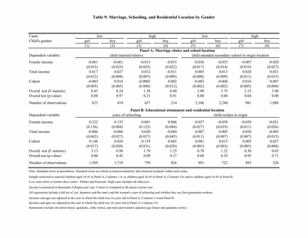
Table 9: Marriage, Schooling, and Residential Location by Gender

Caste:Child's gender: girl boy girl boy girl boy girl boy

(1) (2) (3) (4) (5) (6) (7) (8)

Dependent variable:

Female income -0.061 -0.061 -0.013 -0.015 -0.036 -0.035 -0.007 -0.020(0.032) (0.025) (0.025) (0.022) (0.017) (0.014) (0.019) (0.027)

Total income 0.017 0.027 0.012 -0.011 0.005 0.013 0.028 0.031(0.012) (0.008) (0.007) (0.009) (0.008) (0.009) (0.011) (0.015)

Cohort -0.003 0.010 -0.0002 0.002 -0.002 -0.004 0.016 0.007(0.005) (0.005) (0.008) (0.012) (0.002) (0.002) (0.005) (0.004)

Overid test (F statistic) 0.43 0.24 1.38 0.40 3.90 3.75 2.15 3.40Overid test (p-value) 0.88 0.97 0.21 0.91 0.00 0.00 0.04 0.00

Number of observations 823 419 437 214 2,106 2,240 981 1,088

Dependent variable:

Female income 0.322 0.135 0.081 0.006 -0.057 -0.030 -0.039 -0.021(0.136) (0.088) (0.125) (0.084) (0.027) (0.019) (0.011) (0.026)

Total income -0.006 -0.006 0.020 -0.060 0.007 0.005 0.020 -0.003(0.042) (0.027) (0.037) (0.045) (0.011) (0.007) (0.007) (0.015)

Cohort 0.146 0.026 0.139 0.065 0.001 0.015 0.005 0.027(0.017) (0.020) (0.031) (0.020) (0.003) (0.003) (0.005) (0.008)

Overid test (F statistic) 3.13 0.98 1.79 1.25 0.70 1.22 0.30 0.65Overid test (p-value) 0.00 0.45 0.09 0.27 0.68 0.29 0.95 0.71

Number of observations 1,589 1,719 759 826 991 722 493 326

Note: Standard errors in parentheses. Standard errors are robust to heteroscedasticity and clustered residuals within each estate.

Sample restricted to married children aged 16-45 in Panel A, Columns 1-4, to children aged 10-45 in Panel A, Columns 5-8, and to children aged 16-45 in Panel B.Low caste refers to former slave castes - Pallars and Paraiyars. High caste includes all other jatis .

Income is measured in thousands of Rupees per year. Cohort is computed as 46 minus current year.

All regressions include a full set of jati dummies and the man's and the woman's years of schooling and whether they are first-generation workers.

Incomes and ages are adjusted to the year in which the child was 16 years old in Panel A, Columns 1-4 and Panel B.Incomes and ages are adjusted to the year in which the child was 10 years old in Panel A, Columns 5-8.Instruments include elevation (linear, quadratic, cubic terms), and man and woman's adjusted age (linear and quadratic terms).

low high low high

child attended secondary school in origin location

years of schooling

Panel A: Marriage choice and school location

Panel B: Educational attainment and residential location

child married relative

child resides in origin

Table 10: Marriage, Schooling, and Residential Location by Gender (Robust Regressions)

Caste:Child's gender: girl boy girl boy girl boy girl boy

(1) (2) (3) (4) (5) (6) (7) (8)

Dependent variable:

Female income -0.044 -0.079 -0.050 -0.063 -0.113 -0.085 -0.070 -0.100(0.036) (0.043) (0.035) (0.033) (0.053) (0.033) (0.055) (0.085)

Total income 0.002 0.023 0.032 -0.014 0.051 0.062 0.064 0.082(0.017) (0.009) (0.016) (0.014) (0.025) (0.015) (0.022) (0.034)

Cohort -0.006 0.004 0.003 -0.005 -0.0003 0.002 0.025 0.018(0.007) (0.008) (0.008) (0.012) (0.003) (0.004) (0.009) (0.009)

Overid test (F statistic) 0.36 0.20 0.87 0.31 0.59 0.28 0.45 0.52Overid test (p-value) 0.87 0.96 0.50 0.91 0.70 0.92 0.81 0.76

Number of observations 823 419 437 214 2,106 2,240 981 1,088

Dependent variable:Female income 0.451 0.080 0.186 0.156 -0.078 -0.012 -0.028 -0.032

(0.243) (0.126) (0.170) (0.179) (0.049) (0.043) (0.036) (0.046)Total income -0.170 -0.033 -0.149 -0.203 0.013 -0.010 0.023 -0.004

(0.097) (0.061) (0.084) (0.066) (0.018) (0.019) (0.014) (0.025)Cohort 0.119 -0.0001 0.100 0.038 -0.002 0.013 0.005 0.028

(0.023) (0.024) (0.036) (0.038) (0.005) (0.005) (0.005) (0.008)Overid test (F statistic) 1.00 0.55 0.05 0.14 0.49 0.71 0.23 0.69Overid test (p-value) 0.42 0.74 1.00 0.98 0.78 0.62 0.95 0.64

Number of observations 1,589 1,719 759 826 991 722 493 326

Note: Standard errors in parentheses. Standard errors are robust to heteroscedasticity and clustered residuals within each estate.

Sample restricted to married children aged 16-45 in Panel A, Columns 1-4, to children aged 10-45 in Panel A, Columns 5-8, and to children aged 16-45 in Panel B.Low caste refers to former slave castes - Pallars and Paraiyars. High caste includes all other jatis .

Income is measured in thousands of Rupees per year. Cohort is computed as 46 minus current year.

All regressions include a full set of jati dummies and the man's and the woman's years of schooling and whether they are first-generation workers.

Incomes and ages are adjusted to the year in which the child was 16 years old in Panel A, Columns 1-4 and Panel B.Incomes and ages are adjusted to the year in which the child was 10 years old in Panel A, Columns 5-8.Instruments include elevation (linear, quadratic, cubic terms), and woman's adjusted age (linear and quadratic terms).The woman's adjusted age is purged of variation in marriage age across the full sample and variation in fertility across households in the same cohort.The number of children in the household and a first-boy indicator are included as controls.

low high low high

child attended secondary school in origin location

child resides in origin location

Panel A: Marriage choice and school locationchild married relative

Panel B: Educational attainment and residential location

years of schooling

Table 11: Female Autonomy

Subject:Caste: low high low high

(1) (2) (3) (4)

Could buy sari or jewellery without permission 0.30 0.34 * 0.24 0.28(0.01) (0.01) (0.01) (0.01)

Could remit money to parents without permission 0.25 0.28 * 0.22 0.24(0.01) (0.01) (0.01) (0.01)

Collects her own salary (all workers) 0.14 0.19 * -- --(0.01) (0.01)

Collects her own salary (husband works on estate) 0.07 0.09 * -- --(0.01) (0.01)

No. of observations 2,509 1,178 2,403 1,116

Note: standard errors in parentheses. Low castes include Pallars and Paraiyars. High castes include all other jatis .Each autonomy question is coded as a binary variable, which takes the value one if the response is "yes" and zero if "no."The question whether the worker collects her own salary is coded separately for all workers and for those whose husbands work on the estates.

female workers mothers of female workers