B ezier Curves - Brigham Young Universitycagd.cs.byu.edu/~557/text/ch2.pdf · 3 = 0. This explains...

Chapter 2

Bezier Curves

Bezier curves are named after their inventor, Dr. Pierre Bezier, an engineer with the Renault carcompany who set out in the early 1960’s to develop a curve formulation for use in shape designthat would be intuitive enough for designers and artists to use, without requiring a background inmathematics.

Figure 2.1: Examples of cubic Bezier curves.

Figure 2.1 shows three different Bezier curves, with their corresponding control polygons. Eachcontrol polygon is comprised of four control points that are connect with line segments. (Thesecontrol polygons are not closed, and might more properly be called polylines.) The beauty of theBezier representation is that a Bezier curve mimics the shape of its control polygon. A Beziercurve passes through its first and last control points, and is tangent to the control polygon at thoseendpoints. An artist can quickly master the process of designing shapes using Bezier curves bymoving the control points, and most 2D drawing systems like Adobe Illustrator use Bezier curves.

Complicated shapes can be created by using a sequence of Bezier curves. Since Bezier curves aretangent to their control polygons, it is easy to join together two Bezier curves such that they aretangent continuous. Figure 2.2 shows the outline of a letter “g” created using several Bezier curves.All PostScript font outlines are defined using Bezier curves. Hence, as you read these notes, you aregazing upon Bezier curves!

Although Bezier curves can be used productively by artists who have little mathematical training,

17

18 The Equation of a Bezier Curve

Figure 2.2: Font definition using Bezier curves.

one of the main objectives in this course is to study the underlying mathematics. These notes attemptto show that the power and elegance of Bezier curves are matched by the beauty of the underlyingmathematics.

2.1 The Equation of a Bezier Curve

The equation of a Bezier curve is similar to the equation for the center of mass of a set of pointmasses. Consider the four masses m0, m1, m2, and m3 in Figure 2.3.a located at points P0, P1, P2,P3.

P0

P1 P2

P3

P

(a) Center of mass of four points.

P0

P1 P2

P3(b) Cubic Bezier Curve.

Figure 2.3: Bezier Curves in Terms of Center of Mass.

The equation for the center of mass is

P =m0P0 + m1P1 + m2P2 + m3P3

m0 + m1 + m2 + m3.

Next, imagine that instead of being fixed, constant values, each mass varies as a function of aparameter t. Specifically, let

m0(t) = (1− t)3, m1(t) = 3t(1− t)2, m2(t) = 3t2(1− t), m3(t) = t3. (2.1)

Now, for each value of t, the masses assume different weights and their center of mass changescontinuously. As t varies between 0 and 1, a curve is swept out by the moving center of mass.

T. W. Sederberg, BYU, Computer Aided Geometric Design Course Notes September 21, 2016

The Equation of a Bezier Curve 19

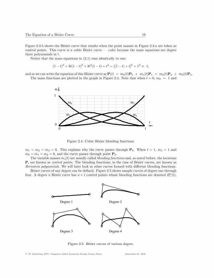
Figure 2.3.b shows the Bezier curve that results when the point masses in Figure 2.3.a are taken ascontrol points. This curve is a cubic Bezier curve — cubic because the mass equations are degreethree polynomials in t.

Notice that the mass equations in (2.1) sum identically to one:

(1− t)3 + 3t(1− t)2 + 3t2(1− t) + t3 = [(1− t) + t]3 = 13 ≡ 1,

and so we can write the equation of this Bezier curve as P(t) = m0(t)P0 + m1(t)P1 + m2(t)P2 + m3(t)P3.The mass functions are plotted in the graph in Figure 2.4. Note that when t = 0, m0 = 1 and

m

1

00 1

t

m0

m1 m2

m3

Figure 2.4: Cubic Bezier blending functions.

m1 = m2 = m3 = 0. This explains why the curve passes through P0. When t = 1, m3 = 1 andm0 = m1 = m2 = 0, and the curve passes through point P3.

The variable masses mi(t) are usually called blending functions and, as noted before, the locationsPi are known as control points. The blending functions, in the case of Bezier curves, are known asBernstein polynomials. We will later look at other curves formed with different blending functions.

Bezier curves of any degree can be defined. Figure 2.5 shows sample curves of degree one throughfour. A degree n Bezier curve has n+ 1 control points whose blending functions are denoted Bni (t),

Degree 1 Degree 2

Degree 3 Degree 4

Figure 2.5: Bezier curves of various degree.


20 Bezier Curves over Arbitrary Parameter Intervals

where

Bni (t) =

(n

i

)(1− t)n−iti, i = 0, 1, ..., n.

Recall that (n

i

)=

n!

i!(n− i)!.(

ni

)is spoken “n – choose – i” and is called a binomial coefficient because it arises in the binomial

expansion

(a+ b)n =

n∑i=0

(n

i

)aibn−i.

In the degree three case, n = 3 and B30 = (1− t)3, B3

1 = 3t(1− t)2, B32 = 3t2(1− t) and B3

3 = t3.Bni (t) is also referred to as the ith Bernstein polynomial of degree n. The equation of a Bezier curveis thus:

P(t) =

n∑i=0

(n

i

)(1− t)n−itiPi. (2.2)

2.2 Bezier Curves over Arbitrary Parameter Intervals

Equation 2.2 gives the equation of a Bezier curve which starts at t = 0 and ends at t = 1. It isuseful, especially when fitting together a string of Bezier curves, to allow an arbitrary parameterinterval:

t ∈ [t0, t1]

such that P(t0) = P0 and P(t1) = Pn. We will denote the Bezier curve defined over an arbitraryparameter interval by P[t0,t1](t). It’s equation is a modification of (2.2):

P[t0,t1](t) =

∑ni=0

(ni

)(t1 − t)n−i(t− t0)iPi

(t1 − t0)n=

n∑i=0

(n

i

)(t1 − tt1 − t0

)n−i(t− t0t1 − t0

)iPi. (2.3)

If no parameter interval is specified, it is assumed to be [0, 1]. That is,

P(t) = P[0,1](t).

2.3 The de Casteljau Algorithm

The de Casteljau algorithm describes how to subdivide a Bezier curve P[t0,t2] into two segmentsP[t0,t1] and P[t1,t2] whose union is equivalent to P[t0,t2]. This algorithm was devised in 1959 by Paulde Casteljau, a French mathematician at the Citroen automobile company. It is an example of ageometric construction algorithm.

To facilitate our description of the algorithm, we label the control points of a cubic Bezier curveP[t0,t2] with P0

0, P01, P0

2, and P03 as illustrated in Figure 2.6. The algorithm involves computing the

sequence of points

Pji = (1− τ)Pj−1

i + τPj−1i+1 ; j = 1, . . . , n; i = 0, . . . , n− j. (2.4)


The de Casteljau Algorithm 21

P00

P10

P20

P30

P01

P11

P21

P02

P12

P03

! = .4

P00

P10

P20

P30

P01

P11

P21

P02

P12

P03

! = .6

Figure 2.6: Subdividing a cubic Bezier curve.

where τ = t1−t0t2−t0 . Then, the control points for P[t0,t1](t) are P0

0,P10,P

20, . . . ,P

n0 and the control

points for P[t1,t2](t) are Pn0 ,P

n−11 ,Pn−2

2 , . . . ,P0n. Although our example is for a cubic Bezier curve

(n = 3), the algorithm works for any degree.A practical application of the de Casteljau algorithm is that it provides a numerically stable means

of computing the coordinates and tangent vector of any point along the curve, since P(t1) = Pn0

and the tangent vector is Pn−11 −Pn−1

0 .Figure 2.7 shows that when a Bezier curve is repeatedly subdivided, the collection of control

polygons converge to the curve. Thus, one way of plotting a Bezier curve is to simply subdivide it

1 curve 2 curves

4 curves 8 curves

Figure 2.7: Recursively subdividing a quadratic Bezier curve.

an appropriate number of times and plot the control polygons (although a more efficient way is touse Horner’s algorithm (see Chapter 3) or forward differencing (see Chapter 4)).

The de Casteljau algorithm works even if τ 6∈ [0, 1], which is equivalent to t1 6∈ [t0, t2]. Fig. 2.8shows a quadratic Bezier curve “subdivided” at τ = 2. The de Castelau algorithm is numericallystable as long as the parameter subdivision parameter is within the parameter domain of the curve.


22 Degree Elevation

P00

P10

P20

P01

P11

P02

! = 2

Figure 2.8: Subdividing a quadratic Bezier curve.

2.4 Degree Elevation

Any degree n Bezier curve can be exactly represented as a Bezier curve of degree n+ 1 (and hence,as a curve of any degree m > n). Given a degree n Bezier curve, the procedure for computing thecontrol points for the equivalent degree n+ 1 Bezier curve is called degree elevation.

We now derive the degree elevation formula, using the identities:

(1− t)Bni (t) = (1− t)(n

i

)(1− t)n−iti

=

(n

i

)(1− t)n−i+1ti

=

(ni

)(n+1i

)(n+ 1

i

)(1− t)n−i+1ti

=

(ni

)(n+1i

)Bn+1i =

n!i!(n−i)!(n+1)!

i!(n+1−i)!

Bn+1i

=n!i!(n+ 1− i)!i!(n− i)!(n+ 1)!

Bn+1i =

n!i!(n+ 1− i)(n− i)!i!(n− i)!(n+ 1)n!

Bn+1i

=n+ 1− in+ 1

Bn+1i (2.5)

and

tBni (t) =i+ 1

n+ 1Bn+1i+1 (t). (2.6)

Degree elevation is accomplished by simply multiplying the equation of the degree n Bezier curve


Degree Elevation 23

by [(1− t) + t] = 1:

P(t) = [(1− t) + t]P(t)

= [(1− t) + t]

n∑i=0

PiBni (t)

=

n∑i=0

Pi[(1 + t)Bni (t) + tBni (t)]

=

n∑i=0

Pi[n+ 1− in+ 1

Bn+1i +

i+ 1

n+ 1Bn+1i+1 (t)]

=

n∑i=0

n+ 1− in+ 1

PiBn+1i +

n∑i=0

i+ 1

n+ 1PiB

n+1i+1 (t)

=

n∑i=0

n+ 1− in+ 1

PiBn+1i +

n+1∑i=1

i

n+ 1Pi−1B

n+1i (t)

=

n+1∑i=0

n+ 1− in+ 1

PiBn+1i +

n+1∑i=0

i

n+ 1Pi−1B

n+1i (t)

=

n+1∑i=0

[(n+ 1− i)Pi + iPi−1

n+ 1]Bn+1i (t)

=

n+1∑i=0

P∗iBn+1i (t) (2.7)

where

P∗i = αiPi−1 + (1− αi)Pi, αi =i

n+ 1. (2.8)

P0* P0

1/4

1/2

P1*

P1 old P2* P2

P3*

P4*P3

new

(a) Degree Elevation of a Cubic Bezier Curve.

Degree 2 Degree 3 Degree 4

Degree 5 Degree 6 Degree 7

(b) Repeated degree elevation.

Figure 2.9: Degree Elevation of a Bezier Curve.


24 The Convex Hull Property of Bezier Curves

For the case n = 3, the new control points P∗i are:

P∗0 = P0

P∗1 =1

4P0 +

3

4P1

P∗2 =2

4P1 +

2

4P2

P∗3 =3

4P2 +

1

4P3

P∗4 = P3

Figure 2.9.a illustrates.If degree elevation is applied repeatedly, as shown in Figure 2.9.b, the control polygon converges

to the curve itself.

2.5 The Convex Hull Property of Bezier Curves

An important property of Bezier curves is that they always lie within the convex hull of their controlpoints. The convex hull can be envisioned by pounding an imaginary nail into each control point,stretching an imaginary rubber band so that it surrounds the group of nails, and then collapsing thatrubber band around the nails. The polygon created by that imaginary rubber band is the convexhull. Figure 2.10 illustrates.

The fact that Bezier curves obey the convex hull property is assured by the center-of-massdefinition of Bezier curves in Section 2.1. Since all of the control points lie on one side of an edgeof the convex hull, it is impossible for the center of mass of those control points to lie on the otherside of the line,

P0

P1 P2

P3

P0

P1

P2

P3

P0

P1P2

P3

P0 P1 P2

P3

Figure 2.10: Convex Hull Property


Distance between Two Bezier Curves 25

2.6 Distance between Two Bezier Curves

The problem often arises of determining how closely a given Bezier curve is approximated by asecond Bezier curve. For example, if a given cubic curve can be adequately represented by a degreeelevated quadratic curve, it might be advantageous to replace the cubic curve with the quadratic.

Given two Bezier curves

P(t) =

n∑i=0

PiBni (t); Q(t) =

n∑i=0

QiBni (t)

the vector P(t) − Q(t) between points of equal parameter value on the two curves can itself beexpressed as a Bezier curve

D(t) = P(t)−Q(t) =

n∑i=0

(Pi −Qi)Bni (t)

whose control points are Di = Pi−Qi. The vector from the origin to the point D(t) is P(t)−Q(t).The convex hull property guarantees that the distance between the two curves is bounded by thelargest distance from the origin to any of the control points Di.

P0

P1 P2

P3Q0

Q1 Q2

Q3

t=1/2

P3-Q3

P2-Q2

P1-Q1

P0-Q0

Figure 2.11: Difference curve.

This error bound is attractive because it is very easy to compute. However, it is not always avery tight bound because it is dependent on parametrization.

A more precise statement of the distance between two curves is the Hausdorff distance. Giventwo curves P[s0,s1](s) and Q[t0,t1](t). The Hausdorff distance d(P,Q) is defined

d(P,Q) = maxs∈[s0,s1]

{min

t∈[t0,t1]|P(s)−Q(t)|

}(2.9)

where |P(s)−Q(t)| is the Euclidean distance between a point P(s) and the point Q(t). In practice,it is much more expensive to compute the Hausdorff distance than to compute a bound using thedifference curve in Figure 2.11.


26 Derivatives

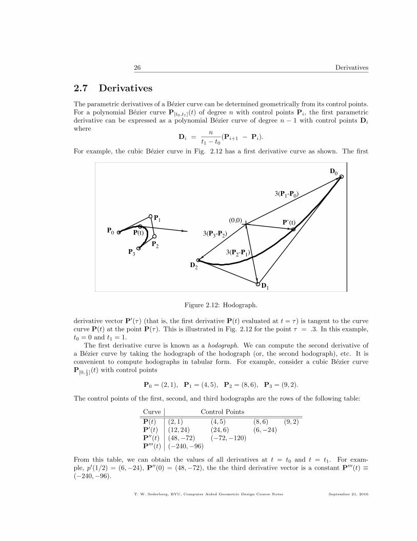
2.7 Derivatives

The parametric derivatives of a Bezier curve can be determined geometrically from its control points.For a polynomial Bezier curve P[t0,t1](t) of degree n with control points Pi, the first parametricderivative can be expressed as a polynomial Bezier curve of degree n − 1 with control points Di

whereDi =

n

t1 − t0(Pi+1 − Pi).

For example, the cubic Bezier curve in Fig. 2.12 has a first derivative curve as shown. The first

P0

P1

P2P3

P(t)

D0

D1

D2

3(P1-P0)

3(P2-P1)

3(P3-P2)P’(t)(0,0)

Figure 2.12: Hodograph.

derivative vector P′(τ) (that is, the first derivative P(t) evaluated at t = τ) is tangent to the curvecurve P(t) at the point P(τ). This is illustrated in Fig. 2.12 for the point τ = .3. In this example,t0 = 0 and t1 = 1.

The first derivative curve is known as a hodograph. We can compute the second derivative ofa Bezier curve by taking the hodograph of the hodograph (or, the second hodograph), etc. It isconvenient to compute hodographs in tabular form. For example, consider a cubic Bezier curveP[0, 12 ]

(t) with control points

P0 = (2, 1), P1 = (4, 5), P2 = (8, 6), P3 = (9, 2).

The control points of the first, second, and third hodographs are the rows of the following table:

Curve Control Points

P(t) (2, 1) (4, 5) (8, 6) (9, 2)P′(t) (12, 24) (24, 6) (6,−24)P′′(t) (48,−72) (−72,−120)P′′′(t) (−240,−96)

From this table, we can obtain the values of all derivatives at t = t0 and t = t1. For exam-ple, p′(1/2) = (6,−24), P′′(0) = (48,−72), the the third derivative vector is a constant P′′′(t) ≡(−240,−96).


Three Dimensional Bezier Curves 27

It is noteworthy that if the hodograph passes through the origin, there is a cusp correspondingto that point on the original curve!

Note that the hodograph we have just described relates only to polynomial Bezier curves, notto rational Bezier curves or any other curve that we will study. The derivative of any other curvemust be computed by differentiation. For a rational Bezier curve, that differentiation will involvethe quotient rule. Consequently, the derivative of a degree n rational Bezier curve can be expressedas a rational Bezier curve of degree 2n. As it turns out, the equations for those control points arerather messy.

2.8 Three Dimensional Bezier Curves

If Bezier control points are defined in three dimensional space, the resulting Bezier curve is threedimensional. Such a curve is sometimes called a space curve, and a two dimensional curve is calleda planar curve. Our discussion of the de Casteljau algorithm, degree elevation, and hodographsextend to 3D without modification.

Since a degree two Bezier curve is defined using three control points, every degree two curve isplanar, even if the control points are in a three dimensional coordinate system.

2.9 Rational Bezier Curves

A rational Bezier curve is one for which each control point Pi is assigned a scalar weight. Theequation of a rational Bezier curve is ∑n

i=0 wiBni (t)Pi∑n

i=0 wiBni (t)

.

The effect of changing a control point weight is illustrated in Fig. 2.13. This type of curve is knownas a rational Bezier curve, because the blending functions are rational polynomials, or the ratio oftwo polynomials. Note that if all weights are 1 (or if all weights are simply the same), a rationalBezier curve reduces to a polynomial Bezier curve.

Rational Bezier curves have several advantages over polynomial Bezier curves. Clearly, rationalBezier curves provide more control over the shape of a curve than does a polynomial Bezier curve.In addition, a perspective drawing of a 3D Bezier curve (polynomial or rational) is a rational Beziercurve, not a polynomial Bezier curve. Also, rational Bezier curves are needed to exactly expressall conic sections. A degree two polynomial Bezier curve can only represent a parabola. Exactrepresentation of circles requires rational degree two Bezier curves.

A rational Bezier curve can be interpreted as the perspective projection of a 3-D polynomialcurve. Fig. 2.14 shows two curves: a 3-D curve and a 2-D curve. The 2-D curve lies on the planez = 1 and it is defined as the projection of the 3-D curve onto the plane z = 1. One way to considerthis is to imagine a funny looking cone whose vertex is at the origin and which contains the 3-Dcurve. In other words, this cone is the collection of all lines which contain the origin and a point onthe curve. Then, the 2-D rational Bezier curve is the intersection of the cone with the plane z = 1.

What we see here can be viewed as the geometric interpretation of homogeneous coordinates dis-cussed in Section 7.1.1. The 3D Bezier control points wi(xi, yi, 1) = (xiwi, yiwi, wi) can be thoughtof as homogeneous coordinates (X,Y, Z) that correspond to 2D Cartesian coordinates (XZ ,

YZ ). If the

2-D rational Bezier curve has control points (xi, yi) with corresponding weights wi, then the homo-geneous (X,Y, Z) coordinates of the 3-D control points are wi(xi, yi, 1) = (xiwi, yiwi, wi). Denote


28 Rational Bezier Curves

P0

P1

P2

P3

w2=0

w2=.5

w2=1

w2=2

w2=5 w2=10

Figure 2.13: Rational Bezier curve.

points on the 3-D curve using upper case variables (X(t), Y (t), Z(t)) and on the 2-D curve usinglower case variables (x(t), y(t)). Then, any point on the 2-D rational Bezier curve can be computedby computing the corresponding point on the 3-D curve, (X(t), Y (t), Z(t)), and projecting it to theplane z = 1 by setting

x(t) =X(t)

Z(t), y(t) =

Y (t)

Z(t).

2.9.1 De Casteljau Algorithm and Degree Elevation on Rational BezierCurves

The de Casteljau algorithm and degree elevation algorithms for polynomial Bezier curves extend eas-ily to rational Bezier curves as follows. First, convert the rational Bezier curve into its correspondingpolynomial 3D Bezier curve as discussed in Section 2.9. Next, perform the de Casteljau algorithmor degree elevation on the 3D polynomial Bezier curve. Finally, map the resulting 3D Bezier curveback to 2D. The Z coordinates of the control points end up as the weights of the control points forthe 2D rational Bezier curve.

This procedure does not work for hodographs, since the derivative of a rational Bezier curverequires the use of the quotient rule for differentiation. However, Section 2.9.2 describes how tocompute the first derivative at the endpoint of a rational Bezier curve and Section 2.9.3 describeshow to compute the curvature at the endpoint of a rational Bezier curve. Used in conjunction withthe de Casteljau algorithm, this enable us to compute the first derivative or curvature at any pointon a rational Bezier curve.


Rational Bezier Curves 29

x

y

z

z=1

(x0,y0,1)w0

(x1,y1,1)w1

(x2,y2,1)w2

(x3,y3,1)w3

(x0,y0,1)

(x1,y1,1)(x2,y2,1)

(x3,y3,1)

z

x

z=1

xiwi

xi

wi

1

Figure 2.14: Rational curve as the projection of a 3-D curve.


30 Rational Bezier Curves

2.9.2 First Derivative at the Endpoint of a Rational Bezier Curve

The derivative equation for a rational Bezier involves the quotient rule for derivatives — it does notwork to simply compute the tangent vector and curvature for the three dimensional non-rationalBezier curve and then project that value to the (x, y) plane. For a degree n rational Bezier curveP[0,1](t),

x(t) =xn(t)

d(t)=

w0x0(n0

)(1− t)n + w1x1

(n1

)(1− t)n−1t+ w2x2

(n2

)(1− t)n−2t2 + . . .

w0

(n0

)(1− t)n + w1

(n1

)(1− t)n−1t+ w2

(n2

)(1− t)n−2t2 + . . .

;

y(t) =yn(t)

d(t)=

w0y0(n0

)(1− t)n + w1y1

(n1

)(1− t)n−1t+ w2y2

(n2

)(1− t)n−2t2 + . . .

w0

(n0

)(1− t)n + w1

(n1

)(1− t)n−1t+ w2

(n2

)(1− t)n−2t2 + . . .

the equation for the first derivative vector at t = 0 must be found by evaluating the followingequations:

x(0) =d(0)xn(0)− d(0)xn(0)

d2(0); y(0) =

d(0)yn(0)− d(0)yn(0)

d2(0)

from which

P′(0) =w1

w0n(P1 −P0). (2.10)

For a rational curve P[t0,t1](t), the first derivative at t = t0 is:

P′(t0) =w1

w0

n

t1 − t0(P1 −P0). (2.11)

The second derivative of a rational Bezier curve at its endpoint is

P′′(t0) =n(n− 1)

(t1 − t0)2w2

w0(P2 −P0)− 2n

(t1 − t0)2w1

w0

nw1 − w0

w0(P1 −P0) (2.12)

2.9.3 Curvature at an Endpoint of a Rational Bezier Curve

The curvature (denoted by κ) of a curve is a measure of how sharply it curves. The curvature of acircle of radius ρ is defined to be κ = 1/ρ. A straight line does not curve at all, and its curvature iszero. For other curves, the curvature is generally different at each point on the curve. The meaningof curvature in this general case is illustrated by Figure 2.15 which shows a Bezier curve and theosculating circle with respect to a point on the curve. The word “osculate” means to kiss, and theosculating circle is the circle that “best fits” the curve at a particular point in the following sense.An arbitrary line that passes through a point on a curve intersects the curve with multiplicity one;the tangent line at that point intersects the curve with multiplicity two. An osculating circle is acircle of radius ρ that intersects the curve with multiplicity at least three, and the curvature κ isdefined to be κ = 1/ρ. (See Section 7.3.1 for a description of intersection multiplicity.) ρ is calledthe radius of curvature for the curve at that point.

In Figure 2.15, the center of the circle, C, is located along the normal line a distance ρ from thepoint of contact.


Rational Bezier Curves 31

Cρ

Tangent line

(a) At t = .7 (b) At t = .1 (c) At t = .8

Figure 2.15: Osculating Circles.

The equation for the curvature of a parametric curve is

κ =|xy − yx|

(x2 + y2)32

where the dots denote differentiation with respect to the curve parameter. If this equation is appliedto an endpoint of a rational Bezier curve, a beautifully simple and geometrically meaningful equationresults:

κ(t0) =w0w2

w21

n− 1

n

h

a2(2.13)

where n is the degree of the curve and a and h are as shown in Fig. 2.16 (a is the length of the firstleg of the control polygon, and h is the perpendicular distance from P2 to the first leg of the controlpolygon). Curvature is independent of [t0, t1].

a

h P0

P1

P2

Figure 2.16: Endpoint curvature.

While is is mathematically possible to write down an equation for the first derivative vector andfor the curvature of a rational Bezier curve as a function of t, such equations would be extremelycomplicated. The best way to find the curvature or first derivative vector at an arbitrary point


32 Continuity

along a rational Bezier curve is to first perform the de Casteljau algorithm (Section 2.3) to makethe desired point an endpoint of the curve, and then apply (2.11) or (2.13).

Example A rational quadratic Bezier curve has control points and weights:

P0 = (0, 0), w0 = 1; P1 = (4, 3), w1 = 2; P2 = (0, 5), w2 = 4.

What is the curvature at t = 0?

SolutionThe distance equation for the line P0P1 is 3

5x −45y, so plugging the Cartesian coordinates of P2

into this distance equation give h = 4. The value of a is found as the distance from P0 to P1, whichis√

42 + 32 = 5. So, the curvature is

κ(0) =w0w2

w21

n− 1

n

h

a2=

1 · 422

1

2

4

52=

2

25

2.10 Continuity

Two curve segments P[t0,t1] and Q[t1,t2] are said to be Ck continuous (or, to have kth order parametriccontinuity) if

P(t1) = Q(t1), P′(t1) = Q′(t1), . . . , P(k)(t1) = Q(k)(t1). (2.14)

Thus, C0 means simply that the two adjacent curves share a common endpoint. C1 means that thetwo curves not only share the same endpoint, but also that they have the same tangent vector attheir shared endpoint, in magnitude as well as in direction. C2 means that two curves are C1 andin addition that they have the same second order parametric derivatives at their shared endpoint,both in magnitude and in direction.

In Fig. 2.17, the two curves P[t0,t1](t) and Q[t1,t2](t) are at least C0 because p3 ≡ q0. Further-

p0

p1

p2 p3 q0 q1

q2

q3

Figure 2.17: C2 Bezier curves.

more, they are C1 if3

t1 − t0(p3 − p2) =

3

t2 − t1(q1 − q0).


Curvature Combs 33

They are C2 if they are C1 and

6

(t1 − t0)2(p3 − 2p2 + p1) =

6

(t2 − t1)2(q2 − 2q1 + q0).

A second method for describing the continuity of two curves, that is independent of theirparametrization, is called geometric continuity and is denoted Gk. The conditions for geometriccontinuity (also known as visual continuity) are less strict than for parametric continuity. For G0

continuity, we simply require that the two curves have a common endpoint, but we do not requirethat they have the same parameter value at that common point. For G1, we require that line seg-ments p2 − p3 and q0 − q1 are collinear, but they need not be of equal length. This means thatthey have a common tangent line, though the magnitude of the tangent vector may be different. G2

(second order geometric continuity) means that the two neighboring curves have the same tangentline and also the same center of curvature at their common boundary. A general definition of Gn isthat two curves that are Gn can be reparametrized (see Section 2.13) to make them be Cn. Twocurves which are Cn are also Gn, as long as (2.15) holds.

P(t1) = Q(t1), P′(t1) = Q′(t1) 6= 0, . . . , P(k)(t1) = Q(k)(t1) 6= 0. (2.15)

Second order continuity (C2 or G2) is often desirable for both physical and aesthetic reasons.One reason that cubic NURBS curves and surfaces are an industry standard in CAD is that theyare C2. Two surfaces that are G1 but not G2 do not have smooth reflection lines. Thus, a car bodymade up of G1 surfaces will not look smooth in a show room. Railroad cars will jerk where G1

curves meet.

2.11 Curvature Combs

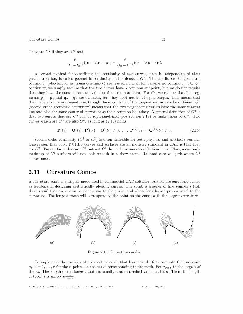
A curvature comb is a display mode used in commercial CAD software. Artists use curvature combsas feedback in designing aesthetically pleasing curves. The comb is a series of line segments (callthem teeth) that are drawn perpendicular to the curve, and whose lengths are proportional to thecurvature. The longest tooth will correspond to the point on the curve with the largest curvature.

(a) (b) (c) (d)

Figure 2.18: Curvature combs.

To implement the drawing of a curvature comb that has n teeth, first compute the curvatureκi, i = 1, . . . , n for the n points on the curve corresponding to the teeth. Set κmax to the largest ofthe κi. The length of the longest tooth is usually a user-specified value, call it d. Then, the lengthof tooth i is simply d κi

κmax.


34 Circular Arcs

As a general rule, artists consider that the most aesthetically pleasing curves have curvaturecombs whose length changes monotonically and smoothly. The line segments are drawn in thedirection away from the center of curvature, as illustrated in Figure 2.18.

The continuity of two curves P and Q can be visualized in terms of their respective curvaturecombs. Define a comb curve to be the set of endpoints of a comb. Denote by Pc the curve combof P and by Qc the curve comb of Q. Then, if P and Q are G1, Pc and Qc are discontinuous, asshown in Figure 2.19.a. If P and Q are G2, Pc and Qc are G0, as shown in Figure 2.19.b.

(a) Original curves are G1. Comb curves are discon-tinuous.

(b) Original curves are G2. Comb curves are G0.

Figure 2.19: Curvature combs for two piecewise curves.

To get comb curves that are mathematically G1, P and Q must be G3. In practice, somecommercial software advertises that their curves and surfaces are G3 or C3. This is often marketingjargon; what they really mean is that the curvature combs look like they are G1 when in reality, Pand Q may not even be exactly G1 or even G0.

2.12 Circular Arcs

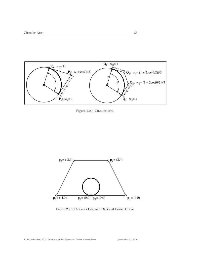
Circular arcs can be exactly represented using rational Bezier curves. Figure 2.20 shows a circulararc as both a degree two and a degree three rational Bezier curve. Of course, the control polygonsare tangent to the circle. The degree three case is a simple degree elevation of the degree two case.The length e is given by

e =2 sin θ

2

1 + 2 cos θ2r.

The degree two case has trouble when θ approaches 180◦ since P1 moves to infinity, although thiscan be remedied by just using homogeneous coordinates. The degree three case has the advantagethat it can represent a larger arc, but even here the length e goes to infinity as θ approaches 240◦.For large arcs, a simple solution is to just cut the arc in half and use two cubic Bezier curves. Acomplete circle can be represented as a degree five Bezier curve as shown in Figure 2.21. Here, theweights are w0 = w5 = 1 and w1 = w2 = w3 = w4 = 1

5 .


Circular Arcs 35

θ

P1; w1= cos(θ/2)

P0; w0= 1

P2; w2= 1

d

r

θ

Q1; w1= (1 + 2cos(θ/2))/3

Q0; w0= 1

Q2; w2= (1 + 2cos(θ/2))/3

Q3; w3= 1

e

e

r

Figure 2.20: Circular arcs.

p0 = (0,0) p1 = (4,0)

p2 = (2,4)p3 = (-2,4)

p4 = (-4,0) p5 = (0,0)

Figure 2.21: Circle as Degree 5 Rational Bezier Curve.


36 Reparametrization of Bezier Curves

2.13 Reparametrization of Bezier Curves

Reparametrization of a curve means to change how a curve is parametrized, i.e., to change whichparameter value is assigned to each point on the curve. Reparametrization can be performed by aparameter substitution. Given a parametric curve P(t), if we make the substitution t = f(s), weend up with a curve Q(s) which is geometrically identical to P(t). For example, let

P(t) = (t2 + t− 1, 2t2 − t+ 3), t = 2s+ 1

yields

Q(s) = ((2s+ 1)2 + (2s+ 1)− 1, 2(2s+ 1)2 − (2s+ 1) + 3) = (4s2 + 6s+ 1, 8s2 + 6s+ 4).

The curves P(t) and Q(s) consist of the same points (if the domains are infinite) but the correspon-dence between parameter values and points on the curve are different.

A simple (and obvious) way to reparametrize a Bezier curve P[t0,t1](t) is to simply change thevalues of t0 and t1 without changing the control points. Thus, two curves P[t0,t1](t) and Q[s0,s1](s)that have the same degree, control point positions, and weights, but for which t0 6= s0 and/or t1 6= s1are reparametrizations of each other. The reparametrization function is

t =t0s1 − s0t1s1 − s0

+t1 − t0s1 − s0

s, or s =s0t1 − t0s1t1 − t0

+s1 − s0t1 − t0

t.

ExampleBezier curves P[0,1](t) and Q[5,9](s) have the same degree, control point positions, and weights. Thecurves look the same, but have different parametrizations. For example,

P(0) = Q(5), P(1) = Q(9), P(.5) = Q(7).

In general,

P(t) ≡ Q(5 + 4t) and Q(s) ≡ P(−5

4+

1

4s).

A rational parametric curve can be reparametrized with the substitution t = f(u)/g(u). Inthis case, it is possible to perform a rational-linear reparametrization which does not change theendpoints of the curve segment. If we let

t =a(1− u) + bu

c(1− u) + du

and want u = 0 when t = 0 and u = 1 when t = 1, then a = 0 and b = d. Since we can scale thennumerator and denominator without affecting the reparametrization, set c = 1 and we are left with

t =bu

(1− u) + bu

A rational Bezier curve

X(t) =

(n0

)w0P0(1− t)n +

(n1

)w1P1(1− t)n−1t + ... +

(nn

)wnPnt

n(n0

)w0(1− t)n +

(n1

)w1(1− t)n−1t + ... +

(nn

)wntn

can be raparametrized without changing its endpoints by making the substitutions

t =bu

(1− u) + bu, (1− t) =

(1− u)

(1− u) + bu.


Advantages of Rational Bezier Curves 37

After multiplying numerator and denominator by ((1− u) + bu)n, we obtain

X(u) =

(n0

)(b0w0)P0(1− u)n +

(n1

)(b1w1)P1(1− u)n−1u + ... +

(nn

)(bnwn)Pnu

n(n0

)b0w0(1− u)n +

(n1

)b1w1(1− u)n−1u + ... +

(nn

)bnwnun

In other words, if we scale the weights wi by bi, the curve will not be changed!

Negative Weights

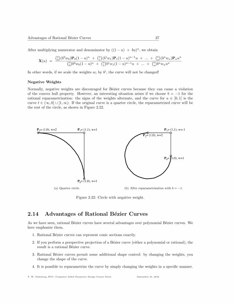
Normally, negative weights are discouraged for Bezier curves because they can cause a violationof the convex hull property. However, an interesting situation arises if we choose b = −1 for therational reparametrization: the signs of the weights alternate, and the curve for u ∈ [0, 1] is thecurve t ∈ (∞, 0] ∪ [1,∞). If the original curve is a quarter circle, the reparametrized curve will bethe rest of the circle, as shown in Figure 2.22.

P0= (1,0), w=1

P1= (1,1), w=1P2= (1,0), w=2

(a) Quarter circle.

P0= (1,0), w=1

P1= (1,1), w=-1

P2= (1,0), w=2

(b) After reparametrization with b = −1.

Figure 2.22: Circle with negative weight.

2.14 Advantages of Rational Bezier Curves

As we have seen, rational Bezier curves have several advantages over polynomial Bezier curves. Wehere emphasize them.

1. Rational Bezier curves can represent conic sections exactly.

2. If you perform a perspective projection of a Bezier curve (either a polynomial or rational), theresult is a rational Bezier curve.

3. Rational Bezier curves permit some additional shape control: by changing the weights, youchange the shape of the curve.

4. It is possible to reparametrize the curve by simply changing the weights in a specific manner.


38 Explicit Bezier Curves

2.15 Explicit Bezier Curves

An explicit Bezier curve P[t0,t1](t) is one for which x ≡ t. For a polynomial Bezier curve, thishappens when the x-coordinates of the control points are evenly spaced between t0 and t1. That is,

Pi = ( t0(n−i)+t1in , yi), i = 0, . . . , n. Such a Bezier curve takes on the form of a function

x = t

y = f(t)

or simplyy = f(x).

An explicit Bezier curve is sometimes called a non-parametric Bezier curve. It is just a polynomialfunction expressed in the Bernstein polynomial basis. Figure 2.23 shows a degree five explicit Beziercurve over the domain [t0, t1] = [0, 1].

P0

P1

P2

P3

P4P5

0.2

.4 .6 .8 1

Figure 2.23: Explicit Bezier curve.

It is also possible to create an explicit rational Bezier curve. However, the representation of adegree-n rational function

x = t; y =

∑ni=0 wiyiB

ni (t)∑n

i=0 wiBni (t)

as an explicit Bezier curve is degree n+ 1 because we must have

x = t = t

∑ni=0 wiB

ni (t)∑n

i=0 wiBni (t)

which is degree n+ 1. Since x(t) is degree n+ 1, we must likewise degree elevate y(t).

2.16 Integrating Bernstein polynomials

Recall that the hodograph (first derivative) of a Bezier curve is easily found by simply differencingadjacent control points (Section 2.7). It is equally simple to compute the integral of a Bernstein


Integrating Bernstein polynomials 39

polynomial. Since the integral of a polynomial in Bernstein form

p(t) =

n∑i=0

piBni (t) (2.16)

is that polynomial whose derivative is p(t). If the desired integral is a degree n + 1 polynomial inBernstein form

q(t) =

n+1∑i=0

qiBn+1i (t), (2.17)

we havepi = (n+ 1)(qi+1 − qi). (2.18)

Hence, q0 = 0 and

qi =

∑i−1j=0 pj

n+ 1, i = 1, n+ 1. (2.19)

Note that if p(t) is expressed as an explicit Bezier curve, q(t) can be interpreted as the area underp(t) between the lines x = 0 and x = t. Thus, the entire area under an explicit Bezier curve can becomputed as simply the average of the control points! This is so because

q(1) = qn+1 =

∑nj=0 pj

n+ 1. (2.20)


B ezier Curves - Brigham Young Universitycagd.cs.byu.edu/~557/text/ch2.pdf · 3 = 0. This explains...

Documents

Transcript of B ezier Curves - Brigham Young Universitycagd.cs.byu.edu/~557/text/ch2.pdf · 3 = 0. This explains...