ORIGINAL ARTICLE

Axonal morphometry of hippocampal pyramidal neuronssemi-automatically reconstructed after in vivo labelingin different CA3 locations

Deepak Ropireddy • Ruggero Scorcioni •

Bonnie Lasher • Gyorgy Buzsaki • Giorgio A. Ascoli

Received: 14 August 2010 / Accepted: 10 November 2010 / Published online: 3 December 2010

� Springer-Verlag 2010

Abstract Axonal arbors of principal neurons form the

backbone of neuronal networks in the mammalian cortex.

Three-dimensional reconstructions of complete axonal

trees are invaluable for quantitative analysis and modeling.

However, digital data are still sparse due to labor intensity

of reconstructing these complex structures. We augmented

conventional tracing techniques with computational

approaches to reconstruct fully labeled axonal morpholo-

gies. We digitized the axons of three rat hippocampal

pyramidal cells intracellularly filled in vivo from different

CA3 sub-regions: two from areas CA3b and CA3c,

respectively, toward the septal pole, and one from the

posterior/ventral area (CA3pv) near the temporal pole.

The reconstruction system was validated by comparing the

morphology of the CA3c neuron with that traced from the

same cell by a different operator on a standard commercial

setup. Morphometric analysis revealed substantial differ-

ences among neurons. Total length ranged from 200

(CA3b) to 500 mm (CA3c), and axonal branching com-

plexity peaked between 1 (CA3b and CA3pv) and 2 mm

(CA3c) of Euclidean distance from the soma. Length

distribution was analyzed among sub-regions (CA3a,b,c

and CA1a,b,c), cytoarchitectonic layers, and longitudinal

extent within a three-dimensional template of the rat hip-

pocampus. The CA3b axon extended thrice more collat-

erals within CA3 than into CA1. On the contrary, the CA3c

projection was double into CA1 than within CA3. More-

over, the CA3b axon extension was equal between strata

oriens and radiatum, while the CA3c axon displayed an

oriens/radiatum ratio of 1:6. The axonal distribution of the

CA3pv neuron was intermediate between those of the

CA3b and CA3c neurons both relative to sub-regions and

layers, with uniform collateral presence across CA3/CA1

and moderate preponderance of radiatum over oriens. In

contrast with the dramatic sub-region and layer differences,

the axon longitudinal spread around the soma was similar

for the three neurons. To fully characterize the axonal

diversity of CA3 principal neurons will require higher-

throughput reconstruction systems beyond the threefold

speed-up of the method adopted here.

Keywords Axonal arbors � CA3c � CA3b �Digital morphology � Hippocampus � Principal neuron �Schaffer collateral

Introduction

The pioneering work of Ramon y Cajal more than a century

ago revealed the intricate structure of dendritic and axonal

processes in the central nervous system (Ramon y Cajal

1911). Since then, a great deal of information has been

gathered about the complex three-dimensional morphology

D. Ropireddy � R. Scorcioni � B. Lasher � G. A. Ascoli (&)

Center for Neural Informatics, Structures,

and Plasticity, Molecular Neuroscience Department,

Krasnow Institute for Advanced Study,

George Mason University, MS#2A1,

4400 University Drive, Fairfax, VA 22030, USA

e-mail: ascoli@gmu.edu

Present Address:R. Scorcioni

The Neurosciences Institute, La Jolla, CA, USA

Present Address:B. Lasher

Baylor University, Waco, TX, USA

G. Buzsaki

Center for Molecular and Behavioral Neuroscience,

Rutgers University, Newark, NJ, USA

123

Brain Struct Funct (2011) 216:1–15

DOI 10.1007/s00429-010-0291-8

of principal neurons in the mammalian hippocampus (e.g.

Ishizuka et al. 1995; Turner et al. 1995; Pyapali et al.

1998). In particular, axonal arbors of pyramidal cells in

area CA3 are much more extensive than their dendritic

counterparts, reaching out to hundreds of thousands of

potential post-synaptic targets (Ishizuka et al. 1990; Li

et al. 1994; Wittner et al. 2007). The CA3 region emanates

the richest network of axonal projections in the rodent

hippocampus, with collaterals and commissurals projecting

bilaterally to both CA3 and CA1 principal cells as well as

interneurons (Li et al. 1994; Witter and Amaral 2004).

On the one hand, the dense and far-reaching arborization

of CA3 pyramidal cell axons provides the backbone for the

circuitry underlying autoassociative computation, a puta-

tively fundamental function of the hippocampus (Rolls

2007). The importance of region CA3 in the hippocampus

is well documented from memory encoding and retrieval

(Treves and Rolls 1994; Treves 2004; Kunec et al. 2005)

through generation of hippocampal rhythms (Buzsaki

1986; Csicsvari et al. 2003). The structure and connectivity

of CA3 pyramidal neurons vary substantially with their

transverse and longitudinal locations (Witter 2007). Thus, a

comprehensive understanding of the dynamic mechanisms

of hippocampal learning will likely require a quantitative

map of the entire axonal arbors originating from different

network sub-regions.

On the other hand, this same structural complexity ren-

ders the 3D digital reconstruction of these axons exceed-

ingly labor-intensive, time-consuming, and error-prone

with conventional methods (such as Microbrightfield Neu-

rolucida). Only one complete axon has been digitally

reconstructed from CA3 pyramidal cells (Wittner et al.

2007), while other reports were based on serial two-

dimensional tracings that, while more practical, only allow

limited analysis (Sik et al. 1993; Li et al. 1994). More

generally, among the morphological reconstructions pub-

licly available at NeuroMorpho.Org (Ascoli et al. 2007), the

proportion of dendrites far outweighs that of axons (even if

incomplete). To alleviate this problem, we recently devised

a reconstruction technique combining 2D tracing with an

algorithmic approach. Similar hybrid methodologies had

been only previously applied to dendritic trees (Wolf et al.

1995). We employed our original design (Scorcioni and

Ascoli 2005) to reconstruct entire 3D axonal arbors from

two-dimensional tablet tracings of several principal neurons

from various regions of the hippocampal complex (e.g.

Tamamaki et al. 1988; Tamamaki and Nojyo 1995).

Here, we further developed our method to extend its

applicability to the more general Camera Lucida (pencil-

on-paper) tracings. Such refinement enables the digital

retrieval of full 3D reconstructions of neuronal arbors

manually traced from serial section staining. Using this

technique, we reconstructed the axonal arbors of

hippocampal pyramidal cells intracellularly labeled in vivo

from three sub-regions of area CA3 (Li et al. 1994). Two

neurons were from areas CA3b and CA3c, respectively, of

the dorsal hippocampus (towards the septal pole). The third

neuron was from the posterior/ventral area (CA3pv) in the

temporal pole. The reconstruction system was validated by

comparing the morphology of the CA3c neuron with that

traced from the same cell by a different operator on a

standard commercial setup (Wittner et al. 2007).

In addition to quantifying the intrinsic morphology of

these axons, we evaluated their spatial extension within

various hippocampal regions and layers by digitally

embedding the arbors within a 3D template of the rat

hippocampus based on high-resolution imaging of thin

histological sections (Ropireddy et al. 2008). This analysis

reveals similarities between the two reconstructions of the

same CA3c cell, and dramatic differences from the other

two neurons (CA3b and CA3pv). We discuss the implica-

tions of these findings for systems level connectivity and

the potential functional consequences for existing theories

of hippocampal cognitive processing.

Materials and methods

In the present work, a new axonal reconstruction pipeline is

developed for and applied to Sprague-Dawley rat CA3

pyramidal neurons intracellularly filled in vivo with bio-

cytin (Li et al. 1994; Wittner et al. 2007). The experimental

details of the histological preparation are described in those

previous reports and are only summarized here. Briefly,

neurons were located stereotactically and identified elec-

trophysiologically, and animals were perfused 2 h after

injection. After brain removal and fixation, 70 lm coronal

sections were incubated in avidin–biotin horseradish per-

oxidase (HRP) complex and stained by 3,30-diamino-

benzidine-4HCl (DAB) intensified with Ni(NH4)SO4.

Slices were mounted on gelatin-coated slides and covered

with DePeX. The reconstruction and analysis procedures

described below extend our previous development (Scor-

cioni and Ascoli 2005) and are expected to be also suitable

for rapid Golgi preparations.

Nomenclature

In this study, we follow the hippocampal anatomical

terminology originally introduced by Lorente de No

(1934) and subsequently adopted in numerous reports (e.g.

Ishizuka et al. 1990, 1995; Li et al. 1994; Witter and

Amaral 2004). The long axis of the hippocampus curves

from the septal pole located dorsally in the most anterior

end, to the temporal pole, located ventrally after passing

the most posterior end. Transverse to this longitudinal

2 Brain Struct Funct (2011) 216:1–15

123

curvature, Cornu Ammonis (CA) is divided into seven

adjacent sub-regions, namely CA1a, CA1b, CA1c, CA2,

CA3a, CA3b, and CA3c. CA1a lies near the subiculum,

while CA3c is located between the supra- and infra-pyra-

midal blades of the dentate gyrus (Fig. 1a). CA3a is the

region of maximum curvature at the origin of the fornix,

while CA1b may be recognized as the straightest CA1 sub-

region. Because of its small size, CA2 is not always

identifiable in all slices, and here we consider it lumped

together with CA3a. Along the depth of the transverse

plane, four cytoarchitectonic layers are identifiable

throughout CA, named (from outermost to innermost)

stratum oriens (bordering the alveus), stratum pyramidale,

stratum radiatum, and stratum lacunosum-moleculare

(bordering the fissure). Since stratum lucidum, the mossy

fiber layer, is present in CA3 but not CA1, here we con-

sider it lumped together with stratum radiatum.

In this work, three CA3 pyramidal cells are character-

ized. The somata of two of them are located in the dorsal

hippocampus, in sub-regions CA3c and CA3b, respec-

tively. The soma of the third neuron is in the posterior/

ventral (CA3pv) region. For the sake of interpretability, we

refer to these cells in the text by the names of these sub-

regions, but this notation should not be confused to indicate

the axonal distribution of these cells, which is spread across

all sub-regions. In order to maximize clarity of cross-ref-

erencing, here and throughout the captions within the fig-

ures we report the correspondence between these cells and

their original identifiers used in previous papers. In par-

ticular, our reconstructions of neurons CA3b and CA3pv

correspond to cells 51 and 60a, respectively (Turner et al.

1995). Our reconstructions of neuron CA3c correspond to

cell D256 (Wittner et al. 2007). This CA3c cell was also

previously traced with the standard commercial system

Microbrightfield NeuroLucida. This earlier digital recon-

struction is referred here by the use of the superscript NL

(CA3cNL) to distinguish it from the morphology recon-

structed with the system described below.

Slide inspection, sequential alignment, and tracing

Microscope slides are initially evaluated in order to iden-

tify and number the tissue slices containing portions of the

stained neuron arbors (Fig. 1a). The amount of rotational

difference between adjacent slices is calculated based on

matching blood vessels and other landmarks so as to allow

later alignment of traced neuronal data. Tracing is per-

formed on an Olympus BX51 microscope equipped with

Camera Lucida and an achromatic 409 dry objective with

numerical aperture of 0.65. All visible dendritic and axonal

Fig. 1 Axonal reconstruction process: from micrographs to digital

trees. a Representative micrographs of dorsal hippocampus captured

by lenses with different magnification power: 94 (top) with captioned

sub-regions (Sub, Supra, and Infra indicate subiculum and the two

granular blades of the dentate gyrus, respectively) and asteriskmarking the somatic position within CA3c; 98 (bottom) with visible

dendritic tree further enlarged at 920 and 940 (boxed insets indicated

by black arrows) to highlight branches and spines (white ‘s’ arrows),

as well as two axonal stretches enlarged at 940. b Illustration of a

single labeled slice tracing, assembled from dozens of US letter-sized

sheets of paper tiled together, each with manually pencil-traced

neurites. One sheet is enlarged on the left, showing representative line

traces. c After high-resolution serial scanning, tracing images (here

represented for one sheet only) are digitized into pixel format and

vectorized. Dashed lines represent untraced segments joined by

nearest-neighborhood. d In the 3D arbor-stitching step, all planar

vector sets, each corresponding to a histological section, are first

aligned by translation and rotation. Then, they are joined together in

3D using information of the apparent terminations marked to be in

focus at the top or bottom of the slice

Brain Struct Funct (2011) 216:1–15 3

123

segments through the slice depth are manually traced on

regular paper pre-printed with a black box demarking

1 inch margins. The fields of view within these boxes

represent unitary regions of interest (Fig. 1b) whose rela-

tive spatial position is labeled on the sheet with a univocal

alphanumeric designation. For example, the adjacent boxes

on the top, right, bottom, and left of the box in sheet M3 are

found on sheets L3, M4, N3, and M2, respectively. Neu-

rites and landmarks falling within an inch from the box

borders are re-traced outside of the box borders of the

appropriate adjacent sheets. These duplicate tracings allow

later alignment of corresponding fields of views.

Distinguishing between bifurcation points and axonal

crossings constitutes one of the toughest challenges in

automated tracing (see, e.g., http://diademchallenge.org).

In most cases, however, this determination is relatively

easy for the human eye. In the reconstructions described

here, such distinction always occurs at the time of pencil-

on-paper tracing, and not as an unsupervised algorithmic

step. Moreover, multiple colors are used to indicate vari-

able thickness estimates: axons are assigned approximate

diameters of 1, 0.5, and 0.1 lm, and dendrites of 3 and

0.3 lm, respectively. When axons and dendrites are both

present in the same field of view, they are drawn on sep-

arate sheets of paper with identical alphanumerical iden-

tity. This produces a separate reconstruction of dendrites

that is later merged to the axonal reconstruction during the

digital reconstruction process (described below). The

choice to only discriminate among a limited set of neurite

thickness values was the fruit of a compromise between

manual labor and retained biological information. Soma

and landmarks were also distinctly color-coded. Sub-

sequent image processing was found to be sensitive to ink

quality, and produced optimal results with Pigma Micron

(http://sakuraofamerica.com/Pen-Archival).

Apparent neurite terminations observed within the top

and bottom 10% of the slice depth, assumed to constitute

slicing truncations, are marked with small (*2 mm

diameter) and large (*5 mm diameter) pink circles,

respectively. These circle tracings are utilized in the digital

reconstruction process (described below) in order to both

identify inter-slice continuations and assign their Z coordi-

nate. In the absence of a circle, neurite tips are treated as

real terminations. The axons reconstructed in the present

work traversed between 50 and 60 tissue slices. Every slice

required up to 75 sheets to trace. Each neuron required

approximately 3 weeks of full-time work to trace.

Image acquisition and pre-processing

Tracing papers are digitized with a MicroTeK ScanMaker

5950 automated scanner (http://microtek.com), with

1,200 dpi resolution and a color depth of 24 bits. Up to 30

sheets of paper are fed to the machine at a time. To min-

imize deformation due to lamp warm-up, a batch of 30

scans are rescanned if the scanner was not in use for more

than 2 h. The resulting digital picture is manually renamed

with the sheet alphanumerical designation within that

particular slice (for example, if the paper sheet is labeled

N20, its output scan is saved as N20.jpg). All images

belonging to a particular slice are stored in a directory

whose name reflects the slice number itself.

The color intensity of the scanner output must be digi-

tally equalized to control for the effects of ambient tem-

perature, vibration, light bulb lifetime, and use hours.

During equalization all papers are digitally processed to

identify the average white background level (by averaging

all pixels in the picture) and the darkest black present (by

selecting the pixel with the lowest intensity). Once these

two values are identified, all colors are equalized between

these two extremes. All digitized tracings are processed on

a Windows-based PC (dual Xeon 3 GHz, 2 GB RAM,

120 GB disk) with a set of ad-hoc Java and Perl scripts. At

this stage, the optimal translation offset is also manually

estimated between all pairs of adjacent images based on

corresponding landmarks and on the overlap of the neurites

double-traced outside of the black box boundaries.

All scanned papers are processed to crop the margins

outside of the boxed area. While reducing acquisition time,

automated scanning introduces two types of distortions in

the final scanned image: mechanical deformations and

color quality reproduction. The latter is particularly

apparent by the non-uniform range of gray shades corre-

sponding to the pixels of black frame. Both of these issues

render the cropping phase problematic and are solved with

an additional post-processing step, also implemented in

Java. In particular, the most likely box position is identified

with a pixel-by-pixel search algorithm based on color

intensity and an extended spatial range of 10 pixels from

the maximum values. To simplify the correct color

identification of dendritic and axonal thickness in the

subsequent reconstruction, landmarks are also removed at

this point. This step uses the Adobe Photoshop color

removal tool with a similarity threshold of 60% to recur-

sively identify and erase all relevant shades of pink. After

human-validation for quality, all cropped images are

algorithmically tiled into a digital canvas based on their

alphanumerical identifiers and the pair-wise offset infor-

mation obtained from the duplicate tracing overlaps

(Fig. 1b).

Digital reconstruction of arbor morphology

The algorithmic reconstruction of the scanned images into

digital arbors requires converting raster images (pixel

coordinates) to vectors (segments). This step is performed

4 Brain Struct Funct (2011) 216:1–15

123

on each of the 2D digital canvases individually with the

freeware version of the Wintopo commercial package

(Softsoft.net, Bedfordshire, UK). In particular, optimal

vector extraction is obtained by selecting the ‘‘Stentiford

thinning’’ method and setting the tolerance of the ‘‘Smooth

Polyline Vectorization’’ to 30 (the units of this parameter

are tenths of pixel widths, so this setting corresponds to

3 pixels). The value of the option ‘‘Reduce Polylines

During Vectorization’’ is also set to 30. Wintopo output is

saved in ASCII format (Fig. 1c).

The Z coordinate of each point is first determined on the

basis of the sequential order of the specific section. Points

that lie either at the top or bottom of the slice are identified,

respectively, by small and large circles as described earlier.

Circles are algorithmically recognized as poly-lines with

starting and ending points characterized by the same 2D

coordinates. The circle position and radius are then com-

puted as the mean and standard deviation of the X and

Y coordinates of all the points belonging to the poly-line.

The Z coordinate of the neurite closest to the circle position

is then corrected by ±33% of the inter-slice distance

depending on the circle diameter. Sequential digital can-

vases in the Z stack were manually aligned by translation

and rotation (Fig. 1d).

Next, diameter values are added to the 3D vector data

based on color. Each individual point color is assigned to

its corresponding diameter and neurite type, as described

earlier. Unfortunately, however, color varies by the specific

batch of paper, as well as by the angle, speed, and pressure

of the pen used for the tracing. Since these properties can

only be controlled in a limited way, custom software is

used for color identification. A sample of each color pen

trait is first scanned and assigned to its color, averaged

across all its neighborhood pixels that are not part of the

background (typically *10 pixels). This average is com-

pared with the mean color components, and the component

closest to the measured value is assigned to the pixel.

Finally, 3D arbors are connected with the algorithm

previously developed to reconstruct axonal trees from

tablet data (Scorcioni and Ascoli 2005). Since this proce-

dure was described previously in detail, and employed

without modification, it is only summarized here. All

vector data with their assigned type are loaded into mem-

ory. Each point is then compared with all other points that

do not belong to the same line. At each step the set of

points that is closest to each other are joined in the same

line. This process is repeated until only one line is left. The

soma position, identified by its color type, is selected as the

starting point. The structure is then recursively parsed to

create the corresponding digital output in SWC format

(Ascoli et al. 2007).

Conversions among unit distances in the slice, tracing

paper, scanned images, and digital reconstructions were

calculated by first tracing the grid from a micron-scale

calibration slide. The resulting length was then measured

on the sheet with a standard ruler. Next, the number of

pixels in the unit lines was counted on the corresponding

image. Finally, the resulting numerical coordinates in the

vectorized digital reconstruction were converted back to

the original micron values. In particular, 1 cm on paper

corresponded to 12.3 lm on the slide and in the digital

reconstruction file, and to 78.35 image pixels (200 dots-

per-inch or dpi), corresponding to 6.37 pixels/lm.

Hippocampus 3D embedding and morphometric

analysis

In order to evaluate the morphological organization of the

axonal arbors within the hippocampal cytoarchitecture, we

embedded the digital reconstructions into a 3D template of

the rat hippocampus previously created from thin histo-

logical sections. The details of this 3D template were

extensively described (Ropireddy et al. 2008) and are thus

only briefly reported here. Serial coronal images were

obtained with an EPSON 3200 dpi scanner from Nissl-

stained 16 lm cryostatic slices. Four cytoarchitectonic

layers of Cornu Ammonis were segmented in each image,

namely strata oriens, pyramidale, radiatum, and lacuno-

sum-moleculare. The images and 2D segmentations were

sequentially registered over the whole rostro-caudal extent.

Digitized 3D volumes were extracted with a voxelizing

algorithm (custom-developed in C/C??) at 16 lm iso-

tropic resolution. Each voxel in the template is tagged with

two sets of coordinates. The first set corresponds to the

main hippocampal axes: longitudinal, along the septo-

temporal curvature; transversal, along the DG and CA

‘‘C’’-like shapes; and depth, perpendicular to the first two.

The second set of coordinates follows the canonical brain

orientations, namely rostro-caudal, medio-lateral, and

dorso-ventral. Moreover, voxels are also marked in the

template with their sub-region and layer identity (e.g.

CA3c stratum oriens, DG supra-pyramidal blade stratum

moleculare, etc.).

After the voxelization step, the digitally reconstructed

neuronal arbors are embedded within the 3D volume of the

hippocampus such as to map their somatic position to the

location reported for the intracellular electrode (Li et al.

1994; Turner et al. 1995 and Wittner et al. 2007). In par-

ticular, the CA3b (cell 51 in Li et al. 1994) and CA3pv

(cell 60 in Li et al. 1994, also called 60a in Turner et al.

1995) neurons had the same pair of stereotactic coordinates

AP = 2.4 mm and ML = 2.5 mm from bregma. These

original papers also describe the locations of the first two

neurons as septal/dorsal (CA3b cell) and posterior/ventral

(CA3pv cell), which allows the unique identification of

the depth position corresponding to the pyramidal layer

Brain Struct Funct (2011) 216:1–15 5

123

(Fig. 2a). The CA3c neuron (cell D256, Wittner et al.

2007) had stereotactic coordinates AP = 3.5 mm and

ML = 2.5 mm from bregma. The somatic location in the

3D template was determined for each neuron as the center

of the sets of voxels within stratum pyramidale corre-

sponding to the reported stereotactic coordinates. The

digital arbors are initially oriented so that their primary

dendritic axis is perpendicular to the longitudinal curvature

of the principal layer, and their secondary dendritic axis is

parallel to the transverse plane (Ropireddy et al. 2008).

This initial orientation is then manually fine-tuned so as to

maximize the portion of the axonal tree contained within

the volume boundaries of the hippocampus. This additional

step of manual optimization was limited in all cases to an

angular value of ±30�.

Intrinsic morphometric parameters, such as axonal path

length and bifurcation numbers, are extracted using

L-Measure (http://krasnow.gmu.edu/cn3), a freeware tool

for morphological analyses of neuronal arbors (Scorcioni

et al. 2008). The axonal arbors embedded in the 3D tem-

plate are amenable to a detailed analysis of the distribution

of length along the hippocampal and brain coordinates, and

within individual cytoarchitectonic layers and sub-regions.

For accomplishing this task, an algorithm is designed to

compute the coordinates of intersection between an axonal

segment and the boundaries of the voxel. This process

enables the measurement of the axonal length enclosed

within a voxel. After all voxels are probed, axonal length is

summed according to one of the above-described hippo-

campal or brain coordinates, as well as to specific sub-

regions and layers. All graphs are plotted with OriginPro

8.0 software (http://originlab.com) unless otherwise noted.

Results

Practical assessment of the reconstruction technique

The devised semi-automated reconstruction technique

combines conventional tracing methodology (pencil-on-

paper) with algorithmic processing to digitize the drawn

morphology into a vector format (Fig. 1). Intracellularly

filled CA3 pyramidal cells display sufficient contrast for

reliable tracing at high magnification (Fig. 1a). However,

the sheer size of the axonal trees of these neurons and the

spatial extent of the tissue region they invade pose a for-

midable challenge for the complete reconstruction of these

arbors. Conventional tracing is much faster and more

practical than the direct digital reconstruction of neuronal

arbors enabled by modern computer-interfaced micro-

scopes and commercial software (e.g. Microbrightfield

NeuroLucida). For example, the CA3c pyramidal cell

described both here and previously (Wittner et al. 2007)

required more than 6 months of full-time labor to recon-

struct the entire axonal arbor with NeuroLucida (CA3cNL),

compared with only 3 weeks of pencil-on-paper tracing.

By itself, however, this process only yields a very large

number of letter-sized sheets for each of the serial sections

(Fig. 1b), which sums up to several thousand for the whole

axonal tree (e.g. *3,200 for neuron CA3c).

This amount of raw data still constitutes a substantial

limiting factor in the implementation of the algorithmic

pipeline described in ‘‘Materials and methods’’. The

number of peculiarities and exceptions in the data is too

large to fully automate every processing step. Therefore,

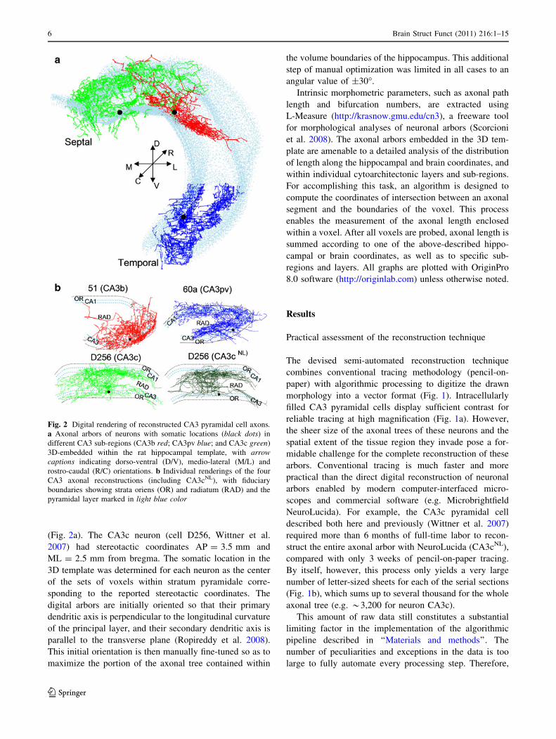
Fig. 2 Digital rendering of reconstructed CA3 pyramidal cell axons.a Axonal arbors of neurons with somatic locations (black dots) in

different CA3 sub-regions (CA3b red; CA3pv blue; and CA3c green)

3D-embedded within the rat hippocampal template, with arrowcaptions indicating dorso-ventral (D/V), medio-lateral (M/L) and

rostro-caudal (R/C) orientations. b Individual renderings of the four

CA3 axonal reconstructions (including CA3cNL), with fiduciary

boundaries showing strata oriens (OR) and radiatum (RAD) and the

pyramidal layer marked in light blue color

6 Brain Struct Funct (2011) 216:1–15

123

although the actual computing time is relatively negligible,

the sheer execution of the procedure leading from the

manual tracings to the digital reconstruction requires

almost as much time as the drawing itself. Moreover, the

product of this procedure still requires considerable human

intervention to ensure rigorous quality control. In particu-

lar, partial 2D projections of the digital reconstruction must

be checked against the corresponding tiled images. Once

again, although this operation is not unique or even

uncommon, the exquisite number of sections and size of

each makes this necessary step notably time consuming.

More specifically, quality checks and related corrections

and adjustments cost in our hands approximately the same

amount of time as each of the previous two aspects (manual

tracing and execution of the algorithm pipeline).

As a result, the full reconstruction of complete CA3

pyramidal cell axons from mounted slides to finalized

digital files is estimated to take approximately 9 weeks of

full-time skilled labor per neuron with this technique. This

is a definitive improvement compared with the 6 months

required by existing state-of-the-art solutions, and enabled

the first quantitative comparative analysis of three axonal

morphologies, which is described below.

3D appearance and intrinsic morphometry of CA3

pyramidal cell axons

The digital reconstructions of the traced neurons were

embedded in the hippocampal 3D template (Fig. 2) as

described in ‘‘Materials and methods’’. The three somata

were located in area CA3c near the septal pole (cell D256

in Wittner et al. 2007), area CA3b towards the middle of

the longitudinal axis (cell 51 in Li et al. 1994), and area

posterior/ventral or CA3pv near the temporal pole (cell 60

in Figs. 1, 2, and 12 of Li et al. 1994; cell 60a in Turner

et al. 1995), respectively (Fig. 2a). Each of the three neu-

rons displayed a uniquely distinct arbor shape. The digital

reconstruction previously acquired with the standard Neu-

roLucida system by a different operator (CA3cNL) was

recognizably similar to the morphology traced from the

same slides with the present system (Fig. 2b). In each of

the three neurons, the axonal extent spanned a sizeable

proportion of the whole hippocampus (Fig. 2a), far

exceeding the reach of the same neuron’s dendrites. The

ratios between total dendritic and axonal lengths were 1:13

(CA3b), 1:22 (CA3pv), and 1:27 (CA3c). The CA3c neu-

ron had the longest axonal branching (nearly half-a-meter),

and this value differed \0.5% from that of CA3cNL.

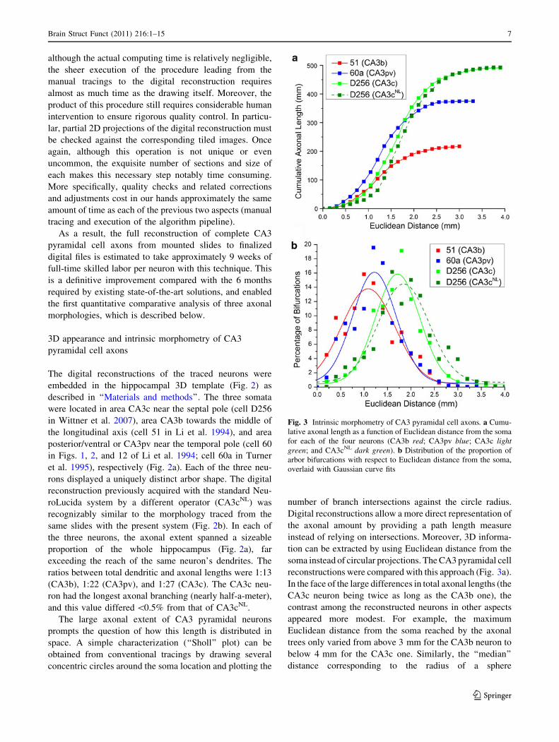
The large axonal extent of CA3 pyramidal neurons

prompts the question of how this length is distributed in

space. A simple characterization (‘‘Sholl’’ plot) can be

obtained from conventional tracings by drawing several

concentric circles around the soma location and plotting the

number of branch intersections against the circle radius.

Digital reconstructions allow a more direct representation of

the axonal amount by providing a path length measure

instead of relying on intersections. Moreover, 3D informa-

tion can be extracted by using Euclidean distance from the

soma instead of circular projections. The CA3 pyramidal cell

reconstructions were compared with this approach (Fig. 3a).

In the face of the large differences in total axonal lengths (the

CA3c neuron being twice as long as the CA3b one), the

contrast among the reconstructed neurons in other aspects

appeared more modest. For example, the maximum

Euclidean distance from the soma reached by the axonal

trees only varied from above 3 mm for the CA3b neuron to

below 4 mm for the CA3c one. Similarly, the ‘‘median’’

distance corresponding to the radius of a sphere

Fig. 3 Intrinsic morphometry of CA3 pyramidal cell axons. a Cumu-

lative axonal length as a function of Euclidean distance from the soma

for each of the four neurons (CA3b red; CA3pv blue; CA3c lightgreen; and CA3cNL dark green). b Distribution of the proportion of

arbor bifurcations with respect to Euclidean distance from the soma,

overlaid with Gaussian curve fits

Brain Struct Funct (2011) 216:1–15 7

123

encompassing 50% of the whole axonal extension was 1.3

and 1.7 mm, respectively, for the same two neurons. Both

maximum and median distances, but not total length, were

also very similar between the CA3b and CA3pv neurons.

An alternative variation of Sholl plots analyses the

proportion of bifurcation points as a function of the 3D

distance from the soma (Fig. 3b), providing an indication

of tree complexity. These measures fall at similar distances

from the soma for the CA3b and CA3pv neurons (1.1 and

1.2 mm, respectively), but farther for the CA3c cell

(1.7 mm). The spread of these distributions (computed as

standard deviation) is essentially identical for all cells,

tightly ranging from 1 to 1.1 mm. Similarly, the peak

values of these distributions are also constrained within a

narrow span between 13.4% (CA3b), and 15.6% (CA3pv).

Moreover, the measures of all of these parameters for the

CA3c neuron differ by\5% from the corresponding values

of CA3cNL, suggesting that these summary metrics of

digital reconstructions of the same neuron are reproducible

across tracing techniques and operators.

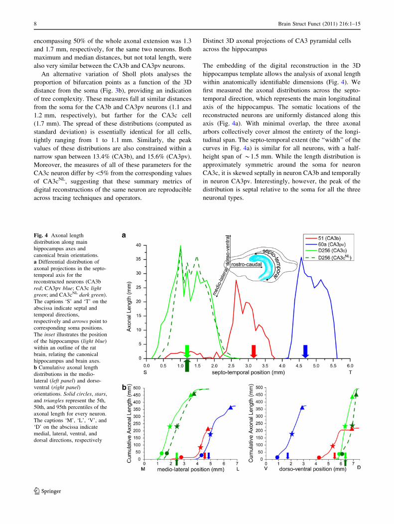
Distinct 3D axonal projections of CA3 pyramidal cells

across the hippocampus

The embedding of the digital reconstruction in the 3D

hippocampus template allows the analysis of axonal length

within anatomically identifiable dimensions (Fig. 4). We

first measured the axonal distributions across the septo-

temporal direction, which represents the main longitudinal

axis of the hippocampus. The somatic locations of the

reconstructed neurons are uniformly distanced along this

axis (Fig. 4a). With minimal overlap, the three axonal

arbors collectively cover almost the entirety of the longi-

tudinal span. The septo-temporal extent (the ‘‘width’’ of the

curves in Fig. 4a) is similar for all neurons, with a half-

height span of *1.5 mm. While the length distribution is

approximately symmetric around the soma for neuron

CA3c, it is skewed septally in neuron CA3b and temporally

in neuron CA3pv. Interestingly, however, the peak of the

distribution is septal relative to the soma for all the three

neuronal types.

Fig. 4 Axonal length

distribution along main

hippocampus axes and

canonical brain orientations.a Differential distribution of

axonal projections in the septo-

temporal axis for the

reconstructed neurons (CA3b

red; CA3pv blue; CA3c lightgreen; and CA3cNL dark green).

The captions ‘S’ and ‘T’ on the

abscissa indicate septal and

temporal directions,

respectively and arrows point to

corresponding soma positions.

The inset illustrates the position

of the hippocampus (light blue)

within an outline of the rat

brain, relating the canonical

hippocampus and brain axes.

b Cumulative axonal length

distributions in the medio-

lateral (left panel) and dorso-

ventral (right panel)orientations. Solid circles, stars,

and triangles represent the 5th,

50th, and 95th percentiles of the

axonal length for every neuron.

The captions ‘M’, ‘L’, ‘V’, and

‘D’ on the abscissa indicate

medial, lateral, ventral, and

dorsal directions, respectively

8 Brain Struct Funct (2011) 216:1–15

123

Next, we examined the axonal projections against the

canonical brain axes most univocally relevant to the hip-

pocampal orientation, namely dorso-ventral and medio-

lateral, corresponding to horizontal and sagittal planes,

respectively (Fig. 4b). In the dorso-ventral direction, the

axonal span differs substantially among the CA3 pyramidal

cells. This is evident from the position at which each of

these axonal arbors crosses the 5th, 50th, and 95th length

percentiles (Fig. 4b, left panel). For the CA3c neuron, 90%

of the total axonal length falls within less than a millimeter.

For the CA3b neuron, the same relative span is nearly three

times broader ([2.5 mm). A similar trend is observed in

the medio-lateral direction (Fig. 4b, right panel). In all

cases, the median position falls close to the soma.

Similar to the intrinsic morphometrics, the two digital

morphologies traced from the same neuron by independent

operators and with different reconstruction systems (CA3c

and CA3cNL) have comparable length distributions relative

both to the hippocampus (Fig. 4a) and brain (Fig. 4b) axes.

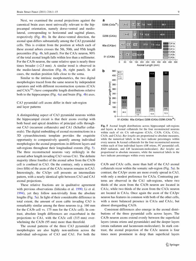
CA3 pyramidal cell axons differ in their sub-region

and layer patterns

A distinguishing aspect of CA3 pyramidal neurons within

the hippocampal circuit is that their axons overlap with

both basal and apical dendrites of principal cells through-

out CA3 (recurrent collaterals) and CA1 (Schaffer collat-

erals). The digital embedding of axonal reconstructions in a

3D cytoarchitectonic template provides the exquisite

opportunity to comparatively quantify among individual

morphologies the axonal proportions in different layers and

sub-regions throughout their longitudinal extents (Fig. 5).

The three reconstructed neurons vary strikingly in the

axonal arbor length invading CA3 versus CA1. The definite

majority (three fourths) of the axonal arbor from the CA3b

cell is confined in CA3. On the contrary, only a minority

(two fifth) of the axon of the CA3c neuron remains in CA3.

Interestingly, the CA3pv cell presents an intermediate

pattern, with a nearly identical split between CA3 and CA1

axonal projections.

These relative fractions are in qualitative agreement

with previous observations (Ishizuka et al. 1990; Li et al.

1994), yet they follow non-trivially from the absolute

lengths (Fig. 5a). In light of their considerable difference in

total extent, the amount of axon cable invading CA3 is

remarkably similar among the three neurons (e.g. 160 mm

for the CA3b cell vs. 175 mm for the CA3c cell). In con-

trast, absolute length differences are exacerbated in the

projections to CA1, with the CA3c cell (315 mm) over-

whelming the CA3b (95 mm) more than threefold.

The axonal patterns of the three CA3 pyramidal cell

morphologies are also highly non-uniform across the

individual sub-regions of CA3 and CA1. For both the

CA3b and CA3c cells, more than half of the CA3 axonal

collaterals recur within the somatic sub-region (Fig. 5a). In

contrast, the CA3pv axons are more evenly spread in CA3,

with only a modest preference for CA3a. Contrasting pat-

terns are observed in the CA1 sub-regions, where two

thirds of the axon from the CA3b neuron are located in

CA1c, while two thirds of the axon from the CA3c neuron

are located in CA1a. Once again the axon of the CA3pv

neuron has features in common with both of the other cells,

with a more balanced presence in CA1a and CA1c, but

almost disregarding CA1b.

Consistent differences also emerge in the axonal distri-

butions of the three pyramidal cells across layers. The

CA3b neuron axons extend evenly between the superficial

layers (strata oriens and pyramidale) and the deeper layers

(strata radiatum and lacunosum-moleculare). In stark con-

trast, the axonal projection of the CA3c neuron is four

times more prominent in deep than superficial layers

Fig. 5 Axonal length distributions across hippocampal sub-regions

and layers. a Axonal collaterals for the four reconstructed neurons

within each of six CA sub-regions (CA3c, CA3b, CA3a, CA1c,

CA1b, and CA1a). Bar lengths are proportional to absolute measures,

while the numerical labels in the bars indicate percentages within

every neuron. b Axonal collaterals for the four reconstructed neurons

within each of four individual layers (OR oriens, PC pyramidal cell,

RAD radiatum, and LM lacunosum-moleculare). Bar heights are

proportional to absolute measures, while the numerical labels in the

bars indicate percentages within every neuron

Brain Struct Funct (2011) 216:1–15 9

123

(Fig. 5b). As a reoccurring theme, the deep/superficial ratio

is intermediate for the CA3pv neuron. Similar to the

observation regarding the sub-regional patterns, these rel-

ative proportions reflect opposing absolute distributions.

The total axonal length in the superficial layers is nearly

the same for the three CA3 pyramidal cells (just above

100 mm), whilst the axonal presence of the CA3c neuron

in the deep CA layers is more than three times that of the

CA3b cell. Also as in the other analyses, both absolute and

relative axonal values appear to be robust between the

CA3c and CA3NL reconstructions both across layers and

sub-regions (Fig. 5).

The approximately 10% of axonal length found in the

pyramidal layer may appear surprising since these fibers do

not form synapses on somata. A possible explanation for

this finding is that digital reconstructions do not differen-

tiate explicitly main axons from axon collaterals with

boutons. We measured the mean axonal diameter in the

pyramidal versus non-pyramidal layer, and we found no

differences in any of the cells. Thus, the portions of the

axons in the pyramidal cell layer are not thicker than

the average branches. Another possibility is that axons in

the pyramidal layer contact dendrites on the basal arbor of

superficial neurons and apical arbors of deeper neurons.

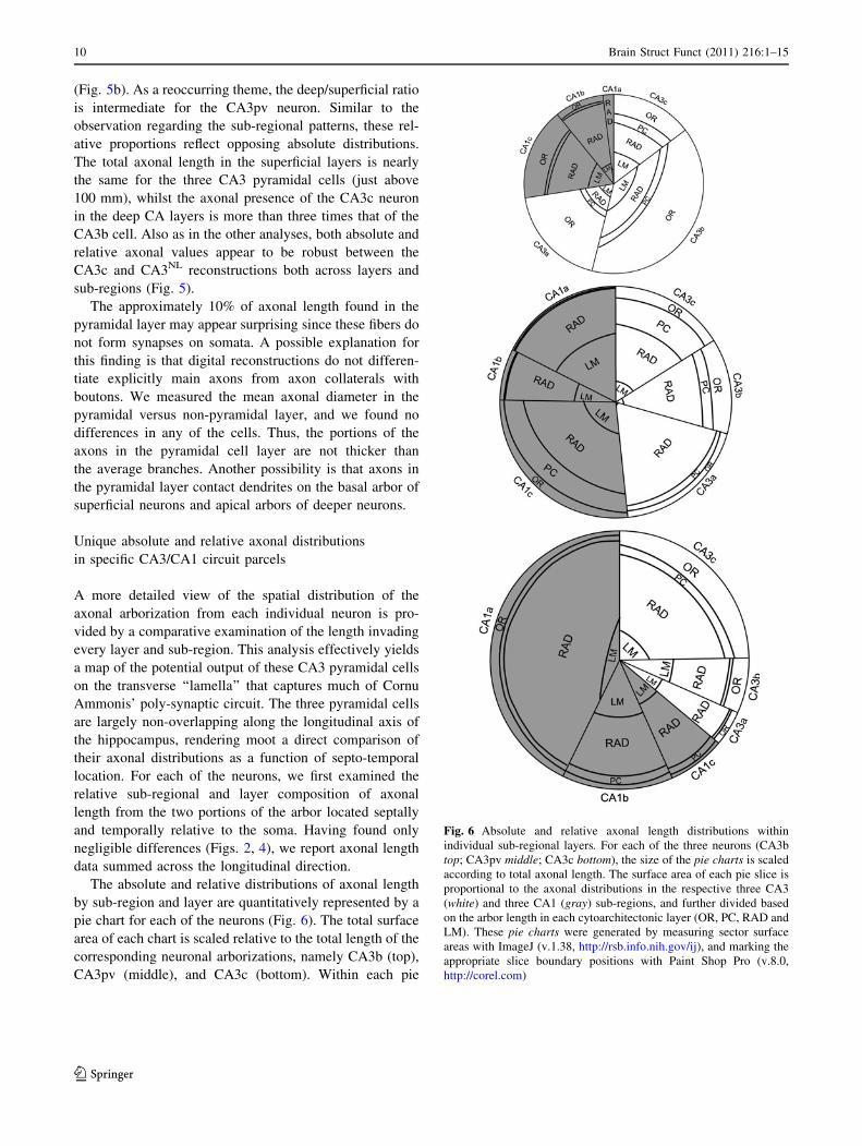
Unique absolute and relative axonal distributions

in specific CA3/CA1 circuit parcels

A more detailed view of the spatial distribution of the

axonal arborization from each individual neuron is pro-

vided by a comparative examination of the length invading

every layer and sub-region. This analysis effectively yields

a map of the potential output of these CA3 pyramidal cells

on the transverse ‘‘lamella’’ that captures much of Cornu

Ammonis’ poly-synaptic circuit. The three pyramidal cells

are largely non-overlapping along the longitudinal axis of

the hippocampus, rendering moot a direct comparison of

their axonal distributions as a function of septo-temporal

location. For each of the neurons, we first examined the

relative sub-regional and layer composition of axonal

length from the two portions of the arbor located septally

and temporally relative to the soma. Having found only

negligible differences (Figs. 2, 4), we report axonal length

data summed across the longitudinal direction.

The absolute and relative distributions of axonal length

by sub-region and layer are quantitatively represented by a

pie chart for each of the neurons (Fig. 6). The total surface

area of each chart is scaled relative to the total length of the

corresponding neuronal arborizations, namely CA3b (top),

CA3pv (middle), and CA3c (bottom). Within each pie

Fig. 6 Absolute and relative axonal length distributions within

individual sub-regional layers. For each of the three neurons (CA3b

top; CA3pv middle; CA3c bottom), the size of the pie charts is scaled

according to total axonal length. The surface area of each pie slice is

proportional to the axonal distributions in the respective three CA3

(white) and three CA1 (gray) sub-regions, and further divided based

on the arbor length in each cytoarchitectonic layer (OR, PC, RAD and

LM). These pie charts were generated by measuring sector surface

areas with ImageJ (v.1.38, http://rsb.info.nih.gov/ij), and marking the

appropriate slice boundary positions with Paint Shop Pro (v.8.0,

http://corel.com)

10 Brain Struct Funct (2011) 216:1–15

123

chart, every slice has a surface area proportional to the

axonal length in each of the three CA3 (white background)

and three CA1 (gray background) sub-regions. All slices

are further divided into four sectors with surface areas

sized according to the represented cytoarchitectonic layers

(from outermost to innermost: strata oriens, pyramidale,

radiatum, and lacunosum-moleculare). Therefore, the

ensemble view of the pie charts enables a relative assess-

ment of the axonal composition among neurons, sub-

regions, and layers. At the same time, the surface area of

each of the slice sectors (and any of their combinations)

constitutes a measure of the actual axonal length of the

given cell in the corresponding hippocampal sub-region

and layer, thus allowing absolute comparisons.

The axonal distributions among sub-regional layers

follow the same general trends reported separately for the

sub-regional compositions summed across layers and the

layer compositions summed across sub-regions reported in

Fig. 5. However, this more detailed analysis additionally

reveals specific differences, which are most extreme

between the CA3b and the CA3c cells. In the CA3b neu-

ron, the oriens layer in CA3b alone accounts for nearly

one-fifth (18%) of the entire axonal extent, compared, e.g.,

with a meager 2% in the radiatum layer of CA1a. In con-

trast, almost one-third of the whole axon of the CA3c

neuron (32%) is found in the CA1a radiatum layer, as

opposed to a negligible presence (\2%) in the CA3b oriens

layer. Interestingly, the CA3b cell extends more oriens than

radiatum axonal length in CA3, but more radiatum than

oriens in CA1.

The differences between the CA3c and CA3b cells are

somewhat blended in the CA3pv neuron, where stratum

radiatum has a uniform axonal majority in all six CA sub-

regions. Interesting trends are also shared among all three

reconstructed neurons. In all cases, for example, the axonal

length ratio between oriens and radiatum is greater in CA3

than in CA1 and, within CA1, increases moving transver-

sally from the subicular end toward CA3 (CA1a–CA1c). In

other words, there is more axon in radiatum than in oriens

in both CA1 and CA3, but the proportion of the total that is

in oriens is greater in CA1 and increases from the subic-

ulum end of CA1 to the CA2 border.

The substantial differences in total axonal length among

the three neurons yield a different perspective when com-

paring axonal distributions throughout the sub-regional

layers in absolute, rather than relative, terms. For instance,

the absolute axonal length of the CA3b neuron invading the

oriens layer of area CA3b (39.3 mm) is very similar to the

amount of CA3c axon invading the radiatum layer of area

CA1b (41.3 mm), even if they constitute very different

fractions of their respective arbors (18 vs. 8.4%, respec-

tively). In contrast, the same 8.4% fraction of the CA3b

neuron occupying the oriens layer of area CA3a only

amounts to a length of 18.4 mm. Likewise, the axonal

length of the CA3b neuron found in the radiatum layer of

area CA3b (26.2 mm) closely matches the value for the

CA3c neuron in the radiatum layer of area CA1c

(25.5 mm), while their relative proportions are more than

twofold off (12 vs. 5.2%). A similar 5.1% proportion of the

CA3b neuron invading the radiatum layer of area CA3c

corresponds to an absolute length of just 11 mm.

In some cases, the absolute size differences among

neurons accentuate, rather than compensate, the non-uni-

form relative distributions across sub-regional layers. For

example, in terms of absolute length, stratum radiatum of

area CA1a receives 36 times more axon from the CA3c

neuron than from the CA3b neuron (156 vs. 4.3 mm).

These observations were qualitatively confirmed post-hoc

by direct microscopic inspection of the slices. For example,

inspection of the CA3b neuron slide revealed very sparse

axonal presence in the radiatum layer of area CA1a, while

the same region of interest displayed dense axonal labeling

in the CA3c neuron slide.

Discussion

Axonal morphology sculpts network connectivity (Stepa-

nyants and Chklovskii 2005; Stepanyants et al. 2008) and

intrinsic neuronal processing (Manor et al. 1991; Debanne

2004). Thus, its quantitative characterization is crucial to

understand structure–function relationship in the brain.

Modern computer-interfaced microscopes and commercial

software (e.g. NeuroLucida) allow the direct reconstruction

of imaged neuronal arbors into digital format (Ascoli

2006). In practice, however, the ergonomics of the human–

equipment interaction typically restrict this possibility to

neurites of limited extent, such as dendritic trees or local

axons. Larger projections, like axons of principal cells in

the mammalian cortex, are more commonly only traced

‘‘pencil-on-paper’’ by simple Camera Lucida technique.

Unfortunately, the resulting analog drawings are less con-

ducive to quantitative analysis.

In this work, we extended a semi-automated approach

for digitally reconstructing neuronal arbors all the way

back to the initial step of basic Camera Lucida, allowing

the first quantitative analysis of multiple CA3 pyramidal

cell axons intracellularly labeled in vivo. Evaluating

intrinsic cell-to-cell variability beyond single neuron

samples from each of distinct area (CA3c, CA3b, and

CA3pv) will require even greater automation (Ascoli

2008). At the same time, full axonal arbors are dozens of

times larger than typical dendritic trees, making these

reconstructions remarkably data-rich. Previous studies

proved even individual axon reconstructions to be deeply

informative (e.g. Sik et al. 1993; Tamamaki et al. 1988).

Brain Struct Funct (2011) 216:1–15 11

123

Here, we used the only one of these previously acquired

data files that is independently available in digital format

(Wittner et al. 2007) to validate our novel semi-automated

digitization system by reconstructing the same cell from

the same slides. All morphometric measures employed in

this report showed excellent consistency between these two

data files.

To appreciate the massiveness of these axonal tracings it

is useful to compare these morphologies with other digital

reconstructions available from NeuroMorpho.Org, the

largest available collection of neuronal tracings (Ascoli

et al. 2007), and relevant hippocampal literature. A dentate

gyrus granule cell filled in vivo has total axonal lengths of

approximately 9 mm (Scorcioni and Ascoli 2005), which is

only *3 times that of the dendritic arborization for the

same cell type (e.g. Claiborne et al. 1990). Hippocampal

interneurons from CA3b strata radiatum and lacunosum-

moleculare have typical axonal and dendritic lengths of

*20 and *3 mm, respectively (Ascoli et al. 2009), but

their completeness cannot be established conclusively

since these were injected in slices. One of the interneuron

described from the dentate gyrus had very extensive axonal

arbor, potentially comparable to that of pyramidal cells

(Sik et al. 1997). Although not fully reconstructed, long-

range interneurons also have very dense axons (Sik et al.

1994). Because of their substantially larger axon caliber

(Jinno et al. 2007) the total axonal volume of these long-

range interneurons can be several times larger than that of

pyramidal cells.

At the same time, other principal neurons from the

mammalian cerebral cortex in NeuroMorpho.Org have

axonal length of the same order of magnitude as the values

reported here, such as a pyramidal cell from the visual

cortex of the cat at *110 mm even if incomplete (Hirsch

et al. 2002), a spiny stellate cell from the entorhinal cortex

of the rat at *160 mm without including full local col-

laterals (Tamamaki and Nojyo 1995), and a CA2 pyramidal

cell from the rat hippocampus at *430 mm (Tamamaki

et al. 1988). Except for the cat visual cortex example, all

these other principal cell axonal reconstructions were

obtained with the previous version of the semi-automated

reconstruction technique employed here (Scorcioni and

Ascoli 2005). In sharp contrast, axons traced from cells

intracellularly filled in the slice have much more contained

axonal length most probably due to axotomy. For example,

pyramidal cells from monkey prefrontal cortex have total

axonal length of *35 mm (Gonzalez-Burgos et al. 2004).

Therefore, in terms of data density, the three CA3 pyra-

midal cell axonal reconstructions described here and pub-

licly distributed at NeuroMorpho.Org contribute great

potential for subsequent analysis and modeling.

The ipsilateral axonal projections of CA3 pyramidal

neurons generate two crucial associational pathways in the

neurobiology of learning and memory: the recurrent col-

laterals within area CA3 and the Schaffer collaterals into

area CA1. Previous studies (Ishizuka et al. 1990; Li et al.

1994) indicated that the relative balance of these two sys-

tems depends on the longitudinal and transverse location of

the presynaptic cell, as well as the targeted sub-regions

(CA3/CA1a,b,c) and layers (oriens/radiatum). By embed-

ding three digitally reconstructed axons within a 3D tem-

plate of the rat hippocampus, our approach quantified

specific patterns of axonal collaterals throughout every

cytoarchitectonic location along the septo-temporal axis.

In dorsal hippocampus, dramatic quantitative differ-

ences were measured between CA3c and CA3b pyramidal

cells. The CA3c neuron projected twice as much axon to

CA1 as to CA3, and, within CA1, twice as much in CA1a

(distally) than in CA1b and CA1c combined. Throughout

these regions, this axonal arbor overwhelmingly preferred

stratum radiatum to oriens by a 6:1 ratio. In contrast, the

CA3b neuron projected thrice as much axon to CA3 than to

CA1, and, within CA3, 50% more to CA3b (locally) than to

CA3a and CA3c combined. Within CA1, this neuron

extended 50% more length in CA1c (proximally) than in

CA1a and CA1b combined. While within CA3b the

recurrent collateral preferred stratum oriens to radiatum by

50% margin, the trend was reversed in the Schaffer pro-

jections to CA1, where radiatum trumped oriens 3:1.

Such diametrical opposition suggests a possible sub-

regional and cytoarchitectonic specialization for the dual

organization of CA3 axons into recurrent and Schaffer

collaterals, as also reflected by physiological studies

(Csicsvari et al. 2000, 2003). Distal projections to CA1

predominate in CA3c and preferentially target the radiatum

layer. Local arbors predominate in CA3b and preferentially

target the oriens layer. This putative division could in turn

hint to an alteration of the classic view of the hippocampal

synaptic circuit. Rather than region uniform receiving en-

torhinal input (directly and through the dentate gyrus) and

transmitting output to CA1, area CA3 might be serially

composed of a first station (CA3b) suitable to receive and

locally distribute input within CA3, followed by a second

station (CA3c) mainly dedicated to propagate the output

downstream to CA1. This alternative view is also sup-

ported by prominent dendritic branching ([15% of total

dendritic length) of CA3b pyramidal cells in stratum

lacunosum-moleculare (the layer invaded by the entorhinal

perforant pathway) compared with almost negligible den-

dritic presence (\3% of total dendritic length) of CA3c

neurons in this layer (Ishizuka et al. 1995).

The opposite trends observed in CA3c and CA3b neu-

rons from the dorsal hippocampus are somewhat blended in

the pyramidal cells reconstructed from the posterior/ventral

area, with axonal collaterals more uniformly distributed

throughout all sub-regions. The substantial differences in

12 Brain Struct Funct (2011) 216:1–15

123

total arbor length among the reconstructed neurons com-

bine with their relative differences in sub-region and layer

distributions, resulting in relative constant absolute values

of axonal extent, e.g. in the combined oriens and pyramidal

layers (very close to 100 mm for all three cells) or within

sub-regions CA3a,b,c together (*170 mm for all three

cells). Thus, pyramidal cell output might be specifically

differentiated for selective targets (CA1 and radiatum), yet

relatively stable for others.

Recent studies reported CA3 back-projections to the

dentate gyrus (Scharfman 2007), especially towards the

temporal pole (Witter 2007). Also at least one neuron

described in the ventral hippocampus (cell r32 in Li et al.

1994) extensively collateralized in the dentate molecular

layer. For each of our three neurons, the axonal length within

the hilus fell within the margin of measurement error

(2–2.5%) and was neglected. Another open question not

tackled by the present study regards the relative extent of the

commissural projection to the controlateral hippocampus.

Functionally, the CA3 region is recognized to play

important roles in memory encoding and retrieval (Treves

and Rolls 1994; Treves 2004; Kunec et al. 2005). In most

physiological, behavioral, and computational studies, CA3 is

considered a single functional region. Recently, however,

lesion studies in the rat showed dissociation between CA3

sub-regions (Hunsaker et al. 2008). Specifically, CA3c

lesions yielded greater spatial deficits than lesions in sub-

regions CA3a and CA3b. These sub-regions are also differ-

entially involved in initiating and transferring population

patterns (Csicsvari et al. 2000). Such functional specializa-

tion of individual CA3 sub-regions (Kesner 2007) is con-

sistent with the differential axonal collateral patterns of

CA3c and CA3b pyramidal cells demonstrated here.

Lesion studies also revealed dorso-ventral functional

differentiation (Bannerman et al. 1999; Hock and Bunsey

1998; Hunsaker and Kesner 2008), whereas dorsal, but not

ventral, rat hippocampus appears involved in spatial

behavior, as also supported by physiological observations

(Royer et al. 2010). Differing circuit organizations might

underlie the functional dissociation of dorsal and ventral

hippocampus (Moser and Moser 1998). Among the neurons

we reconstructed, the posterior/ventral pyramidal cell dis-

played an axonal distribution pattern intermediate between

those of CA3c and CA3b neurons in dorsal hippocampus.

This might indicate a less distinct sub-regional differenti-

ation in ventral than in dorsal hippocampus, consistent as

well with the relatively more uniform axonal distribution of

the CA3pv cell among individual cytoarchitectonic layers

throughout the six CA3/CA1 areas.

Axonal reconstructions can be utilized to estimate

potential synaptic connectivity patterns based on geometri-

cal overlaps with dendritic arbors (Stepanyants et al. 2002;

Kalisman et al. 2003). While thousands of digital dendritic

reconstructions are readily available in the public domain

(Ascoli et al. 2007), no axons have been fully traced for most

known neuron classes. The free distribution of the digital

morphologies described here through the NeuroMorpho.Org

database should thus constitute a useful addition to shared

neuroscience resources. Axonal territory provides a map of

necessary, but not sufficient conditions to characterize syn-

aptic connectivity, as individual synapses might abide spe-

cific, localized, and compartmentalized criteria (Shepherd

and Harris 1998). In the hippocampus, however, axo-den-

dritic overlap predicts actual contacts in at least some neuron

types (Stepanyants et al. 2004). In the heydays of con-

nectomics (Kennedy 2010), the key information about net-

works is quantitative neuronal connectivity in vivo.

Complete axonal arbors of single neurons are still unsolvable

with any of the ongoing connectomics approaches due to

limits of resolution (non-invasive imaging), sampling

(fluorescent genetic labeling) or field-of-view (electron

microscopy). Although time-consuming, intracellular

labeling is critical to elucidate connections between neuron

types.

Axonal signal propagation also depends on the geometry

of its arbor. The intrinsic axonal length properties of CA3

pyramidal cells could affect action potential conduction

velocity and even branch point failure in these complex 3D

arbors. These effects might influence spike timing and

delays, therefore imposing noteworthy computational

constraints on temporal coding (Carr and Konishi 1990;

McAlpine and Grothe 2003). Although we are still at the

beginning of the path towards understanding how the

functions of the nervous system emerge from the structure

and activity of its circuit, this study represents a step for-

ward in elucidating the morphological organization of one

of the most plastic networks in the adult mammalian brain.

Acknowledgments We are indebted to Todd Gillette and Maryam

Halavi for their valuable feedback on an earlier version of this manu-

script, to Aruna Muthulu for scanning and aligning the tracings, and to

Lucia Wittner for sharing reconstruction CA3cNL on NeuroMorpho.Org.

Grant sponsor: National Institute of Health Grant numbers: NS39600 &

NS058816 to GAA, and NS34994 & MH54671 to GB.

References

Ascoli GA (2006) Mobilizing the base of neuroscience data: the case

of neuronal morphologies. Nat Rev Neurosci 7:318–324

Ascoli GA (2008) Neuroinformatics grand challenges. Neuroinfor-

matics 6:1–3

Ascoli GA, Donohue DE, Halavi M (2007) NeuroMorpho.Org: a

central resource for neuronal morphologies. J Neurosci

27:9247–9251

Ascoli GA, Brown KM, Calixto E, Card JP, Galvan EJ, Perez-Rosello

T, Barrionuevo G (2009) Quantitative morphometry of electro-

physiologically identified CA3b interneurons reveals robust local

geometry and distinct cell classes. J Comp Neurol 515:677–695

Brain Struct Funct (2011) 216:1–15 13

123

Bannerman DM, Yee BK, Good MA, Heupel MJ, Iversen SD,

Rawlins JN (1999) Double dissociation of function within the

hippocampus: a comparison of dorsal, ventral, and complete

hippocampal cytotoxic lesions. Behav Neurosci 113:1170–1188

Buzsaki G (1986) Hippocampal sharp waves: their origin and

significance. Brain Res 398:242–252

Carr CE, Konishi M (1990) A circuit for detection of interaural time

differences in the brain stem of the barn owl. J Neurosci

10:3227–3246

Claiborne BJ, Amaral DG, Cowan WM (1990) Quantitative, three-

dimensional analysis of granule cell dendrites in the rat dentate

gyrus. J Comp Neurol 302:206–219

Csicsvari J, Hirase H, Mamiya A, Buzsaki G (2000) Ensemble

patterns of hippocampal CA3-CA1 neurons during sharp wave-

associated population events. Neuron 28:585–594

Csicsvari J, Jamieson B, Wise KD, Buzsaki G (2003) Mechanisms of

gamma oscillations in the hippocampus of the behaving rat.

Neuron 37:311–322

Debanne D (2004) Information processing in the axon. Nat Rev

Neurosci 5:304–316

Gonzalez-Burgos G, Krimer LS, Urban NN, Barrionuevo G, Lewis

DA (2004) Synaptic efficacy during repetitive activation of

excitatory inputs in primate dorsolateral prefrontal cortex. Cereb

Cortex 14:530–542

Hirsch JA, Martinez LM, Alonso JM, Desai K, Pillai C, Pierre C

(2002) Synaptic physiology of the flow of information in the

cat’s visual cortex in vivo. J Physiol 540:335–350

Hock BJ Jr, Bunsey MD (1998) Differential effects of dorsal and

ventral hippocampal lesions. J Neurosci 18:7027–7032

Hunsaker MR, Kesner RP (2008) Dissociations across the dorsal-

ventral axis of CA3 and CA1 for encoding and retrieval of

contextual and auditory-cued fear. Neurobiol Learn Mem

89:61–69

Hunsaker MR, Rosenberg JS, Kesner RP (2008) The role of the

dentate gyrus, CA3a, b, and CA3c for detecting spatial and

environmental novelty. Hippocampus 18:1064–1073

Ishizuka N, Weber J, Amaral DG (1990) Organization of intrahip-

pocampal projections originating from CA3 pyramidal cells in

the rat. J Comp Neurol 295:580–623

Ishizuka N, Cowan WM, Amaral DG (1995) A quantitative analysis

of the dendritic organization of pyramidal cells in the rat

hippocampus. J Comp Neurol 362:17–45

Jinno S, Klausberger T, Marton LF, Dalezios Y, Roberts JD,

Fuentealba P, Bushong EA, Henze D, Buzsaki G, Somogyi P

(2007) Neuronal diversity in GABAergic long-range projections

from the hippocampus. J Neurosci 27:8790–8804

Kalisman N, Silberberg G, Markram H (2003) Deriving physical

connectivity from neuronal morphology. Biol Cybern 88:210–

218

Kennedy DN (2010) Making connections in the connectome era.

Neuroinformatics 8:61–62

Kesner RP (2007) Behavioral functions of the CA3 subregion of the

hippocampus. Learn Mem 14:771–781

Kunec S, Hasselmo ME, Kopell N (2005) Encoding and retrieval in

the CA3 region of the hippocampus: a model of theta-phase

separation. J Neurophysiol 94:70–82

Li XG, Somogyi P, Ylinen A, Buzsaki G (1994) The hippocampal

CA3 network: an in vivo intracellular labeling study. J Comp

Neurol 339:181–208

Lorente de No R (1934) Studies on the structure of the cerebral cortex

II. Continuation of the study of the ammonic system. J Psychol

Neurol 46:113–117

Manor Y, Koch C, Segev I (1991) Effect of geometrical irregularities

on propagation delay in axonal trees. Biophys J 60:1424–1437

McAlpine D, Grothe B (2003) Sound localization and delay lines–do

mammals fit the model? Trends Neurosci 26:347–350

Moser MB, Moser EI (1998) Functional differentiation in the

hippocampus. Hippocampus 8:608–619

Pyapali GK, Sik A, Penttonen M, Buzsaki G, Turner DA (1998)

Dendritic properties of hippocampal CA1 pyramidal neurons in

the rat: intracellular staining in vivo and in vitro. J Comp Neurol

391:335–352

Ramon y Cajal S (1911) Histologie du Systeme Nerveux. Maloine,

Paris

Rolls ET (2007) An attractor network in the hippocampus: theory and

neurophysiology. Learn Mem 14:714–731

Ropireddy D, Bachus S, Scorcioni R, Ascoli GA (2008) Computa-

tional neuroanatomy of the rat hippocampus: implications and

application to epilepsy. In: Soltesz I, Staley K (eds) Computa-

tional neuroscience in epilepsy. Elsevier, San Diego, pp 71–85

Royer S, Sirota A, Patel J, Buzsaki G (2010) Distinct representations

and theta dynamics in dorsal and ventral hippocampus. J Neu-

rosci 30:1777–1787

Scharfman HE (2007) The CA3 ‘‘backprojection’’ to the dentate

gyrus. Prog Brain Res 163:627–637

Scorcioni R, Ascoli GA (2005) Algorithmic reconstruction of

complete axonal arborizations in rat hippocampal neurons.

Neurocomputing 65–66:15–22

Scorcioni R, Polavaram S, Ascoli GA (2008) L-Measure: a web-

accessible tool for the analysis, comparison and search of digital

reconstructions of neuronal morphologies. Nat Protoc 3:866–876

Shepherd GM, Harris KM (1998) Three-dimensional structure and

composition of CA3 ? CA1 axons in rat hippocampal slices:

implications for presynaptic connectivity and compartmentali-

zation. J Neurosci 18:8300–8310

Sik A, Tamamaki N, Freund TF (1993) Complete axon arborization

of a single CA3 pyramidal cell in the rat hippocampus, and its

relationship with postsynaptic parvalbumin-containing interneu-

rons. Eur J Neurosci 5:1719–1728

Sik A, Ylinen A, Penttonen M, Buzsaki G (1994) Inhibitory CA1-

CA3-hilar region feedback in the hippocampus. Science

265:1722–1724

Sik A, Penttonen M, Buzsaki G (1997) Interneurons in the

hippocampal dentate gyrus: an in vivo intracellular study. Eur

J Neurosci 9:573–588

Stepanyants A, Chklovskii DB (2005) Neurogeometry and potential

synaptic connectivity. Trends Neurosci 28:387–394

Stepanyants A, Hof PR, Chklovskii DB (2002) Geometry and

structural plasticity of synaptic connectivity. Neuron 34:275–288

Stepanyants A, Tamas G, Chklovskii DB (2004) Class-specific

features of neuronal wiring. Neuron 43:251–259

Stepanyants A, Hirsch JA, Martinez LM, Kisvarday ZF, Ferecsko AS,

Chklovskii DB (2008) Local potential connectivity in cat

primary visual cortex. Cereb Cortex 18:13–28

Tamamaki N, Nojyo Y (1995) Preservation of topography in the

connections between the subiculum, field CA1, and the entorh-

inal cortex in rats. J Comp Neurol 353:379–390

Tamamaki N, Abe K, Nojyo Y (1988) Three-dimensional analysis of

the whole axonal arbors originating from single CA2 pyramidal

neurons in the rat hippocampus with the aid of a computer

graphic technique. Brain Res 452:255–272

Treves A (2004) Computational constraints between retrieving the

past and predicting the future, and the CA3-CA1 differentiation.

Hippocampus 14:539–556

Treves A, Rolls ET (1994) Computational analysis of the role of the

hippocampus in memory. Hippocampus 4:374–391

Turner DA, Li XG, Pyapali GK, Ylinen A, Buzsaki G (1995)

Morphometric and electrical properties of reconstructed hippo-

campal CA3 neurons recorded in vivo. J Comp Neurol

356:580–594

Witter MP (2007) Intrinsic and extrinsic wiring of CA3: indications

for connectional heterogeneity. Learn Mem 14:705–713

14 Brain Struct Funct (2011) 216:1–15

123

Witter MP, Amaral DB (2004) Hippocampal formation. In: Paxinos G

(ed) The rat nervous system. Elsevier, San Diego, pp 635–704

Wittner L, Henze DA, Zaborszky L, Buzsaki G (2007) Three-

dimensional reconstruction of the axon arbor of a CA3

pyramidal cell recorded and filled in vivo. Brain Struct Funct

212:75–83

Wolf E, Birinyi A, Pomahazi S (1995) A fast 3-dimensional neuronal

tree reconstruction system that uses cubic polynomials to

estimate dendritic curvature. J Neurosci Methods 63:137–145

Brain Struct Funct (2011) 216:1–15 15

123