Average-cost pricing, increasing returns, and optimal ...
23
1 Average-cost pricing, increasing returns, and optimal output in a model with home and market production Yew-Kwang Ng Dept. of Economics, Monash University Email: [email protected] Dingsheng Zhang Dept. of Economics, Monash University Institute for Advanced Economic Studies, Wuhan University [email protected] Abstract The analysis of economies of specialization at the individual level by Yang & Shi (1992) and Yang & Ng (1993) is combined with the Dixit & Stiglitz (1977) analysis of monopolistic-competitive firms to show that, ignoring administrative costs and indirect effects (such as rent-seeking), even if both the home and the market sectors are produced under conditions of increasing returns and there are no pre- existing taxes, it is still efficient to tax the home sector to finance a subsidy on the market sector to offset the under-production of the latter due to the failure of price- taking consumers to take account of the effects of higher consumption in reducing the average costs and hence prices, through increasing returns or the publicness nature of fixed costs. Within market production, it is efficient to subsidise more the sector with a higher fixed cost, a lower elasticity of substitution between goods, and a lower degree of importance in preference which all increases the degree of increasing returns. Keywords: increasing returns, average-cost pricing, monopolistic competition, home production, optimal output, fixed costs. JEL Classifications: D43, H21, L11.
Transcript of Average-cost pricing, increasing returns, and optimal ...

1
Average-cost pricing, increasing returns, and optimal output
in a model with home and market production
Yew-Kwang Ng Dept. of Economics, Monash University
Email: [email protected]
Dingsheng Zhang
Dept. of Economics, Monash University
Institute for Advanced Economic Studies, Wuhan University
Abstract
The analysis of economies of specialization at the individual level by Yang &
Shi (1992) and Yang & Ng (1993) is combined with the Dixit & Stiglitz (1977)
analysis of monopolistic-competitive firms to show that, ignoring administrative
costs and indirect effects (such as rent-seeking), even if both the home and the market
sectors are produced under conditions of increasing returns and there are no pre-
existing taxes, it is still efficient to tax the home sector to finance a subsidy on the
market sector to offset the under-production of the latter due to the failure of price-
taking consumers to take account of the effects of higher consumption in reducing the
average costs and hence prices, through increasing returns or the publicness nature of
fixed costs. Within market production, it is efficient to subsidise more the sector with
a higher fixed cost, a lower elasticity of substitution between goods, and a lower
degree of importance in preference which all increases the degree of increasing
returns.
Keywords: increasing returns, average-cost pricing, monopolistic competition, home
production, optimal output, fixed costs.
JEL Classifications: D43, H21, L11.

2
Average-cost pricing, increasing returns, and optimal output
in a model with home and market production
The issue of increasing returns is one of those that will be raised incessantly as a neat
general solution is lacking and many different outcomes are possible. Increasing
returns are also prevalent in the real economy. Arrow (1995) explains how the
relevance of information and knowledge in production makes increasing returns
prevalent. (See also Wilson 1975, Radner & Stiglitz 1984, Arthur 1994. On empirical
evidence for increasing returns, see Ades & Glaeser 1999, Antweiler & Trefler 2002.)
Recent interest in the topic has also been considerable, as witnessed by a number of
collected volumes (Arrow, et al. 1998, Buchanan & Yoon 1994a, Heal 1999.)1 A
model much used in the analysis is one developed by Dixit & Stiglitz (1977) with
symmetrical monopolistic competitive firms with free entry and produced with a
fixed cost and a constant marginal cost. Though a special case, it reflects much of
reality as much of increasing returns may be traced to some big fixed-cost
components (a piece of land for farming, a factory for manufacturing production, a
shop for retailing, learning costs for many skilled activities, etc.) and the variable
costs (raw materials, intermediate goods purchased, stocks ordered, etc.) are largely
constant within a wide range. While this model captures much of increasing returns at
the firm level, those at the economy level arising from the economies of
specialization made possible by the division of labor are analysed by Yang & Ng
(1993). This latter framework starts from the most basic level of individual decisions
on what activities (home production, trade, employment, consumption, etc.) to
undertake to maximize utility and the interaction of the activities of individuals and
their implications on economic organization, trade, growth, etc. Though the
emergence of firms and other issues (including the choice of the variety of products;
see Yang & Shi 1992) are also analysed, the economies of specialization is taken to
be confined to the individual level. In principle, one may use this framework to
1 For a survey of the earlier literature on the economics of product variety which is related to monopolistic competition and increasing returns, see Lancaster (1990).

3
model the increasing returns at the firm level through the complicated interaction
between different individuals within the firm and their interaction with other factors
employed by the firm, but the complication involved may raise issues of
manageability. There are also models that analyse the increasing returns from
employing production methods with more intermediate goods (e.g. Ethier 1979,
Romer 1986, Buchanan & Yoon 1994b). However, there are advantages in directly
allowing for increasing returns at the firm level from the fixed-cost components as in
the Dixit-Stiglitz model. Moreover, the majority of production in most advanced
economies is undertaken by firms with increasing returns prevailing over the whole
relevant range of production, but also with individual home production still taking
place. The present paper combines the analysis of economies of specialization at the
individual level by Yang & Shi (1992) and Yang & Ng (1993) with the Dixit &
Stiglitz (1977) analysis of the market production by monopolistic-competitive firms.
(For an earlier model combining home production with market production by firms
emphasizing the role of the number of intermediate goods and different stages of
production, see Locay 1990. Here, the complications due to intermediate goods and
stages in production are ignored.) It is hoped that this combination moves a step
closer to the real economy with both home and firm/market production. The model
developed in Section 1 below could be used to analyse problems other than those
discussed in this paper.
It is shown in Section 1 that, even if both the home and the market sectors are
produced under conditions of increasing returns and there are no pre-existing taxes
(including income taxes) on the market sector, it is still efficient to tax the home
sector to finance a subsidy on the market sector to offset the under-production of the
latter. The home sector is not under-produced because the increasing returns there are
fully taken into account by the individuals/households. In the production by firms for
the market, as the output is priced at average cost and each consumer takes the price
as given, the effect of higher consumption in reducing the price through increasing
returns is not taken into account. Viewed differently, the fixed cost of production
possesses the publicness characteristic, causing under-production. However, the

4
taxation of the home sector may not be practically feasible. Section 2 allows market
production to have two sectors and shows that it is efficient to tax the sector with a
lower fixed cost, a higher elasticity of substitution between goods, and a higher
degree of importance in preference (as all these factors contribute to a lower degree
of increasing returns) and subsidize the other sector. Qualifications on the
applicability of these results in the real economy are discussed in the concluding
section.
1. A model with home and market production
1.1 The model
Consider an economy with M identical consumers. Each of them has the following
decision problem for consumption, working, and home production.
(1) Max: u = 1 1 2 21 [ ] [ ]r jr R j J
l x xβα ρ ρρ ρα β− −
∈ ∈∑ ∑ (utility function)
s.t. (1 )r r jr R j J
p x w l l∈ ∈
= − −∑ ∑ (budget constraint)
jj
l ax
c−
= (home production function)
where pr is the price of good r which are market goods, w is the price of labour, xr is
the amount of good r that is purchased from the market, R is the set of market goods,
xj is the amount of good j which is home good, lj is the amount of labour used in
producing home good j, a<1 is the fixed cost of producing a home good, c is the
marginal cost in home production, J is the set of home goods, l is leisure,
(1 )jj J
l l∈
− − ∑ is the amount of labour hired by firms, (0,1)iρ ∈ (open interval) is the
parameter of elasticity of substitution between each pair of consumption goods, α , β
are preference parameters, and u is the utility level. It is assumed that each consumer
is endowed with one unit of labour, which is the numeraire, so 1w = . Each consumer
is a price taker and her decision variables are l, lj and xr. It is assumed that the
elasticity of substitution 1/(1-ρi) > 1��RU���!� !i >0 for both i = 1, 2.

5
Denoting the number of home goods as m, by symmetry, the budget constraint can
be rewritten as follow:
(2) 1r r hr R
p x ml l∈
+ + =∑
where hl is labor used in the production of each home good.
)URP�WKH�/DJUDQJHDQ�IXQFWLRQ�/��ZKHUH� ��LV�XVHG�DV�WKH�PXOWLSOLHU��RI�WKH�DERYH�maximization problem, the first-order conditions2 are:
(3) 0r
Lx
∂ = ⇒∂
1 1 1 21 11 [ ] ( )h
r r rr R
l al x x m p
cβα ρ ρρ ρα β βα λ− −− −
∈
− =∑
(4) 0Lm
∂ = ⇒∂
1 1 211
2
[ ] ( )hr h
r R
l al x m l
cβα ρ ρρα β ββ λρ
−− −
∈
− =∑
(5) 0h
Ll
∂ = ⇒∂
1 1 21 1[ ] ( )hr
r R
l al x m c m
cβα ρ ρρα β ββ λ− − −
∈
− =∑
(6) 0Ll
∂ = ⇒∂
1 1 2(1 ) [ ] ( )hr
r R
l al x m
cβα ρ ρρα β βα β λ− −
∈
−− − =∑
(2) 0Lλ
∂ = ⇒∂
1r r hr R
p x ml l∈
+ + =∑
Using (2)-(6), we can get following solutions
(7) 21h
al ρ= −
(8) 2
2 2
(1 )(1 )
l ρ α βρ β ρ
− −= + −
(9) 2
2 2
(1 )[ (1 )]
ma
β ρρ β ρ
−=+ −
(10) 1 1
1 11 1
2
2 21
[ (1 )] ( )r n
r ss
xp p
ρρ ρ
αρ
ρ β ρ − −
=
=+ − ∑
where n is the number of market goods.
2 It may be checked that second-order conditions are satisfied.

6
Before we consider the behaviour of firms, we first get the own price elasticity
of demand for good r, using (10), we have
(11) 1
1
lnln (1 )
r
r
x np n
ρρ
∂ −=∂ −
This formula is called Yang-Heijdra formula ( Yang and heijdra, 1993).
Next, we consider the firms’ decision problems. We assume that the market
structure is monopolistic competition. Each firm produces a good under conditions of
increasing returns to scale. Because of global increasing returns to scale, only one
firm can survive in the market for a good. If there are two firms producing the same
good, one of them can always increase output to reduce price by utilizing further
economies of scale, thereby driving the other firm out of the market. Therefore, the
monopolist can manipulate the interaction between quantity and price to choose a
profit maximizing price. Free entry into each sector is however assumed. Free entry
will drive the profit of a marginal firm that has the lowest profit to zero. Any positive
profit of the marginal firm will invite a potential entrepreneur to set up a new firm to
produce a differentiated good. For a symmetric model, this condition implies zero
profit for all firms.
Assume that the production function of good r is
( ) /r rX l A b= −
so that the labor cost function of good r is
(12) r rl bX A= +
where A is the fixed cost and b the constant marginal cost. The first-order condition
for the monopolist to maximize profit with respect to output level or price implies
that
(13) [1 1/( ln ln )]r r rMR p x p MC b= + ∂ ∂ = =
where MR and MC stand for marginal revenue and marginal cost, respectively.
Inserting the expression for the own price elasticity of demand (ln ) (ln )r rx p∂ ∂ in (11)
into (13), we have
(14) 1
1
( )( 1)r
b np
nρ
ρ−=
−

7
The zero profit condition implies
(15) r r rp X bX A= +
1.2 General equilibrium and comparative statics
Since marked goods are symmetric, so we have r sX X X= = , ,r sx x x= =
,r sp p p= = , 1,2, ,r s n= " . In addition, home goods are also symmetric, so we
have j k hl l l= = , j k hx x x= = , , 1,2, ,j k m= " . The general equilibrium is given by (7)-
(10), (14), (15) and the market clearing condition Mx = X, which involve the unknowns
p, n, m, l, hl , x, X. Here, the subscripts of variables are skipped because of symmetry.
Hence, the general equilibrium values of the various variables are
(16) 1
1
( )( 1)
b np
nρ
ρ−=
−,
1
1
( 1)(1 )A n
Xbnρ
ρ−=
−,
1
1
( 1)(1 )A n
xbn M
ρρ−=
−,
2
2 2
(1 )(1 )
lρ α βρ β ρ
− −=+ −
,
21h
al
ρ=
−,
1
1
( )(1 )r
A nl
nρρ
−=−
,
2 11
2 2
(1 )[ (1 )]M
nA
αρ ρ ρρ β ρ
−= ++ −
,
2
2 2
(1 )[ (1 )]
ma
β ρρ β ρ
−=+ −
.
After obtaining explicit solutions for the general equilibrium values of the variables
as functions of the parameters, we may next examine the comparative statics by
examining the effects of a change in some parameter on the equilibrium values of the
variable, as given below:

8
(17) 2 1
2 2
(1 )0,
[ (1 )]nM A
αρ ρρ β ρ
∂ −= >∂ + −
2 12
2 2
(1 )0,
[ (1 )]n MA A
αρ ρρ β ρ
∂ −= − <∂ + −
2 1
2 2
(1 )0,
[ (1 )]n M
Aρ ρ
α ρ β ρ∂ −= >∂ + −
2 1 22
2 2
(1 )(1 )0,
[ (1 )]n M
Aαρ ρ ρ
β ρ β ρ∂ − −= − <∂ + −
2
1 2 2
1 0[ (1 )]
n MA
αρρ ρ β ρ
∂ = − <∂ + −
12
2 2 2
(1 )0
[ (1 )]n M
Aαβ ρ
ρ ρ β ρ∂ −= >∂ + −
2 22
2 2
(1 )0,
[ (1 )]m
aρ ρ
β ρ β ρ∂ −= >∂ + −
22
2 2
(1 )0,
[ (1 )]ma a
β ρρ β ρ
∂ −= − <∂ + −
22 2 2
0,[ (1 )]
ma
βρ ρ β ρ
∂ −= <∂ + −
.
The signs of the above comparative-statics results are all straightforward except that
for 1
nρ
∂∂
. It appears to be ambiguous. However, if we substitute the solution for n into
the solution for x in (16), we have the value of x as given in (18) below. Since the
denominator is positive and 1Aρ in the numerator is also positive, the remaining part
2 2 2{ [ (1 )]}M Aαρ ρ β ρ− + − in the numerator must also be positive for x to be
positive. 3 As x has to be positive for n to be meaningful, the sign of 1
nρ
∂∂
is in fact
unambiguously negative.
The comparative-statics results above may be seen to be intuitively agreeable,
though not all obvious. For example, an increase in population size M increases the 3 Economically, the size of the fixed cost of market production A must not be too large in relation to the population size M. Otherwise the economy may not be viable if the labour of all people combined is insufficient to provide for the fixed cost of production, allowing for the necessity of producing some home goods and having some leisure.
9
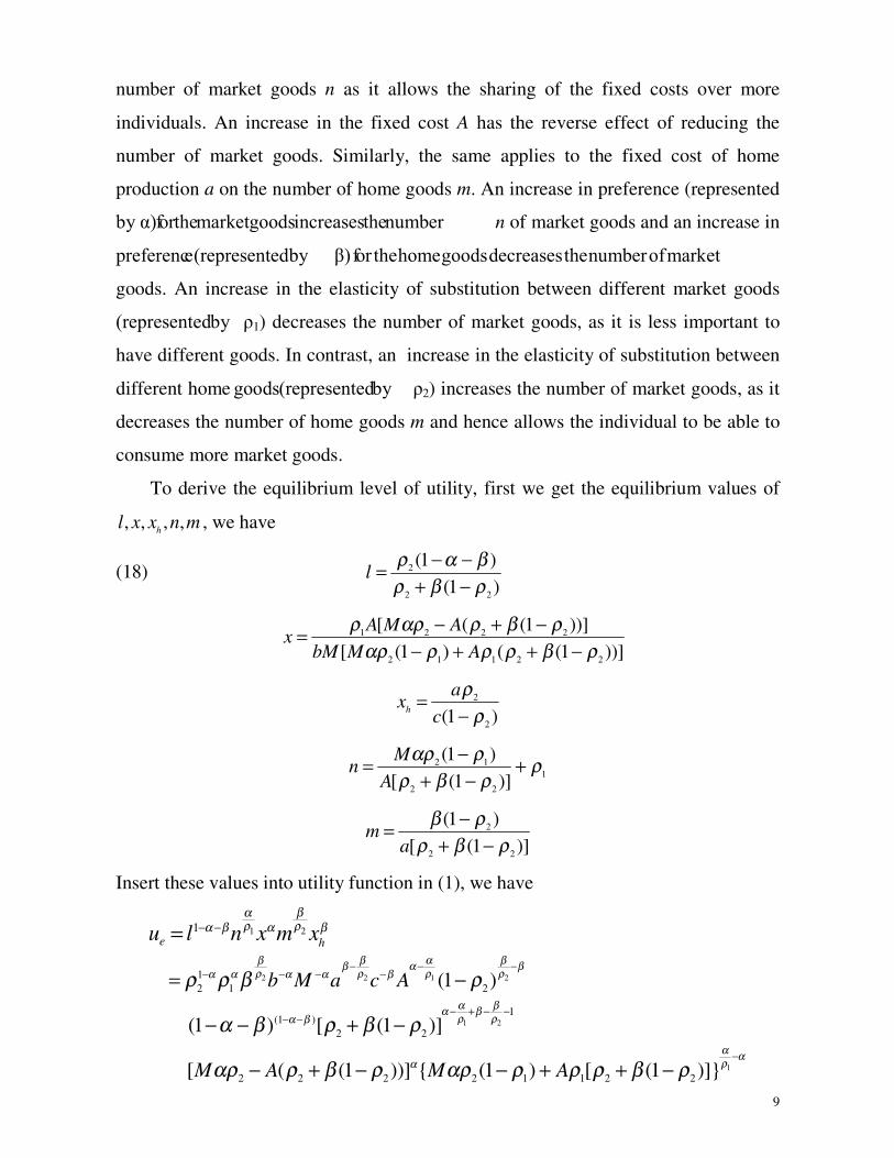
number of market goods n as it allows the sharing of the fixed costs over more
individuals. An increase in the fixed cost A has the reverse effect of reducing the
number of market goods. Similarly, the same applies to the fixed cost of home
production a on the number of home goods m. An increase in preference (represented
E\� .��IRU�WKH�PDUNHW�JRRGV�LQFUHDVHV�WKH�QXPEHU� n of market goods and an increase in
pUHIHUHQFH��UHSUHVHQWHG�E\� ���IRU�WKH�KRPH�JRRGV�GHFUHDVHV�WKH�QXPEHU�RI�PDUNHW�goods. An increase in the elasticity of substitution between different market goods
�UHSUHVHQWHG�E\� !1) decreases the number of market goods, as it is less important to
have different goods. In contrast, an increase in the elasticity of substitution between
different home�JRRGV��UHSUHVHQWHG�E\� !2) increases the number of market goods, as it
decreases the number of home goods m and hence allows the individual to be able to
consume more market goods.
To derive the equilibrium level of utility, first we get the equilibrium values of
, , , ,hl x x n m , we have
(18) 2
2 2
(1 )(1 )
lρ α βρ β ρ
− −=+ −
1 2 2 2
2 1 1 2 2
[ ( (1 ))][ (1 ) ( (1 ))]
A M Ax
bM M Aρ αρ ρ β ρ
αρ ρ ρ ρ β ρ− + −=
− + + −
2
2(1 )h
ax
cρ
ρ=
−
2 11
2 2
(1 )[ (1 )]M
nA
αρ ρ ρρ β ρ
−= ++ −
2
2 2
(1 )[ (1 )]
ma
β ρρ β ρ
−=+ −
Insert these values into utility function in (1), we have
2 2 1 2
1 2
1
1 2
12 1 2
1(1 )
2 2
2 2 2 2 1 1 2 2
1
(1 )
(1 ) [ (1 )]
[ ( (1 ))] { (1 ) [ (1 )]}
e h
b M a c A
M A M A
u l n x m xβ β α ββ α βρ ρ ρ ρα α α α β
α βα βρ ρα β
α αρα
βαρ ρα β βα
ρ ρ β ρ
α β ρ β ρ
αρ ρ β ρ αρ ρ ρ ρ β ρ
− − −− − − −
− + − −− −
−
− −
= −
− − + −
− + − − + + −
=

10
1.3 Optimal output
To analyse the welfare properties, we introduce the government to the model. We let
the government tax home production and subsidize market production. This is not
restrictive as the tax rate and the subsidy rate may either be positive or negative.
Assume that the tax rate of per unit home labor is τ , then consumer’s problem is
(20) Max: u = 1 1 2 21 [ ] [ ]r jr R j J
l x xβα ρ ρρ ρα β− −
∈ ∈∑ ∑ (utility function)
s.t. (1 )r r j jr R j J j J
p x l w l lτ∈ ∈ ∈
+ = − −∑ ∑ ∑ (budget constraint)
jj
l ax
c−
= (production function)
The equilibrium values for above problem are:
(21) 21h
alρ
=−
,
2
2 2
(1 )(1 )
l ρ α βρ β ρ
− −=+ −
,
2
2 2
(1 )( 1)[ (1 )]
ma
β ρτ ρ β ρ
−=+ + −
,
1 11 11 1
2
2 21
[ (1 )] ( )r n
r ss
xp p
ρρ ρ
αρ
ρ β ρ − −
=
=+ − ∑
.
In addition, denoting the subsidy rate per unit of market product as σ , the zero-profit
condition for each firm is
(22) ( )r r rp X b X Aσ= − +
We recalculate the equilibrium values of the various variables to obtain:

11
(23) 1
1
( )( )( 1)
b np
nσ ρ
ρ− −=
−,
1
1
( 1)( ) (1 )
A nX
b nρ
σ ρ−=
− −,
1
1
( 1)( ) (1 )
A nx
b n Mρσ ρ
−=− −
,
2
2
,(1 )h
ax
cρ
ρ=
−
2
2 2
(1 )(1 )
lρ α βρ β ρ
− −=+ −
,
21h
al
ρ=
−,
1
1
( )(1 )r
A nl
nρρ
−=−
,
2 11
2 2
(1 )[ (1 )]M
nA
αρ ρ ρρ β ρ
−= ++ −
,
2
2 2
(1 )( 1)[ (1 )]
ma
β ρτ ρ β ρ
−=+ + −
.
Finally, by requiring a balanced budget for the government, we have
(24) hMm l n Xτ σ=
Using above information, we can get the equilibrium level of utility as
(25)
2 2 2 1 2
1 2
1
2
1 2
12 1 2
1(1 )
2 2
2 2 2 2 1 1 2 2
1
( ) ( 1) (1 )
(1 ) [ (1 )]
[ ( (1 ))] { (1 ) [ (1 )]}
( ) ( 1)
e h
b M a c A
M A M A
B b
u l n x m xβ β β βαβ α βρ ρ ρ ρ ρβα α α α
βαα βρ ρα β
α αρα
βρα
βαρ ρα β βα
ρ ρ β σ τ ρ
α β ρ β ρ
αρ ρ β ρ αρ ρ ρ ρ β ρ
σ τ
− − − −−− − −
− + − −− −
−
−−
− −
= − + −
− − + −
− + − − + + −
= − +
=
where

12
2 1 2
1 2
1
2 (1 )
1
12 1 2
2 2 2 2 2
2 1 1 2 2
(1 ) (1 )
[ (1 )] [ ( (1 ))]
{ (1 ) [ (1 )]}
B M a c A
M A
M A
β βαβ α βρ ρ ρ α β
βαα βρ ρ
α αρ
βρ βα α α
α
ρ ρ β ρ α β
ρ β ρ αρ ρ β ρ
αρ ρ ρ ρ β ρ
− − −− −
− + − −
−
−− −≡ − − −
+ − − + −
− + + −
LV�LQGHSHQGHQW�RI�WKH�WD[�DQG�VXEVLG\�UDWHV� 2�DQG� 1��The effect of a change in tax rate
τ on the equilibrium value of utility with respect to the tax rate, and with the subsidy
rate at whatever level that is allowed by the government budget constraint (24)�DV� 2�varies, evaluated at 0τ = , is given by
(26) 2 1 1 2 2
1 2 2 2 20
[ (1 ) ( (1 )] 0[ ( (1 ))]
e Bb M Adud M A
α
τ
β α ρ ρ ρ ρ β ρτ ρ ρ αρ ρ β ρ
−
=
− + + −= >− + −
This means that, starting from the original position without any tax/subsidy, a tax on
home production which finances for a subsidy on market production increases utility,
ignoring administrative costs and any possible side effects, such as rent-seeking
activities triggered by the subsidy. Since all firms just break-even in equilibrium, we
may base our welfare comparisons simply on the utility levels alone. We thus have,
Proposition 1: In our model with both home and market production under the
conditions of increasing returns and average-cost pricing, a subsidy, if not
excessive, on market production financed by a tax on home production improves
efficiency even if the initial position involves no tax distortion, ignoring
administrative costs and any possible side effects.
The possibility for efficiency improvements through some tax/subsidy means
that the original equilibrium is not perfectly efficient. What is the source of this
imperfect efficiency? We view the imperfect efficiency as a result of the combination
of increasing returns and average-cost pricing in market goods. In the model, there
are also increasing returns in home production. However, since the
individual/household concerned makes the decision to produce/consume, the
implications of increasing returns are taken into account and hence the optimizing
choice does not result in any inefficiency. On the other hand, market goods produced

13
by firms are sold to individuals at average costs. Since each consumer take the price
of each of this good as given, the demand functions for these market goods do not
take the implications of increasing returns into account. Each consumer assumes that,
no matter how much she buys, the price will not be affected. However, if all
consumers buy more of a market good, the fixed cost component of producing this
good will be spread over a larger number of units, result in a lower average cost and
hence lower price for every consumer. This effect is not taken into account and hence
we have the under-production of the market goods. Subsidizing market goods
financed by taxing home production may thus be utility increasing. Put it differently,
the fixed cost component of a market good may be viewed as possessing a publicness
characteristic since it is shared by all consumers. The under-consumption/production
of market goods may be said to be related to the public-good nature of the fixed-cost
components.
The taxing of home production may not be practically feasible and a lump-sum
tax or poll tax may not be politically feasible or distributionally desirable. The
subsidy on market production may thus be impracticable. However, if we allow for
different degrees of increasing returns between different market goods, it may be
feasible to tax market goods with lower degrees of increasing returns and subsidize
market goods with higher degrees of increasing returns, as the next section shows.
2. A model with home and differentiated market production
In this section, the model of the previous section is extended to allow for different
sectors of market goods that may have different degrees of elasticity of substitution
and different degrees of increasing returns (through different values of the fixed cost
and marginal cost). Instead of (1), we now have
(1’) Max: u = 1 2
1 2 1 1 2 2
1 2
1 [ ] [ ] [ ]r jkr R j Jk R
l x x xα α βρ ρ ρα α β ρ ρ ρ− − −
∈ ∈∈∑ ∑ ∑ (utility function)
s.t. 1 2
(1 )r r jk kr R j Jk R
p x p x w l l∈ ∈∈
+ = − −∑ ∑ ∑ (budget constraint)
14
jj
l ax
c−
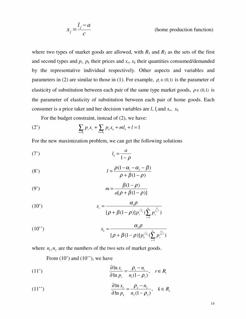
= (home production function)
where two types of market goods are allowed, with R1 and R2 as the sets of the first
and second types and pr, pk their prices and xr, xk their quantities consumed/demanded
by the representative individual respectively. Other aspects and variables and
parameters in (2) are similar to those in (1). For example, (0,1)iρ ∈ is the parameter of
elasticity of substitution between each pair of the same type market goods, (0,1)ρ ∈ is
the parameter of elasticity of substitution between each pair of home goods. Each
consumer is a price taker and her decision variables are l, lj and xr, xk
For the budget constraint, instead of (2), we have:
(2’) 1 2
1r r k k hr R k R
p x p x ml l∈ ∈
+ + + =∑ ∑
For the new maximization problem, we can get the following solutions
(7’) 1h
al
ρ=
−
(8’) 1 2(1 )(1 )
lρ α α β
ρ β ρ− − −=+ −
(9’) (1 )
[ (1 )]m
aβ ρ
ρ β ρ−=
+ −
(10’) 1 11
1 11 1
1
1
[ (1 )] ( )nr
r ss
xp p
ρρ ρ
α ρ
ρ β ρ − −
=
=+ − ∑
(10’’) 21 2
1 12 2
2
1
[ (1 )] ( )nk
k ss
xp p
ρρ ρ
α ρ
ρ β ρ − −
=
=+ − ∑
where 1 2,n n are the numbers of the two sets of market goods.
From (10’) and (10’’), we have
(11’) 1 11
1 1
ln,
ln (1 )r
r
x nr R
p nρ
ρ∂ −= ∈∂ −
(11’’) 2 22
2 2
ln,
ln (1 )k
k
x nk R
p nρ
ρ∂ −= ∈∂ −

15
Let the production functions of market goods be
1 1 1( ) / ,r rX l A b r R= − ∈
2 2 2( ) / ,k kX l A b k R= − ∈
so that the labor cost functions of market goods are
(12’) 1 1 1,r rl b X A r R= + ∈
(12’’) 2 2 2,k kl b X A k R= + ∈
The zero profit condition gives
(15’ ) 1 1 1,r r rp X b X A r R= + ∈
(15’’ ) 2 2 2,k k kp X b X A k R= + ∈
Similarly to the derivation of (16), we may derive
(16’) 1 1 11
1 1
( )( 1)
b np
nρ
ρ−=−
,
2 2 22
2 2
( )( 1)
b np
nρ
ρ−=−
,
1 1 11
1 1 1
( 1)(1 )
A nX
b nρ
ρ−=
−,
2 2 22
2 2 2
( 1)(1 )
A nX
b nρ
ρ−=
−,
1 1 11
1 1 1
( 1)(1 )A n
xb n Mρ
ρ−=
−,
2 2 22
2 2 2
( 1)(1 )A n
xb n Mρ
ρ−=
−,
1 2(1 )(1 )
lρ α α β
ρ β ρ− − −=+ −
,
1h
al
ρ=
−,
(1 )h
ax
cρ
ρ=
−
1 1 11
1 1
( )(1 )
A nl
nρ
ρ−=
−,

16
2 2 22
2 2
( )(1 )
A nl
nρ
ρ−=
−,
1 11 1
1
(1 )[ (1 )]M
nA
α ρ ρ ρρ β ρ
−= ++ −
,
2 22 2
2
(1 )[ (1 )]
Mn
Aα ρ ρ ρρ β ρ
−= ++ −
,
(1 )[ (1 )]
ma
β ρρ β ρ
−=+ −
.
Their comparative statics are:
(17’) 1 1 1(1 )0,
[ (1 )]nM A
α ρ ρρ β ρ
∂ −= >∂ + −
1 1 12
1 1
(1 )0,
[ (1 )]n MA A
α ρ ρρ β ρ
∂ −= − <∂ + −
1 1
1
(1 )0,
[ (1 )]n M
Aρ ρ
α ρ β ρ∂ −= >∂ + −
1 1 12
1
(1 )(1 )0,
[ (1 )]n M
Aα ρ ρ ρ
β ρ β ρ∂ − −= − <∂ + −
1 1
1 1
1 0[ (1 )]
n MA
α ρρ ρ β ρ
∂ = − + <∂ + −
1 1 12
1
(1 )0
[ (1 )]n M
Aα β ρ
ρ ρ β ρ∂ −= >∂ + −
Similarly, 2 0nM
∂ >∂
, 2
2
0nA
∂ <∂
, 2
2
0nα
∂ >∂
, 2
2
0nρ
∂ <∂
, 2nρ
∂∂
> 0
2
(1 )0,
[ (1 )]m
aρ ρ
β ρ β ρ∂ −= >∂ + −
2
(1 )0,
[ (1 )]ma a
β ρρ β ρ
∂ −= − <∂ + −
20
[ (1 )]m
aβ
ρ ρ β ρ∂ −= <∂ + −
.
The qualitative results of the comparative statics are again consistent with intuition.

17
To analyse the welfare properties, we introduce the government to the model
and allow the government to tax or subsidize market production but not home
production. Denote the tax/subsidiy rate of per unit of each market good in set one as
1τ (positive if tax; negative if subsidy) and that on set two as 2τ . Then, the zero profit
conditions for firms are
(22’) 1 1 1 1( ) ,r r rp X b X A r Rτ= + + ∈
(22’’) 2 2 2 2( ) ,k k kp X b X A k Rτ= + + ∈
The equilibrium values of the various variables are given by:
(23’) 1 1 1 11
1 1
( )( )( 1)
b npn
τ ρρ+ −=
−,
2 2 2 22
2 2
( )( )( 1)
b npn
τ ρρ+ −=
−,
1 1 11
1 1 1 1
( 1)( ) (1 )
A nXb n
ρτ ρ
−=+ −
,
2 2 22
2 2 2 2
( 1)( ) (1 )
A nXb n
ρτ ρ
−=+ −
,
1 1 11
1 1 1 1
( 1)( ) (1 )
A nxb n M
ρτ ρ
−=+ −
,
2 2 22
2 2 2 2
( 1)( ) (1 )
A nxb n M
ρτ ρ
−=+ −
,
1 2(1 )(1 )
l ρ α α βρ β ρ− − −=+ −
,
1hal
ρ=
−,
(1 )hax
cρ
ρ=
−
1 1 11
1 1
( )(1 )
A nln
ρρ
−=−
,
2 2 22
2 2
( )(1 )
A nln
ρρ
−=−
,

18
1 11 1
1
(1 )[ (1 )]
MnA
α ρ ρ ρρ β ρ
−= ++ −
,
2 22 2
2
(1 )[ (1 )]
MnA
α ρ ρ ρρ β ρ
−= ++ −
,
(1 )[ (1 )]
ma
β ρρ β ρ
−=+ −
.
The balanced budget requirement for the government gives
(24’) 1 1 1 2 2 2 0n X n Xτ τ+ =
The equilibrium utility value is given by
(25’)
1
1 2 1
2
1 2
11 2 1 11
1
1 1 1 1 2 22
1 1 1 1 2
2 2 2
1 21 2 1 1 2 21
1 1 2 2
(1 ) (1 )( ) { }(1 ) [ (1 )]
[ ( (1 ))] (1 ){ } { }[ (1 ) ( (1 ))] [ (1 )]
[{
e h
MA
A M A MM M A A
A M A
u l n x n x m xα
α α β ρ
αα ρ
α α βα α β ρ α ρ α ρ β
ρ α α β α ρ ρ ρρ β ρ ρ β ρ
ρ α ρ ρ β ρ α ρ ρ ρα ρ ρ ρ ρ β ρ ρ β ρ
ρ α ρ
− − −
− − −
− − − −= ++ − + −
− + − − +− + + − + −
−
=
2
1 2
2
2 2 2 2
1 1 2 2
1 21 1 2 2
( (1 ))] }[ (1 ) ( (1 ))]
(1 ){ } [ ] ( ) ( )[ (1 )] (1 )
( ) ( )
M M A
a b ba c
B b b
α
βα αρ β
α α
ρ β ρα ρ ρ ρ ρ β ρ
β ρ ρ τ τρ β ρ ρ
τ τ
− −
− −
+ −− + + −
− + ++ − −
= + +
where
1
1 2 1
2
1 2
11 2 1 11
1
1 1 1 1 2 22
1 1 1 1 2
2 2 2 2
2 2 2 2
(1 ) (1 )( ) { }(1 ) [ (1 )]
[ ( (1 ))] (1 ){ } { }[ (1 ) ( (1 ))] [ (1 )]
[ ( (1 ))]{[ (1 ) ( (1 )
MBA
A M A MM M A A
A M AM M A
αα α β ρ
αα ρ
ρ α α β α ρ ρ ρρ β ρ ρ β ρ
ρ α ρ ρ β ρ α ρ ρ ρα ρ ρ ρ ρ β ρ ρ β ρ
ρ α ρ ρ β ρα ρ ρ ρ ρ β ρ
− − −− − − −≡ ++ − + −
− + − − +− + + − + −
− + −− + + −
2(1 )} { } [ ]
)] [ (1 )] (1 )a
a c
βα ρ ββ ρ ρ
ρ β ρ ρ−
+ − −
is independent of the tax/subsidy rates. We calculate the derivative of equilibrium
utility level with respect to the tax rate 1τ , with the value of 2τ given by the
government budget constraint (24’) as 1τ varies, evaluated at 1 0τ = , 2 0τ = , yielding

19
(26’)
1 2
1
1 2 1 1 2 1 2 21
1 1 2 2 2 20
{ [ { [
{ [
{ (1 )]} (1 )]}(1 )]}
e B M A M Adud b b M Aα α
τ
ρ α α ρ ρ β ρ ρ α α ρ ρ β ρτ ρ α ρ ρ β ρ+
=
− + − − − + −=− + −
From (26’), it can be seen that
(27)
11 0
/ 0edud
ττ
=
> <
if 1 1 1 2 2 2
1 2
[ ( (1 ))] [ ( (1 ))]/M A M Aρ α ρ ρ β ρ ρ α ρ ρ β ρα α
− + − − + −> <
To see the meaning of this condition, consider the following three simple cases:
1. The case of�!1 � !2�DQG� .1 � .2 when the condition collapses into -A1 > -A2, or
A1 < A2. This means that, ceteris paribus, if the fixed cost component in the
production of market goods of sector one is smaller than that of sector two, it
is efficient to tax sector one and subsidize sector two.
2. 7KH�FDVH�RI� .1 � .2 and A1 = A2�ZKHQ�WKH�FRQGLWLRQ�FROODSVHV�LQWR� !1 !� !2. This
means that, ceteris paribus, if the elasticity of substitution between goods
within sector one is larger than that within sector two, it is efficient to tax
sector one and subsidize sector two.
3. TKH�FDVH�RI� !1 � !2 and A1 = A2�ZKHQ�WKH�FRQGLWLRQ�FROODSVHV�LQWR� .1 !� .2. This
means that, ceteris paribus, if the preference of individuals is such that goods
in sector one is regarded as more important than those in sector two, it is
efficient to tax sector one and subsidize sector two.
The intuitive reasons for the three separate points above may be briefly explained.
The first point relates to the degree of increasing returns; the higher the fixed cost, the
higher the degree of increasing returns and the larger is the publicness characteristic.
The elasticity of substitution between goods (second point) is also relevant. The more
substitutable are goods within a sector, ceteris paribus, the less number of goods of
that sector will be produced and more of each good will be produced. (This point is
confirmed below.) Then, given that the fixed cost is the same, the degree of
increasing returns is lower at higher output. (Defining the degree of increasing returns

20
as the negative of the elasticity of average cost with respect to output, this point may
be verified simply by differentiation.) Thus, the sector with a higher elasticity of
substitution between goods within that sector has lower degree of increasing returns.
A tax on the sector with higher elasticity of substitution and a subsidy on the sector
with lower elasticity of substitution is thus taxing the sector with lower degree of
increasing returns and subsidising the sector with a higher degree of increasing
returns.
The point that, ceteris paribus, higher elasticity of substitution leads to a lower
number of goods and higher output for each good may be verified. The effect on the
number of goods is given by i
i
nρ
∂∂
being negative in (17’). The effect on output can be
obtained by first substitute the solution for, say, n1 into that for X1 from (23’),
obtaining
1 1 1 11
1 1 1 1 1
{ [{ [
(1 )]}(1 ) (1 )]}
A M AXb M A
ρ α ρ ρ β ρα ρ ρ ρ ρ β ρ
− + −=− + + −
Partial differentiation gives
11 1 1 1
1
{ [ (1 )]} 0X b M M Aα ρ α ρ ρ β ρρ
∂ = − + − >∂
where the positivity follows from the numerator in the expression for X1 above.
We may now consider the third point above on the effect of the degree of
preference. The more important is a sector regarded by individuaOV��WKH�KLJKHU�LV� .i),
the more of the goods in that sector are consumed. This again results in a higher
output level for goods in that sector, i.e. a higher Xi. This again leads to a lower
degree of increasing returns. Thus, ceteris paribus, a tax on this sector and a subsidy
on a sector with lower importance will be efficient. (This is in line with the result of
Heal 1980 that large markets are over-served and small markets are under-served.)
Thus, all the three elements of fixed cost, elasticity of substitution, and preference
importance parameter are relevant and they all relates to the degree of increasing
returns. When more than one of these three elements differ, their effects intertwine
and the net effects are as given in (27). Our results may be summarized as

21
Proposition 2: In our model with both home and market production under the
conditions of increasing returns and average-cost pricing with two sectors of
different fixed costs, elasticities of substitution, and degree of importance in
preference, it is efficient to tax the sector with lower fixed costs, higher elasticity
of substitution and/or higher degree of importance in preference and subsidize
the other in accordance to (27).
3. Concluding Remarks
Despite the straightforward nature of our results as summarized in the two
propositions, the applicability to the real economy is subject to important
qualifications. First, the government may not have the information to differentiate
which goods should be taxed (and by how much) and which subsidized. Allowing
differential tax/subsidies may open a flood gate of rent-seeking activities causing
more waste than the efficient gain that could be obtained. Secondly, we have not
considered other factors causing imperfect efficiency in the real economy. One
important factor is environmental disruption of many production and consumption
activities. If the degrees of such disruption are not related to whether a good is home
produced or produced for the market, our conclusions may not be much affected.
However, there may be some presumption that home production activities are
generally less environmentally disruptive than market production. Most of home
production consists of home cooking, cleaning, washing, gardening, and childcare,
which are largely non-disruptive except for the detergents used. Thus, on the
environmental issue, market production should be taxed instead. However, this
consideration is to a large extent at least offset by the pre-existence of general
taxation including income taxes and value-added or goods and services taxes. These
taxes do not fall on home production (the intermediate goods used in home
production are produced for the market). If we view these general taxes as largely
offsetting to the higher degrees of environmental disruption of most market goods,
then the differential degrees of disruption between home and market goods no longer
affect our conclusion on the efficiency of subsidizing market goods with higher

22
degrees of increasing returns. The desirability of doing so is then mainly qualified by
the first consideration on the lack of information and the promotion of rent-seeking
activities.
References
ADES, Alberto F. & Glaeser, Edward L. (1999), ‘Evidence on growth, increasing
returns, and the extent of the market’, Quarterly Journal of Economics,
114(3):1025-45.
ANTWEILER, Werner & TREFLER, Daniel (2002), ‘Increasing returns and all that:
A view from trade’, American Economic Review, 92: 93-119.
ARROW, Kenneth J. (1995), ‘Returns to scale, information and economic growth’, in
Koo & Perkins.
ARROW, Kenneth J., NG, Yew-Kwang & YANG, Xiaokai, eds. (1998), Increasing
Returns and Economic Analysis, London: Macmillan.
ARTHUR, W.B. (1994), Increasing Returns and Path Dependence in the Economy,.
Ann Arbor: University of Michigan Press.
BUCHANAN, James M. & YOON, Y.J., (eds.) (1994a), The Returns to Increasing
Returns. Ann Arbor: University of Michigan Press.
BUCHANAN, James M. & YOON, Yong J. (1994b), Increasing returns, parametric
work-supply adjustment, and the work ethic. In Buchanan & Yoon (1994a), pp.
343-356.
DIXIT, Avinash K. & STIGLITZ, Joseph E. (1977), ‘Monopolistic competition and
optimum product diversity’, American Economic Review, 67 (3): 297-308.
ETHIER, Wilfred (1979), ‘Internationally decreasing costs and world trade’, Journal
of International Economics, 9: 1-24.
HEAL, Geoffrey (1980), ‘Spatial structure in the retail trade: a study in product
differentiation with increasing returns’, Bell Journal of Economics, 11(2):545-83.
HEAL, Geoffrey (1999), The Economics of Increasing Returns, Edward Elgar.

23
KOO, Bon H. & PERKINS, Dwight H. (1995), Social Capability and Long-Term
Economic Growth, London: Macmillan.
LANCASTER, Kelvin (1990), The economics of product variety, Management
Science, 9(3): 189-206.
Locay, L. (1990), Economic development and the division of production between
households and markets, Journal of Political Economy, 98: 965-82.
RADNER, Roy & STIGLITZ, Joseph (1984), ‘A non-concavity in the value of
information’, Ch. 3 of Boyer & Kihlstrom.
ROMER, P. (1986), ‘Increasing returns and long-run growth’, Journal of Political
Economy, 94:1002-37.
YANG, Xiaokai & Heijdra, B. (1993), “Monopolistic Competition and Optimum
Product Diversity: Comment”, American Economic Review, 83: 295-301.
YANG, Xiaokai & NG, Yew-Kwang (1993), Specialization and Economic
Organization: A New Classical Microeconomic Framework, Amsterdam: North-
Holland.
YANG, Xiaokai & SHI, Heling (1992), "Specialization and Product Diversity",
American Economic Review, 82: 392-398.
WILSON, Robert (1975), ‘Informational economies of scale’, Bell Journal of
Economics and Management Science, 184-195.