Availability Bias & Sensitivity AnalysisProblems with bad data

Models and Specification

We let an equation (aka model) stand for the data

If the model is a good representation of the data, then our inferences are likely to be good.

A model is said to be misspecified if the terms in the equation do not correspond correctly to the phenomenon we are representing

In meta-analysis, there may be many unknown moderators that are missing from the equation, or there may be moderators included in the model that should be absent. Finding an adequate model is important.

Availability Problem

Missing at random is okay for inference if the model is properly specified

Nonrandom is a problem

Sources of nonrandom samples of studiesPublication bias – significant, small N

Language bias (English; more stat sig)

Availability to the researcher (friends help)

Familiarity-stuff in one’s own field

Duplication- significant study appears more than once in the lit

Citation – significant studies more likely cited

Dissertations; other filedrawer hard to find

Deliberate misrepresentation for financial reasons

Bias QuestionsEvidence of any bias?

Does Bias nullify the effect?

If not, what is the impact and best estimate of the effect?

How would we know?Registries of studies yet to be conductedFrom observed data themselvesIt’s hard to be conclusive about bias unless someone admits fraud

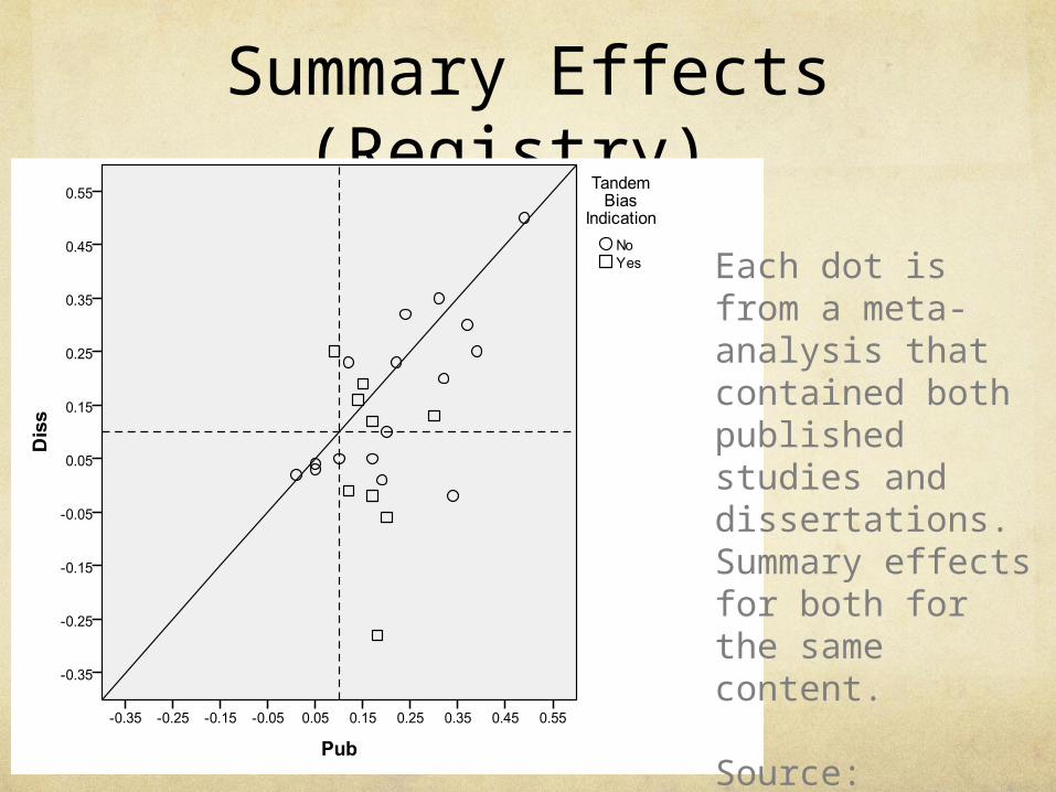
Summary Effects (Registry)

Each dot is from a meta-analysis that contained both published studies and dissertations. Summary effects for both for the same content.

Source: Ferguson & Brannick, 2012, Psych Methods

Forest PlotDrift to the right by precision? Effects of second hand smoke on cancer incidence.

Source: Borenstein, Hedges, Higgins & Rothstein, 2009, p. 282

Precision Forest Plot in R

Sort your effect sizes by Vi or SEi before (or after) importing to R. Them run the forest plot.install.packages("metafor")library(metafor)install.packages("xlsx")library(xlsx)dataRocks <- read.xlsx("/Users/michaelbrannick/Desktop/RocksLMX_AC2.xlsx",sheetName="Sheet1”)

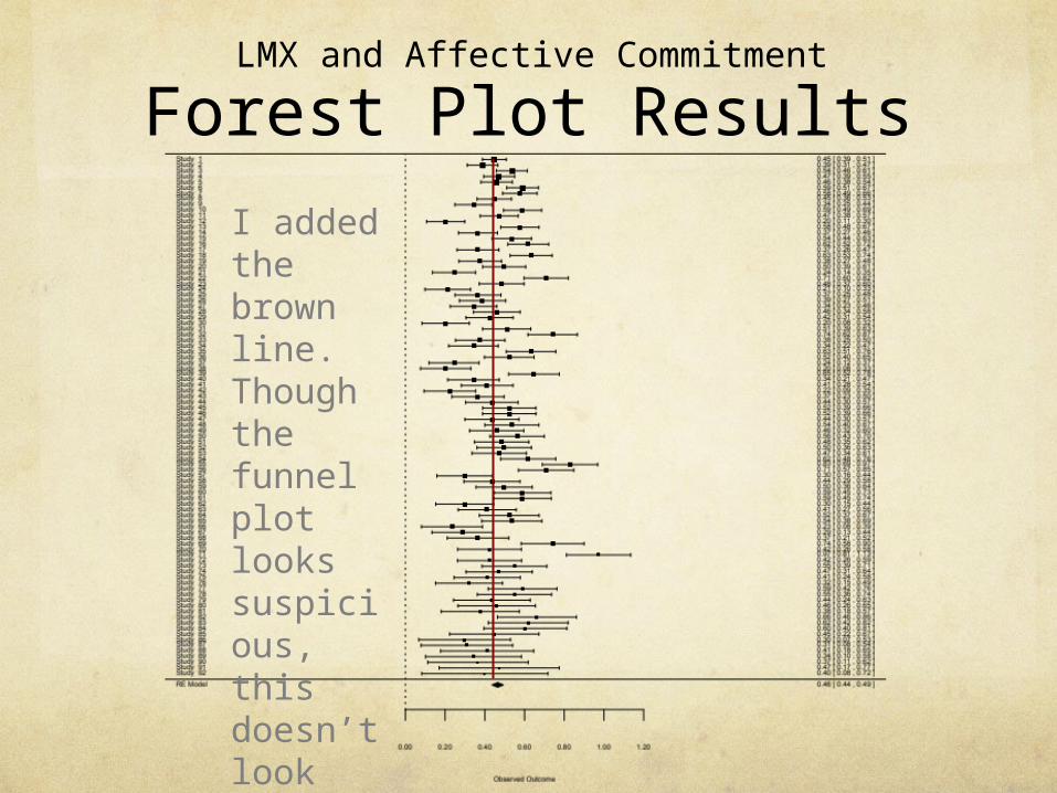
Forest Plot Results

I added the brown line. Though the funnel plot looks suspicious, this doesn’t look bad to me.

LMX and Affective Commitment

Trim & FillCreates symmetry;Adjusts summary ES

Source: Borenstein, Hedges, Higgins & Rothstein, 2009, p. 287

Trim-and-fill is a kind of sensitivity analysis. Do not consider the results of the symmetrical (augmented) data as more valid than the original. More a ‘what if’ analysis.

Trim-and-fill in R

Ordinary funnel

Trim-and-Fill Results

Note the syntax required to get the plot. Print the results (e.g., resRocks2) to see the adjusted mean.

Oddly enough, the program inferred that there were too many studies on the low side, not the high side. Therefore, the best estimate is probably the original, unadjusted one.

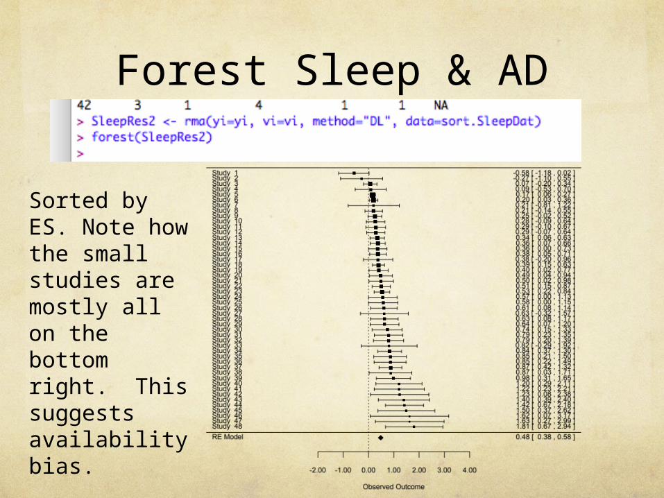
Forest Sleep & AD

Sorted by ES. Note how the small studies are mostly all on the bottom right. This suggests availability bias.

Trim & Fill Sleep n AD

This is one of the worst cases of APPARENT publication bias (funnel asymmetry) that I’ve seen.

Exercise

Upload the dataset TnFEx.xlsx

Compute a trim-and-fill analysis for the overall effect size.

What is the overall ES before and after?

What is your conclusion about publication bias and its implication for the overall effect size?

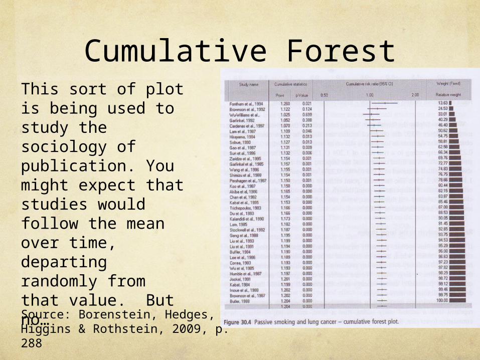
Cumulative Forest

Source: Borenstein, Hedges, Higgins & Rothstein, 2009, p. 288

This sort of plot is being used to study the sociology of publication. You might expect that studies would follow the mean over time, departing randomly from that value. But no…

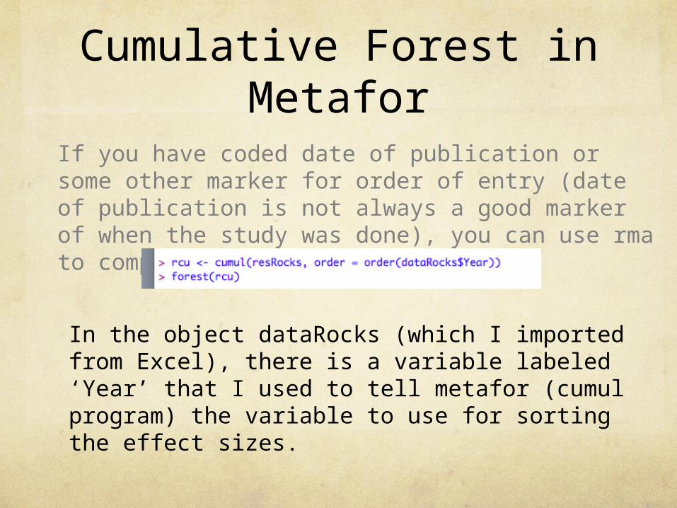
Cumulative Forest in Metafor

If you have coded date of publication or some other marker for order of entry (date of publication is not always a good marker of when the study was done), you can use rma to compute this.

In the object dataRocks (which I imported from Excel), there is a variable labeled ‘Year’ that I used to tell metafor (cumul program) the variable to use for sorting the effect sizes.

I added the brown line. It is clear from the analysis that the significance (rho = 0) was never an issue. This kind of analysis is common in medicine, where there are often very small effect sizes.

There are some jumps in the progression. Notice how the confidence interval expands when there is a jump early on. This is because the discrepant study increases the REVC while decreasing the sampling variance. This is a random (varying) effects analysis.

Cumulative Forest for LMX – AC Data

Egger’s RegressionTi = effect size; vi=sampling variance of ES

iii vTz /

iii vz )/1(10

Should be flat (centered) if no bias (beta1 is zero). This shows small studies have higher values. Significant negative slope (beta1) is concerning.

Source: Sutton (2009). In Cooper, Hedges, & Valentine (Eds) Handbook fo Research Synthesis Methods p. 441

Funnel Asymmetry Test

Metafor offers several different tests for funnel plot asymmetry (variations on Egger’s test; see Viechtbaur 2010 for a list of references). The default test is shown below for the LMX data.

The slope appears quite flat, and we have about 90 ES, so there is some power for the test. Thus funnel plot asymmetry indicative of publication bias does not appear likely in this example.

Radial PlotCrude approximate explanation: This plot shows how the effect size (y-axis) relates to the weight (x-axis). Line is drawn from zero on y-axis. Not a typical regression. Forced zero intercept. Assumed no effect of treatment.

LMX – Affective Commitment Data

>radial(resRocks)

More technically accurate, but harder to remember: the plot shows the standardized ES as a function of the precision (square root of the weight).

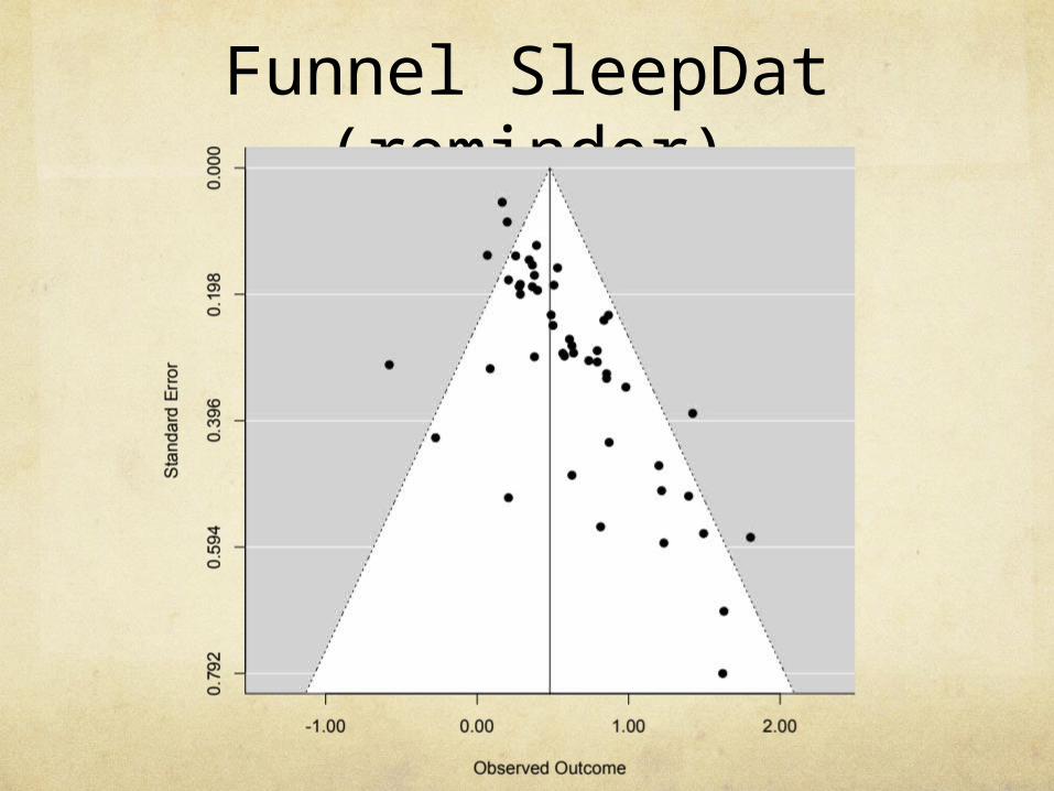
Funnel SleepDat (reminder)

Radial (SleepRes)

Precision Forest (SleepDat)

Exercise – Funnel Test

Recall the TnF dataset

Run a test of funnel asymmetry on these data (use the standard RE meta-analysis model).

What is your result?

What is your interpretation of the finding?

Problems with Diagnostics

Small study effectsSmall studies may actually have larger effects (not bias).

What characteristics are associated with larger vs. smaller N studies?

HeterogeneityFunnel, trim-and-fill designed for common-effects model

Really should be residuals after removing moderators

What Else Can We Do?

Maybe there is bias in the sample

Maybe there is bad data

Does it matter?

Sensitivity Analysis

Outliers. Run twice. Share both results with your reader.

Source: Greenhouse & Iyengar (2009). In Cooper, Hedges, & Valentine (Eds) Handbook fo Research Synthesis Methods p. 422

Finding Outliers (1)

Externally standardized residuals are compared to a distribution of residuals from a model in which that observation is excluded. Metafor uses rstudent() to find these. Most meaningful in the context of meta-regression (moderator analysis).

Finding Outliers (2)

This is the result of an analysis with no moderators – it is the overall result for the varying (random) effects analysis. Equivalent to a regression with intercept only.

Finding Outliers (3)This analysis considers the study sample size and the REVC in addition to the raw distance to the mean. Look for ‘large’ values – the z refers to the unit normal, so |2| is large, but I would probably start with 2.5 or 3. Your call though. I would export and sort with Excel (there are 92 residuals in this analysis).

LMX data

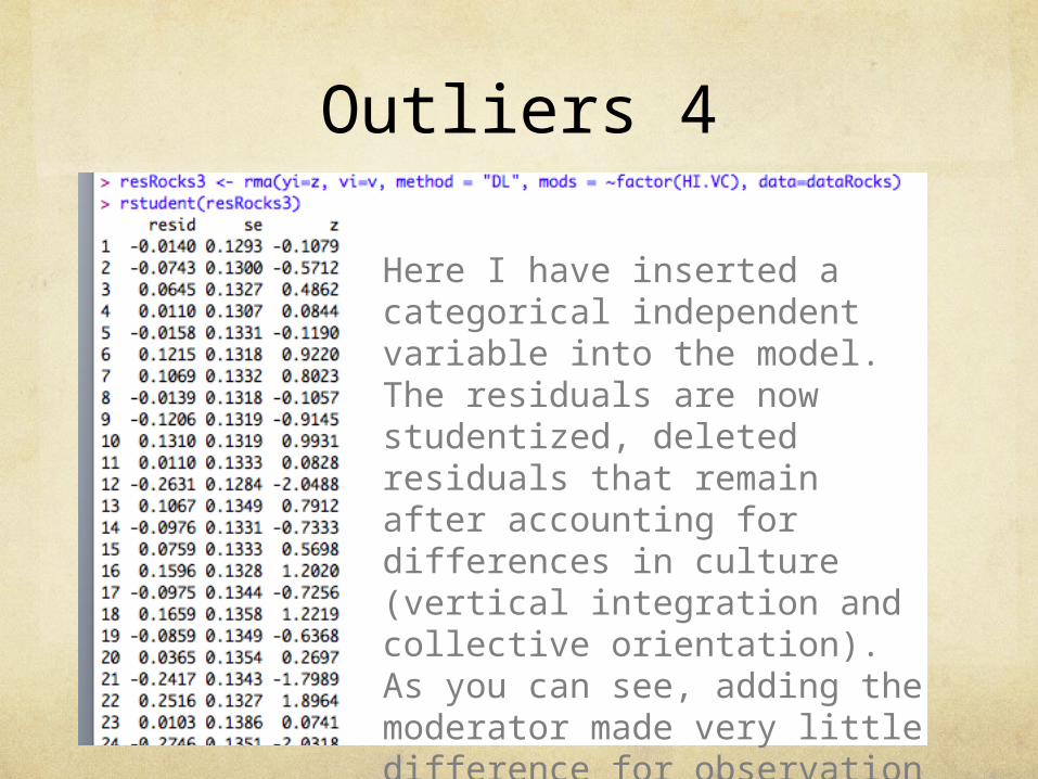
Outliers 4

Here I have inserted a categorical independent variable into the model. The residuals are now studentized, deleted residuals that remain after accounting for differences in culture (vertical integration and collective orientation). As you can see, adding the moderator made very little difference for observation 12 (-2.08 to -2.05). For an important moderator, there could be a large difference.

If you show that the impact of outliers and nuisance variables (and moderators) is minimal or at least not a threat to your inferences, then your conclusions will be more credible.

Leave One Out

In this sensitivity analysis, every study is removed, 1 by 1, and the overall ES is re-estimated.

Helpful to judge the impact of influential studies (sometimes outlying ES, sometimes very large N)

Can be run in rma if the model has no moderators (i.e., for overall ES or a subset of studies)

Two uses for thisFind and remove problematic studies

Share summary of findings with your reader

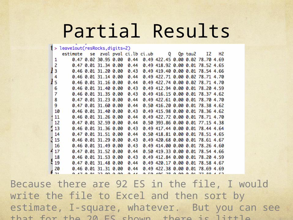
Partial Results

Because there are 92 ES in the file, I would write the file to Excel and then sort by estimate, I-square, whatever. But you can see that for the 20 ES shown, there is little impact from dropping each study.

Exercise

Using the Devine data, runOutlier analysis (with publication vs. dissertation included in the model)

Leave-one-out analysis (without the moderator)

Delete any problematic studies (can use Excel)

Rerun the analysis without problematic studies

What is your new result?

Does your conclusion or inference change?

Fail-safe N

How many studies do we need to make the result n.s.? (Rosenthal) [this is an older analysis – I don’t recommend it.]

How many studies do we need to make the summary effect small enough to ignore? (Orwin)

fsc

cobtobtfs dd

ddkk

)( kfs = failsafe studies

kobt = studies in metadobt = summary ESdc = desired lower boutnddfs= studies with this (eg 0 or less) size needed to lower ES

Corwin, R. G. (1983). A fail-safe N for effect size in meta-analysis. Journal of Educational Statistics, 8, 157-159.

Favors Ground

FavorsOnline

Meta-analysis of 71Samples (studies) comparing classroom instruction versus online instruction on tests of declarative knowledge (college classes and corporate training).

Red line at bottom shows expected outcomes. Average difference near zero, but SUBSTANTIAL variability. Begs us to ask why the study outcomes are so different.

Red is random effects.Orange is fixed effects.

Add moderators.

Individual Studies

Previous methods all concern the mean of studies or overall effect size.

What if we are interested in the effect size for an individual study?

If common effects, the effect size for all studies is the mean, so we have nothing to estimate.

If varying effects, there is uncertainty about the true location of the study’s effect size. Bayesian thinking moves individual studies toward the mean. Can also get a confidence interval for the revised estimate.

Sensitivity Analysis -TauVarying levels of tau-squared

This graph shows the effect of the magnitude of tau-squared on the posterior estimates. As tau-squared increases, the effects spread out and there are some ordinal changes, too.